Simplifying ML: Impact of degree of polynomial degree on bias & variance and other insights

This post takes off from my earlier post Simplifying Machine Learning: Bias, variance, regularization and odd facts- Part 4. As discussed earlier a poor hypothesis function could either underfit or overfit the data. If the number of features selected were small of the order of 1 or 2 features, then we could plot the data and try to determine how the hypothesis function fits the data. We could also see whether the function is capable of predicting output target values for new data.

However if the number of features were large for e.g. of the order of 10’s of features then there needs to be method by which one can determine if the learned hypotheses is a ‘just right’ fit for all the data.

Checkout my book ‘Deep Learning from first principles Second Edition- In vectorized Python, R and Octave’. My book is available on Amazon as paperback ($18.99) and in kindle version($9.99/Rs449).

You may also like my companion book “Practical Machine Learning with R and Python:Second Edition- Machine Learning in stereo” available in Amazon in paperback($12.99) and Kindle($9.99/Rs449) versions.

The following technique can be used to determine the ‘goodness’ of a hypothesis or how well the hypothesis can fit the data and can also generalize to new examples not in the training set.

Several insights on how to evaluate a hypothesis is given below

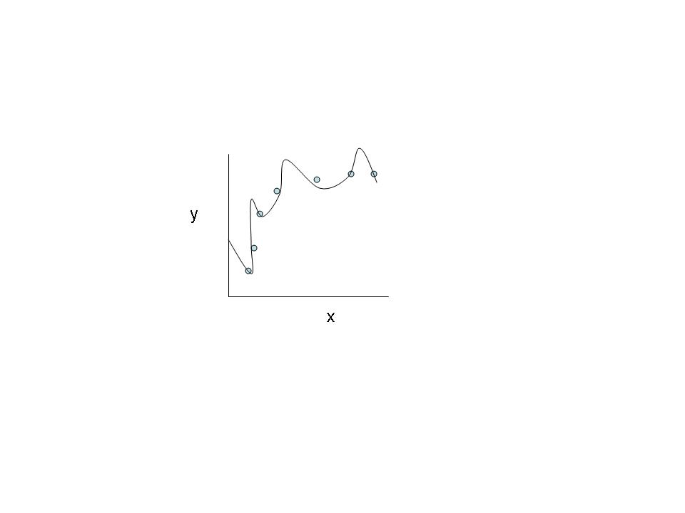
Consider a hypothesis function

h_Ɵ (x) = Ɵ₀ + Ɵ₁x₁ + Ɵ₂x₂² + Ɵ₃x₃³ + Ɵ₄x₄⁴

The above hypothesis does not generalize well enough for new examples in the data set.

Let us assume that there 100 training examples or data sets. Instead of using the entire set of 100 examples to learn the hypothesis function, the data set is divided into training set and test set in a 70%:30% ratio respectively

The hypothesis is learned from the training set. The learned hypothesis is then checked against the 30% test set data to determine whether the hypothesis is able to generalize on the test set also.

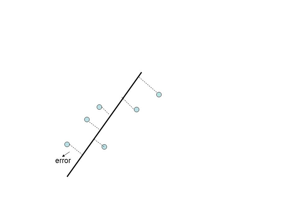
This is done by determining the error when the hypothesis is used against the test set.

For linear regression the error is computed by determining the average mean square error of the output value against the actual value as follows

The test set error is computed as follows

J_test(Ɵ) = 1/2m_testΣ(hƟ (x_testⁱ – y_testⁱ)²

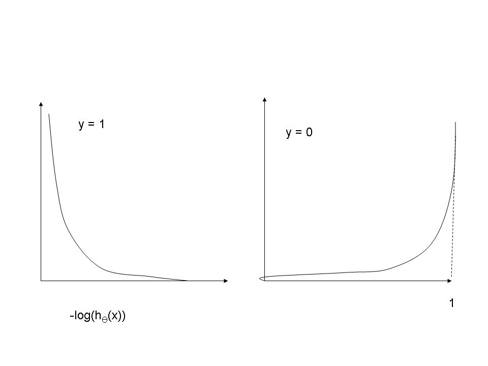
For logistic regression the test set error is similarly determined as

J_test(Ɵ) = = 1/m_test Σ -y_test * log(h_Ɵ(x_test)) – (1-y_test) * (log(1 – h_Ɵ(x_test))

The idea is that the test set error should as low as possible.

Model selection

A typical problem in determining the hypothesis is to choose the degree of the polynomial or to choose an appropriate model for the hypothesis

The method that can be followed is to choose 10 polynomial models

h_Ɵ (x) = Ɵ₀ + Ɵ₁x₁
h_Ɵ (x) = Ɵ₀ + Ɵ₁x₁ + Ɵ₂x₂²
h_Ɵ (x) = Ɵ₀ + Ɵ₁x₁² + Ɵ₂x₂² + Ɵ₃x₃³
…

Here‘d’ is the degree of the polynomial. One method is to train all the 10 models. Run each of the model’s hypotheses against the test set and then choose the model with the smallest error cost.

While this appears to a good technique to choose the best fit hypothesis, in reality it is not so. The reason is that the hypothesis chosen is based on the best fit and the least error for the test data. However this does not generalize well for examples not in the training or test set.

So the correct method is to divide the data into 3 sets as 60:20:20 where 60% is the training set, 20% is used as a test set to determine the best fit and the remaining 20% is the cross-validation set.

The steps carried out against the data is

Train all 10 models against the training set (60%)
Compute the cost value J against the cross-validation set (20%)
Determine the lowest cost model
Use this model against the test set and determine the generalization error.

Degree of the polynomial versus bias and variance

How does the degree of the polynomial affect the bias and variance of a hypothesis?

Clearly for a given training set when the degree is low the hypothesis will underfit the data and there will be a high bias error. However when the degree of the polynomial is high then the fit will get better and better on the training set (Note: This does not imply a good generalization)

We run all the models with different polynomial degrees on the cross validation set. What we will observe is that when the degree of the polynomial is low then the error will be high. This error will decrease as the degree of the polynomial increases as we will tend to get a better fit. However the error will again increase as higher degree polynomials that overfit the training set will be a poor fit for the cross validation set.

This is shown below

Effect of regularization on bias & variance

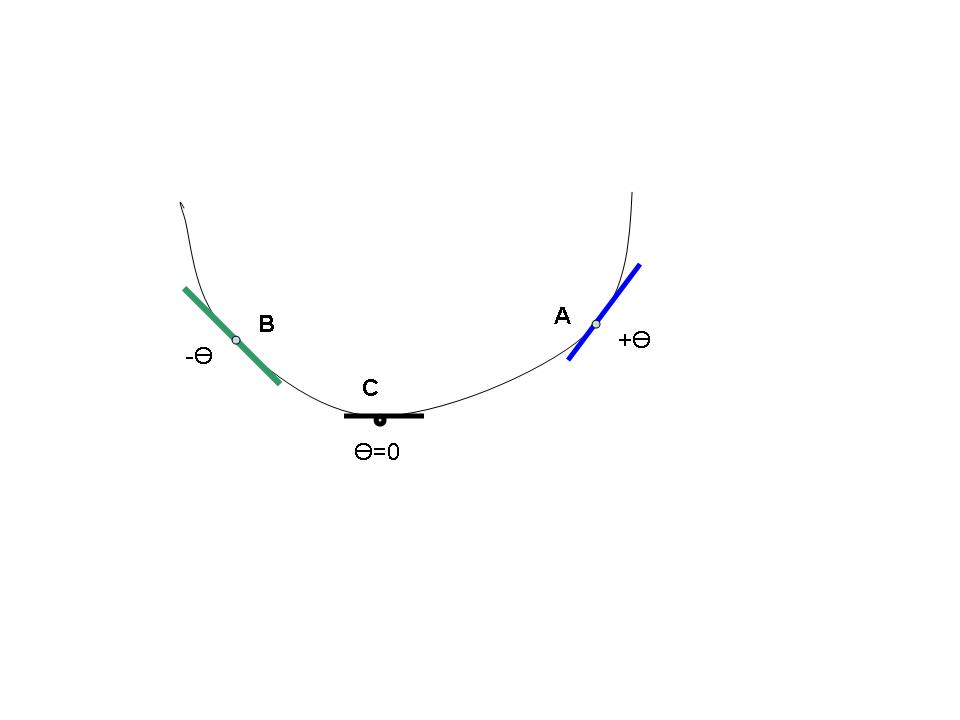
Here is the technique to choose the optimum value for the regularization parameter λ

When λ is small then Ɵ_i values are large and we tend to overfit the data set. Hence the training error will be low but the cross validation error will be high. However when λ is large then the values of Ɵ_ibecome negligible almost leading to a polynomial degree of 1. These will underfit the data and result in a high training error and a cross validation error. Hence the chosen value of λ should be such that the cross validation error is the lowest

Plotting learning curves

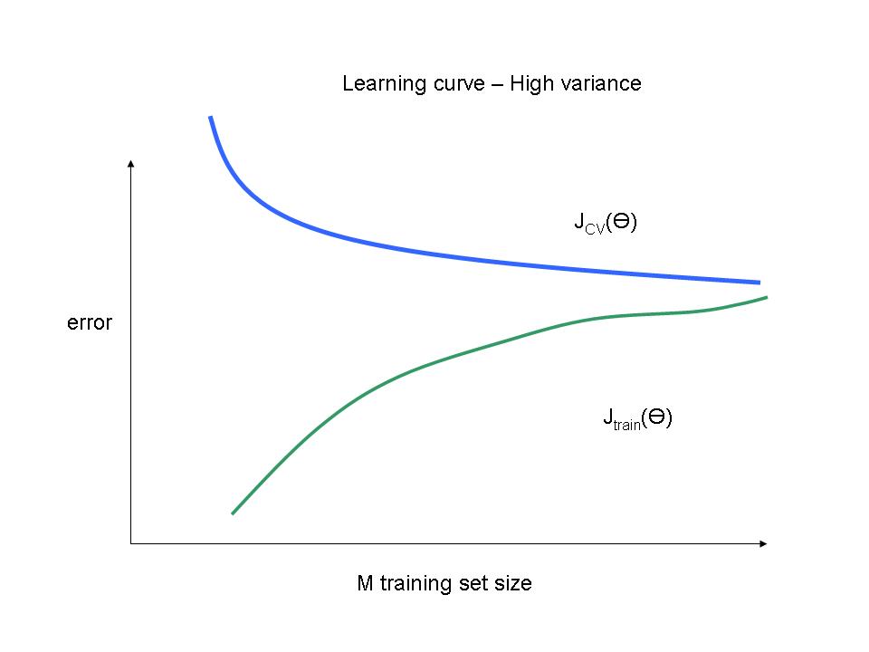
This is another technique to identify if the learned hypothesis has a high bias or a high variance based on the number of training examples

A high bias indicates an underfit. When the number of samples in training set if low then the training error and cross validation error will be low as it will be easy to create a hypothesis if there are few training examples. As the number of samples increase the error will increase for the training set and will slightly decrease for the cross validation set. However for a high bias, or underfit, after a certain point increasing the number of samples will not change the error. This is the case of a high bias

In the case of high variance where a high degree polynomial is used for the hypothesis the training error will be low for smaller number of training examples. As the number of training examples increase the error will increase slowly. The cross validation error will be high for lesser number of training samples but will slowly decrease as the number of samples grow as the hypothesis will learn better. Hence for the case of high variance increasing the number of samples in the training set size will decrease the gap between the cross validation and the training error as shown below

Note: This post, line previous posts on Machine Learning, is based on the Coursera course on Machine Learning by Professor Andrew Ng

Also see
1. My book ‘Practical Machine Learning in R and Python: Third edition’ on Amazon
2.My book ‘Deep Learning from first principles:Second Edition’ now on Amazon
3.The Clash of the Titans in Test and ODI cricket
4. Introducing QCSimulator: A 5-qubit quantum computing simulator in R
5.Latency, throughput implications for the Cloud
6. Simulating a Web Joint in Android
5. Pitching yorkpy … short of good length to IPL – Part 1

Simplifying Machine Learning: Bias, Variance, regularization and odd facts – Part 4

In both linear and logistic regression the choice of the degree of the polynomial for the hypothesis function is extremely critical. A low degree for the polynomial can result in an underfit, while a very high degree can overfit the data as shown below

The figure on the left the data is underfit as we try to fit the data with a first order polynomial which is a straight line. This is a case of strong ‘bias’

The rightmost figure a much higher polynomial is used. All the data points are covered by the polynomial curve however it is not effective in predicting other values. This is a case of overfitting or a high variance.

The middle figure is just right as it intuitively fits the data points the best possible way.

A similar problem exists with logistic regression as shown below

There are 2 ways to handle overfitting

a) Reducing the number of features selected

b) Using regularization

In regularization the magnitude of the parameters Ɵ is decreased to reduce the effect of overfitting

Hence if we choose a hypothesis function

h_Ɵ(x) = Ɵ₀ + Ɵ₁x₁² + Ɵ₂x₂² + Ɵ₃x₃³ + Ɵ₄x₄⁴

The cost function for this without regularization as mentioned in earlier posts

J(Ɵ) = 1/2m Σ(h_Ɵ (xⁱ – yⁱ)²

Where the key is minimize the above function for the least error

The cost function with regularization becomes

J(Ɵ) = 1/2m Σ(h_Ɵ (xⁱ – yⁱ)^{2 +}λ Σ Ɵ_j²

As can be seen the regularization now adds a factor Ɵ_j² as a part of the cost function which needs to be minimized.

Hence with the regularization factor the problem of underfitting/overfitting can be solved

However the trick is determine the value of λ. If λ is too big then it would result in underfitting or resulting in a high bias.

Similarly the regularized equation for logistic regression is as shown below

J(Ɵ) = |1/m Σ -y * log(h_Ɵ(x)) – (1-y) * (log(1 – h_Ɵ(x)) | + λ/2m Σ Ɵ_j²

Some tips suggested by Prof Andrew Ng while determining the parameters and features for regression

a) Get as many training examples. It is worth spending more effort in getting as much examples

b) Add additional features

c) Observe changes to the learning algorithm with different values of λ

This post is continued in my next post – Simplifying ML: Impact of degree of polynomial on bias, variance and other insights

Note: This post, in line with my previous posts on Machine Learning, is based on the Coursera course on Machine Learning by Professor Andrew Ng

Find me on Google+

Simplifying ML: Neural networks- Part 3

Neural networks try to overcome the shortcomings of logistic regression in which we have to choose a non-linear hypothesis. Logistic regression requires that we choose an appropriate combination of polynomial terms and the order of the equation. The problem with this is sometimes we either tend to overfit or underfit. Neural networks allow the ability to learns new model parameters from the basis raw parameters.

The neural network is modeled on the neural networking ability of the human brain. The brain is made of trillions of neurons. Each neuron is a processing unit which has several inputs in the dendrites and an output the axon. The neurons communicate thro a combination of electro chemical signal at the synapses or the spaces between the neuron.

A neural network mimics the working of the neuron.

So in a neural network the features of the problem serve as input. For e.g in the case of being able to determine if a mail is spam or not the features could be the words in the subject line, the from address, the contents etc. Based on a combination of these features we need to classify whether the mail is spam or not.

The above diagram shows a simple neural network with features x₁, x₂, x₃and a bias unit x₀

With a hypothesis function h_Ɵ(x) = 1/(1 + e^-x)

The edges from the features x_i are the model parameters Ɵ. In other words the edges represent weights.

A typical neural network is a network of many logistic units organized in layers. The output of each layer forms the input to the next subsequent layer. This is shown below

As can be seen in a multi-layer neural network at the left we have the features x₁,x₂, .. x_n.

This at the layer becomes the activation unit. The key advantage of neural networks over regular logistic regression that learns the models parameters is that learned model parameters are input to the next subsequent layers which learn the model parameters more finely. Hence this gives a better fit for the combination of parameters.

The activation parameters at the next layer are

a₁² = g(Ɵ₁₀¹x₀+ Ɵ₁₁¹x₁+ Ɵ₁₂¹x₂ + Ɵ₁₃¹x₃) where g is the logistic function or the sigmoid function discussed in my previous post Simplifying ML: Logistic regression – Part 2

Here a₁²is the activation parameter at layer 1

Ɵ₁₀is the model parameter at layer 1 and is the 0^th parameter. Similarly Ɵ₁₁is the model parameter at layer 1 and is the 1^st parameter and so on.

Similarly the other activation parameters can be written as

a₂² = g(Ɵ₂₀¹x₀+ Ɵ₂₁¹x₁+ Ɵ₂₂¹x₂ + Ɵ₂₃¹x₃)

a₃² = g(Ɵ₃₀¹x₀+ Ɵ₃₁¹x₁+ Ɵ₃₂¹x₂ + Ɵ₃₃¹x₃)

h_Ɵ(x) = a₁³ = g(Ɵ₁₀²a₀+ Ɵ₁₁²a₁+ Ɵ₁₂²a₂ + Ɵ₁₃²a₃ – (A)

The crux of neural networks is that instead of creating a hypothesis based on the set of raw features, the neural network with multiple hidden layers can learn its own features. In the equation (A) we can see that the hypothesis is not a function of the input raw features x₁,x₂,… x_nbut on a new set of features or the activation units a₁,a₂, … a_n. In other words the network has ‘learned’ its own features.

As mentioned above the output of each layer is the logistic function or the sigmoid function

The beauty of neural networks based on logistic functions is that we can easily realize the equivalent of logic gates like AND, OR, NOT, NOR etc.

The hypothesis for the above network would be

h_Ɵ(x) = g(-30 + 20 * x₁ + 20 * x₂)

So for x₁= 0 and x₂ = 0 we would have

h_Ɵ(x) = g(-30 + 0 + 0) = g(-30)

Since g(-30) < g(0) < 0.5 = 0

Similarly a NOT gate can be constructed with a neural network as follows

Neural networks can also be used for multi class classification.

Hence there are multiple advantages to neural networks. Neural networks are amenable to a) creating complex logic models of combinations of AND, NOT, OR gates

b) The model parameters are learned from the raw parameters and can be more flexible.

It appears that the interest in neural networks surged in the 1980s and then waned, The neural networks were similar to the above and were based on forward propagation. However it appears that in recent time’s backward propagation has been used successfully in areas of research known as ‘deep learning’

This is based on the Coursera course on Machine Learning by Professor Andrew Ng. A highy enjoyable and classic course!!!

Find me on Google+

Simplifying ML: Logistic regression – Part 2

Logistic regression is another class of Machine Learning algorithms which comes under supervised learning. In this regression technique we need to classify data. Take a look at my earlier post Simplifying Machine Learning algorithms – Part 1 I had discussed linear regression. For e.g if we had data on tumor sizes versus the fact that the tumor was benign or malignant, the question is whether given a tumor size we can predict whether this tumor would be benign or cancerous. So we need to have the ability to classify this data.

This is shown below

It is obvious that a line with a certain slope could easily separate the two.

As another example we could have an algorithm that is able to automatically classify mail as either spam or not spam based on the subject line. So for e.g if the subject line had words like medicine, prize, lottery etc we could with a fair degree of probability classify this as spam.

However some classification problems could be far more complex. We may need to classify another problem as shown below.

From the above it can be seen that hypothesis function is second order equation which is either a circle or an ellipse.

In the case of logistic regression the hypothesis function should be able to switch between 2 values 0 or 1 almost like a transistor either being in cutoff or in saturation state.

In the case of logistic regression 0 <= h_Ɵ<= 1

The hypothesis function uses function of the following form

g(z) = 1/(1 + e^‑z)

and h_Ɵ(x) = g(Ɵ^TX₎

The function g(z) shown above has the characteristic required for logistic regression as it has the following shape

The function rapidly asymptotes at 1 when h_Ɵ(x) >= 0.5 and h_Ɵ(x) asymptotes to 0 when h_Ɵ(x) < 0.5

As in linear regression we can have hypothesis function be of an appropriate order. So for e.g. in the ellipse figure above one could choose a hypothesis function as follows

h_Ɵ(x) = Ɵ₀ + Ɵ₁x₁² + Ɵ₂x₂² + Ɵ₃x₁ + Ɵ₄x₂

h_Ɵ(x) = 1/(1 + e –^{(Ɵ0 + Ɵ1×12 + Ɵ2×22 + Ɵ3×1 + Ɵ4×2)})

We could choose the general form of a circle which is

f(x) = ax² + by² +2gx + 2hy + d

The cost function for logistic regression is given below

Cost(h_Ɵ(x),y) = { -log(h_Ɵ(x)) if y = 1

-log(1 – h_Ɵ(x))) if y = 0

In the case of regression there was a single cost function which could determine the error of the data against the predicted value.

The cost in the event of logistic regression is given as above as a set of 2 equations one for the case where the data is 1 and another for the case where the data is 0.

The reason for this is as follows. If we consider y =1 as a positive value, then when our hypothesis correctly predicts 1 then we have a ‘true positive’ however if we predict 0 when it should be 1 then we have a false negative. Similarly when the data is 0 and we predict a 1 then this is the case of a false positive and if we correctly predict 0 when it is 0 it is true negative.

Here is the reason as how the cost function

Cost(h_Ɵ(x),y) = { -log(h_Ɵ(x)) if y = 1

-log(1 – h_Ɵ(x))) if y = 0

Was arrived at. By definition the cost function gives the error between the predicted value and the data value.

The logic for determining the appropriate function is as follows

For y = 1

y=1 & hypothesis = 1 then cost = 0

y= 1 & hypothesis = 0 then cost = Infinity

Similarly for y = 0

y = 0 & hypotheses = 0 then cost = 0

y = 0 & hypothesis = 1 then cost = Infinity

and the the functions above serve exactly this purpose as can be seen

Hence the cost can be written as

J(Ɵ) = Cost(h_Ɵ(x),y) = -y * log(h_Ɵ(x)) – (1-y) * (log(1 – h_Ɵ(x))

This is the same as the equation above

The same gradient descent algorithm can now be used to minimize the cost function

So we can iterate througj

Ɵ_j = Ɵ_j – α δ/δ Ɵ_j J(Ɵ₀, Ɵ₁,… Ɵ_n)

This works out to a function that is similar to linear regression

Ɵj₌Ɵj – α 1/m { Σ h_Ɵ(x_i) – y_i} x_jⁱ

This will enable the machine to fairly accurately determine the parameters Ɵ_jfor the features x and provide the hypothesis function.

This is based on the Coursera course on Machine Learning by Professor Andrew Ng. Highly recommended!!!

Find me on Google+

Simplifying Machine Learning algorithms – Part 1

Machine learning or the ability to use computers to predict values, classify data or identify patterns is truly a fascinating field. It is amazing how algorithms can come to conclusions on data. Detecting patterns is a inborn ability of the human mind. But our mind cannot handle large quantities of data with many features. It is here that machines have an edge over us.

This post is inspired by the Machine Learning course at Coursera conducted by Professor Andrew Ng of Stanford. The lectures are truly lucid and delivered with amazing clarity. In a series of post I will be trying to distil the meaning and motivation behind the algorithms that are part of machine learning.

There are 2 major types of learning

a) Supervised learning b) Unsupervised learning

Supervised learning: In supervised learning we have to infer the relationship between input data and output values. The intention of supervised learning is determine the possible out for some random input once the relationship has been determined. Some examples of supervised learning are linear regression, logistic regression etc.

Unsupervised learning: In unsupervised learning the problem is to determine patterns and structure in unlabeled data. Some examples of unsupervised learning are K-Means clustering, hidden Markov models etc.

In this post I would like to take a look at Supervised Learning algorithms

Linear Regression

In regression problems we try to infer the relationship between a set of input parameters to an output value. Let us we have data for the number of rooms vs. price of the house as shown below

Depending on the data we could either fit a straight line or use a linear fit. Alternatively we could fit a higher order curve to data.

The function that determines the relationship is also known as hypothesis function. This can be represented as follows for e.g a hypothesis function with a single feature

h_Ɵ(x) = Ɵ₁x+ Ɵ₀

The above equation is the hypothesis function where Ɵ is the parameter and x is the feature

We could have a higher order hypothesis function as follows

h_Ɵ(x) = Ɵ₂x²+ Ɵ₁x+Ɵ₀

To evaluate whether the hypothesis function is able to map the input and related output accurately is known as the ‘cost function’.

The cost function can be represented as

J(Ɵ) = 1/2m Σ(h_Ɵ (xⁱ)– yⁱ)²

The cost function really calculates the ‘mean squared error’ of the actual data points (y) with the points on the hypothesis function (h_Ɵ). Clearly higher the value of J(Ɵ) the greater is the error in predicting the output based on a set of input parameters. If we just took the error instead of the squared error then if there were data points on either side of the predicted line then the positive & negative errors could cancel out. Hence the approach is usually to take the mean of the squared error.

The goal would be to minimize the error which will result in the best fit.

So the approach would be to choose values for the parameters Ɵi

The algorithm that is used for determining the values of the parameters that will result in the minimum error is gradient descent

The formula is

Ɵj := Ɵj – αd/d Ɵj J(Ɵ)

Where α is the learning rate

Gradient descent starts by picking a random value for Ɵi. Then the algorithm looks around to search for the next combination that will take us down fastest. By continuing this process the local minima is determined.

Gradient descent is based on the observation that if the multivariable function is defined and differentiable in a neighborhood of a point , then decreases fastest if one goes from in the direction of the negative gradient. This is shown in the below diagram taken from Wikipedia.

For e.g for a curve as shown below

This how I think the gradient descent works. In the above diagram at point A the slope is +ve and taking the negative of the slope multiplied by the learning factor α and subtracting it from Ɵj will result in a value that is less than Ɵj. That is we move towards the minima or C. Similarly at point B the slope will be -ve. If we multiply by – α then we will add to Ɵj. Hence we will move to the right or towards point C.

By applying the iterative process of gradient descent we can get the combination of parameter values for Ɵ that will provide the best fit for the set of data points

The iterative process of gradient descent is applied to minimize the cost function which is function of the error in the current hypothesis

δ/δ J(Ɵ) = δ/ δ Ɵ * 1/2m Σ(h_Ɵ (xⁱ)– yⁱ)²

This process is applied iteratively to the below equation to arrive at the values of Ɵi

The formula is

Ɵj := Ɵj – αd/d Ɵj J(Ɵ)

to obtain the values for the best fit equation

h_Ɵ(x) = Ɵ₂xⁿ+ Ɵ₁x^n-1+ …+ Ɵ₀

Also read my post on Simplifying ML: Logistic regression – Part 2

Find me on Google+