Are you wondering whether to get into the ‘R’ bus or ‘Python’ bus? My suggestion is to you is “Why not get into the ‘R and Python’ train?”
The third edition of my book ‘Practical Machine Learning with R and Python – Machine Learning in stereo’ is now available in both paperback ($12.99) and kindle ($8.99/Rs449) versions. In the third edition all code sections have been re-formatted to use the fixed width font ‘Consolas’. This neatly organizes output which have columns like confusion matrix, dataframes etc to be columnar, making the code more readable. There is a science to formatting too!! which improves the look and feel. It is little wonder that Steve Jobs had a keen passion for calligraphy! Additionally some typos have been fixed.
This book is ideal both for beginners and the experts in R and/or Python. Those starting their journey into datascience and ML will find the first 3 chapters useful, as they touch upon the most important programming constructs in R and Python and also deal with equivalent statements in R and Python. Those who are expert in either of the languages, R or Python, will find the equivalent code ideal for brushing up on the other language. And finally,those who are proficient in both languages, can use the R and Python implementations to internalize the ML algorithms better.
Here is a look at the topics covered
Table of Contents
Preface …………………………………………………………………………….4
Introduction ………………………………………………………………………6
1. Essential R ………………………………………………………………… 8
2. Essential Python for Datascience ……………………………………………57
3. R vs Python …………………………………………………………………81
4. Regression of a continuous variable ……………………………………….101
5. Classification and Cross Validation ………………………………………..121
6. Regression techniques and regularization ………………………………….146
7. SVMs, Decision Trees and Validation curves ………………………………191
8. Splines, GAMs, Random Forests and Boosting ……………………………222
9. PCA, K-Means and Hierarchical Clustering ………………………………258
References ……………………………………………………………………..269
Pick up your copy today!!
Hope you have a great time learning as I did while implementing these algorithms!
The second edition of my book ‘Deep Learning from first principles:Second Edition- In vectorized Python, R and Octave’, is now available on Amazon, in both paperback ($18.99) and kindle ($9.99/Rs449/-) versions. Since this book is almost 70% code, all functions, and code snippets have been formatted to use the fixed-width font ‘Lucida Console’. In addition line numbers have been added to all code snippets. This makes the code more organized and much more readable. I have also fixed typos in the book
This presentation is a continuation of my earlier presentation Presentation on ‘Machine Learning in plain English – Part 1’. As the title suggests, the presentation is devoid of any math or programming constructs, and just focuses on the concepts and approaches to different Machine Learning algorithms. In this 2nd part, I discuss KNN regression, KNN classification, Cross Validation techniques like (LOOCV, K-Fold) feature selection methods including best-fit,forward-fit and backward fit and finally Ridge (L2) and Lasso Regression (L1)
This is the first part on my series ‘Machine Learning in plain English – Part 1’ in which I discuss the intuition behind different Machine Learning algorithms, metrics and the approaches etc. These presentations will not include tiresome math or laborious programming constructs, and will instead focus on just the concepts behind the Machine Learning algorithms. This presentation discusses what Machine Learning is, Gradient Descent, linear, multi variate & polynomial regression, bias/variance, under fit, good fit and over fit and finally logistic regression etc.
It is hoped that these presentations will trigger sufficient interest in you, to explore this fascinating field further
My book ‘Practical Machine Learning with R and Python: Second Edition – Machine Learning in stereo’ is now available in both paperback ($10.99) and kindle ($7.99/Rs449) versions. In this book I implement some of the most common, but important Machine Learning algorithms in R and equivalent Python code. This is almost like listening to parallel channels of music in stereo!
1. Practical machine with R and Python: Third Edition – Machine Learning in Stereo(Paperback-$12.99)
2. Practical machine with R and Python Third Edition – Machine Learning in Stereo(Kindle- $8.99/Rs449)
This book is ideal both for beginners and the experts in R and/or Python. Those starting their journey into datascience and ML will find the first 3 chapters useful, as they touch upon the most important programming constructs in R and Python and also deal with equivalent statements in R and Python. Those who are expert in either of the languages, R or Python, will find the equivalent code ideal for brushing up on the other language. And finally,those who are proficient in both languages, can use the R and Python implementations to internalize the ML algorithms better.
Here is a look at the topics covered
Table of Contents
Essential R …………………………………….. 7
Essential Python for Datascience ……………….. 54
R vs Python ……………………………………. 77
Regression of a continuous variable ………………. 96
Classification and Cross Validation ……………….113
Regression techniques and regularization …………. 134
SVMs, Decision Trees and Validation curves …………175
Splines, GAMs, Random Forests and Boosting …………202
PCA, K-Means and Hierarchical Clustering …………. 234
Pick up your copy today!!
Hope you have a great time learning as I did while implementing these algorithms!
This is the 5th and probably penultimate part of my series on ‘Practical Machine Learning with R and Python’. The earlier parts of this series included
This post ‘Practical Machine Learning with R and Python – Part 5’ discusses regression with B-splines, natural splines, smoothing splines, generalized additive models (GAMS), bagging, random forest and boosting
As with my previous posts in this series, this post is largely based on the following 2 MOOC courses
Check out my compact and minimal book “Practical Machine Learning with R and Python:Third edition- Machine Learning in stereo” available in Amazon in paperback($12.99) and kindle($8.99) versions. My book includes implementations of key ML algorithms and associated measures and metrics. The book is ideal for anybody who is familiar with the concepts and would like a quick reference to the different ML algorithms that can be applied to problems and how to select the best model. Pick your copy today!!
When performing regression (continuous or logistic) between a target variable and a feature (or a set of features), a single polynomial for the entire range of the data set usually does not perform a good fit.Rather we would need to provide we could fit
regression curves for different section of the data set.
There are several techniques which do this for e.g. piecewise-constant functions, piecewise-linear functions, piecewise-quadratic/cubic/4th order polynomial functions etc. One such set of functions are the cubic splines which fit cubic polynomials to successive sections of the dataset. The points where the cubic splines join, are called ‘knots’.
Since each section has a different cubic spline, there could be discontinuities (or breaks) at these knots. To prevent these discontinuities ‘natural splines’ and ‘smoothing splines’ ensure that the seperate cubic functions have 2nd order continuity at these knots with the adjacent splines. 2nd order continuity implies that the value, 1st order derivative and 2nd order derivative at these knots are equal.
A cubic spline with knots , k=1,2,3,..K is a piece-wise cubic polynomial with continuous derivative up to order 2 at each knot. We can write .
For each (), are called ‘basis’ functions, where , , , where k=1,2,3… K The 1st and 2nd derivatives of cubic splines are continuous at the knots. Hence splines provide a smooth continuous fit to the data by fitting different splines to different sections of the data
1.1a Fit a 4th degree polynomial – R code
In the code below a non-linear function (a 4th order polynomial) is used to fit the data. Usually when we fit a single polynomial to the entire data set the tails of the fit tend to vary a lot particularly if there are fewer points at the ends. Splines help in reducing this variation at the extremities
library(dplyr)library(ggplot2)source('RFunctions-1.R')# Read the datadf=read.csv("auto_mpg.csv",stringsAsFactors=FALSE)# Data from UCIdf1<-as.data.frame(sapply(df,as.numeric))#Select specific columnsdf2<-df1%>%dplyr::select(cylinder,displacement, horsepower,weight, acceleration, year,mpg)auto<-df2[complete.cases(df2),]# Fit a 4th degree polynomialfit=lm(mpg~poly(horsepower,4),data=auto)#Display a summary of fitsummary(fit)
#Get the range of horsepowerhp<-range(auto$horsepower)#Create a sequence to be used for plottinghpGrid<-seq(hp[1],hp[2],by=10)#Predict for these values of horsepower. Set Standard error as TRUEpred=predict(fit,newdata=list(horsepower=hpGrid),se=TRUE)#Compute bands on either side that is 2xSEseBands=cbind(pred$fit+2*pred$se.fit,pred$fit-2*pred$se.fit)#Plot the fit with Standard Error bandsplot(auto$horsepower,auto$mpg,xlim=hp,cex=.5,col="black",xlab="Horsepower",
ylab="MPG", main="Polynomial of degree 4")lines(hpGrid,pred$fit,lwd=2,col="blue")matlines(hpGrid,seBands,lwd=2,col="blue",lty=3)
1.1b Fit a 4th degree polynomial – Python code
import numpy as np
import pandas as pd
import os
import matplotlib.pyplot as plt
from sklearn.model_selection import train_test_split
from sklearn.preprocessing import PolynomialFeatures
from sklearn.linear_model import LinearRegression
#Read the auto data
autoDF =pd.read_csv("auto_mpg.csv",encoding="ISO-8859-1")
# Select columns
autoDF1=autoDF[['mpg','cylinder','displacement','horsepower','weight','acceleration','year']]
# Convert all columns to numeric
autoDF2 = autoDF1.apply(pd.to_numeric, errors='coerce')

#Drop NAs
autoDF3=autoDF2.dropna()
autoDF3.shape
X=autoDF3[['horsepower']]
y=autoDF3['mpg']
#Create a polynomial of degree 4
poly = PolynomialFeatures(degree=4)
X_poly = poly.fit_transform(X)

# Fit a polynomial regression line
linreg = LinearRegression().fit(X_poly, y)
# Create a range of values
hpGrid = np.arange(np.min(X),np.max(X),10)
hp=hpGrid.reshape(-1,1)
# Transform to 4th degree
poly = PolynomialFeatures(degree=4)
hp_poly = poly.fit_transform(hp)

#Create a scatter plot
plt.scatter(X,y)
# Fit the prediction
ypred=linreg.predict(hp_poly)
plt.title("Poylnomial of degree 4")
fig2=plt.xlabel("Horsepower")
fig2=plt.ylabel("MPG")
# Draw the regression curve
plt.plot(hp,ypred,c="red")
plt.savefig('fig1.png', bbox_inches='tight')
1.1c Fit a B-Spline – R Code
In the code below a B- Spline is fit to data. The B-spline requires the manual selection of knots
#Splineslibrary(splines)# Fit a B-spline to the data. Select knots at 60,75,100,150fit=lm(mpg~bs(horsepower,df=6,knots=c(60,75,100,150)),data=auto)# Use the fitted regresion to predictpred=predict(fit,newdata=list(horsepower=hpGrid),se=T)# Create a scatter plotplot(auto$horsepower,auto$mpg,xlim=hp,cex=.5,col="black",xlab="Horsepower",
ylab="MPG", main="B-Spline with 4 knots")#Draw lines with 2 Standard Errors on either sidelines(hpGrid,pred$fit,lwd=2)lines(hpGrid,pred$fit+2*pred$se,lty="dashed")lines(hpGrid,pred$fit-2*pred$se,lty="dashed")abline(v=c(60,75,100,150),lty=2,col="darkgreen")
1.1d Fit a Natural Spline – R Code
Here a ‘Natural Spline’ is used to fit .The Natural Spline extrapolates beyond the boundary knots and the ends of the function are much more constrained than a regular spline or a global polynomoial where the ends can wag a lot more. Natural splines do not require the explicit selection of knots
# There is no need to select the knots here. There is a smoothing parameter which# can be specified by the degrees of freedom 'df' parameter. The natural splinefit2=lm(mpg~ns(horsepower,df=4),data=auto)pred=predict(fit2,newdata=list(horsepower=hpGrid),se=T)plot(auto$horsepower,auto$mpg,xlim=hp,cex=.5,col="black",xlab="Horsepower",
ylab="MPG", main="Natural Splines")lines(hpGrid,pred$fit,lwd=2)lines(hpGrid,pred$fit+2*pred$se,lty="dashed")lines(hpGrid,pred$fit-2*pred$se,lty="dashed")
1.1.e Fit a Smoothing Spline – R code
Here a smoothing spline is used. Smoothing splines also do not require the explicit setting of knots. We can change the ‘degrees of freedom(df)’ paramater to get the best fit
# Smoothing spline has a smoothing parameter, the degrees of freedom# This is too wigglyplot(auto$horsepower,auto$mpg,xlim=hp,cex=.5,col="black",xlab="Horsepower",
ylab="MPG", main="Smoothing Splines")# Here df is set to 16. This has a lot of variancefit=smooth.spline(auto$horsepower,auto$mpg,df=16)lines(fit,col="red",lwd=2)# We can use Cross Validation to allow the spline to pick the value of this smpopothing paramter. We do not need to set the degrees of freedom 'df'fit=smooth.spline(auto$horsepower,auto$mpg,cv=TRUE)lines(fit,col="blue",lwd=2)
1.1e Splines – Python
There isn’t as much treatment of splines in Python and SKLearn. I did find the LSQUnivariate, UnivariateSpline spline. The LSQUnivariate spline requires the explcit setting of knots
import numpy as np
import pandas as pd
import os
import matplotlib.pyplot as plt
from scipy.interpolate import LSQUnivariateSpline
autoDF =pd.read_csv("auto_mpg.csv",encoding="ISO-8859-1")
autoDF.shape
autoDF.columns
autoDF1=autoDF[['mpg','cylinder','displacement','horsepower','weight','acceleration','year']]
autoDF2 = autoDF1.apply(pd.to_numeric, errors='coerce')
auto=autoDF2.dropna()
auto=auto[['horsepower','mpg']].sort_values('horsepower')

# Set the knots manually
knots=[65,75,100,150]
# Create an array for X & y
X=np.array(auto['horsepower'])
y=np.array(auto['mpg'])
# Fit a LSQunivariate spline
s = LSQUnivariateSpline(X,y,knots)

#Plot the spline
xs = np.linspace(40,230,1000)
ys = s(xs)
plt.scatter(X, y)
plt.plot(xs, ys)
plt.savefig('fig2.png', bbox_inches='tight')
1.2 Generalized Additiive models (GAMs)
Generalized Additive Models (GAMs) is a really powerful ML tool.
In GAMs we use a different functions for each of the variables. GAMs give a much better fit since we can choose any function for the different sections
1.2a Generalized Additive Models (GAMs) – R Code
The plot below show the smooth spline that is fit for each of the features horsepower, cylinder, displacement, year and acceleration. We can use any function for example loess, 4rd order polynomial etc.
library(gam)# Fit a smoothing spline for horsepower, cyliner, displacement and accelerationgam=gam(mpg~s(horsepower,4)+s(cylinder,5)+s(displacement,4)+s(year,4)+s(acceleration,5),data=auto)# Display the summary of the fit. This give the significance of each of the paramwetr# Also an ANOVA is given for each combination of the featuressummary(gam)
I did not find the equivalent of GAMs in SKlearn in Python. There was an early prototype (2012) in Github. Looks like it is still work in progress or has probably been abandoned.
1.3 Tree based Machine Learning Models
Tree based Machine Learning are all based on the ‘bootstrapping’ technique. In bootstrapping given a sample of size N, we create datasets of size N by sampling this original dataset with replacement. Machine Learning models are built on the different bootstrapped samples and then averaged.
Decision Trees as seen above have the tendency to overfit. There are several techniques that help to avoid this namely a) Bagging b) Random Forests c) Boosting
Bagging, Random Forest and Gradient Boosting
Bagging: Bagging, or Bootstrap Aggregation decreases the variance of predictions, by creating separate Decisiion Tree based ML models on the different samples and then averaging these ML models
Random Forests: Bagging is a greedy algorithm and tries to produce splits based on all variables which try to minimize the error. However the different ML models have a high correlation. Random Forests remove this shortcoming, by using a variable and random set of features to split on. Hence the features chosen and the resulting trees are uncorrelated. When these ML models are averaged the performance is much better.
Boosting: Gradient Boosted Decision Trees also use an ensemble of trees but they don’t build Machine Learning models with random set of features at each step. Rather small and simple trees are built. Successive trees try to minimize the error from the earlier trees.
Out of Bag (OOB) Error: In Random Forest and Gradient Boosting for each bootstrap sample taken from the dataset, there will be samples left out. These are known as Out of Bag samples.Classification accuracy carried out on these OOB samples is known as OOB error
1.31a Decision Trees – R Code
The code below creates a Decision tree with the cancer training data. The summary of the fit is output. Based on the ML model, the predict function is used on test data and a confusion matrix is output.
# Read the cancer datalibrary(tree)library(caret)library(e1071)cancer<-read.csv("cancer.csv",stringsAsFactors=FALSE)cancer<-cancer[,2:32]cancer$target<-as.factor(cancer$target)train_idx<-trainTestSplit(cancer,trainPercent=75,seed=5)train<-cancer[train_idx, ]test<-cancer[-train_idx, ]# Create Decision TreecancerStatus=tree(target~.,train)summary(cancerStatus)
##
## Classification tree:
## tree(formula = target ~ ., data = train)
## Variables actually used in tree construction:
## [1] "worst.perimeter"      "worst.concave.points" "area.error"
## [4] "worst.texture"        "mean.texture"         "mean.concave.points"
## Number of terminal nodes:  9
## Residual mean deviance:  0.1218 = 50.8 / 417
## Misclassification error rate: 0.02347 = 10 / 426
Below is the Python code for creating Decision Trees. The accuracy, precision, recall and F1 score is computed on the test data set.
import numpy as np
import pandas as pd
import os
import matplotlib.pyplot as plt
from sklearn.metrics import confusion_matrix
from sklearn import tree
from sklearn.datasets import load_breast_cancer
from sklearn.model_selection import train_test_split
from sklearn.tree import DecisionTreeClassifier
from sklearn.datasets import make_classification, make_blobs
from sklearn.metrics import accuracy_score, precision_score, recall_score, f1_score
import graphviz

cancer = load_breast_cancer()
(X_cancer, y_cancer) = load_breast_cancer(return_X_y = True)

X_train, X_test, y_train, y_test = train_test_split(X_cancer, y_cancer,
                                                   random_state = 0)
clf = DecisionTreeClassifier().fit(X_train, y_train)

print('Accuracy of Decision Tree classifier on training set: {:.2f}'
     .format(clf.score(X_train, y_train)))
print('Accuracy of Decision Tree classifier on test set: {:.2f}'
     .format(clf.score(X_test, y_test)))

y_predicted=clf.predict(X_test)
confusion = confusion_matrix(y_test, y_predicted)
print('Accuracy: {:.2f}'.format(accuracy_score(y_test, y_predicted)))
print('Precision: {:.2f}'.format(precision_score(y_test, y_predicted)))
print('Recall: {:.2f}'.format(recall_score(y_test, y_predicted)))
print('F1: {:.2f}'.format(f1_score(y_test, y_predicted)))

# Plot the Decision Tree
clf = DecisionTreeClassifier(max_depth=2).fit(X_train, y_train)
dot_data = tree.export_graphviz(clf, out_file=None,
                         feature_names=cancer.feature_names,
                         class_names=cancer.target_names,
                         filled=True, rounded=True,
                         special_characters=True)
graph = graphviz.Source(dot_data)
graph
## Accuracy of Decision Tree classifier on training set: 1.00
## Accuracy of Decision Tree classifier on test set: 0.87
## Accuracy: 0.87
## Precision: 0.97
## Recall: 0.82
## F1: 0.89
1.31d Decision Trees – Cross Validation – Python Code
In the code below 5-fold cross validation is performed for different depths of the tree and the accuracy is computed. The accuracy on the test set seems to plateau when the depth is 8. But it is seen to increase again from 10 to 12. More analysis needs to be done here
import numpy as np
import pandas as pd
import os
import matplotlib.pyplot as plt
from sklearn.datasets import load_breast_cancer
from sklearn.tree import DecisionTreeClassifier
(X_cancer, y_cancer) = load_breast_cancer(return_X_y = True)
from sklearn.cross_validation import train_test_split, KFold
defcomputeCVAccuracy(X,y,folds):
accuracy=[]
foldAcc=[]
depth=[1,2,3,4,5,6,7,8,9,10,11,12]
nK=len(X)/float(folds)
xval_err=0for i in depth:
kf = KFold(len(X),n_folds=folds)
for train_index, test_index in kf:
X_train, X_test = X.iloc[train_index], X.iloc[test_index]
y_train, y_test = y.iloc[train_index], y.iloc[test_index]
clf = DecisionTreeClassifier(max_depth = i).fit(X_train, y_train)
score=clf.score(X_test, y_test)
accuracy.append(score)
foldAcc.append(np.mean(accuracy))
return(foldAcc)
cvAccuracy=computeCVAccuracy(pd.DataFrame(X_cancer),pd.DataFrame(y_cancer),folds=10)
df1=pd.DataFrame(cvAccuracy)
df1.columns=['cvAccuracy']
df=df1.reindex([1,2,3,4,5,6,7,8,9,10,11,12])
df.plot()
plt.title("Decision Tree - 10-fold Cross Validation Accuracy vs Depth of tree")
plt.xlabel("Depth of tree")
plt.ylabel("Accuracy")
plt.savefig('fig3.png', bbox_inches='tight')
1.4a Random Forest – R code
A Random Forest is fit using the Boston data. The summary shows that 4 variables were randomly chosen at each split and the resulting ML model explains 88.72% of the test data. Also the variable importance is plotted. It can be seen that ‘rooms’ and ‘status’ are the most influential features in the model
library(randomForest)df=read.csv("Boston.csv",stringsAsFactors=FALSE)# Data from MASS - SL# Select specific columnsBoston<-df%>%dplyr::select("crimeRate","zone","indus","charles","nox","rooms","age", "distances","highways","tax","teacherRatio","color",
"status","medianValue")# Fit a Random Forest on the Boston training datarfBoston=randomForest(medianValue~.,data=Boston)# Display the summatu of the fit. It can be seen that the MSE is 10.88 # and the percentage variance explained is 86.14%. About 4 variables were tried at each # #split for a maximum tree of 500.# The MSE and percent variance is on Out of Bag treesrfBoston
##
## Call:
##  randomForest(formula = medianValue ~ ., data = Boston)
##                Type of random forest: regression
##                      Number of trees: 500
## No. of variables tried at each split: 4
##
##           Mean of squared residuals: 9.521672
##                     % Var explained: 88.72
#List and plot the variable importancesimportance(rfBoston)
##              IncNodePurity
## crimeRate        2602.1550
## zone              258.8057
## indus            2599.6635
## charles           240.2879
## nox              2748.8485
## rooms           12011.6178
## age              1083.3242
## distances        2432.8962
## highways          393.5599
## tax              1348.6987
## teacherRatio     2841.5151
## color             731.4387
## status          12735.4046
varImpPlot(rfBoston)
1.4b Random Forest-OOB and Cross Validation Error – R code
The figure below shows the OOB error and the Cross Validation error vs the ‘mtry’. Here mtry indicates the number of random features that are chosen at each split. The lowest test error occurs when mtry = 8
library(randomForest)df=read.csv("Boston.csv",stringsAsFactors=FALSE)# Data from MASS - SL# Select specific columnsBoston<-df%>%dplyr::select("crimeRate","zone","indus","charles","nox","rooms","age", "distances","highways","tax","teacherRatio","color",
"status","medianValue")# Split as training and tst setstrain_idx<-trainTestSplit(Boston,trainPercent=75,seed=5)train<-Boston[train_idx, ]test<-Boston[-train_idx, ]#Initialize OOD and testErroroobError<-NULLtestError<-NULL# In the code below the number of variables to consider at each split is increased# from 1 - 13(max features) and the OOB error and the MSE is computedfor(iin1:13){fitRF=randomForest(medianValue~.,data=train,mtry=i,ntree=400)oobError[i]<-fitRF$mse[400]pred<-predict(fitRF,newdata=test)testError[i]<-mean((pred-test$medianValue)^2)}# We can see the OOB and Test Error. It can be seen that the Random Forest performs# best with the lowers MSE at mtry=6matplot(1:13,cbind(testError,oobError),pch=19,col=c("red","blue"),
type="b",xlab="mtry(no of varaibles at each split)", ylab="Mean Squared Error",
main="Random Forest - OOB and Test Error")legend("topright",legend=c("OOB","Test"),pch=19,col=c("red","blue"))
1.4c Random Forest – Python code
The python code for Random Forest Regression is shown below. The training and test score is computed. The variable importance shows that ‘rooms’ and ‘status’ are the most influential of the variables
1.4d Random Forest – Cross Validation and OOB Error – Python code
As with R the ‘max_features’ determines the random number of features the random forest will use at each split. The plot shows that when max_features=8 the MSE is lowest
import numpy as np
import pandas as pd
import os
import matplotlib.pyplot as plt
from sklearn.model_selection import train_test_split
from sklearn.ensemble import RandomForestRegressor
from sklearn.model_selection import cross_val_score
df = pd.read_csv("Boston.csv",encoding = "ISO-8859-1")

X=df[['crimeRate','zone', 'indus','charles','nox','rooms', 'age','distances','highways','tax',
       'teacherRatio','color','status']]
y=df['medianValue']

cvError=[]
oobError=[]
oobMSE=[]
for i in range(1,13):
    regr = RandomForestRegressor(max_depth=4, n_estimators=400,max_features=i,oob_score=True,random_state=0)
    mse= np.mean(cross_val_score(regr, X, y, cv=5,scoring = 'neg_mean_squared_error'))
    # Since this is neg_mean_squared_error I have inverted the sign to get MSE
    cvError.append(-mse)
    # Fit on all data to compute OOB error
    regr.fit(X, y)
    # Record the OOB error for each `max_features=i` setting
    oob = 1 - regr.oob_score_
    oobError.append(oob)
    # Get the Out of Bag prediction
    oobPred=regr.oob_prediction_
    # Compute the Mean Squared Error between OOB Prediction and target
    mseOOB=np.mean(np.square(oobPred-y))
    oobMSE.append(mseOOB)

# Plot the CV Error and OOB Error
# Set max_features
maxFeatures=np.arange(1,13)
cvError=pd.DataFrame(cvError,index=maxFeatures)
oobMSE=pd.DataFrame(oobMSE,index=maxFeatures)
#Plot
fig8=df.plot()
fig8=plt.title('Random forest - CV Error and OOB Error vs max_features')
fig8.figure.savefig('fig8.png', bbox_inches='tight')

#Plot the OOB Error vs max_features
plt.plot(range(1,13),oobError)
fig2=plt.title("Random Forest - OOB Error vs max_features (variable no of features)")
fig2=plt.xlabel("max_features (variable no of features)")
fig2=plt.ylabel("OOB Error")
fig2.figure.savefig('fig7.png', bbox_inches='tight')
1.5a Boosting – R code
Here a Gradient Boosted ML Model is built with a n.trees=5000, with a learning rate of 0.01 and depth of 4. The feature importance plot also shows that rooms and status are the 2 most important features. The MSE vs the number of trees plateaus around 2000 trees
library(gbm)# Perform gradient boosting on the Boston data set. The distribution is gaussian since we# doing MSE. The interaction depth specifies the number of splitsboostBoston=gbm(medianValue~.,data=train,distribution="gaussian",n.trees=5000,
shrinkage=0.01,interaction.depth=4)#The summary gives the variable importance. The 2 most significant variables are# number of rooms and lower statussummary(boostBoston)
##                       var    rel.inf
## rooms               rooms 42.2267200
## status             status 27.3024671
## distances       distances  7.9447972
## crimeRate       crimeRate  5.0238827
## nox                   nox  4.0616548
## teacherRatio teacherRatio  3.1991999
## age                   age  2.7909772
## color               color  2.3436295
## tax                   tax  2.1386213
## charles           charles  1.3799109
## highways         highways  0.7644026
## indus               indus  0.7236082
## zone                 zone  0.1001287
# The plots below show how each variable relates to the median value of the home. As# the number of roomd increase the median value increases and with increase in lower status# the median value decreasespar(mfrow=c(1,2))#Plot the relation between the top 2 features and the targetplot(boostBoston,i="rooms")plot(boostBoston,i="status")
# Create a sequence of trees between 100-5000 incremented by 50nTrees=seq(100,5000,by=50)# Predict the values for the test datapred<-predict(boostBoston,newdata=test,n.trees=nTrees)# Compute the mean for each of the MSE for each of the number of trees boostError<-apply((pred-test$medianValue)^2,2,mean)#Plot the MSE vs the number of treesplot(nTrees,boostError,pch=19,col="blue",ylab="Mean Squared Error",
main="Boosting Test Error")
1.5b Cross Validation Boosting – R code
Included below is a cross validation error vs the learning rate. The lowest error is when learning rate = 0.09
cvError<-NULLs<-c(.001,0.01,0.03,0.05,0.07,0.09,0.1)for(iinseq_along(s)){cvBoost=gbm(medianValue~.,data=train,distribution="gaussian",n.trees=5000,
shrinkage=s[i],interaction.depth=4,cv.folds=5)cvError[i]<-mean(cvBoost$cv.error)}# Create a data frame for plottinga<-rbind(s,cvError)b<-as.data.frame(t(a))# It can be seen that a shrinkage parameter of 0,05 gives the lowes CV Errorggplot(b,aes(s,cvError))+geom_point()+geom_line(color="blue")+xlab("Shrinkage")+ylab("Cross Validation Error")+ggtitle("Gradient boosted trees - Cross Validation error vs Shrinkage")
1.5c Boosting – Python code
A gradient boost ML model in Python is created below. The Rsquared score is computed on the training and test data.
import numpy as np
import pandas as pd
import os
import matplotlib.pyplot as plt
from sklearn.model_selection import train_test_split
from sklearn.ensemble import GradientBoostingRegressor
df = pd.read_csv("Boston.csv",encoding = "ISO-8859-1")

X=df[['crimeRate','zone', 'indus','charles','nox','rooms', 'age','distances','highways','tax',
       'teacherRatio','color','status']]
y=df['medianValue']

X_train, X_test, y_train, y_test = train_test_split(X, y, random_state = 0)

regr = GradientBoostingRegressor()
regr.fit(X_train, y_train)

print('R-squared score (training): {:.3f}'
     .format(regr.score(X_train, y_train)))
print('R-squared score (test): {:.3f}'
     .format(regr.score(X_test, y_test)))
the cross validation error is computed as the learning rate is varied. The minimum CV eror occurs when lr = 0.04
import numpy as np
import pandas as pd
import os
import matplotlib.pyplot as plt
from sklearn.model_selection import train_test_split
from sklearn.ensemble import RandomForestRegressor
from sklearn.ensemble import GradientBoostingRegressor
from sklearn.model_selection import cross_val_score
df = pd.read_csv("Boston.csv",encoding = "ISO-8859-1")

X=df[['crimeRate','zone', 'indus','charles','nox','rooms', 'age','distances','highways','tax',
       'teacherRatio','color','status']]
y=df['medianValue']

cvError=[]
learning_rate =[.001,0.01,0.03,0.05,0.07,0.09,0.1]
for lr in learning_rate:
    regr = GradientBoostingRegressor(max_depth=4, n_estimators=400,learning_rate  =lr,random_state=0)
    mse= np.mean(cross_val_score(regr, X, y, cv=10,scoring = 'neg_mean_squared_error'))
    # Since this is neg_mean_squared_error I have inverted the sign to get MSE
    cvError.append(-mse)
learning_rate =[.001,0.01,0.03,0.05,0.07,0.09,0.1]
plt.plot(learning_rate,cvError)
plt.title("Gradient Boosting - 5-fold CV- Mean Squared Error vs max_features (variable no of features)")
plt.xlabel("max_features (variable no of features)")
plt.ylabel("Mean Squared Error")
plt.savefig('fig6.png', bbox_inches='tight')
Conclusion This post covered Splines and Tree based ML models like Bagging, Random Forest and Boosting. Stay tuned for further updates.
In this post ‘Practical Machine Learning with R and Python – Part 3’, I discuss ‘Feature Selection’ methods. This post is a continuation of my 2 earlier posts
While applying Machine Learning techniques, the data set will usually include a large number of predictors for a target variable. It is quite likely, that not all the predictors or feature variables will have an impact on the output. Hence it is becomes necessary to choose only those features which influence the output variable thus simplifying to a reduced feature set on which to train the ML model on. The techniques that are used are the following
Best fit
Forward fit
Backward fit
Ridge Regression or L2 regularization
Lasso or L1 regularization
This post includes the equivalent ML code in R and Python.
All these methods remove those features which do not sufficiently influence the output. As in my previous 2 posts on “Practical Machine Learning with R and Python’, this post is largely based on the topics in the following 2 MOOC courses
1. Statistical Learning, Prof Trevor Hastie & Prof Robert Tibesherani, Online Stanford
2. Applied Machine Learning in Python Prof Kevyn-Collin Thomson, University Of Michigan, Coursera
Check out my compact and minimal book “Practical Machine Learning with R and Python:Third edition- Machine Learning in stereo” available in Amazon in paperback($12.99) and kindle($8.99) versions. My book includes implementations of key ML algorithms and associated measures and metrics. The book is ideal for anybody who is familiar with the concepts and would like a quick reference to the different ML algorithms that can be applied to problems and how to select the best model. Pick your copy today!!
1.1 Best Fit
For a dataset with features f1,f2,f3…fn, the ‘Best fit’ approach, chooses all possible combinations of features and creates separate ML models for each of the different combinations. The best fit algotithm then uses some filtering criteria based on Adj Rsquared, Cp, BIC or AIC to pick out the best model among all models.
Since the Best Fit approach searches the entire solution space it is computationally infeasible. The number of models that have to be searched increase exponentially as the number of predictors increase. For ‘p’ predictors a total of ML models have to be searched. This can be shown as follows
There are ways to choose single feature ML models among ‘n’ features, ways to choose 2 feature models among ‘n’ models and so on, or
= Total number of models in Best Fit. Since from Binomial theorem we have
When x=1 in the equation (1) above, this becomes
Hence there are models to search amongst in Best Fit. For 10 features this is or ~1000 models and for 40 features this becomes which almost 1 trillion. Usually there are datasets with 1000 or maybe even 100000 features and Best fit becomes computationally infeasible.
Anyways I have included the Best Fit approach as I use the Boston crime datasets which is available both the MASS package in R and Sklearn in Python and it has 13 features. Even this small feature set takes a bit of time since the Best fit needs to search among ~ models
Initially I perform a simple Linear Regression Fit to estimate the features that are statistically insignificant. By looking at the p-values of the features it can be seen that ‘indus’ and ‘age’ features have high p-values and are not significant
1.1a Linear Regression – R code
source('RFunctions-1.R')
#Read the Boston crime datadf=read.csv("Boston.csv",stringsAsFactors=FALSE)# Data from MASS - SL# Rename the columnsnames(df)<-c("no","crimeRate","zone","indus","charles","nox","rooms","age",
"distances","highways","tax","teacherRatio","color","status","cost")# Select specific columnsdf1<-df%>%dplyr::select("crimeRate","zone","indus","charles","nox","rooms","age",
"distances","highways","tax","teacherRatio","color","status","cost")dim(df1)
## [1] 506 14
# Linear Regression fitfit<-lm(cost~. ,data=df1)summary(fit)
Next we apply the different feature selection models to automatically remove features that are not significant below
1.1a Best Fit – R code
The Best Fit requires the ‘leaps’ R package
library(leaps)
source('RFunctions-1.R')
#Read the Boston crime datadf=read.csv("Boston.csv",stringsAsFactors=FALSE)# Data from MASS - SL# Rename the columnsnames(df)<-c("no","crimeRate","zone","indus","charles","nox","rooms","age",
"distances","highways","tax","teacherRatio","color","status","cost")# Select specific columnsdf1<-df%>%dplyr::select("crimeRate","zone","indus","charles","nox","rooms","age",
"distances","highways","tax","teacherRatio","color","status","cost")# Perform a best fitbestFit=regsubsets(cost~.,df1,nvmax=13)# Generate a summary of the fitbfSummary=summary(bestFit)# Plot the Residual Sum of Squares vs number of variables plot(bfSummary$rss,xlab="Number of Variables",ylab="RSS",type="l",main="Best fit RSS vs No of features")# Get the index of the minimum valuea=which.min(bfSummary$rss)# Mark this in redpoints(a,bfSummary$rss[a],col="red",cex=2,pch=20)
The plot below shows that the Best fit occurs with all 13 features included. Notice that there is no significant change in RSS from 11 features onward.
# Plot the CP statistic vs Number of variablesplot(bfSummary$cp,xlab="Number of Variables",ylab="Cp",type='l',main="Best fit Cp vs No of features")# Find the lowest CP valueb=which.min(bfSummary$cp)# Mark this in redpoints(b,bfSummary$cp[b],col="red",cex=2,pch=20)
Based on Cp metric the best fit occurs at 11 features as seen below. The values of the coefficients are also included below
# Display the set of features which provide the best fitcoef(bestFit,b)
##   (Intercept)     crimeRate          zone       charles           nox
##  36.341145004  -0.108413345   0.045844929   2.718716303 -17.376023429
##         rooms     distances      highways           tax  teacherRatio
##   3.801578840  -1.492711460   0.299608454  -0.011777973  -0.946524570
##         color        status
##   0.009290845  -0.522553457
# Plot the BIC valueplot(bfSummary$bic,xlab="Number of Variables",ylab="BIC",type='l',main="Best fit BIC vs No of Features")# Find and mark the min valuec=which.min(bfSummary$bic)points(c,bfSummary$bic[c],col="red",cex=2,pch=20)
# R has some other good plots for best fitplot(bestFit,scale="r2",main="Rsquared vs No Features")
R has the following set of really nice visualizations. The plot below shows the Rsquared for a set of predictor variables. It can be seen when Rsquared starts at 0.74- indus, charles and age have not been included.
plot(bestFit,scale="Cp",main="Cp vs NoFeatures")
The Cp plot below for value shows indus, charles and age as not included in the Best fit
plot(bestFit,scale="bic",main="BIC vs Features")
1.1b Best fit (Exhaustive Search ) – Python code
The Python package for performing a Best Fit is the Exhaustive Feature Selector EFS.
import numpy as np
import pandas as pd
import os
import matplotlib.pyplot as plt
from sklearn.model_selection import train_test_split
from sklearn.linear_model import LinearRegression
from mlxtend.feature_selection import ExhaustiveFeatureSelector as EFS

# Read the Boston crime data
df = pd.read_csv("Boston.csv",encoding = "ISO-8859-1")

#Rename the columns
df.columns=["no","crimeRate","zone","indus","chasRiver","NO2","rooms","age",
              "distances","idxHighways","taxRate","teacherRatio","color","status","cost"]
# Set X and y
X=df[["crimeRate","zone","indus","chasRiver","NO2","rooms","age",
              "distances","idxHighways","taxRate","teacherRatio","color","status"]]
y=df['cost']

# Perform an Exhaustive Search. The EFS and SFS packages use 'neg_mean_squared_error'. The 'mean_squared_error' seems to have been deprecated. I think this is just the MSE with the a negative sign.
lr = LinearRegression()
efs1 = EFS(lr,
           min_features=1,
           max_features=13,
           scoring='neg_mean_squared_error',
           print_progress=True,
           cv=5)


# Create a efs fit
efs1 = efs1.fit(X.as_matrix(), y.as_matrix())

print('Best negtive mean squared error: %.2f' % efs1.best_score_)
## Print the IDX of the best features
print('Best subset:', efs1.best_idx_)
Forward fit is a greedy algorithm that tries to optimize the feature selected, by minimizing the selection criteria (adj Rsqaured, Cp, AIC or BIC) at every step. For a dataset with features f1,f2,f3…fn, the forward fit starts with the NULL set. It then pick the ML model with a single feature from n features which has the highest adj Rsquared, or minimum Cp, BIC or some such criteria. After picking the 1 feature from n which satisfies the criteria the most, the next feature from the remaining n-1 features is chosen. When the 2 feature model which satisfies the selection criteria the best is chosen, another feature from the remaining n-2 features are added and so on. The forward fit is a sub-optimal algorithm. There is no guarantee that the final list of features chosen will be the best among the lot. The computation required for this is of which is of the order of . Though forward fit is a sub optimal solution it is far more computationally efficient than best fit
1.2a Forward fit – R code
Forward fit in R determines that 11 features are required for the best fit. The features are shown below
library(leaps)# Read the datadf=read.csv("Boston.csv",stringsAsFactors=FALSE)# Data from MASS - SL# Rename the columnsnames(df)<-c("no","crimeRate","zone","indus","charles","nox","rooms","age",
"distances","highways","tax","teacherRatio","color","status","cost")# Select columnsdf1<-df%>%dplyr::select("crimeRate","zone","indus","charles","nox","rooms","age",
"distances","highways","tax","teacherRatio","color","status","cost")#Split as training and test train_idx<-trainTestSplit(df1,trainPercent=75,seed=5)train<-df1[train_idx, ]test<-df1[-train_idx, ]# Find the best forward fitfitFwd=regsubsets(cost~.,data=train,nvmax=13,method="forward")# Compute the MSEvalErrors=rep(NA,13)test.mat=model.matrix(cost~.,data=test)for(iin1:13){coefi=coef(fitFwd,id=i)pred=test.mat[,names(coefi)]%*%coefivalErrors[i]=mean((test$cost-pred)^2)}# Plot the Residual Sum of Squaresplot(valErrors,xlab="Number of Variables",ylab="Validation Error",type="l",main="Forward fit RSS vs No of features")# Gives the index of the minimum valuea<-which.min(valErrors)print(a)
## [1] 11
# Highlight the smallest valuepoints(c,valErrors[a],col="blue",cex=2,pch=20)
Forward fit R selects 11 predictors as the best ML model to predict the ‘cost’ output variable. The values for these 11 predictors are included below
#Print the 11 ccoefficientscoefi=coef(fitFwd,id=i)coefi
##   (Intercept)     crimeRate          zone         indus       charles
##  2.397179e+01 -1.026463e-01  3.118923e-02  1.154235e-04  3.512922e+00
##           nox         rooms           age     distances      highways
## -1.511123e+01  4.945078e+00 -1.513220e-02 -1.307017e+00  2.712534e-01
##           tax  teacherRatio         color        status
## -1.330709e-02 -8.182683e-01  1.143835e-02 -3.750928e-01
1.2b Forward fit with Cross Validation – R code
The Python package SFS includes N Fold Cross Validation errors for forward and backward fit so I decided to add this code to R. This is not available in the ‘leaps’ R package, however the implementation is quite simple. Another implementation is also available at Statistical Learning, Prof Trevor Hastie & Prof Robert Tibesherani, Online Stanford 2.
library(dplyr)df=read.csv("Boston.csv",stringsAsFactors=FALSE)# Data from MASS - SLnames(df)<-c("no","crimeRate","zone","indus","charles","nox","rooms","age",
"distances","highways","tax","teacherRatio","color","status","cost")# Select columnsdf1<-df%>%dplyr::select("crimeRate","zone","indus","charles","nox","rooms","age",
"distances","highways","tax","teacherRatio","color","status","cost")set.seed(6)# Set max number of featuresnvmax<-13cvError<-NULL# Loop through each featuresfor(iin1:nvmax){# Set no of foldsnoFolds=5# Create the rows which fall into different folds from 1..noFoldsfolds=sample(1:noFolds, nrow(df1), replace=TRUE)cv<-0# Loop through the foldsfor(jin1:noFolds){# The training is all rows for which the row is != j (k-1 folds -> training)train<-df1[folds!=j,]# The rows which have j as the index become the test settest<-df1[folds==j,]# Create a forward fitting model for thisfitFwd=regsubsets(cost~.,data=train,nvmax=13,method="forward")# Select the number of features and get the feature coefficientscoefi=coef(fitFwd,id=i)#Get the value of the test datatest.mat=model.matrix(cost~.,data=test)# Multiply the tes data with teh fitted coefficients to get the predicted value# pred = b0 + b1x1+b2x2... b13x13pred=test.mat[,names(coefi)]%*%coefi# Compute mean squared errorrss=mean((test$cost-pred)^2)# Add all the Cross Validation errorscv=cv+rss}# Compute the average of MSE for K folds for number of features 'i'cvError[i]=cv/noFolds}a<-seq(1,13)d<-as.data.frame(t(rbind(a,cvError)))names(d)<-c("Features","CVError")
#Plot the CV Error vs No of Features
ggplot(d,aes(x=Features,y=CVError),color="blue")+geom_point()+geom_line(color="blue")+xlab("No of features")+ylab("Cross Validation Error")+ggtitle("Forward Selection - Cross Valdation Error vs No of Features")
Forward fit with 5 fold cross validation indicates that all 13 features are required
# This gives the index of the minimum valuea=which.min(cvError)print(a)
## [1] 13
#Print the 13 coefficients of these featurescoefi=coef(fitFwd,id=a)coefi
##   (Intercept)     crimeRate          zone         indus       charles
##  36.650645380  -0.107980979   0.056237669   0.027016678   4.270631466
##           nox         rooms           age     distances      highways
## -19.000715500   3.714720418   0.019952654  -1.472533973   0.326758004
##           tax  teacherRatio         color        status
##  -0.011380750  -0.972862622   0.009549938  -0.582159093
Note: The Cross validation error for SFS in Sklearn is negative, possibly because it computes the ‘neg_mean_squared_error’. The earlier ‘mean_squared_error’ in the package seems to have been deprecated. I have taken the -ve of this neg_mean_squared_error. I think this would give mean_squared_error.
import numpy as np
import pandas as pd
import os
import matplotlib.pyplot as plt
from sklearn.model_selection import train_test_split
from sklearn.linear_model import LinearRegression
from sklearn.datasets import load_boston
from mlxtend.plotting import plot_sequential_feature_selection as plot_sfs
import matplotlib.pyplot as plt
from mlxtend.feature_selection import SequentialFeatureSelector as SFS
from sklearn.linear_model import LinearRegression
df = pd.read_csv("Boston.csv",encoding = "ISO-8859-1")
#Rename the columns
df.columns=["no","crimeRate","zone","indus","chasRiver","NO2","rooms","age",
"distances","idxHighways","taxRate","teacherRatio","color","status","cost"]
X=df[["crimeRate","zone","indus","chasRiver","NO2","rooms","age",
"distances","idxHighways","taxRate","teacherRatio","color","status"]]
y=df['cost']
lr = LinearRegression()
# Create a forward fit model
sfs = SFS(lr,
k_features=(1,13),
forward=True, # Forward fit
floating=False,
scoring='neg_mean_squared_error',
cv=5)
# Fit this on the data
sfs = sfs.fit(X.as_matrix(), y.as_matrix())
# Get all the details of the forward fits
a=sfs.get_metric_dict()
n=[]
o=[]
# Compute the mean cross validation scoresfor i in np.arange(1,13):
n.append(-np.mean(a[i]['cv_scores']))
m=np.arange(1,13)
# Get the index of the minimum CV score# Plot the CV scores vs the number of features
fig1=plt.plot(m,n)
fig1=plt.title('Mean CV Scores vs No of features')
fig1.figure.savefig('fig1.png', bbox_inches='tight')
print(pd.DataFrame.from_dict(sfs.get_metric_dict(confidence_interval=0.90)).T)
idx = np.argmin(n)
print"No of features=",idx
#Get the features indices for the best forward fit and convert to list
b=list(a[idx]['feature_idx'])
print(b)
# Index the column names. # Features from forward fitprint("Features selected in forward fit")
print(X.columns[b])
The table above shows the average score, 10 fold CV errors, the features included at every step, std. deviation and std. error
The above plot indicates that 8 features provide the lowest Mean CV error
1.3 Backward Fit
Backward fit belongs to the class of greedy algorithms which tries to optimize the feature set, by dropping a feature at every stage which results in the worst performance for a given criteria of Adj RSquared, Cp, BIC or AIC. For a dataset with features f1,f2,f3…fn, the backward fit starts with the all the features f1,f2.. fn to begin with. It then pick the ML model with a n-1 features by dropping the feature,, for e.g., the inclusion of which results in the worst performance in adj Rsquared, or minimum Cp, BIC or some such criteria. At every step 1 feature is dopped. There is no guarantee that the final list of features chosen will be the best among the lot. The computation required for this is of which is of the order of . Though backward fit is a sub optimal solution it is far more computationally efficient than best fit
1.3a Backward fit – R code
library(dplyr)# Read the datadf=read.csv("Boston.csv",stringsAsFactors=FALSE)# Data from MASS - SL# Rename the columnsnames(df)<-c("no","crimeRate","zone","indus","charles","nox","rooms","age",
"distances","highways","tax","teacherRatio","color","status","cost")# Select columnsdf1<-df%>%dplyr::select("crimeRate","zone","indus","charles","nox","rooms","age",
"distances","highways","tax","teacherRatio","color","status","cost")set.seed(6)# Set max number of featuresnvmax<-13cvError<-NULL# Loop through each featuresfor(iin1:nvmax){# Set no of foldsnoFolds=5# Create the rows which fall into different folds from 1..noFoldsfolds=sample(1:noFolds, nrow(df1), replace=TRUE)cv<-0for(jin1:noFolds){# The training is all rows for which the row is != j train<-df1[folds!=j,]# The rows which have j as the index become the test settest<-df1[folds==j,]# Create a backward fitting model for thisfitFwd=regsubsets(cost~.,data=train,nvmax=13,method="backward")# Select the number of features and get the feature coefficientscoefi=coef(fitFwd,id=i)#Get the value of the test datatest.mat=model.matrix(cost~.,data=test)# Multiply the tes data with teh fitted coefficients to get the predicted value# pred = b0 + b1x1+b2x2... b13x13pred=test.mat[,names(coefi)]%*%coefi# Compute mean squared errorrss=mean((test$cost-pred)^2)# Add the Residual sum of squarecv=cv+rss}# Compute the average of MSE for K folds for number of features 'i'cvError[i]=cv/noFolds}a<-seq(1,13)d<-as.data.frame(t(rbind(a,cvError)))names(d)<-c("Features","CVError")# Plot the Cross Validation Error vs Number of featuresggplot(d,aes(x=Features,y=CVError),color="blue")+geom_point()+geom_line(color="blue")+xlab("No of features")+ylab("Cross Validation Error")+ggtitle("Backward Selection - Cross Valdation Error vs No of Features")
# This gives the index of the minimum valuea=which.min(cvError)print(a)
## [1] 13
#Print the 13 coefficients of these featurescoefi=coef(fitFwd,id=a)coefi
##   (Intercept)     crimeRate          zone         indus       charles
##  36.650645380  -0.107980979   0.056237669   0.027016678   4.270631466
##           nox         rooms           age     distances      highways
## -19.000715500   3.714720418   0.019952654  -1.472533973   0.326758004
##           tax  teacherRatio         color        status
##  -0.011380750  -0.972862622   0.009549938  -0.582159093
Backward selection in R also indicates the 13 features and the corresponding coefficients as providing the best fit
import numpy as np
import pandas as pd
import os
import matplotlib.pyplot as plt
from sklearn.model_selection import train_test_split
from sklearn.linear_model import LinearRegression
from mlxtend.plotting import plot_sequential_feature_selection as plot_sfs
import matplotlib.pyplot as plt
from mlxtend.feature_selection import SequentialFeatureSelector as SFS
from sklearn.linear_model import LinearRegression
# Read the data
df = pd.read_csv("Boston.csv",encoding = "ISO-8859-1")
#Rename the columns
df.columns=["no","crimeRate","zone","indus","chasRiver","NO2","rooms","age",
"distances","idxHighways","taxRate","teacherRatio","color","status","cost"]
X=df[["crimeRate","zone","indus","chasRiver","NO2","rooms","age",
"distances","idxHighways","taxRate","teacherRatio","color","status"]]
y=df['cost']
lr = LinearRegression()
# Create the SFS model
sfs = SFS(lr,
k_features=(1,13),
forward=False, # Backward
floating=False,
scoring='neg_mean_squared_error',
cv=5)
# Fit the model
sfs = sfs.fit(X.as_matrix(), y.as_matrix())
a=sfs.get_metric_dict()
n=[]
o=[]
# Compute the mean of the validation scoresfor i in np.arange(1,13):
n.append(-np.mean(a[i]['cv_scores']))
m=np.arange(1,13)
# Plot the Validation scores vs number of features
fig2=plt.plot(m,n)
fig2=plt.title('Mean CV Scores vs No of features')
fig2.figure.savefig('fig2.png', bbox_inches='tight')
print(pd.DataFrame.from_dict(sfs.get_metric_dict(confidence_interval=0.90)).T)
# Get the index of minimum cross validation error
idx = np.argmin(n)
print"No of features=",idx
#Get the features indices for the best forward fit and convert to list
b=list(a[idx]['feature_idx'])
# Index the column names. # Features from backward fitprint("Features selected in bacward fit")
print(X.columns[b])
The Sequential Feature search also includes ‘floating’ variants which include or exclude features conditionally, once they were excluded or included. The SFFS can conditionally include features which were excluded from the previous step, if it results in a better fit. This option will tend to a better solution, than plain simple SFS. These variants are included below
import numpy as np
import pandas as pd
import os
import matplotlib.pyplot as plt
from sklearn.model_selection import train_test_split
from sklearn.linear_model import LinearRegression
from sklearn.datasets import load_boston
from mlxtend.plotting import plot_sequential_feature_selection as plot_sfs
import matplotlib.pyplot as plt
from mlxtend.feature_selection import SequentialFeatureSelector as SFS
from sklearn.linear_model import LinearRegression
df = pd.read_csv("Boston.csv",encoding = "ISO-8859-1")
#Rename the columns
df.columns=["no","crimeRate","zone","indus","chasRiver","NO2","rooms","age",
"distances","idxHighways","taxRate","teacherRatio","color","status","cost"]
X=df[["crimeRate","zone","indus","chasRiver","NO2","rooms","age",
"distances","idxHighways","taxRate","teacherRatio","color","status"]]
y=df['cost']
lr = LinearRegression()
# Create the floating forward search
sffs = SFS(lr,
k_features=(1,13),
forward=True, # Forward
floating=True, #Floating
scoring='neg_mean_squared_error',
cv=5)
# Fit a model
sffs = sffs.fit(X.as_matrix(), y.as_matrix())
a=sffs.get_metric_dict()
n=[]
o=[]
# Compute mean validation scoresfor i in np.arange(1,13):
n.append(-np.mean(a[i]['cv_scores']))
m=np.arange(1,13)
# Plot the cross validation score vs number of features
fig3=plt.plot(m,n)
fig3=plt.title('SFFS:Mean CV Scores vs No of features')
fig3.figure.savefig('fig3.png', bbox_inches='tight')
print(pd.DataFrame.from_dict(sffs.get_metric_dict(confidence_interval=0.90)).T)
# Get the index of the minimum CV score
idx = np.argmin(n)
print"No of features=",idx
#Get the features indices for the best forward floating fit and convert to list
b=list(a[idx]['feature_idx'])
print(b)
print("#################################################################################")
# Index the column names. # Features from forward fitprint("Features selected in forward fit")
print(X.columns[b])
The SFBS is an extension of the SBS. Here features that are excluded at any stage can be conditionally included if the resulting feature set gives a better fit.
import numpy as np
import pandas as pd
import os
import matplotlib.pyplot as plt
from sklearn.model_selection import train_test_split
from sklearn.linear_model import LinearRegression
from sklearn.datasets import load_boston
from mlxtend.plotting import plot_sequential_feature_selection as plot_sfs
import matplotlib.pyplot as plt
from mlxtend.feature_selection import SequentialFeatureSelector as SFS
from sklearn.linear_model import LinearRegression
df = pd.read_csv("Boston.csv",encoding = "ISO-8859-1")
#Rename the columns
df.columns=["no","crimeRate","zone","indus","chasRiver","NO2","rooms","age",
"distances","idxHighways","taxRate","teacherRatio","color","status","cost"]
X=df[["crimeRate","zone","indus","chasRiver","NO2","rooms","age",
"distances","idxHighways","taxRate","teacherRatio","color","status"]]
y=df['cost']
lr = LinearRegression()
sffs = SFS(lr,
k_features=(1,13),
forward=False, # Backward
floating=True, # Floating
scoring='neg_mean_squared_error',
cv=5)
sffs = sffs.fit(X.as_matrix(), y.as_matrix())
a=sffs.get_metric_dict()
n=[]
o=[]
# Compute the mean cross validation scorefor i in np.arange(1,13):
n.append(-np.mean(a[i]['cv_scores']))
m=np.arange(1,13)
fig4=plt.plot(m,n)
fig4=plt.title('SFBS: Mean CV Scores vs No of features')
fig4.figure.savefig('fig4.png', bbox_inches='tight')
print(pd.DataFrame.from_dict(sffs.get_metric_dict(confidence_interval=0.90)).T)
# Get the index of the minimum CV score
idx = np.argmin(n)
print"No of features=",idx
#Get the features indices for the best backward floating fit and convert to list
b=list(a[idx]['feature_idx'])
print(b)
print("#################################################################################")
# Index the column names. # Features from forward fitprint("Features selected in backward floating fit")
print(X.columns[b])
The table above shows the average score, 10 fold CV errors, the features included at every step, std. deviation and std. error
SFBS indicates that 10 features are needed for the best fit
1.4 Ridge regression
In Linear Regression the Residual Sum of Squares (RSS) is given as
Ridge regularization =
where is the regularization or tuning parameter. Increasing increases the penalty on the coefficients thus shrinking them. However in Ridge Regression features that do not influence the target variable will shrink closer to zero but never become zero except for very large values of
Ridge regression in R requires the ‘glmnet’ package
1.4a Ridge Regression – R code
library(glmnet)
library(dplyr)# Read the datadf=read.csv("Boston.csv",stringsAsFactors=FALSE)# Data from MASS - SL#Rename the columnsnames(df)<-c("no","crimeRate","zone","indus","charles","nox","rooms","age",
"distances","highways","tax","teacherRatio","color","status","cost")# Select specific columnsdf1<-df%>%dplyr::select("crimeRate","zone","indus","charles","nox","rooms","age",
"distances","highways","tax","teacherRatio","color","status","cost")# Set X and y as matricesX=as.matrix(df1[,1:13])y=df1$cost# Fit a Ridge modelfitRidge<-glmnet(X,y,alpha=0)#Plot the model where the coefficient shrinkage is plotted vs log lambdaplot(fitRidge,xvar="lambda",label=TRUE,main="Ridge regression coefficient shrikage vs log lambda")
The plot below shows how the 13 coefficients for the 13 predictors vary when lambda is increased. The x-axis includes log (lambda). We can see that increasing lambda from to significantly shrinks the coefficients. We can draw a vertical line from the x-axis and read the values of the 13 coefficients. Some of them will be close to zero
# Compute the cross validation errorcvRidge=cv.glmnet(X,y,alpha=0)#Plot the cross validation errorplot(cvRidge, main="Ridge regression Cross Validation Error (10 fold)")
This gives the 10 fold Cross Validation Error with respect to log (lambda) As lambda increase the MSE increases
1.4a Ridge Regression – Python code
The coefficient shrinkage for Python can be plotted like R using Least Angle Regression model a.k.a. LARS package. This is included below
import numpy as np
import pandas as pd
import os
import matplotlib.pyplot as plt
from sklearn.model_selection import train_test_split
df = pd.read_csv("Boston.csv",encoding = "ISO-8859-1")
#Rename the columns
df.columns=["no","crimeRate","zone","indus","chasRiver","NO2","rooms","age",
"distances","idxHighways","taxRate","teacherRatio","color","status","cost"]
X=df[["crimeRate","zone","indus","chasRiver","NO2","rooms","age",
"distances","idxHighways","taxRate","teacherRatio","color","status"]]
y=df['cost']
from sklearn.preprocessing import MinMaxScaler
scaler = MinMaxScaler()
from sklearn.linear_model import Ridge
X_train, X_test, y_train, y_test = train_test_split(X, y,
random_state = 0)
# Scale the X_train and X_test
X_train_scaled = scaler.fit_transform(X_train)
X_test_scaled = scaler.transform(X_test)
# Fit a ridge regression with alpha=20
linridge = Ridge(alpha=20.0).fit(X_train_scaled, y_train)
# Print the training R squaredprint('R-squared score (training): {:.3f}'
.format(linridge.score(X_train_scaled, y_train)))
# Print the test Rsquaredprint('R-squared score (test): {:.3f}'
.format(linridge.score(X_test_scaled, y_test)))
print('Number of non-zero features: {}'
.format(np.sum(linridge.coef_ != 0)))
trainingRsquared=[]
testRsquared=[]
# Plot the effect of alpha on the test Rsquaredprint('Ridge regression: effect of alpha regularization parameter\n')
# Choose a list of alpha valuesfor this_alpha in [0.001,.01,.1,0, 1, 10, 20, 50, 100, 1000]:
linridge = Ridge(alpha = this_alpha).fit(X_train_scaled, y_train)
# Compute training rsquared
r2_train = linridge.score(X_train_scaled, y_train)
# Compute test rsqaured
r2_test = linridge.score(X_test_scaled, y_test)
num_coeff_bigger = np.sum(abs(linridge.coef_) > 1.0)
trainingRsquared.append(r2_train)
testRsquared.append(r2_test)
# Create a dataframe
alpha=[0.001,.01,.1,0, 1, 10, 20, 50, 100, 1000]
trainingRsquared=pd.DataFrame(trainingRsquared,index=alpha)
testRsquared=pd.DataFrame(testRsquared,index=alpha)
# Plot training and test R squared as a function of alpha
df3=pd.concat([trainingRsquared,testRsquared],axis=1)
df3.columns=['trainingRsquared','testRsquared']
fig5=df3.plot()
fig5=plt.title('Ridge training and test squared error vs Alpha')
fig5.figure.savefig('fig5.png', bbox_inches='tight')
# Plot the coefficient shrinage using the LARS packagefrom sklearn import linear_model
# ############################################################################## Compute paths
n_alphas = 200
alphas = np.logspace(0, 8, n_alphas)
coefs = []
for a in alphas:
ridge = linear_model.Ridge(alpha=a, fit_intercept=False)
ridge.fit(X_train_scaled, y_train)
coefs.append(ridge.coef_)
# ############################################################################## Display results
ax = plt.gca()
fig6=ax.plot(alphas, coefs)
fig6=ax.set_xscale('log')
fig6=ax.set_xlim(ax.get_xlim()[::-1]) # reverse axis
fig6=plt.xlabel('alpha')
fig6=plt.ylabel('weights')
fig6=plt.title('Ridge coefficients as a function of the regularization')
fig6=plt.axis('tight')
plt.savefig('fig6.png', bbox_inches='tight')
## R-squared score (training): 0.620
## R-squared score (test): 0.438
## Number of non-zero features: 13
## Ridge regression: effect of alpha regularization parameter
The plot below shows the training and test error when increasing the tuning or regularization parameter ‘alpha’
For Python the coefficient shrinkage with LARS must be viewed from right to left, where you have increasing alpha. As alpha increases the coefficients shrink to 0.
1.5 Lasso regularization
The Lasso is another form of regularization, also known as L1 regularization. Unlike the Ridge Regression where the coefficients of features which do not influence the target tend to zero, in the lasso regualrization the coefficients become 0. The general form of Lasso is as follows
1.5a Lasso regularization – R code
library(glmnet)library(dplyr)df=read.csv("Boston.csv",stringsAsFactors=FALSE)# Data from MASS - SLnames(df)<-c("no","crimeRate","zone","indus","charles","nox","rooms","age",
"distances","highways","tax","teacherRatio","color","status","cost")df1<-df%>%dplyr::select("crimeRate","zone","indus","charles","nox","rooms","age",
"distances","highways","tax","teacherRatio","color","status","cost")# Set X and y as matricesX=as.matrix(df1[,1:13])y=df1$cost# Fit the lasso modelfitLasso<-glmnet(X,y)# Plot the coefficient shrinkage as a function of log(lambda)plot(fitLasso,xvar="lambda",label=TRUE,main="Lasso regularization - Coefficient shrinkage vs log lambda")
The plot below shows that in L1 regularization the coefficients actually become zero with increasing lambda
# Compute the cross validation error (10 fold)cvLasso=cv.glmnet(X,y,alpha=0)# Plot the cross validation errorplot(cvLasso)
This gives the MSE for the lasso model
1.5 b Lasso regularization – Python code
import numpy as np
import pandas as pd
import os
import matplotlib.pyplot as plt
from sklearn.model_selection import train_test_split
from sklearn.linear_model import Lasso
from sklearn.preprocessing import MinMaxScaler
from sklearn import linear_model

scaler = MinMaxScaler()
df = pd.read_csv("Boston.csv",encoding = "ISO-8859-1")
#Rename the columns
df.columns=["no","crimeRate","zone","indus","chasRiver","NO2","rooms","age",
              "distances","idxHighways","taxRate","teacherRatio","color","status","cost"]
X=df[["crimeRate","zone","indus","chasRiver","NO2","rooms","age",
              "distances","idxHighways","taxRate","teacherRatio","color","status"]]
y=df['cost']
X_train, X_test, y_train, y_test = train_test_split(X, y,
                                                   random_state = 0)

X_train_scaled = scaler.fit_transform(X_train)
X_test_scaled = scaler.transform(X_test)

linlasso = Lasso(alpha=0.1, max_iter = 10).fit(X_train_scaled, y_train)

print('Non-zero features: {}'
     .format(np.sum(linlasso.coef_ != 0)))
print('R-squared score (training): {:.3f}'
     .format(linlasso.score(X_train_scaled, y_train)))
print('R-squared score (test): {:.3f}\n'
     .format(linlasso.score(X_test_scaled, y_test)))
print('Features with non-zero weight (sorted by absolute magnitude):')

for e in sorted (list(zip(list(X), linlasso.coef_)),
                key = lambda e: -abs(e[1])):
    if e[1] != 0:
        print('\t{}, {:.3f}'.format(e[0], e[1]))


print('Lasso regression: effect of alpha regularization\n\
parameter on number of features kept in final model\n')

trainingRsquared=[]
testRsquared=[]
#for alpha in [0.01,0.05,0.1, 1, 2, 3, 5, 10, 20, 50]:
for alpha in [0.01,0.07,0.05, 0.1, 1,2, 3, 5, 10]:
    linlasso = Lasso(alpha, max_iter = 10000).fit(X_train_scaled, y_train)
    r2_train = linlasso.score(X_train_scaled, y_train)
    r2_test = linlasso.score(X_test_scaled, y_test)
    trainingRsquared.append(r2_train)
    testRsquared.append(r2_test)

alpha=[0.01,0.07,0.05, 0.1, 1,2, 3, 5, 10]
#alpha=[0.01,0.05,0.1, 1, 2, 3, 5, 10, 20, 50]
trainingRsquared=pd.DataFrame(trainingRsquared,index=alpha)
testRsquared=pd.DataFrame(testRsquared,index=alpha)

df3=pd.concat([trainingRsquared,testRsquared],axis=1)
df3.columns=['trainingRsquared','testRsquared']

fig7=df3.plot()
fig7=plt.title('LASSO training and test squared error vs Alpha')
fig7.figure.savefig('fig7.png', bbox_inches='tight')
## Non-zero features: 7
## R-squared score (training): 0.726
## R-squared score (test): 0.561
##
## Features with non-zero weight (sorted by absolute magnitude):
##  status, -18.361
##  rooms, 18.232
##  teacherRatio, -8.628
##  taxRate, -2.045
##  color, 1.888
##  chasRiver, 1.670
##  distances, -0.529
## Lasso regression: effect of alpha regularization
## parameter on number of features kept in final model
##
## Computing regularization path using the LARS ...
## .C:\Users\Ganesh\ANACON~1\lib\site-packages\sklearn\linear_model\coordinate_descent.py:484: ConvergenceWarning: Objective did not converge. You might want to increase the number of iterations. Fitting data with very small alpha may cause precision problems.
##   ConvergenceWarning)
The plot below gives the training and test R squared error
1.5c Lasso coefficient shrinkage – Python code
To plot the coefficient shrinkage for Lasso the Least Angle Regression model a.k.a. LARS package. This is shown below
import numpy as np
import pandas as pd
import os
import matplotlib.pyplot as plt
from sklearn.model_selection import train_test_split
from sklearn.linear_model import Lasso
from sklearn.preprocessing import MinMaxScaler
from sklearn import linear_model
scaler = MinMaxScaler()
df = pd.read_csv("Boston.csv",encoding = "ISO-8859-1")
#Rename the columns
df.columns=["no","crimeRate","zone","indus","chasRiver","NO2","rooms","age",
              "distances","idxHighways","taxRate","teacherRatio","color","status","cost"]
X=df[["crimeRate","zone","indus","chasRiver","NO2","rooms","age",
              "distances","idxHighways","taxRate","teacherRatio","color","status"]]
y=df['cost']
X_train, X_test, y_train, y_test = train_test_split(X, y,
                                                   random_state = 0)

X_train_scaled = scaler.fit_transform(X_train)
X_test_scaled = scaler.transform(X_test)


print("Computing regularization path using the LARS ...")
alphas, _, coefs = linear_model.lars_path(X_train_scaled, y_train, method='lasso', verbose=True)

xx = np.sum(np.abs(coefs.T), axis=1)
xx /= xx[-1]

fig8=plt.plot(xx, coefs.T)

ymin, ymax = plt.ylim()
fig8=plt.vlines(xx, ymin, ymax, linestyle='dashed')
fig8=plt.xlabel('|coef| / max|coef|')
fig8=plt.ylabel('Coefficients')
fig8=plt.title('LASSO Path - Coefficient Shrinkage vs L1')
fig8=plt.axis('tight')
plt.savefig('fig8.png', bbox_inches='tight')
This plot show the coefficient shrinkage for lasso.
This 3rd part of the series covers the main ‘feature selection’ methods. I hope these posts serve as a quick and useful reference to ML code both for R and Python!
In this 2nd part of the series “Practical Machine Learning with R and Python – Part 2”, I continue where I left off in my first post Practical Machine Learning with R and Python – Part 2. In this post I cover the some classification algorithmns and cross validation. Specifically I touch
-Logistic Regression
-K Nearest Neighbors (KNN) classification
-Leave out one Cross Validation (LOOCV)
-K Fold Cross Validation
in both R and Python.
As in my initial post the algorithms are based on the following courses.
You can download this R Markdown file along with the data from Github. I hope these posts can be used as a quick reference in R and Python and Machine Learning.I have tried to include the coolest part of either course in this post.
Check out my compact and minimal book “Practical Machine Learning with R and Python:Third edition- Machine Learning in stereo” available in Amazon in paperback($12.99) and kindle($8.99) versions. My book includes implementations of key ML algorithms and associated measures and metrics. The book is ideal for anybody who is familiar with the concepts and would like a quick reference to the different ML algorithms that can be applied to problems and how to select the best model. Pick your copy today!!
The following classification problem is based on Logistic Regression. The data is an included data set in Scikit-Learn, which I have saved as csv and use it also for R. The fit of a classification Machine Learning Model depends on how correctly classifies the data. There are several measures of testing a model’s classification performance. They are
–Accuracy = TP + TN / (TP + TN + FP + FN) – Fraction of all classes correctly classified
–Precision = TP / (TP + FP) – Fraction of correctly classified positives among those classified as positive
– Recall = TP / (TP + FN) Also known as sensitivity, or True Positive Rate (True positive) – Fraction of correctly classified as positive among all positives in the data
– F1 = 2 * Precision * Recall / (Precision + Recall)
1a. Logistic Regression – R code
The caret and e1071 package is required for using the confusionMatrix call
# Read the data (from sklearn)cancer<-read.csv("cancer.csv")# Rename the target variablenames(cancer)<-c(seq(1,30),"output")# Split as training and test setstrain_idx<-trainTestSplit(cancer,trainPercent=75,seed=5)train<-cancer[train_idx, ]test<-cancer[-train_idx, ]# Fit a generalized linear logistic model, fit=glm(output~.,family=binomial,data=train,control=list(maxit=50))
# Predict the output from the modela=predict(fit,newdata=train,type="response")# Set response >0.5 as 1 and <=0.5 as 0b=ifelse(a>0.5,1,0)# Compute the confusion matrix for training dataconfusionMatrix(b,train$output)
## Confusion Matrix and Statistics
##
##           Reference
## Prediction   0   1
##          0 154   0
##          1   0 272
##
##                Accuracy : 1
##                  95% CI : (0.9914, 1)
##     No Information Rate : 0.6385
##     P-Value [Acc > NIR] : < 2.2e-16
##
##                   Kappa : 1
##  Mcnemar's Test P-Value : NA
##
##             Sensitivity : 1.0000
##             Specificity : 1.0000
##          Pos Pred Value : 1.0000
##          Neg Pred Value : 1.0000
##              Prevalence : 0.3615
##          Detection Rate : 0.3615
##    Detection Prevalence : 0.3615
##       Balanced Accuracy : 1.0000
##
##        'Positive' Class : 0
##
m=predict(fit,newdata=test,type="response")n=ifelse(m>0.5,1,0)# Compute the confusion matrix for test outputconfusionMatrix(n,test$output)
import numpy as np
import pandas as pd
import os
import matplotlib.pyplot as plt
from sklearn.model_selection import train_test_split
from sklearn.linear_model import LogisticRegression
os.chdir("C:\\Users\\Ganesh\\RandPython")
from sklearn.datasets import make_classification, make_blobs
from sklearn.metrics import confusion_matrix
from matplotlib.colors import ListedColormap
from sklearn.datasets import load_breast_cancer
# Load the cancer data
(X_cancer, y_cancer) = load_breast_cancer(return_X_y = True)
X_train, X_test, y_train, y_test = train_test_split(X_cancer, y_cancer,
random_state = 0)
# Call the Logisitic Regression function
clf = LogisticRegression().fit(X_train, y_train)
fig, subaxes = plt.subplots(1, 1, figsize=(7, 5))
# Fit a model
clf = LogisticRegression().fit(X_train, y_train)
# Compute and print the Accuray scoresprint('Accuracy of Logistic regression classifier on training set: {:.2f}'
.format(clf.score(X_train, y_train)))
print('Accuracy of Logistic regression classifier on test set: {:.2f}'
.format(clf.score(X_test, y_test)))
y_predicted=clf.predict(X_test)
# Compute and print confusion matrix
confusion = confusion_matrix(y_test, y_predicted)
from sklearn.metrics import accuracy_score, precision_score, recall_score, f1_score
print('Accuracy: {:.2f}'.format(accuracy_score(y_test, y_predicted)))
print('Precision: {:.2f}'.format(precision_score(y_test, y_predicted)))
print('Recall: {:.2f}'.format(recall_score(y_test, y_predicted)))
print('F1: {:.2f}'.format(f1_score(y_test, y_predicted)))
## Accuracy of Logistic regression classifier on training set: 0.96
## Accuracy of Logistic regression classifier on test set: 0.96
## Accuracy: 0.96
## Precision: 0.99
## Recall: 0.94
## F1: 0.97
2. Dummy variables
The following R and Python code show how dummy variables are handled in R and Python. Dummy variables are categorival variables which have to be converted into appropriate values before using them in Machine Learning Model For e.g. if we had currency as ‘dollar’, ‘rupee’ and ‘yen’ then the dummy variable will convert this as
dollar 0 0 0
rupee 0 0 1
yen 0 1 0
2a. Logistic Regression with dummy variables- R code
# Load the dummies librarylibrary(dummies)
df<-read.csv("adult1.csv",stringsAsFactors=FALSE,na.strings=c(""," "," ?"))# Remove rows which have NAdf1<-df[complete.cases(df),]dim(df1)
## [1] 30161 16
# Select specific columnsadult<-df1%>%dplyr::select(age,occupation,education,educationNum,capitalGain,
capital.loss,hours.per.week,native.country,salary)# Set the dummy data with appropriate valuesadult1<-dummy.data.frame(adult, sep=".")#Split as training and testtrain_idx<-trainTestSplit(adult1,trainPercent=75,seed=1111)train<-adult1[train_idx, ]test<-adult1[-train_idx, ]# Fit a binomial logistic regressionfit=glm(salary~.,family=binomial,data=train)
source("RFunctions.R")df<-read.csv("adult1.csv",stringsAsFactors=FALSE,na.strings=c(""," "," ?"))# Remove rows which have NAdf1<-df[complete.cases(df),]dim(df1)
## [1] 30161 16
# Select specific columnsadult<-df1%>%dplyr::select(age,occupation,education,educationNum,capitalGain,
capital.loss,hours.per.week,native.country,salary)# Set dummy variablesadult1<-dummy.data.frame(adult, sep=".")#Split train and test as required by KNN classsification modeltrain_idx<-trainTestSplit(adult1,trainPercent=75,seed=1111)train<-adult1[train_idx, ]test<-adult1[-train_idx, ]train.X<-train[,1:76]train.y<-train[,77]test.X<-test[,1:76]test.y<-test[,77]# Fit a model for 1,3,5,10 and 15 neighborscMat<-NULLneighbors<-c(1,3,5,10,15)for(iinseq_along(neighbors)){fit=knn(train.X,test.X,train.y,k=i)table(fit,test.y)a<-confusionMatrix(fit,test.y)cMat[i]<-a$overall[1]print(a$overall[1])}
#Plot the Accuracy for each of the KNN modelsdf<-data.frame(neighbors,Accuracy=cMat)ggplot(df,aes(x=neighbors,y=Accuracy))+geom_point()+geom_line(color="blue")+xlab("Number of neighbors")+ylab("Accuracy")+ggtitle("KNN regression - Accuracy vs Number of Neighors (Unnormalized)")
3b – K Nearest Neighbors Classification – Python code
import numpy as np
import pandas as pd
import os
import matplotlib.pyplot as plt
from sklearn.model_selection import train_test_split
from sklearn.metrics import confusion_matrix
from sklearn.metrics import accuracy_score, precision_score, recall_score, f1_score
from sklearn.neighbors import KNeighborsClassifier
from sklearn.preprocessing import MinMaxScaler

# Read data
df =pd.read_csv("adult1.csv",encoding="ISO-8859-1",na_values=[""," "," ?"])
df1=df.dropna()
print(df1.shape)
# Select specific columns
adult = df1[['age','occupation','education','educationNum','capitalGain','capital-loss',
             'hours-per-week','native-country','salary']]

X=adult[['age','occupation','education','educationNum','capitalGain','capital-loss',
             'hours-per-week','native-country']]

#Set values for dummy variables
X_adult=pd.get_dummies(X,columns=['occupation','education','native-country'])
y=adult['salary']

X_adult_train, X_adult_test, y_train, y_test = train_test_split(X_adult, y,
                                                   random_state = 0)

# KNN classification in Python requires the data to be scaled.
# Scale the data
scaler = MinMaxScaler()
X_train_scaled = scaler.fit_transform(X_adult_train)
# Apply scaling to test set also
X_test_scaled = scaler.transform(X_adult_test)
# Compute the KNN model for 1,3,5,10 & 15 neighbors
accuracy=[]
neighbors=[1,3,5,10,15]
for i in neighbors:
    knn = KNeighborsClassifier(n_neighbors = i)
    knn.fit(X_train_scaled, y_train)
    accuracy.append(knn.score(X_test_scaled, y_test))
    print('Accuracy test score: {:.3f}'
        .format(knn.score(X_test_scaled, y_test)))

# Plot the models with the Accuracy attained for each of these models
fig1=plt.plot(neighbors,accuracy)
fig1=plt.title("KNN regression - Accuracy vs Number of neighbors")
fig1=plt.xlabel("Neighbors")
fig1=plt.ylabel("Accuracy")
fig1.figure.savefig('foo1.png', bbox_inches='tight')
## (30161, 16)
## Accuracy test score: 0.749
## Accuracy test score: 0.779
## Accuracy test score: 0.793
## Accuracy test score: 0.804
## Accuracy test score: 0.803
Output image:
4 MPG vs Horsepower
The following scatter plot shows the non-linear relation between mpg and horsepower. This will be used as the data input for computing K Fold Cross Validation Error
4a MPG vs Horsepower scatter plot – R Code
df=read.csv("auto_mpg.csv",stringsAsFactors=FALSE)# Data from UCIdf1<-as.data.frame(sapply(df,as.numeric))
df2<-df1%>%dplyr::select(cylinder,displacement, horsepower,weight, acceleration, year,mpg)df3<-df2[complete.cases(df2),]ggplot(df3,aes(x=horsepower,y=mpg))+geom_point()+xlab("Horsepower")+ylab("Miles Per gallon")+ggtitle("Miles per Gallon vs Hosrsepower")
4b MPG vs Horsepower scatter plot – Python Code
import numpy as np
import pandas as pd
import os
import matplotlib.pyplot as plt
autoDF =pd.read_csv("auto_mpg.csv",encoding="ISO-8859-1")
autoDF.shape
autoDF.columns
autoDF1=autoDF[['mpg','cylinder','displacement','horsepower','weight','acceleration','year']]
autoDF2 = autoDF1.apply(pd.to_numeric, errors='coerce')
autoDF3=autoDF2.dropna()
autoDF3.shape
#X=autoDF3[['cylinder','displacement','horsepower','weight']]
X=autoDF3[['horsepower']]
y=autoDF3['mpg']

fig11=plt.scatter(X,y)
fig11=plt.title("KNN regression - Accuracy vs Number of neighbors")
fig11=plt.xlabel("Neighbors")
fig11=plt.ylabel("Accuracy")
fig11.figure.savefig('foo11.png', bbox_inches='tight')
5 K Fold Cross Validation
K Fold Cross Validation is a technique in which the data set is divided into K Folds or K partitions. The Machine Learning model is trained on K-1 folds and tested on the Kth fold i.e.
we will have K-1 folds for training data and 1 for testing the ML model. Since we can partition this as or K choose 1, there will be K such partitions. The K Fold Cross
Validation estimates the average validation error that we can expect on a new unseen test data.
The formula for K Fold Cross validation is as follows
and
and
where is the number of elements in partition ‘K’ and N is the total number of elements
Leave Out one Cross Validation (LOOCV) is a special case of K Fold Cross Validation where N-1 data points are used to train the model and 1 data point is used to test the model. There are N such paritions of N-1 & 1 that are possible. The mean error is measured The Cross Valifation Error for LOOCV is
The above formula is also included in this blog post
It took me a day and a half to implement the K Fold Cross Validation formula. I think it is correct. In any case do let me know if you think it is off
5a. Leave out one cross validation (LOOCV) – R Code
R uses the package ‘boot’ for performing Cross Validation error computation
library(boot)library(reshape2)# Read datadf=read.csv("auto_mpg.csv",stringsAsFactors=FALSE)# Data from UCIdf1<-as.data.frame(sapply(df,as.numeric))
# Select complete casesdf2<-df1%>%dplyr::select(cylinder,displacement, horsepower,weight, acceleration, year,mpg)df3<-df2[complete.cases(df2),]set.seed(17)cv.error=rep(0,10)# For polynomials 1,2,3... 10 fit a LOOCV modelfor(iin1:10){glm.fit=glm(mpg~poly(horsepower,i),data=df3)cv.error[i]=cv.glm(df3,glm.fit)$delta[1]}cv.error
# Create and display a plotfolds<-seq(1,10)df<-data.frame(folds,cvError=cv.error)ggplot(df,aes(x=folds,y=cvError))+geom_point()+geom_line(color="blue")+xlab("Degree of Polynomial")+ylab("Cross Validation Error")+ggtitle("Leave one out Cross Validation - Cross Validation Error vs Degree of Polynomial")
5b. Leave out one cross validation (LOOCV) – Python Code
In Python there is no available function to compute Cross Validation error and we have to compute the above formula. I have done this after several hours. I think it is now in reasonable shape. Do let me know if you think otherwise. For LOOCV I use the K Fold Cross Validation with K=N
import numpy as np
import pandas as pd
import os
import matplotlib.pyplot as plt
from sklearn.linear_model import LinearRegression
from sklearn.cross_validation import train_test_split, KFold
from sklearn.preprocessing import PolynomialFeatures
from sklearn.metrics import mean_squared_error
# Read data
autoDF =pd.read_csv("auto_mpg.csv",encoding="ISO-8859-1")
autoDF.shape
autoDF.columns
autoDF1=autoDF[['mpg','cylinder','displacement','horsepower','weight','acceleration','year']]
autoDF2 = autoDF1.apply(pd.to_numeric, errors='coerce')
# Remove rows with NAs
autoDF3=autoDF2.dropna()
autoDF3.shape
X=autoDF3[['horsepower']]
y=autoDF3['mpg']
# For polynomial degree 1,2,3... 10defcomputeCVError(X,y,folds):
deg=[]
mse=[]
degree1=[1,2,3,4,5,6,7,8,9,10]
nK=len(X)/float(folds)
xval_err=0# For degree 'j'for j in degree1:
# Split as 'folds'
kf = KFold(len(X),n_folds=folds)
for train_index, test_index in kf:
# Create the appropriate train and test partitions from the fold index
X_train, X_test = X.iloc[train_index], X.iloc[test_index]
y_train, y_test = y.iloc[train_index], y.iloc[test_index]
# For the polynomial degree 'j'
poly = PolynomialFeatures(degree=j)
# Transform the X_train and X_test
X_train_poly = poly.fit_transform(X_train)
X_test_poly = poly.fit_transform(X_test)
# Fit a model on the transformed data
linreg = LinearRegression().fit(X_train_poly, y_train)
# Compute yhat or ypred
y_pred = linreg.predict(X_test_poly)
# Compute MSE * n_K/N
test_mse = mean_squared_error(y_test, y_pred)*float(len(X_train))/float(len(X))
# Add the test_mse for this partition of the data
mse.append(test_mse)
# Compute the mean of all folds for degree 'j'
deg.append(np.mean(mse))
return(deg)
df=pd.DataFrame()
print(len(X))
# Call the function once. For LOOCV K=N. hence len(X) is passed as number of folds
cvError=computeCVError(X,y,len(X))
# Create and plot LOOCV
df=pd.DataFrame(cvError)
fig3=df.plot()
fig3=plt.title("Leave one out Cross Validation - Cross Validation Error vs Degree of Polynomial")
fig3=plt.xlabel("Degree of Polynomial")
fig3=plt.ylabel("Cross validation Error")
fig3.figure.savefig('foo3.png', bbox_inches='tight')
6a K Fold Cross Validation – R code
Here K Fold Cross Validation is done for 4, 5 and 10 folds using the R package boot and the glm package
library(boot)library(reshape2)set.seed(17)#Read datadf=read.csv("auto_mpg.csv",stringsAsFactors=FALSE)# Data from UCIdf1<-as.data.frame(sapply(df,as.numeric))
df2<-df1%>%dplyr::select(cylinder,displacement, horsepower,weight, acceleration, year,mpg)df3<-df2[complete.cases(df2),]a=matrix(rep(0,30),nrow=3,ncol=10)set.seed(17)# Set the folds as 4,5 and 10folds<-c(4,5,10)for(iinseq_along(folds)){cv.error.10=rep(0,10)for(jin1:10){# Fit a generalized linear modelglm.fit=glm(mpg~poly(horsepower,j),data=df3)# Compute K Fold Validation errora[i,j]=cv.glm(df3,glm.fit,K=folds[i])$delta[1]}}# Create and display the K Fold Cross Validation Errorb<-t(a)df<-data.frame(b)df1<-cbind(seq(1,10),df)names(df1)<-c("PolynomialDegree","4-fold","5-fold","10-fold")df2<-melt(df1,id="PolynomialDegree")ggplot(df2)+geom_line(aes(x=PolynomialDegree, y=value, colour=variable),size=2)+xlab("Degree of Polynomial")+ylab("Cross Validation Error")+ggtitle("K Fold Cross Validation - Cross Validation Error vs Degree of Polynomial")
6b. K Fold Cross Validation – Python code
The implementation of K-Fold Cross Validation Error has to be implemented and I have done this below. There is a small discrepancy in the shapes of the curves with the R plot above. Not sure why!
import numpy as np
import pandas as pd
import os
import matplotlib.pyplot as plt
from sklearn.linear_model import LinearRegression
from sklearn.cross_validation import train_test_split, KFold
from sklearn.preprocessing import PolynomialFeatures
from sklearn.metrics import mean_squared_error
# Read data
autoDF =pd.read_csv("auto_mpg.csv",encoding="ISO-8859-1")
autoDF.shape
autoDF.columns
autoDF1=autoDF[['mpg','cylinder','displacement','horsepower','weight','acceleration','year']]
autoDF2 = autoDF1.apply(pd.to_numeric, errors='coerce')
# Drop NA rows
autoDF3=autoDF2.dropna()
autoDF3.shape
#X=autoDF3[['cylinder','displacement','horsepower','weight']]
X=autoDF3[['horsepower']]
y=autoDF3['mpg']
# Create Cross Validation functiondefcomputeCVError(X,y,folds):
deg=[]
mse=[]
# For degree 1,2,3,..10
degree1=[1,2,3,4,5,6,7,8,9,10]
nK=len(X)/float(folds)
xval_err=0for j in degree1:
# Split the data into 'folds'
kf = KFold(len(X),n_folds=folds)
for train_index, test_index in kf:
# Partition the data acccording the fold indices generated
X_train, X_test = X.iloc[train_index], X.iloc[test_index]
y_train, y_test = y.iloc[train_index], y.iloc[test_index]
# Scale the X_train and X_test as per the polynomial degree 'j'
poly = PolynomialFeatures(degree=j)
X_train_poly = poly.fit_transform(X_train)
X_test_poly = poly.fit_transform(X_test)
# Fit a polynomial regression
linreg = LinearRegression().fit(X_train_poly, y_train)
# Compute yhat or ypred
y_pred = linreg.predict(X_test_poly)
# Compute MSE *(nK/N)
test_mse = mean_squared_error(y_test, y_pred)*float(len(X_train))/float(len(X))
# Append to list for different folds
mse.append(test_mse)
# Compute the mean for poylnomial 'j'
deg.append(np.mean(mse))
return(deg)
# Create and display a plot of K -Folds
df=pd.DataFrame()
for folds in [4,5,10]:
cvError=computeCVError(X,y,folds)
#print(cvError)
df1=pd.DataFrame(cvError)
df=pd.concat([df,df1],axis=1)
#print(cvError)
df.columns=['4-fold','5-fold','10-fold']
df=df.reindex([1,2,3,4,5,6,7,8,9,10])
df
fig2=df.plot()
fig2=plt.title("K Fold Cross Validation - Cross Validation Error vs Degree of Polynomial")
fig2=plt.xlabel("Degree of Polynomial")
fig2=plt.ylabel("Cross validation Error")
fig2.figure.savefig('foo2.png', bbox_inches='tight')
output
This concludes this 2nd part of this series. I will look into model tuning and model selection in R and Python in the coming parts. Comments, suggestions and corrections are welcome!
To be continued….
Watch this space!
This is the 1st part of a series of posts I intend to write on some common Machine Learning Algorithms in R and Python. In this first part I cover the following Machine Learning Algorithms
Univariate Regression
Multivariate Regression
Polynomial Regression
K Nearest Neighbors Regression
The code includes the implementation in both R and Python. This series of posts are based on the following 2 MOOC courses I did at Stanford Online and at Coursera
Check out my compact and minimal book “Practical Machine Learning with R and Python:Third edition- Machine Learning in stereo” available in Amazon in paperback($12.99) and kindle($8.99) versions. My book includes implementations of key ML algorithms and associated measures and metrics. The book is ideal for anybody who is familiar with the concepts and would like a quick reference to the different ML algorithms that can be applied to problems and how to select the best model. Pick your copy today!!
While coding in R and Python I found that there were some aspects that were more convenient in one language and some in the other. For example, plotting the fit in R is straightforward in R, while computing the R squared, splitting as Train & Test sets etc. are already available in Python. In any case, these minor inconveniences can be easily be implemented in either language.
R squared computation in R is computed as follows
Note: You can download this R Markdown file and the associated data sets from Github at MachineLearning-RandPython Note 1: This post was created as an R Markdown file in RStudio which has a cool feature of including R and Python snippets. The plot of matplotlib needs a workaround but otherwise this is a real cool feature of RStudio!
1.1a Univariate Regression – R code
Here a simple linear regression line is fitted between a single input feature and the target variable
# Source in the R function librarysource("RFunctions.R")
# Read the Boston data filedf=read.csv("Boston.csv",stringsAsFactors=FALSE)# Data from MASS - Statistical Learning# Split the data into training and test sets (75:25)train_idx<-trainTestSplit(df,trainPercent=75,seed=5)train<-df[train_idx, ]test<-df[-train_idx, ]# Fit a linear regression line between 'Median value of owner occupied homes' vs 'lower status of # population'fit=lm(medv~lstat,data=df)# Display details of firsummary(fit)
##
## Call:
## lm(formula = medv ~ lstat, data = df)
##
## Residuals:
##     Min      1Q  Median      3Q     Max
## -15.168  -3.990  -1.318   2.034  24.500
##
## Coefficients:
##             Estimate Std. Error t value Pr(>|t|)
## (Intercept) 34.55384    0.56263   61.41   <2e-16 ***
## lstat       -0.95005    0.03873  -24.53   <2e-16 ***
## ---
## Signif. codes:  0 '***' 0.001 '**' 0.01 '*' 0.05 '.' 0.1 ' ' 1
##
## Residual standard error: 6.216 on 504 degrees of freedom
## Multiple R-squared:  0.5441, Adjusted R-squared:  0.5432
## F-statistic: 601.6 on 1 and 504 DF,  p-value: < 2.2e-16
plot(df$lstat,df$medv, xlab="Lower status (%)",ylab="Median value of owned homes ($1000)", main="Median value of homes ($1000) vs Lowe status (%)")abline(fit)abline(fit,lwd=3)abline(fit,lwd=3,col="red")
rsquared=Rsquared(fit,test,test$medv)sprintf("R-squared for uni-variate regression (Boston.csv) is : %f", rsquared)
## [1] "R-squared for uni-variate regression (Boston.csv) is : 0.556964"
1.1b Univariate Regression – Python code
import numpy as np
import pandas as pd
import os
import matplotlib.pyplot as plt
from sklearn.model_selection import train_test_split
from sklearn.linear_model import LinearRegression
#os.chdir("C:\\software\\machine-learning\\RandPython")# Read the CSV file
df = pd.read_csv("Boston.csv",encoding = "ISO-8859-1")
# Select the feature variable
X=df['lstat']
# Select the target
y=df['medv']
# Split into train and test sets (75:25)
X_train, X_test, y_train, y_test = train_test_split(X, y,random_state = 0)
X_train=X_train.values.reshape(-1,1)
X_test=X_test.values.reshape(-1,1)
# Fit a linear model
linreg = LinearRegression().fit(X_train, y_train)
# Print the training and test R squared scoreprint('R-squared score (training): {:.3f}'.format(linreg.score(X_train, y_train)))
print('R-squared score (test): {:.3f}'.format(linreg.score(X_test, y_test)))
# Plot the linear regression line
fig=plt.scatter(X_train,y_train)
# Create a range of points. Compute yhat=coeff1*x + intercept and plot
x=np.linspace(0,40,20)
fig1=plt.plot(x, linreg.coef_ * x + linreg.intercept_, color='red')
fig1=plt.title("Median value of homes ($1000) vs Lowe status (%)")
fig1=plt.xlabel("Lower status (%)")
fig1=plt.ylabel("Median value of owned homes ($1000)")
fig.figure.savefig('foo.png', bbox_inches='tight')
fig1.figure.savefig('foo1.png', bbox_inches='tight')
print"Finished"
# Read crimes datacrimesDF<-read.csv("crimes.csv",stringsAsFactors=FALSE)# Remove the 1st 7 columns which do not impact outputcrimesDF1<-crimesDF[,7:length(crimesDF)]# Convert all to numericcrimesDF2<-sapply(crimesDF1,as.numeric)# Check for NAsa<-is.na(crimesDF2)# Set to 0 as an imputationcrimesDF2[a]<-0#Create as a dataframecrimesDF2<-as.data.frame(crimesDF2)#Create a train/test splittrain_idx<-trainTestSplit(crimesDF2,trainPercent=75,seed=5)train<-crimesDF2[train_idx, ]test<-crimesDF2[-train_idx, ]# Fit a multivariate regression model between crimesPerPop and all other featuresfit<-lm(ViolentCrimesPerPop~.,data=train)# Compute and print R Squaredrsquared=Rsquared(fit,test,test$ViolentCrimesPerPop)sprintf("R-squared for multi-variate regression (crimes.csv) is : %f", rsquared)
## [1] "R-squared for multi-variate regression (crimes.csv) is : 0.653940"
1.2b Multivariate Regression – Python code
import numpy as np
import pandas as pd
import os
import matplotlib.pyplot as plt
from sklearn.model_selection import train_test_split
from sklearn.linear_model import LinearRegression
# Read the data
crimesDF =pd.read_csv("crimes.csv",encoding="ISO-8859-1")
#Remove the 1st 7 columns
crimesDF1=crimesDF.iloc[:,7:crimesDF.shape[1]]
# Convert to numeric
crimesDF2 = crimesDF1.apply(pd.to_numeric, errors='coerce')
# Impute NA to 0s
crimesDF2.fillna(0, inplace=True)
# Select the X (feature vatiables - all)
X=crimesDF2.iloc[:,0:120]
# Set the target
y=crimesDF2.iloc[:,121]
X_train, X_test, y_train, y_test = train_test_split(X, y,random_state = 0)
# Fit a multivariate regression model
linreg = LinearRegression().fit(X_train, y_train)
# compute and print the R Squareprint('R-squared score (training): {:.3f}'.format(linreg.score(X_train, y_train)))
print('R-squared score (test): {:.3f}'.format(linreg.score(X_test, y_test)))
For Polynomial regression , polynomials of degree 1,2 & 3 are used and R squared is computed. It can be seen that the quadaratic model provides the best R squared score and hence the best fit
# Polynomial degree 1df=read.csv("auto_mpg.csv",stringsAsFactors=FALSE)# Data from UCIdf1<-as.data.frame(sapply(df,as.numeric))# Select key columnsdf2<-df1%>%select(cylinder,displacement, horsepower,weight, acceleration, year,mpg)df3<-df2[complete.cases(df2),]# Split as train and test setstrain_idx<-trainTestSplit(df3,trainPercent=75,seed=5)train<-df3[train_idx, ]test<-df3[-train_idx, ]# Fit a model of degree 1fit<-lm(mpg~. ,data=train)rsquared1<-Rsquared(fit,test,test$mpg)sprintf("R-squared for Polynomial regression of degree 1 (auto_mpg.csv) is : %f", rsquared1)
## [1] "R-squared for Polynomial regression of degree 1 (auto_mpg.csv) is : 0.763607"
# Polynomial degree 2 - Quadraticx=as.matrix(df3[1:6])# Make a polynomial of degree 2 for feature variables before splitdf4=as.data.frame(poly(x,2,raw=TRUE))df5<-cbind(df4,df3[7])# Split into train and test settrain_idx<-trainTestSplit(df5,trainPercent=75,seed=5)train<-df5[train_idx, ]test<-df5[-train_idx, ]# Fit the quadratic modelfit<-lm(mpg~. ,data=train)# Compute R squaredrsquared2=Rsquared(fit,test,test$mpg)sprintf("R-squared for Polynomial regression of degree 2 (auto_mpg.csv) is : %f", rsquared2)
## [1] "R-squared for Polynomial regression of degree 2 (auto_mpg.csv) is : 0.831372"
#Polynomial degree 3x=as.matrix(df3[1:6])# Make polynomial of degree 4 of feature variables before splitdf4=as.data.frame(poly(x,3,raw=TRUE))df5<-cbind(df4,df3[7])train_idx<-trainTestSplit(df5,trainPercent=75,seed=5)train<-df5[train_idx, ]test<-df5[-train_idx, ]# Fit a model of degree 3fit<-lm(mpg~. ,data=train)# Compute R squaredrsquared3=Rsquared(fit,test,test$mpg)sprintf("R-squared for Polynomial regression of degree 2 (auto_mpg.csv) is : %f", rsquared3)
## [1] "R-squared for Polynomial regression of degree 2 (auto_mpg.csv) is : 0.773225"
df=data.frame(degree=c(1,2,3),Rsquared=c(rsquared1,rsquared2,rsquared3))# Make a plot of Rsquared and degreeggplot(df,aes(x=degree,y=Rsquared))+geom_point()+geom_line(color="blue")+ggtitle("Polynomial regression - R squared vs Degree of polynomial")+xlab("Degree")+ylab("R squared")
1.3a Polynomial Regression – Python
For Polynomial regression , polynomials of degree 1,2 & 3 are used and R squared is computed. It can be seen that the quadaratic model provides the best R squared score and hence the best fit
The code below implements KNN Regression both for R and Python. This is done for different neighbors. The R squared is computed in each case. This is repeated after performing feature scaling. It can be seen the model fit is much better after feature scaling. Normalization refers to
Another technique that is used is Standardization which is
1.4a K Nearest Neighbors Regression – R( Unnormalized)
The R code below does not use feature scaling
# KNN regression requires the FNN packagedf=read.csv("auto_mpg.csv",stringsAsFactors=FALSE)# Data from UCIdf1<-as.data.frame(sapply(df,as.numeric))
df2<-df1%>%select(cylinder,displacement, horsepower,weight, acceleration, year,mpg)df3<-df2[complete.cases(df2),]# Split train and testtrain_idx<-trainTestSplit(df3,trainPercent=75,seed=5)train<-df3[train_idx, ]test<-df3[-train_idx, ]# Select the feature variablestrain.X=train[,1:6]# Set the target for trainingtrain.Y=train[,7]# Do the same for test settest.X=test[,1:6]test.Y=test[,7]rsquared<-NULL# Create a list of neighborsneighbors<-c(1,2,4,8,10,14)for(iinseq_along(neighbors)){# Perform a KNN regression fitknn=knn.reg(train.X,test.X,train.Y,k=neighbors[i])# Compute R sqauredrsquared[i]=knnRSquared(knn$pred,test.Y)}# Make a dataframe for plottingdf<-data.frame(neighbors,Rsquared=rsquared)# Plot the number of neighors vs the R squaredggplot(df,aes(x=neighbors,y=Rsquared))+geom_point()+geom_line(color="blue")+xlab("Number of neighbors")+ylab("R squared")+ggtitle("KNN regression - R squared vs Number of Neighors (Unnormalized)")
1.4b K Nearest Neighbors Regression – Python( Unnormalized)
The Python code below does not use feature scaling
import numpy as np
import pandas as pd
import os
import matplotlib.pyplot as plt
from sklearn.model_selection import train_test_split
from sklearn.linear_model import LinearRegression
from sklearn.preprocessing import PolynomialFeatures
from sklearn.neighbors import KNeighborsRegressor
autoDF =pd.read_csv("auto_mpg.csv",encoding="ISO-8859-1")
autoDF.shape
autoDF.columns
autoDF1=autoDF[['mpg','cylinder','displacement','horsepower','weight','acceleration','year']]
autoDF2 = autoDF1.apply(pd.to_numeric, errors='coerce')
autoDF3=autoDF2.dropna()
autoDF3.shape
X=autoDF3[['cylinder','displacement','horsepower','weight','acceleration','year']]
y=autoDF3['mpg']
# Perform a train/test split
X_train, X_test, y_train, y_test = train_test_split(X, y, random_state = 0)
# Create a list of neighbors
rsquared=[]
neighbors=[1,2,4,8,10,14]
for i in neighbors:
# Fit a KNN model
knnreg = KNeighborsRegressor(n_neighbors = i).fit(X_train, y_train)
# Compute R squared
rsquared.append(knnreg.score(X_test, y_test))
print('R-squared test score: {:.3f}'
.format(knnreg.score(X_test, y_test)))
# Plot the number of neighors vs the R squared
fig3=plt.plot(neighbors,rsquared)
fig3=plt.title("KNN regression - R squared vs Number of neighbors(Unnormalized)")
fig3=plt.xlabel("Neighbors")
fig3=plt.ylabel("R squared")
fig3.figure.savefig('foo3.png', bbox_inches='tight')
print"Finished plotting and saving"
## R-squared test score: 0.527
## R-squared test score: 0.678
## R-squared test score: 0.707
## R-squared test score: 0.684
## R-squared test score: 0.683
## R-squared test score: 0.670
## Finished plotting and saving
1.4c K Nearest Neighbors Regression – R( Normalized)
It can be seen that R squared improves when the features are normalized.
df=read.csv("auto_mpg.csv",stringsAsFactors=FALSE)# Data from UCIdf1<-as.data.frame(sapply(df,as.numeric))
df2<-df1%>%select(cylinder,displacement, horsepower,weight, acceleration, year,mpg)df3<-df2[complete.cases(df2),]# Perform MinMaxScaling of feature variables train.X.scaled=MinMaxScaler(train.X)test.X.scaled=MinMaxScaler(test.X)# Create a list of neighborsrsquared<-NULLneighbors<-c(1,2,4,6,8,10,12,15,20,25,30)for(iinseq_along(neighbors)){# Fit a KNN modelknn=knn.reg(train.X.scaled,test.X.scaled,train.Y,k=i)# Compute R ssquaredrsquared[i]=knnRSquared(knn$pred,test.Y)}df<-data.frame(neighbors,Rsquared=rsquared)# Plot the number of neighors vs the R squared ggplot(df,aes(x=neighbors,y=Rsquared))+geom_point()+geom_line(color="blue")+xlab("Number of neighbors")+ylab("R squared")+ggtitle("KNN regression - R squared vs Number of Neighors(Normalized)")
1.4d K Nearest Neighbors Regression – Python( Normalized)
R squared improves when the features are normalized with MinMaxScaling
import numpy as np
import pandas as pd
import os
import matplotlib.pyplot as plt
from sklearn.model_selection import train_test_split
from sklearn.linear_model import LinearRegression
from sklearn.preprocessing import PolynomialFeatures
from sklearn.neighbors import KNeighborsRegressor
from sklearn.preprocessing import MinMaxScaler
autoDF =pd.read_csv("auto_mpg.csv",encoding="ISO-8859-1")
autoDF.shape
autoDF.columns
autoDF1=autoDF[['mpg','cylinder','displacement','horsepower','weight','acceleration','year']]
autoDF2 = autoDF1.apply(pd.to_numeric, errors='coerce')
autoDF3=autoDF2.dropna()
autoDF3.shape
X=autoDF3[['cylinder','displacement','horsepower','weight','acceleration','year']]
y=autoDF3['mpg']
# Perform a train/ test split
X_train, X_test, y_train, y_test = train_test_split(X, y, random_state = 0)
# Use MinMaxScaling
scaler = MinMaxScaler()
X_train_scaled = scaler.fit_transform(X_train)
# Apply scaling on test set
X_test_scaled = scaler.transform(X_test)
# Create a list of neighbors
rsquared=[]
neighbors=[1,2,4,6,8,10,12,15,20,25,30]
for i in neighbors:
# Fit a KNN model
knnreg = KNeighborsRegressor(n_neighbors = i).fit(X_train_scaled, y_train)
# Compute R squared
rsquared.append(knnreg.score(X_test_scaled, y_test))
print('R-squared test score: {:.3f}'
.format(knnreg.score(X_test_scaled, y_test)))
# Plot the number of neighors vs the R squared
fig4=plt.plot(neighbors,rsquared)
fig4=plt.title("KNN regression - R squared vs Number of neighbors(Normalized)")
fig4=plt.xlabel("Neighbors")
fig4=plt.ylabel("R squared")
fig4.figure.savefig('foo4.png', bbox_inches='tight')
print"Finished plotting and saving"
## R-squared test score: 0.703
## R-squared test score: 0.810
## R-squared test score: 0.830
## R-squared test score: 0.838
## R-squared test score: 0.834
## R-squared test score: 0.828
## R-squared test score: 0.827
## R-squared test score: 0.826
## R-squared test score: 0.816
## R-squared test score: 0.815
## R-squared test score: 0.809
## Finished plotting and saving
Conclusion
In this initial post I cover the regression models when the output is continous. I intend to touch upon other Machine Learning algorithms.
Comments, suggestions and corrections are welcome.
In my recent post My travels through the realms of Data Science, Machine Learning, Deep Learning and (AI),I had recounted my journey in the domains of of Data Science, Machine Learning (ML), and more recently Deep Learning (DL) all of which are useful while analyzing data. Of late, I have come to the realization that there are many facets to data. And to glean insights from data, Data Science, ML and DL alone are not sufficient and one needs to also have a good handle on linear programming and optimization. My colleague at IBM Research also concurred with this view and told me he had arrived at this conclusion several years ago. While ML & DL are useful and interesting to make inferences and predictions of outputs from input variables, optimization computes the choice of input which result in maximum or minimum. So I made a small course correction and started on a course from India’s own NPTEL Introduction to Linear Programming by Prof G. Srinivasan of IIT Madras. The lectures are delivered with remarkable clarity by the Prof and I am just about halfway through the course (each lecture is of 50-55 min duration) when I decided that I needed to try to formulate and solve some real world Linear Programming problem.
As usual, I turned towards cricket for some appropriate situations, and sure enough it was there in the open. For this LP formulation I take International T20 and IPL, though International ODI will also work equally well. You can download the associated code and data for this from Github at LP-cricket-analysis
In T20 matches the captain has to make choice of how to rotate bowlers with the aim of restricting the batting side. Conversely, the batsmen need to take advantage of the bowling strength to maximize the runs scored.
Note: a) A simple and obvious strategy would be – If the ith bowler’s economy rate is less than the economy rate of the jth bowler i.e. < then have bowler ‘i’ to bowl more overs as his/her economy rate is better
b)A better strategy would be to consider the economy rate of each bowler against each batsman. How often we have seen bowlers who have a great bowling average get punished by some batsman, or a bowler who is generally very poor is very effective against a particular batsman. i.e. < where the jth bowler is more effective than the kth bowler against the ith batsman. This now becomes a linear optimization problem as we can have several combinations of number of overs x economy rate for different bowlers and we will have to solve this algorithmically to determine the lowest score for bowling performance or highest score for batting order.
This post uses the latter approach to optimize bowling change and batting lineup.
Let is take a hypothetical situation Assume there are 3 bowlers – and there are 4 batsmen –
Let the economy rate be the Economy Rate of the jth bowler to the ith batsman. Also if remaining overs for the bowlers are and the total number of overs left to be bowled are then the question is
a) Given the economy rate of each bowler per batsman, how many overs should each bowler bowl, so that the total runs scored by all the batsmen are minimum?
b) Alternatively, if the know the individual strike rate of a batsman against the individual bowlers, how many overs should each batsman face with a bowler so that the total runs scored is maximized?
1. LP Formulation for bowling order
Let the economy rate
be the Economy Rate of the jth bowler to the ith batsman. Objective function : Minimize –
Where k is the number overs o, remaining for the jth bowler and the total number of overs remaining to be bowled is N then – Also The overs that any bowler can bowl can be >=0
2. LP Formulation for batting lineup
Where k is the number overs o, remaining for the jth bowler and the total number of overs remaining to be bowled is N then – Also The overs that any bowler can bowl can be >= 0 or any number that the bowler has already bowled.
For this maximization and minimization problem I used lpSolveAPI.
3. LP formulation (Example 1)
Initially I created a test example to ensure that I get the LP formulation and solution correct. Here the er1=4 and er2=3 and o1 & o2 are the overs bowled by bowlers 1 & 2. Also o1+o2=4 In this example as below
o1 o2 Obj Fun(=4o1+3o2) 1 3 13 2 2 14 3 1 15
library(lpSolveAPI)
library(dplyr)
library(knitr)
lprec <- make.lp(0, 2)
a <-lp.control(lprec, sense="min")
set.objfn(lprec, c(4, 3))  # Economy Rate of 4 and 3 for er1 and er2
add.constraint(lprec, c(1, 1), "=",4)  # o1 + o2 =4
add.constraint(lprec, c(1, 0), ">",1)  # o1 > 1
add.constraint(lprec, c(0, 1), ">",1)  # o2 > 1
lprec
Note 1: In the above example 13 runs is the minimum that can be scored and this requires
o1=1
o2=3
Note 2:The numbers in the columns represent the number of overs that need to be bowled by a bowler to the corresponding batsman.
4. LP formulation (Example 2)
In this formulation there are 2 bowlers and 2 batsmen o11,o12 are the oves bowled by bowler 1 to batsmen 1 & 2 and o21, o22 are the overs bowled by bowler 2 to batsmen 1 & 2 er11=4, er12=2,er21=2,er22=5 o11+o12+o21+o22=5
The solution for this manually computed is B1 B2 B1 B2 Runs 1 1 1 2 18 1 2 1 1 15 2 1 1 1 17 1 1 2 1 15
Note: In the above example 15 runs is the minimum that can be scored and this requires
o11=1
o12=2
o21=1
o22=1
It is possible to keep the minimum to other values and solves also.
5. LP formulation for International T20 India vs Australia (Batting lineup)
To analyze batting and bowling lineups in the cricket world I needed to get the ball-by-ball details of runs scored by each batsman against each of the bowlers. Fortunately I had already created this with my R package yorkr. yorkr processes yaml data from Cricsheet. So I copied the data of all matches between Australia and India in International T20s. You can download my processed data for International T20 at Inswinger
e <- as.data.frame(rbind(c(1,1,1),c(0,3,0),c(2,0,0),c(3,4,1)))
names(e) <- c("S Watson","B Lee","MA Starc")
rownames(e) <- c("Kohli","Yuvraj","Dhoni","Overs")
e
##        S Watson B Lee MA Starc
## Kohli         1     1        1
## Yuvraj        0     3        0
## Dhoni         2     0        0
## Overs         3     4        1
Note: This assumes that the batsmen perform at their current Strike Rate. Howvever anything can happen in a real game, but nevertheless this is a fairly reasonable estimate of the performance
Note 2:The numbers in the columns represent the number of overs that need to be bowled by a bowler to the corresponding batsman.
6. LP formulation for International T20 India vs Australia (Bowling lineup)
For this I compute how the bowling should be rotated between R Ashwin, RA Jadeja and JJ Bumrah when taking into account their performance against batsmen like Shane Watson, AJ Finch and David Warner. For the bowling performance I take the Economy rate of the bowlers. The data is the same as above
computeSR <- function(batsman1,bowler1){
    a <- matches %>% filter(batsman==batsman1 & bowler==bowler1)
    a1 <- a %>% summarize(totalRuns=sum(runs),count=n()) %>% mutate(SR=(totalRuns/count)*6)
    a1
}
# RA Jadeja
jadejaWatson<- computeER("SR Watson","RA Jadeja")
jadejaWatson
As in the case of International T20s I also have processed IPL data derived from my R package yorkr. yorkr. yorkr processes yaml data from Cricsheet. The processed data for all IPL matches can be downloaded from GooglyPlus
As I mentioned it is possible to perform a maximation with the same formulation since computeSR<==>computeER
This just flips the problem around and computes the maximum runs that can be scored for the batsman’s Strike rate (this is same as the bowler’s Economy rate)
Conclusion: It is possible to thus determine the optimum no of overs to give to a specific bowler based on his/her Economy Rate with a particular batsman. Similarly one can determine the maximim runs that can be scored by a batsmen based on their strike rate with bowlers. However, while this may provide some indication a cricket like any other game depends on a fair amount of chance.


 , k=1,2,3,..K is a piece-wise cubic polynomial with continuous derivative up to order 2 at each knot. We can write
  .
. ),
),  are called ‘basis’ functions, where
  ,
,  ,
,  ,
,  where k=1,2,3… K The 1st and 2nd derivatives of cubic splines are continuous at the knots. Hence splines provide a smooth continuous fit to the data by fitting different splines to different sections of the data


 ML models have to be searched. This can be shown as follows
 ways to choose single feature ML models among ‘n’ features,
  ways to choose 2 feature models among ‘n’ models and so on, or


 models to search amongst in Best Fit. For 10 features this is
  or ~1000 models and for 40 features this becomes
  which almost 1 trillion. Usually there are datasets with 1000 or maybe even 100000 features and Best fit becomes computationally infeasible.
 models


 which is of the order of
  . Though forward fit is a sub optimal solution it is far more computationally efficient than best fit


 , for e.g., the inclusion of which results in the worst performance in adj Rsquared, or minimum Cp, BIC or some such criteria. At every step 1 feature is dopped. There is no guarantee that the final list of features chosen will be the best among the lot. The computation required for this is of


 to
to  significantly shrinks the coefficients. We can draw a vertical line from the x-axis and read the values of the 13 coefficients. Some of them will be close to zero


 or K choose 1, there will be K such partitions. The K Fold Cross


 is the number of elements in partition ‘K’ and N is the total number of elements

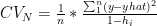
 is the diagonal hat matrix


 <
<  then have bowler ‘i’ to bowl more overs as his/her economy rate is better
 <
<  where the jth bowler is more effective than the kth bowler against the ith batsman. This now becomes a linear optimization problem as we can have several combinations of number of overs x economy rate for different bowlers and we will have to solve this algorithmically to determine the lowest score for bowling performance or highest score for batting order.


 then the question is
 and the total number of overs remaining to be bowled is N then –
 Also
Also 
