Identifying cricketing shots using AI

Image classification using Deep Learning has been around for almost a decade. In fact, this field with the use of Convolutional Neural Networks (CNN) is quite mature and the algorithms work very well in image classification, object detection, facial recognition and self-driving cars. In this post, I use AI image classification to identify cricketing shots. While the problem falls in a well known domain, the application of image  classification in identifying cricketing shots is probably new. I have selected three cricketing shots, namely, the front drive, sweep shot, and the hook shot for this purpose. My purpose was to build a proof-of-concept and not a perfect product. I have kept the dataset deliberately small (for obvious reasons) of just about 14 samples for each cricketing shot, and for a total of about 41 total samples for both training and test data. Anyway, I get a reasonable performance from the AI model.

Included below are some examples of the data set

This post is based on this or on Image classification from Hugging face. Interestingly, this, the model used here is based on Vision Transformers (ViT from Google Brain) and not on Convolutional Neural Networks as is usually done.

The steps are to fine-tune ViT Transformer with the ‘strokes’ dataset are

  1. Install the necessary libraries
! pip install transformers[torch] datasets evaluate accelerate -U
! pip install -U accelerate
! pip install -U transformers

b) Login to Hugging Face account

 from huggingface_hub import notebook_login
notebook_login()

Login successful

c) Load the batting strokes dataset with 41 images

from datasets import load_dataset
df1 = load_dataset("tvganesh/strokes",split='train')
type(df1)
len(df1)

41
df1
Dataset({
    features: ['image', 'label'],
    num_rows: 41
})

d) Create a dictionary that maps the label name to an integer and vice versa. Display the labels

labels = df1.features["label"].names
label2id, id2label = dict(), dict()
for i, label in enumerate(labels):
label2id[label] = str(i)
id2label[str(i)] = label

labels

['front drive', 'hook shot', 'sweep shot']

e) Load ViT image processor. To apply the correct transformations, ImageProcessor is initialised with a configuration that was saved along with the pretrained model 

from transformers import AutoImageProcessor

checkpoint = "google/vit-base-patch16-224-in21k"
image_processor = AutoImageProcessor.from_pretrained(checkpoint)

f) Apply image transformations to the images to make the model more robust against overfitting

from torchvision.transforms import RandomResizedCrop, Compose, Normalize, ToTensor

normalize = Normalize(mean=image_processor.image_mean, std=image_processor.image_std)
size = (
    image_processor.size["shortest_edge"]
    if "shortest_edge" in image_processor.size
    else (image_processor.size["height"], image_processor.size["width"])
)
_transforms = Compose([RandomResizedCrop(size), ToTensor(), normalize])

g) Create a preprocessing function to apply the transforms and return pixel_values of the image as the inputs to the model – :

def transforms(examples):
    examples["pixel_values"] = [_transforms(img.convert("RGB")) for img in examples["image"]]
    del examples["image"]
    return examples

h) Apply the preprocessing function over the entire dataset, using Hugging Face Dataset’s ‘with_transform’ method

df1 = df1.with_transform(transforms)
from transformers import DefaultDataCollator
data_collator = DefaultDataCollator()

i) Evaluate model’s performance with evaluate

import evaluate
accuracy = evaluate.load("accuracy")

j) Calculate accuracy by passing in predictions and labels

import numpy as np
def compute_metrics(eval_pred):
    predictions, labels = eval_pred
    predictions = np.argmax(predictions, axis=1)
    return accuracy.compute(predictions=predictions, references=labels)

k) Load ViT by specifying the number of labels along with the number of expected labels, and the label mapping

 from transformers import AutoModelForImageClassification, TrainingArguments, Trainer

model = AutoModelForImageClassification.from_pretrained(
    checkpoint,
    num_labels=len(labels),
    id2label=id2label,
    label2id=label2id,
)

l)

  1. Pass the training arguments to Trainer along with the model, dataset, tokenizer, data collator, and compute_metrics function.
  2. Call train() to finetune your model.
training_args = TrainingArguments(
    output_dir="data_classify",
    remove_unused_columns=False,
    evaluation_strategy="epoch",
    save_strategy="epoch",
    learning_rate=5e-5,
    per_device_train_batch_size=8,
    #gradient_accumulation_steps=4,
    per_device_eval_batch_size=6,
    num_train_epochs=20,
    warmup_ratio=0.1,
    logging_steps=10,
    load_best_model_at_end=True,
    metric_for_best_model="accuracy",
    push_to_hub=True,
)

trainer = Trainer(
    model=model,
    args=training_args,
    data_collator=data_collator,
    train_dataset=train_dataset,
    eval_dataset=test_dataset,
    tokenizer=image_processor,
    compute_metrics=compute_metrics,
)

trainer.train()

Epoch	Training Loss	Validation Loss	Accuracy
1	No log	0.434451	1.000000
2	No log	0.388312	1.000000
3	0.361200	0.409932	0.888889
4	0.361200	0.245226	1.000000
5	0.293400	0.196930	1.000000
6	0.293400	0.167858	1.000000
7	0.293400	0.140349	1.000000
8	0.203000	0.153016	1.000000
9	0.203000	0.116115	1.000000
10	0.150500	0.129171	1.000000
11	0.150500	0.103121	1.000000
12	0.150500	0.108433	1.000000
13	0.138800	0.107799	1.000000
14	0.138800	0.093700	1.000000
15	0.107600	0.100769	1.000000
16	0.107600	0.113148	1.000000
17	0.107600	0.100740	1.000000
18	0.104700	0.177483	0.888889
19	0.104700	0.084438	1.000000
20	0.090200	0.112654	1.000000
TrainOutput(global_step=80, training_loss=0.18118578270077706, metrics={'train_runtime': 176.3834, 'train_samples_per_second': 3.628, 'train_steps_per_second': 0.454, 'total_flos': 4.959531785650176e+16, 'train_loss': 0.18118578270077706, 'epoch': 20.0})

m) Push to Hub

trainer.push_to_hub()

You can try out my fine-tuned model at identify_stroke̱

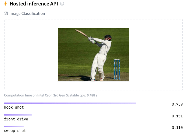
Here are a couple of trials
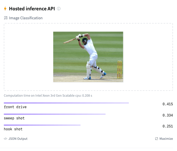
As I mentioned before, the model should be reasonably accurate but not perfect, since my training dataset is extremely small. This is just a prototype to show that shot identification in cricket with AI is in the realm of the possible.

References

  1. Image classification
  2. AN IMAGE IS WORTH 16X16 WORDS:TRANSFORMERS FOR IMAGE RECOGNITION AT SCALE

Do take a look at

  1. Using Reinforcement Learning to solve Gridworld
  2. Deconstructing Convolutional Neural Networks with Tensorflow and Keras
  3. GenerativeAI:Using T5 Transformer model to summarise Indian Philosophy
  4. GooglyPlusPlus: Win Probability using Deep Learning and player embeddings
  5. T20 Win Probability using CTGANs, synthetic data
  6. Deep Learning from first principles in Python, R and Octave – Part 6
  7. Introducing QCSimulator: A 5-qubit quantum computing simulator in R
  8. Big Data 6: The T20 Dance of Apache NiFi and yorkpy
  9. Re-introducing cricketr! : An R package to analyze performances of cricketers

To see all posts click Index of posts

GenerativeAI:Using T5 Transformer model to summarise Indian Philosophy

Ever since I started to use ChatGPT,  I have been fascinated by its capabilities. To a large extent, the abilities of  Large  Language Models (LLMs) is quite magical – the way it answers questions, the way it summarises passages, the way it creates  poems et cetera. All the LLMs need is a large corpus of data from the internet, articles, wikis, blogs, and so on.

On delving a little deeper into Generative AI, LLMs I learnt that, this is based on the principle of being able to predict the most probable word in a given sequence. It made me wonder whether the world of ideas, language and communication are actually governed by probabilities. Does what we communicate fall within the purview of statistics?

As an aside, just by extending further if we visualise a world in which  every human action to a situation is assigned an embedding vector, and if we feed the responses of all humans over time in  different situations, to the equivalent of a Transformer of a Large Human Reaction Model (LHRM) ;-),  we can envisage the model being capable of predicting the response of human in a given situation. In my opinion, the machine would be fairly right most of the occasions as it could select the most probable choice of action, much like ‘The Machine’ in Person of Interest. However, this does not mean that the machine (AI) is actually more intelligent than humans. All it means is that the choice of humans responses are a part of a finite subset possibilities and The Machine (AI) can compute the possibilities and associated probabilities much quicker than humans. Does it mean that the world is deterministic? Possibly.

In this post, I use the T5 transformer to summarise Indian philosophy. For this task, I have fine-tuned the T5 model with a curated dataset taken from random passages on Hindu philosophy available on the internet. For each passage, I had to and hand-create the corresponding summary. This was a fairly tedious and demanding task but an enlightening one. It was interesting to understand how our ancestors, the Rishis, understood reality, the physical world, senses, the mind, the intellect, consciousness (Atman) and universal consciousness (Brahman). (Incidentally I was only able to curate only about 130 rows of philosophical snippets and manually create the corresponding summaries. Probably this is a very small dataset for fine-tuning but I just wanted to see the performance of the T5 model in a new domain.)

In this post the T5 model is fine-tuned with the curated dataset and the rouge1 and rouge2 scores are used to evaluate the model’s performance.

I have used the Hugging Face Hub for the transformer model, corresponding LLM functions and management of the dataset etc. The Hugging Face ecosystem is simply wow!!

Summarisation with T5-small model

a) Install the necessary libraries

! pip install transformers[torch] datasets evaluate rouge_score accelerate -U
! pip install -U accelerate
! pip install -U transformers

b) Login to Hugging Face account


from huggingface_hub import notebook_login
notebook_login()

Login successful

c) Load the curated dataset on Hindu philosophy

from datasets import load_dataset
df1 = load_dataset("tvganesh/philosophy",split='train')

d) Load a T5 tokenizer to process text and summary

  1. Prefix the input with a prompt so T5 knows this is a summarization task.
  2. Use the keyword text_target argument when tokenizing labels.
  3. Truncate sequences to be no longer than the maximum length set by the max_length parameter. The max_length of the text kept at 220 words and the max_length  of the summary is kept at 50 words.
  4. The ‘map’ function of the Huggingface dataset can be used to apply the pre_process function across the entire data.
from transformers import AutoTokenizer

checkpoint = "t5-small"
#checkpoint = "facebook/bart-large-cnn"
tokenizer = AutoTokenizer.from_pretrained(checkpoint)

prefix = "summarize: "

def preprocess_function(passages):
    inputs = [prefix + doc for doc in passages["text"]]
    model_inputs = tokenizer(inputs, max_length=220, truncation=True)

    labels = tokenizer(text_target=passages["summary"], max_length=50, truncation=True)

    model_inputs["labels"] = labels["input_ids"]
    return model_inputs

tokenized_df1 = df1.map(preprocess_function, batched=True)

DataCollatorForSeq2Seq can be used to dynamically pad the sentences to the longest length in a batch during collation, instead of padding the whole dataset to the maximum length.

from transformers import DataCollatorForSeq2Seq
data_collator = DataCollatorForSeq2Seq(tokenizer=tokenizer, model=checkpoint)

e) Evaluate performance of Model

The rouge1,rouge2  metric can be used to evaluate the performance of the model

import evaluate
rouge = evaluate.load("rouge")

f)Create a function compute_metrics that passes your predictions and labels to ‘compute’ to calculate the ROUGE metric:

import numpy as np

def compute_metrics(eval_pred):
    # evaluate predictions and labels
    predictions, labels = eval_pred
    decoded_preds = tokenizer.batch_decode(predictions, skip_special_tokens=True)
    labels = np.where(labels != -100, labels, tokenizer.pad_token_id)
    decoded_labels = tokenizer.batch_decode(labels, skip_special_tokens=True)
     # compute rouge score between the labels and predictions
    result = rouge.compute(predictions=decoded_preds, references=decoded_labels, use_stemmer=True)

    prediction_lens = [np.count_nonzero(pred != tokenizer.pad_token_id) for pred in predictions]
    result["gen_len"] = np.mean(prediction_lens)

    return {k: round(v, 4) for k, v in result.items()}

g) Split the data into training(80%)  and test(20%) data set

train_dataset = tokenized_df1.shuffle(seed=42).select(range(100))
test_dataset = tokenized_df1.shuffle(seed=42).select(range(30))

len(train_dataset)

h) Train the model with AutoModelForSeq2SeqLM

from transformers import AutoModelForSeq2SeqLM, Seq2SeqTrainingArguments, Seq2SeqTrainer
model = AutoModelForSeq2SeqLM.from_pretrained(checkpoint)

i)

  1. Set training hyperparameters in Seq2SeqTrainingArguments. The Adam optimization, with learning rate, beta1 & beta2 are used
  2. Pass the training arguments to Seq2SeqTrainer along with the model, dataset, tokenizer, data collator, and compute_metrics function.
  3. Call train() to finetune your model.
training_args = Seq2SeqTrainingArguments(
    output_dir="philosophy_model",
    evaluation_strategy="epoch",
    learning_rate= 5.6e-03,
    adam_beta1=0.9,
    adam_beta2=0.99,
    adam_epsilon=1e-06,
    per_device_train_batch_size=8,
    per_device_eval_batch_size=8,
    weight_decay=0.01,
    save_total_limit=3,
    num_train_epochs=20,
    predict_with_generate=True,
    fp16=True,
    push_to_hub=True,
)

trainer = Seq2SeqTrainer(
    model=model,
    args=training_args,
    train_dataset=train_dataset,
    eval_dataset=test_dataset,
    tokenizer=tokenizer,
    data_collator=data_collator,
    compute_metrics=compute_metrics,
)

trainer.train()

Epoch	Training Loss	Validation Loss	Rouge1	Rouge2	Rougel	Rougelsum	Gen Len
1	No log	2.246223	0.363200	0.146200	0.311400	0.312600	18.333300
2	No log	1.461140	0.459000	0.303900	0.417800	0.417800	18.566700
3	No log	0.832312	0.546500	0.425900	0.524700	0.520800	17.133300
4	No log	0.472341	0.616100	0.517600	0.601000	0.600400	18.366700
5	No log	0.312106	0.681200	0.607800	0.674700	0.671400	18.233300
6	No log	0.154585	0.741800	0.702300	0.733800	0.731300	18.066700
7	No log	0.112100	0.783200	0.763000	0.780200	0.778900	18.500000
8	No log	0.069882	0.801400	0.788200	0.802700	0.800900	18.533300
9	No log	0.045941	0.795800	0.780500	0.794600	0.791700	18.500000
10	No log	0.051655	0.809100	0.795800	0.810500	0.809000	18.466700
11	No log	0.035792	0.799400	0.785200	0.797300	0.794600	18.500000
12	No log	0.041766	0.779900	0.754800	0.774700	0.773200	18.266700
13	No log	0.010703	0.810000	0.800400	0.810700	0.809000	18.500000
14	No log	0.006519	0.807700	0.797100	0.809400	0.807500	18.500000
15	No log	0.017779	0.808000	0.796000	0.809400	0.807500	18.366700
16	No log	0.001681	0.810000	0.800400	0.810700	0.809000	18.500000
17	No log	0.005469	0.810000	0.800400	0.810700	0.809000	18.500000
18	No log	0.002003	0.810000	0.800400	0.810700	0.809000	18.500000
19	No log	0.000638	0.810000	0.800400	0.810700	0.809000	18.500000
20	No log	0.000498	0.810000	0.800400	0.810700	0.809000	18.500000
TrainOutput(global_step=260, training_loss=0.6491916949932391, metrics={'train_runtime': 57.99, 'train_samples_per_second': 34.489, 'train_steps_per_second': 4.484, 'total_flos': 101132046434304.0, 'train_loss': 0.6491916949932391, 'epoch': 20.0})

As we can see the rouge1 to rouge2 scores are fairly good. Anything above 0.5 is considered good. Maybe this is because the T5 model has already been pre-trained on a fairly large philosophical dataset

j) Push to hub

trainer.push_to_hub()

k) Summarise using pipeline

text = "summarize: A seeker who has the necessary qualifications, in order that he may be redeemed from his inner weaknesses, attachments, animalisms and false values is advised to serve with devotion a Teacher who is well- established in the experience of the Self."

from transformers import pipeline

summarizer = pipeline("summarization", model="tvganesh/philosophy_model")
summarizer(text)

[{'summary_text': 'A seeker who has the necessary qualifications will be able to free oneself of sense objects, and one cannot expect this to happen without any mental tossing'}]

l) Summarise using model generate

from transformers import AutoTokenizer

tokenizer = AutoTokenizer.from_pretrained("tvganesh/philosophy_model")
inputs = tokenizer(text, return_tensors="pt").input_ids

from transformers import AutoModelForSeq2SeqLM

model = AutoModelForSeq2SeqLM.from_pretrained("tvganesh/philosophy_model")
outputs = model.generate(inputs, max_new_tokens=70, do_sample=False)

tokenizer.decode(outputs[0], skip_special_tokens=True)

'A seeker who has the necessary qualifications will help in his journey to redeem himself'

l) Number of beams

summary_ids = model.generate(inputs,
                                    num_beams=10,
                                    no_repeat_ngram_size=3,
                                    min_length=20,
                                    max_length=70,
                                    early_stopping=True)
output = tokenizer.decode(summary_ids[0], skip_special_tokens=True)
output

'A seeker who has the necessary qualifications will be able to free himself of sense objects and false values'

I also tried Facebook’s BART Large model but the performance was not good at all.

You can try out the model at the following link philosophy_model

Anyway this was a good learning experience.

References

  1. Summarisation
  2. Fine-tune a pre-trained model
  3. Generative AI with Large Language Models , Coursera

Also see

  1. Deep Learning from first principles in Python, R and Octave – Part 4
  2. Introducing QCSimulator: A 5-qubit quantum computing simulator in R
  3. Computing IPL player similarity using Embeddings, Deep Learning
  4. Natural language processing: What would Shakespeare say?
  5. Using Linear Programming (LP) for optimizing bowling change or batting lineup in T20 cricket
  6. Revisiting World Bank data analysis with WDI and gVisMotionChart
  7. Big Data-4: Webserver log analysis with RDDs, Pyspark, SparkR and SparklyR
  8. Sea shells on the seashore
  9. Experiments with deblurring using OpenCV
  10. A closer look at “Robot Horse on a Trot” in Android

To see all posts click Index of posts