What would you think if I sang out of tune? Would you stand up and walk out on me? Lend me your ears and I’ll sing you a song And I’ll try not to sing out of key
Oh, I get by with a little help from AI Mm, I get high with a little help from AI Mm, gonna try with a little help with AI
Adapted from “With A Little Help From My Friends” from the album Sgt. Pepper’s Lonely Heart Club Band, Beatles, 1967
Introduction For quite some time I have been wanting to create an application that allows user to query cricket data in plain English (Natural Language Query) and get the appropriate answer. Finally, I have been able to realise this idea with my latest application “IPL AI Oracle:AI that speaks cricket!!!“. While I have just done this for IPL, it can be done for any of the other T20 leagues namely (Intl. T20 Men’s and Women’s, BBL, PSL, NTB, CPL, WBBL etc.). The current app “IPL AI Oracle” is in Python, and is a distant cousin of my Shiny app GooglyPlusPlus written entirely in R (see IPL 2023:GooglyPlusPlus now with by AI/ML models, near real-time analytics!)
GooglyPlusPlus is much more sophisticated with detailed analytics of batsmen, bowlers, teams, matches, head-to-head, team-vs-AllTeams, batsmen and bowler ranking and analyis. GooglyPlus also includes ball-by-ball Win Probability models using Logistic Regression and Deep Learning models. While, ‘IPL AI Oracle’ lacks the ML/DL models it includes the ability to answer user queries in simple English (Natural Language Query -NLQ) and generate the pandas code for the same.
IPL AI Oracle
The IPL AI Oracle has a 2 main modules
frontend
backend
a) Frontend
The frontend is made with Next.js, Typescript and has 4 tabs
General queries
Match Analysis
Head-to-head
Team vs All Teams
The frontend includes analytics for matches, head-to-head and team-vs-allTeams options. Plots can be generated for some features and uses Plotly.js for rendering of plots
b) Backend
The backend implements FastAPI endpoints for the different analytics and natural language queries. A) The analytics in the 3 tabs namely match analysis, head-to-head and team vs All teams are implemented using my Python package ‘yorkpy‘. Since my package yorkpy has all the cricket rules baked into it, I used the code from my package verbatim for these tabs.
B) The data for the analytics comes from Cricsheet. Cricsheet includes ball-by-ball data in yaml, for all IPL matches from the beginning of time. This data is pre-processed with R utilities of my Shiny app GooglyPlusPlus. These R functions to convert the match data into the data required format for the a) Match Analysis Tab b) Head-to-head tab and c) Team vs All Teams tab which are then subsequently converted to csv for use by my package yorkpy. My Python package is based on pandas and can process this data and display the analytics required for the tabs
C) Plotly is used for generating the plots
D) Jinja templates are used for creating the prompts for the different tabs
D) For natural language query in each tab, originally I used Ollama and tried out Mistral 7Band DeepSeek Coder 6.7B. But then I realised that it has a large footprint, if deployed, and hence settled for gpt-4.1-nano
The frontend is deployed on Vercel and the backend is dockerised and deployed on Railway. Since the clock is ticking for Vercel, Railway and GPT API, I will be closely monitoring the usage.
Give IPL AI Oracle a try. Click this link IPL AI Oracle. (When you click the link you will be asked to enter your email address, to which a magic link will be sent. Clicking the link will give access to the link. Please wait 2-3 minutes for the mail, if still not received check your spam/trash folder)
Here are some random screenshots from the different tabs
I) IPL Analytics A) Match Analysis a) Batting scorecard – Chennai Super Kings vs Gujarat Titans (2025-05-25)
b) Batsmen vs Bowlers (Mumbai Indians vs Delhi Capitals – 2025-04-13)
B) Head-to-head Analysis
a) Top Bowlers Performance (Delhi Capitals vs Kolkata Knight Riders – all matches) This tab takes into consideration all matches played between these 2 teams and computes analytics between these 2 teams
b) Wicket Types Analysis (Rajasthan Royals vs Mumbai Indians – all matches)
C) Team vs All Teams
a) Team Bowling Scorecard – Royal Challengers Bangalore
II) Natural Language Query (User queries)
A) General Queries i) How many runs did V Kohli score in total ?
ii) How runs did MS Dhoni score in 2017?
iii) Which team won the most matches?
iv) Which bowler has the best economy rate?
v) How many times did Chennai Super Kings defeat Rajasthan Royals?
vi) How many wickets did Bumrah take in 2017?
B) Match analysis – Natural Language query
To use the Natural Language Query in this tab, you have to choose the match. For e.g.Chennai Super Kings vs Mumbai Indians (2025-04-20). Selecting a match between 2 teams will automatically create natural language chips (with red arrow). You can select any one of the chips (button) or type in your own question and click Ask Question
i) Who scored the most runs in this match?
This can be verified by selecting the Batting scorecard for the match
ii) Who took the most wickets in this match?
iii) What is the economy rate of JC Archer?
C) Head-vs-Head (Natural Language Query)
Before typing in a Natural Language Query (NLQ) ensure that Team 1 and Team 2 are selected
a) Which bowler took the most wickets between Royal Challengers Bangalore and Chennai Super Kings?
b) Which batsmen scored between 30 to 40 runs in these matches?
D) Team vs All Teams (Natural Language Query)
Remember to select the Team before using NLQ
a) Who are the top 3 batsman for Gujarat Titans?
b) What was Punjab King’s win percentage?
How I Built IPL AI Oracle (with a Little Help from AI)
Here are key highlights behind the build
Data for this app comes from Cricsheet which provides ball-by-ball details in every IPL match as yaml files
Pre-processing of these yaml files were done using R utilities I already had into RData data frames, which were then subsequently converted to CSV for the different tabs
All the analytics is based on my handcoded package yorkpy as it has all the cricket rules baked in
AI assisted coding was used quite heavily for the front-end and the FastAPI backend. This was done using Cursor either with Sonnet 4.5 or GPT-5 Codex
Prompt templates for the different tabs were hand-crafted based on my package yorkpy
All-in all, the application is a healthy mix of hand-coding and AI assisted coding.
Conclusion
Since I had to deploy the application in 3 different platforms a) Vercel b) Railway c) OpenAI. I have the clock ticking in all these platforms. I initially tried gpt-4.1-mini (SLM) and then switched to gpt-4.1-nano (Tiny LM) as it is more cost effective. Since the gpt-4.1-nano has only a few hundred million parameters and is designed for low latency and cost-effectiveness, it is not as forgiving to typos or incorrect names, as some of the bigger LLMs like GPT-4o or Sonnet 4.5. Hence natural language queries work in most situations but at times they do fail. It requires quite a bit of fine-tuning I guess. Maybe work for some other day, by which time I hope the $X =N tokens/million come down drastically, so that even hobbyists like me can afford it comfortably.
Do check out IPL AI Oracle! You will get a magic link which will enable access.
In this post, I compute each batsman’s or bowler’s Win Probability Contribution (WPC) in a T20 match. This metric captures by how much the player (batsman or bowler) changed/impacted the Win Probability of the T20 match. For this computation I use my machine learning models, I had created earlier, which predicts the ball-by-ball win probability as the T20 match progresses through the 2 innings of the match.
In the picture snippet below, you can see how the win probability changes ball-by-ball for each batsman for a T20 match between CSK vs LSG- 31 Mar 2022
In my previous posts I had created several Machine Learning models. In order to compute the player’s Win Probability contribution in this post, I have used the following ML models
The batsman’s or bowler’s win probability contribution changes ball-by=ball. The player’s contribution is calculated as the difference in win probability when the batsman faces the 1st ball in his innings and the last ball either when is out or the innings comes to an end. If the difference is +ve the the player has had a positive impact, and likewise for negative contribution. Similarly, for a bowler, it is the win probability when he/she comes into bowl till, the last delivery he/she bowls
Note: The Win Probability Contribution does not have any relation to the how much runs or at what strike rate the batsman scored the runs. Rather the model computes different win probability for each player, based on his/her embedding, the ball in the innings and six other feature vectors like runs, run rate, runsMomentum etc. These values change for every ball as seen in the table above. Also, this is not continuous. The 2 ML models determine the Win Probability for a specific player, ball and the context in the match.
This metric is similar to Win Probability Added (WPA) used in Sabermetrics for baseball. Here is the definition of WPA from Fangraphs “Win Probability Added (WPA) captures the change in Win Expectancy from one plate appearance to the next and credits or debits the player based on how much their action increased their team’s odds of winning.” This article in Fangraphs explains in detail how this computation is done.
In this post I have added 4 new function to my R package yorkr.
batsmanWinProbLR – batsman’s win probability contribution based on glmnet (Logistic Regression)
bowlerWinProbLR – bowler’s win probability contribution based on glmnet (Logistic Regression)
batsmanWinProbDL – batsman’s win probability contribution based on Deep Learning Model
bowlerWinProbDL – bowlerWinProbLR – bowler’s win probability contribution based on Deep Learning
Hence there are 4 additional features in GooglyPlusPlus based on the above 4 functions. In addition I have also updated
-winProbLR (overLap) function to include the names of batsman when they come to bat and when they get out or the innings comes to an end, based on Logistic Regression
-winProbDL(overLap) function to include the names of batsman when they come to bat and when they get out based on Deep Learning
Hence there are 6 new features in this version of GooglyPlusPlus.
Note: All these new 6 features are available for all 9 formats of T20 in GooglyPlusPlus namely
a) IPL b) BBL c) NTB d) PSL e) Intl, T20 (men) f) Intl. T20 (women) g) WBB h) CSL i) SSM
Check out the latest version of GooglyPlusPlus at gpp2023-2
Note: The data for GooglyPlusPlus comes from Cricsheet and the Shiny app is based on my R package yorkr
A) Chennai SuperKings vs Delhi Capitals – 04 Oct 2021
To understand Win Probability Contribution better let us look at Chennai Super Kings vs Delhi Capitals match on 04 Oct 2021
This was closely fought match with fortunes swinging wildly. If we take a look at the Worm wicket chart of this match
a) Worm Wicket chart – CSK vs DC – 04 Oct 2021
Delhi Capitals finally win the match
b) Win Probability Logistic Regression (side-by-side) – CSK vs DC – 4 Oct 2021
Plotting how win probability changes over the course of the match using Logistic Regression Model
In this match Delhi Capitals won. The batting scorecard of Delhi Capitals
c) Batting Scorecard of Delhi Capitals – CSK vs DC – 4 Oct 2021
d) Win Probability Logistic Regression (Overlapping) – CSK vs DC – 4 Oct 2021
The Win Probability LR (overlapping) shows the probability function of both teams superimposed over one another. The plot includes when a batsman came into to play and when he got out. This is for both teams. This looks a little noisy, but there is a way to selectively display the change in Win Probability for each team. This can be done , by clicking the 3 arrows (orange or blue) from top to bottom. First double-click the team CSK or DC, then click the next 2 items (blue,red or black,grey) Sorry the legends don’t match the colors! 🙁
Below we can see how the win probability changed for Delhi Capitals during their innings, as batsmen came into to play. See below
e)Batsman Win Probability contribution:DC – CSK vs DC – 4 Oct 2021
Computing the individual batsman’s Win Contribution and plotting we have. Hetmeyer has a higher Win Probability contribution than Shikhar Dhawan depsite scoring fewer runs
f) Bowler’s Win Probability contribution :CSK – CSK vs DC – 4 Oct 2021
We can also check the Win Probability of the bowlers. So for e.g the CSK bowlers and which bowlers had the most impact. Moeen Ali has the least impact in this match
B) Intl. T20 (men) Australia vs India – 25 Sep 2022
a) Worm wicket chart – Australia vs India – 25 Sep 2022
This was another close match in which India won with the penultimate ball
b) Win Probability based on Deep Learning model (side-by-side) –Australia vs India – 25 Sep 2022
c) Win Probability based on Deep Learning model (overlapping) –Australia vs India – 25 Sep 2022
The plot below shows how the Win Probability of the teams varied across the 20 overs. The 2 Win Probability distributions are superimposed over each other
d) Batsman Win Probability Contribution : India – Australia vs India – 25 Sep 2022
Selectively choosing the India Win Probability plot by double-clicking legend ‘India’ on the right , followed by single click of black, grey legend we have
We see that Kohli, Suryakumar Yadav have good contribution to the Win Probability
e) Plotting the Runs vs Strike Rate:India – Australia vs India – 25 Sep 2022
f) Batsman’s Win Probability Contribution-Australia vs India – 25 Sep 2022
Finally plotting the Batsman’s Win Probability Contribution
Interestingly, Kohli has a greater Win Probability Contribution than SKY, though SKY scored more runs at a better strike rate. As mentioned above, the Win Probability is context dependent and also depends on past performances of the player (batsman, bowler)
Finally let us look at
C) India vs England Intll T20 Women (11 July 2021)
a) Worm wicket chart – India vs England Intl. T20 Women (11 July 2021)
India won this T20 match by 8 runs
b) Win Probability using the Logistic Regression Model –India vs England Intl. T20 Women (11 July 2021)
c) Win Probability with the DL model –India vs England Intl. T20 Women (11 July 2021)
d) Bowler Win Probability Contribution with the LR model–India vs England Intl. T20 Women (11 July 2021)
e) Bowler Win Contribution with the DL model–India vs England Intl. T20 Women (11 July 2021)
Go ahead and try out the latest version of GooglyPlusPlus
In my last post ‘GooglyPlusPlus now with Win Probability Analysis for all T20 matches‘ I had discussed the performance of my ML models, created with and without player embeddings, in computing the Win Probability of T20 matches. With batsman & bowler embeddings I got much better performance than without the embeddings
glmnet – Accuracy – 0.73
Random Forest (RF) – Accuracy – 0.92
While the Random Forest gave excellent accuracy, it was bulky and also took an unusually long time to predict the Win Probability of a single T20 match. The above 2 ML models were built using R’s Tidymodels. glmnet was fast, but I wanted to see if I could create a ML model that was better, lighter and faster. I had initially tried to use Tensorflow, Keras in Python but then abandoned it, since I did not know how to port the Deep Learning model to R and use in my app GooglyPlusPlus.
But later, since I was stuck with a bulky Random Forest model, I decided to again explore options for saving the Keras Deep Learning model and loading it in R. I found out that saving the model as .h5, we can load it in R and use it for predictions. Hence, I rebuilt a Deep Learning model using Keras, Python with player embeddings and I got excellent performance. The DL model was light and had an accuracy 0.8639 with an ROC_AUC of 0.964 which was great!
GooglyPlusPlus uses data from Cricsheet and is based on my R package yorkr
You can try out this latest version of GooglyPlusPlus at gpp2023-1
Here are the steps
A. Build a Keras Deep Learning model
a. Import necessary packages
import pandas as pd
import numpy as np
from zipfile import ZipFile
import tensorflow as tf
from tensorflow import keras
from tensorflow.keras import layers
from tensorflow.keras import regularizers
from pathlib import Path
import matplotlib.pyplot as plt
b, Upload the data of all 9 T20 leagues (BBL, CPL, IPL, T20 (men) , T20(women), NTB, CPL, SSM, WBB)
# Read all T20 leagues
df1=pd.read_csv('t20.csv')
print("Shape of dataframe=",df1.shape)

# Create training and test data set
train_dataset = df1.sample(frac=0.8,random_state=0)
test_dataset = df1.drop(train_dataset.index)
train_dataset1 = train_dataset[['batsmanIdx','bowlerIdx','ballNum','ballsRemaining','runs','runRate','numWickets','runsMomentum','perfIndex']]
test_dataset1 = test_dataset[['batsmanIdx','bowlerIdx','ballNum','ballsRemaining','runs','runRate','numWickets','runsMomentum','perfIndex']]
train_dataset1

# Set the target data
train_labels = train_dataset.pop('isWinner')
test_labels = test_dataset.pop('isWinner')
train_dataset1

a=train_dataset1.describe()
stats=a.transpose
a
c. Create a Deep Learning ML model using batsman & bowler embeddings
This was a huge success for me to be able to create the Deep Learning model in Python and use it in my Shiny app GooglyPlusPlus. The Deep Learning Keras model is light-weight and extremely fast.
The Deep Learning model has now been integrated into GooglyPlusPlus. Now you can check the Win Probability using both a) glmnet (Logistic Regression with lasso regularisation) b) Keras Deep Learning model with dropouts as regularisation
In addition I have created 2 features based on Win Probability (WP)
i) Win Probability (Side-by-side– Plot(interactive) : With this functionality the 1st and 2nd innings will be side-by-side. When the 1st innings is played by team 1, the Win Probability of team 2 = 100 – WP (team1). Similarly, when the 2nd innings is being played by team 2, the Win Probability of team1 = 100 – WP (team 2)
ii) Win Probability (Overlapping) – Plot (static): With this functionality the Win Probabilities of both team1(1st innings) & team 2 (2nd innings) are displayed overlapping, so that we can see how the probabilities vary ball-by-ball.
Note: Since the same UI is used for all match functions I had to re-use the Plot(interactive) and Plot(static) radio buttons for Win Probability (Side-by-side) and Win Probability(Overlapping) respectively
Here are screenshots using both ML models with both functionality for some random matches
B) ICC T20 Men World Cup – Netherland-South Africa- 2022-11-06
i) Match Worm wicket chart
ii) Win Probability with LR (Side-by-Side- Plot(interactive))
iii) Win Probability LR (Overlapping- Plot(static))
iv) Win Probability Deep Learning (Side-by-side – Plot(interactive)
In the 213th ball of the innings South Africa was slightly ahead of Netherlands. After that they crashed and burned!
v) Win Probability Deep Learning (Overlapping – Plot (static)
It can be seen that in the 94th ball of both innings South Africa was ahead of Netherlands before the eventual slump.
C) Intl. T20 (Women) India – New Zealand – 2020 – 02 – 27
Here is an interesting match between India and New Zealand T20 Women’s teams. NZ successfully chased the India’s total in a wildly swinging fortunes. See the charts below
i) Match Worm Wicket chart
ii) Win Probability with LR (Side-by-side – Plot (interactive)
iii) Win Probability with LR (Overlapping – Plot (static)
iv) Win Probability with DL model (Side-by-side – Plot (interactive))
v) Win Probability with DL model (Overlapping – Plot (static))
The above functionality in plotting the Win Probability using LR or DL with both options (Side-by-side or Overlapping) is available for all 9 T20 leagues currently supported by GooglyPlusPlus.
In my previous post Computing Win Probability of T20 matches I had discussed various approaches on computing Win Probability of T20 matches. I had created ML models with glmnet and random forest using TidyModels. This was what I had achieved
glmnet : accuracy – 0.67 and sensitivity/specificity – 0.68/0.65
random forest : accuracy – 0.737 and roc_auc- 0.834
DL model with Keras in Python : accuracy – 0.73
I wanted to see if the performance of the models could be further improved. I got a suggestion from a AI/DL whizkid, who is close to me, to include embeddings for batsmen and bowlers. He felt that win percentage is influenced by which batsman faces which bowler.
So, I started to explore this idea. Embeddings can be used to convert categorical variables to a vector of continuous floating point numbers.Fortunately R’s Tidymodels, has a convenient functionality to create embeddings. By including embeddings for batsman, bowler the performance of my ML models improved vastly. Now the performance is
glmnet : accuracy – 0.728 and roc_auc – 0.81
random forest : accuracy – 0.927 and roc_auc – 0.98
mlp-dnn :accuracy – 0.762 and roc_auc – 0.854
As can be seem there is almost a 20% increase in accuracy with random forests with embeddings over the model without embeddings. Moreover, the feature importance which is plotted below shows that the bowler and batsman embeddings have a significant influence on the Win Probability
Note: The data for this analysis is taken from Cricsheet and has been processed with my R package yorkr.
A. Win Probability using GLM with penalty and player embeddings
Here Generalised Linear Model (GLMNET) for Logistic Regression is used. In the GLMNET the regularisation path is computed for the lasso or elastic net penalty at a grid of values for the regularisation parameter lambda. glmnet is extremely fast and gave an accuracy of 0.72 for an roc_auc of 0.81 with batsman, bowler embeddings. This was good improvement over my earlier implementation with glmnet without the batsman & bowler embeddings which had a
Read the data
a) Read the data from 9 T20 leagues (BBL, CPL, IPL, NTB, PSL, SSM, T20 Men, T20 Women, WBB) and create a single data frame of ball-by-ball data. Display the data frame
b) Split to training, validation and test sets. The dataset is initially split into training and test in the ratio 80%:20%. The training data is again split into training and validation in the ratio 80:20
4) Create a Logistic Regression Workflow by adding the GLM model and the recipe
5) Create grid of elastic penalty values for regularisation
6) Train all 30 models
7) Plot the ROC of the model against the penalty
# Use all 12 cores
cores <- parallel::detectCores()
cores
# Create a Logistic Regression model with penalty
lr_mod <-
  logistic_reg(penalty = tune(), mixture = 1) %>%
  set_engine("glmnet",num.threads = cores)

# Create pre-processing recipe
lr_recipe <-
  recipe(isWinner ~ ., data = df_other) %>%
  step_embed(batsman,bowler, outcome = vars(isWinner)) %>%  step_normalize(ballNum,ballsRemaining,runs,runRate,numWickets,runsMomentum,perfIndex)

# Set the workflow by adding the GLM model with the recipe
lr_workflow <-
  workflow() %>%
  add_model(lr_mod) %>%
  add_recipe(lr_recipe)

# Create a grid for the elastic net penalty
lr_reg_grid <- tibble(penalty = 10^seq(-4, -1, length.out = 30))
lr_reg_grid %>% top_n(-5)
# A tibble: 5 × 1
   penalty

<dbl>
1 0.0001
2 0.000127
3 0.000161
4 0.000204
5 0.000259

lr_reg_grid %>% top_n(5)  # highest penalty values
# A tibble: 5 × 1
  penalty
    <dbl>
1  0.0386
2  0.0489
3  0.0621
4  0.0788
5  0.1

# Train 30 penalized models
lr_res <-
  lr_workflow %>%
  tune_grid(val_set,
            grid = lr_reg_grid,
            control = control_grid(save_pred = TRUE),
            metrics = metric_set(accuracy,roc_auc))

# Plot the penalty versus ROC
lr_plot <-
  lr_res %>%
  collect_metrics() %>%
  ggplot(aes(x = penalty, y = mean)) +
  geom_point() +
  geom_line() +
  ylab("Area under the ROC Curve") +
  scale_x_log10(labels = scales::label_number())

lr_plot
The Penalty vs ROC plot is shown below
8) Display the ROC_AUC of the top models with the penalty
9) Select the model with the best ROC_AUC and the associated penalty. It can be seen the best mean ROC_AUC is 0.81 and the associated penalty is 0.000530
top_models <-
  lr_res %>%
  show_best("roc_auc", n = 15) %>%
  arrange(penalty)
top_models

# A tibble: 15 × 7
    penalty .metric .estimator  mean     n std_err .config
      <dbl> <chr>   <chr>      <dbl> <int>   <dbl> <chr>
 1 0.0001   roc_auc binary     0.810     1      NA Preprocessor1_Model01
 2 0.000127 roc_auc binary     0.810     1      NA Preprocessor1_Model02
 3 0.000161 roc_auc binary     0.810     1      NA Preprocessor1_Model03
 4 0.000204 roc_auc binary     0.810     1      NA Preprocessor1_Model04
 5 0.000259 roc_auc binary     0.810     1      NA Preprocessor1_Model05
 6 0.000329 roc_auc binary     0.810     1      NA Preprocessor1_Model06
 7 0.000418 roc_auc binary     0.810     1      NA Preprocessor1_Model07
 8 0.000530 roc_auc binary     0.810     1      NA Preprocessor1_Model08
 9 0.000672 roc_auc binary     0.810     1      NA Preprocessor1_Model09
10 0.000853 roc_auc binary     0.810     1      NA Preprocessor1_Model10
11 0.00108  roc_auc binary     0.810     1      NA Preprocessor1_Model11
12 0.00137  roc_auc binary     0.810     1      NA Preprocessor1_Model12
13 0.00174  roc_auc binary     0.809     1      NA Preprocessor1_Model13
14 0.00221  roc_auc binary     0.809     1      NA Preprocessor1_Model14
15 0.00281  roc_auc binary     0.809     1      NA Preprocessor1_Model15

#Picking the best model and the corresponding penalty
lr_best <-
  lr_res %>%
  collect_metrics() %>%
  arrange(penalty) %>%
  slice(8)
lr_best
# A tibble: 1 × 7

   penalty .metric .estimator  mean     n std_err .config
     <dbl> <chr>   <chr>      <dbl> <int>   <dbl> <chr>

1 0.000530 roc_auc binary     0.810     1      NA Preprocessor1_Model08

# Collect predictions and generate the AUC curve
lr_auc <-
  lr_res %>%
  collect_predictions(parameters = lr_best) %>%
  roc_curve(isWinner, .pred_0) %>%
  mutate(model = "Logistic Regression")

autoplot(lr_auc)
7) Plot the Area under the Curve (AUC).
10) Build the final model with the best LR parameters value as found in lr_best
a) The best performance was for a penalty of 0.000530
b) The accuracy achieved is 0.72. Clearly using the embeddings for batsman, bowlers improves on the performance of the GLM model without the embeddings. The accuracy achieved was 0.72 whereas previously it was 0.67 see (Computing Win Probability of T20 Matches)
c) Create a fit with the best parameters
d) The accuracy is 72.8% and the ROC_AUC is 0.813
# Create a model with the penalty for best ROC_AUC
last_lr_mod <-
  logistic_reg(penalty = 0.000530, mixture = 1) %>%
  set_engine("glmnet",num.threads = cores,importance = "impurity")

#Update the workflow with this model
last_lr_workflow <-
  lr_workflow %>%
  update_model(last_lr_mod)

#Create a fit
set.seed(345)
last_lr_fit <-
  last_lr_workflow %>%
  last_fit(splits)

#Generate accuracy, roc_auc
last_lr_fit %>%
  collect_metrics()
# A tibble: 2 × 4
  .metric  .estimator .estimate .config

<chr>    <chr>          <dbl> <chr>
1 accuracy binary         0.728 Preprocessor1_Model1

2 roc_auc  binary         0.813 Preprocessor1_Model1
11) Plot the feature importance
It can be seen that bowler and batsman embeddings are the most significant for the prediction followed by runRate.
Chennai Super Kings-Lucknow Super Giants-2022-03-31
16a) The corresponding Worm-wicket graph for this match is as below
Chennai Super Kings-Lucknow Super Giants-2022-03-31
B) Win Probability using Random Forest with player embeddings
In the 2nd approach I use Random Forest with batsman and bowler embeddings. The performance of the model with embeddings is quantum jump from the earlier performance without embeddings. However, the random forest is also computationally intensive.
1) Read the data
a) Read the data from 9 T20 leagues (BBL, CPL, IPL, NTB, PSL, SSM, T20 Men, T20 Women, WBB) and create a single data frame of ball-by-ball data. Display the data frame
2) Create training.validation and test sets
b) Split to training, validation and test sets. The dataset is initially split into training and test in the ratio 80%:20%. The training data is again split into training and validation in the ratio 80:20
library(dplyr)
library(caret)
library(e1071)
library(ggplot2)
library(tidymodels)
library(tidymodels)
library(embed)

# Helper packages
library(readr)       # for importing data
library(vip)
library(ranger)

# Read all the 9 T20 leagues
df1=read.csv("output3/matchesBBL3.csv")
df2=read.csv("output3/matchesCPL3.csv")
df3=read.csv("output3/matchesIPL3.csv")
df4=read.csv("output3/matchesNTB3.csv")
df5=read.csv("output3/matchesPSL3.csv")
df6=read.csv("output3/matchesSSM3.csv")
df7=read.csv("output3/matchesT20M3.csv")
df8=read.csv("output3/matchesT20W3.csv")
df9=read.csv("output3/matchesWBB3.csv")

# Bind into a single dataframe
df=rbind(df1,df2,df3,df4,df5,df6,df7,df8,df9)

set.seed(123)
df$isWinner = as.factor(df$isWinner)

#Split data into training, validation and test sets
splits      <- initial_split(df,prop = 0.80)
df_other <- training(splits)
df_test  <- testing(splits)
set.seed(234)
val_set <- validation_split(df_other, prop = 0.80)
val_set
2) Create a Random Forest model tuning for number of predictor nodes at each decision node (mtry) and minimum number of predictor nodes (min_n)
3) Use the ranger engine and set up for classification
4) Set up the recipe and include batsman and bowler embeddings
5) Create a workflow and add the recipe and the random forest model with the tuning parameters
# Use all 12 cores parallely
cores <- parallel::detectCores()
cores
[1] 12

# Create the random forest model with mtry and min as tuning parameters
rf_mod <-
  rand_forest(mtry = tune(), min_n = tune(), trees = 1000) %>%
  set_engine("ranger", num.threads = cores) %>%
  set_mode("classification")

# Setup the recipe with batsman and bowler embeddings
rf_recipe <-
  recipe(isWinner ~ ., data = df_other) %>%
  step_embed(batsman,bowler, outcome = vars(isWinner))

# Create the random forest workflow
rf_workflow <-
  workflow() %>%
  add_model(rf_mod) %>%
  add_recipe(rf_recipe)

rf_mod
# show what will be tuned
extract_parameter_set_dials(rf_mod)

set.seed(345)
# specify which values meant to tune

# Build the model
rf_res <-
  rf_workflow %>%
  tune_grid(val_set,
            grid = 10,
            control = control_grid(save_pred = TRUE),
            metrics = metric_set(accuracy,roc_auc))

# Pick the best  roc_auc and the associated tuning parameters
rf_res %>%
  show_best(metric = "roc_auc")
# A tibble: 5 × 8
   mtry min_n .metric .estimator  mean     n std_err .config
  <int> <int> <chr>   <chr>      <dbl> <int>   <dbl> <chr>
1     4     4 roc_auc binary     0.980     1      NA Preprocessor1_Model08
2     9     8 roc_auc binary     0.979     1      NA Preprocessor1_Model03

3     8    16 roc_auc binary     0.974     1      NA Preprocessor1_Model10
4     7    22 roc_auc binary     0.969     1      NA Preprocessor1_Model09

5     5    19 roc_auc binary     0.969     1      NA Preprocessor1_Model06

rf_res %>%
  show_best(metric = "accuracy")
# A tibble: 5 × 8

mtry min_n .metric  .estimator  mean     n std_err .config
  <int> <int> <chr>    <chr>      <dbl> <int>   <dbl> <chr>
1  4     4 accuracy binary    0.927     1      NA Preprocessor1_Model08

2  9     8 accuracy binary    0.926     1      NA Preprocessor1_Model03
3  8    16 accuracy binary    0.915     1      NA Preprocessor1_Model10
4  7    22 accuracy binary    0.906     1      NA Preprocessor1_Model09

5  5    19 accuracy binary    0.904     1      NA Preprocessor1_Model0
6) Select all models with the best roc_auc. It can be seen that the best roc_auc is 0.980 for mtry=4 and min_n=4
7) Get the model with the highest accuracy. The highest accuracy achieved is 0.927 or 92.7. This accuracy is also for mtry=4 and min_n=4
# Pick the best  roc_auc and the associated tuning parameters
rf_res %>%
  show_best(metric = "roc_auc")
# A tibble: 5 × 8
   mtry min_n .metric .estimator  mean     n std_err .config
  <int> <int> <chr>   <chr>      <dbl> <int>   <dbl> <chr>
1     4     4 roc_auc binary     0.980     1      NA Preprocessor1_Model08
2     9     8 roc_auc binary     0.979     1      NA Preprocessor1_Model03

3     8    16 roc_auc binary     0.974     1      NA Preprocessor1_Model10
4     7    22 roc_auc binary     0.969     1      NA Preprocessor1_Model09

5     5    19 roc_auc binary     0.969     1      NA Preprocessor1_Model06

# Display the accuracy of the models in descending order and the parameters
rf_res %>%
  show_best(metric = "accuracy")
# A tibble: 5 × 8

mtry min_n .metric  .estimator  mean     n std_err .config
  <int> <int> <chr>    <chr>      <dbl> <int>   <dbl> <chr>
1  4     4 accuracy binary    0.927     1      NA Preprocessor1_Model08

2  9     8 accuracy binary    0.926     1      NA Preprocessor1_Model03
3  8    16 accuracy binary    0.915     1      NA Preprocessor1_Model10
4  7    22 accuracy binary    0.906     1      NA Preprocessor1_Model09

5  5    19 accuracy binary    0.904     1      NA Preprocessor1_Model0
8) Select the model with the best parameters for accuracy mtry=4 and min_n=4. For this the accuracy is 0.927. For this configuration the roc_auc is also the best at 0.980
9) Plot the Area Under the Curve (AUC). It can be seen that this model performs really well and it hugs the top left.
# Pick the best model
rf_best <-
  rf_res %>%
  select_best(metric = "accuracy")

# The best model has mtry=4 and min=4
rf_best
     mtry min_n .config
  <int> <int> <chr>
1     4     4      Preprocessor1_Model08

#Plot AUC
rf_auc <-
  rf_res %>%
  collect_predictions(parameters = rf_best) %>%
  roc_curve(isWinner, .pred_0) %>%
  mutate(model = "Random Forest")

autoplot(rf_auc)
10) Create the final model with the best parameters
11) Execute the final fit
12) Plot feature importance, The bowler and batsman embedding followed by perfIndex and runRate are features that contribute the most to the Win Probability
16) Computing Win Probability with Random Forest Model for match
Pakistan-India-2022-10-23
17) Worm -wicket graph of match
Pakistan-India-2022-10-23
C) Win Probability using MLP – Deep Neural Network (DNN) with player embeddings
In this approach the MLP package of Tidymodels was used. Multi-layer perceptron (MLP) with Deep Neural Network (DNN) was used to compute the Win Probability using player embeddings. An accuracy of 0.76 was obtained
1) Read the data
a) Read the data from 9 T20 leagues (BBL, CPL, IPL, NTB, PSL, SSM, T20 Men, T20 Women, WBB) and create a single data frame of ball-by-ball data. Display the data frame
2) Create training.validation and test sets
b) Split to training, validation and test sets. The dataset is initially split into training and test in the ratio 80%:20%. The training data is again split into training and validation in the ratio 80:20
Of the 3 ML models, glmnet, random forest and Multi-layer Perceptron DNN, random forest had the best performance
Random Forest ML model with batsman, bowler embeddings was able to achieve an accuracy of 92.4% and a ROC_AUC of 0.98 with very low false positives, negatives. This was a quantum jump from my earlier random forest model without embeddings which had an accuracy of 73.7% and an ROC_AUC of 0.834
The glmnet and NN models are fairly light weight. Random Forest is computationally very intensive.
In my last post GooglyPlusPlus gets ready for ICC Men’s T20 World Cup, I had mentioned that GooglyPlusPlus was preparing for the big event the ICC Men’s T20 World cup. Now that the T20 World cup is underway, my Shiny app in R, GooglyPlusPlus ,will be generating near real-time analytics of matches completed the previous day. Besides the app can also do historical analysis of players, teams and matches.
The whole process is automated. A cron job will execute every day, in the morning, which will automatically download the matches of the previous day from Cricsheet, unzip them, start a pipeline which will transform and process the match data into necessary folders and finally upload the newly acquired data into my Shiny app. Hence, you will be able to access all the breathless, pulsating cricketing action in timeless, interactive plots and tables which will capture all aspects of Men’s T20 matches, namely batsman, bowler performance, match analysis, team-vs-team, team-vs-all teams besides ranking of batsmen & bowlers. Since the data is cumulative, all the analytics are historical and current.
The data for GooglyPlusPlus is taken from Cricsheet
Interest in cricket, has mushroomed in recent times around the world, with the addition of new formats which started with ODI, T20, T10, 100 ball and so on. There are leagues which host these matches at different levels around the world. While GooglyPlusPlus, provides near real-time analytics of Men’s T20 World cup, we can clearly envision a big data platform which ingests matches daily from multiple cricket formats, leagues around the world generating real-time and near real-time analytics which are essential these days to selection of teams at different levels through auctions. For more discussion on this see my posts
We could imagine a Data Lake, into which are ingested data from the different cricket formats, leagues through appropriate technology connectors. Once the data is ingested, we could have data pipelines, based on Azure ADF, Apache NiFi, Apache Airflow or Amazon EMR etc., to transform, process and enhance the data, generating real-time analytics on the fly. Recent formats like T20, T10 require more urgency in strategic thinking based on scoring within limited overs, or containing batsmen from going on a rampage within the set of overs, the analytics on a fly may help the coach to modify the batting or bowling lineup at points in match. In this context see my earlier post Using Linear Programming (LP) for optimizing bowling change or batting lineup in T20 cricket
All of these are not just possible, but are likely to become reality as more and more formats, leagues and cricket data proliferate around the world.
This post, focuses on generating near-real time analytics for ICC Men’s T20 World Cup using GooglyPlusPlus. Included below, is a sampling of the analytics that you can perform for analysing the matches. In addition you can do all the analysis included in my post GooglyPlusPlus gets ready for ICC Men’s T20 World Cup
Namibia-Sri Lanka-16 Oct 2022 : Match Worm graph
The opening match between Namibia vs Sri Lanka resulted in an upset. We can see this in the match worm-wicket graph below
2. Scotland vs West Indies – 17 Oct 2022: Batsmen vs Bowlers
George Munsey was the top scorer for Scotland and was instrumental in the win against WI. His performance against West Indies bowlers is shown below. Note, the charts are interactive
3. Zimbabwe vs Ireland – 17 Oct 2022 : Team Runs vs SR
Sikander Raza of Zimbabwe with 82 runs with the strike rate ~ 170
4.United Arab Emirates vs Netherlands – 16 Oct 2022: Team runs across 20 overs
UAE pipped Netherlands in the middle overs and were able to win by 1 ball and 3 wickets
5.Scotland vs Ireland – 19 Oct 2022 : Team Runs vs SR Middle overs plot
Curtis Campher snatched the game away from Scotland with his stellar performance in middle and death overs
6. UAE vs Namibia : 20 Oct 2022 : Team Wickets vs ER plot
Basoor Hameed and Zahoor Khan got 2 wickets apiece with an economy rate of ~5.00 but still they were not able to stop UAE from stealing a win
7. Overall Runs vs SR in T20 World Cup 2022
It is too early to rank the players, nevertheless in the current T20 World Cup, MP O’Dowd (Netherlands), BKG Mendis (Sri Lanka) and JN Frylinck(Namibia) are the top 3 batsmen with good runs and Strike Rate
8. Overall Wickets over ER in T20 World Cup 2022
The top 3 bowlers so far in T20 World Cup 2022 are a) BFW de Leede (Netherlands) b) PWH De Silva (Sri Lanka) c) KP Meiyappan (UAE) with a total of 7,7, and 6 wickets respectively
Note: Besides the match analysis GooglyPlusPlus also provides detailed analysis of batsmen, bowlers, matches as above, team-vs-team, team-vs-all teams, ranking of batsmen & bowlers etc. For more details see my post GooglyPlusPlus gets ready for ICC Men’s T20 World Cup
Do visit GooglyPlusPlus everyday to check out the cricketing actions of matches gone by. You can also follow me on twitter @tvganesh_85 for daily highlights.
It is time!! So last weekend, I turned the wheels, moved the levers and listened to the hiss of steam, as I cranked up my Shiny app GooglyPlusPlus. The ICC Men’s T20 World Cup is just around the corner, and it was time to prepare for this event. This latest GooglyPlusPlus is current with the latest Intl. men’s T20 match data, give or take a few. GooglyPlusPlus can analyze batsmen, bowlers, matches, team-vs-team, team-vs-all teams, besides also ranking batsmen, bowlers and plot performances in Powerplay, middle and death overs.
In this post, I include a quick refresher of some of features of my app GooglyPlusPlus. Note: This is a random sampling of the functions available. There are more than 120+ features available in the app.
Check out your favourite players and your country’s team with GooglyPlusPlus
Note 1: All charts are interactive
Note 2: You can choose a date range for your analysis
Note 3: The data for this app is taken from Cricsheet
T20Batsman tab
This tab includes functions pertaining to individual batsmen. Functions include Runs vs Deliveries, moving average runs, cumulative average run, cumulative average strike rate, runs against opposition, runs at venue etc.
For e.g.
a) Suryakumar Yadav’s (India) cumulative strike rate
b) Mohammed Rizwan’s (Pakistan) performance against opposition
2. T20 Bowler’s Tab
The bowlers tab has functions for computing mean economy rate, moving average wickets, cumulative average wicks, cumulative economy rate, bowlers performance against opposition, bowlers performance in venue, predict wickets and others
A random function is shown below
a) Predict wickets for Wanindu Hasaranga of Sri Lanka
3. T20 Match tab
The match tab has functions that can compute match batting & bowling scorecard, batting partnerships, batsmen performance vs bowlers, bowler’s wicket kind, bowler’s wicket match, match worm graph, match worm wicket graph, team runs across 20 overs, team wickets in 20 overs, teams runs or wickets in powerplay, middle and death overs
Here are a couple of functions from this tab
a) Afghanistan vs Ireland – 2022-08-15
b) Australia vs Sri Lanka – 2019-11-01 – Runs across 20 overs
4. T20 Head-to-head tab
This tab provides the analysis of all combination of T20 teams (countries) in different aspects. This tab can compute the overall batting, bowling scorecard in all matches between 2 countries, batsmen partnerships, performances against bowlers, bowlers vs batsmen, runs, strike rate, wickets, economy rate across 20 overs, runs vs SR plot and wicket vs ER plot in all matches between team and so on. Here are a couple of examples from this tab
a) Bangladesh vs West Indies – Batting scorecard from 2019-01-01 to 2022-07-07
b) Wickets vs ER plot – England vs New Zealand – 2019-01-01 to 2021-11-10
5. T20 Team performance overalltab
This tab provides detailed analysis of the team’s performance against all other teams. As in the previous tab there are functions to compute the overall batting, bowling scorecard of a team against all other teams for any specific interval of time. This can help in picking out the most consistent batsmen, bowlers. Besides there are functions to compute overall batting partnerships, bowler vs batsmen, runs, wickets across 20 overs, run vs SR and wickets vs ER etc.
a) Batsmen vs Bowlers (Rank 1- V Kohli 2019-01-01 to 2022-09-25)
b) team Runs vs SR in Death overs (India) (2019-01-01 to 2022-09-25)
6) Optimisation tab
In the optimisation tab we can check the performance of a specific batsmen against specific bowlers or bowlers against batsmen
a) Batsmen vs Bowlers
b) Bowlers vs batsmen
7) T20 Batting Performancetab
This tab performs various analytics like ranking batsmen based on Run over SR and SR over Runs. Also you can plot overall Runs vs SR, and more specifically Runs vs SR in Powerplay, Middle and Death overs. All of this can be done for a specific date range. Here are some examples. The data includes all of T20 (all countries all matches)
a) Rank batsmen (Runs over SR, minimum matches played=33, date range=2019-01-01 to 2022-09-27)
The top 3 batsmen are Mohamen Rizwan, V Kohli and Babar Azam
b) Overall runs vs SR plot (2019-01-01 to 2022-09-27)
c) Overall Runs vs SR in Powerplay (all teams- 2019-01-01-2022-09-27)
This plot will be crowded. However, we can zoom into an area of interest. The controls for interacting with the plot are in the top of the plot as shown
Zooming in and panning to the area we can see the best performers in powerplay are as below
8) T20 Bowling Performancetab
This tab computes and ranks bowlers on Wickets over Economy and Economy rate over wickets. We can also compute and plot the Wickets vs ER in all matches , besides the Wickets vs ER in powerplay, middle and death overs with data from all countries
a) Rank Bowlers (Wickets over ER, minimum matches=28, 2019-01-01 to 2022-09-27)
b) Wickets vs ER plot
S Lamichhane (NEP), Hasaranga (SL) and Shamsi (SA) are excellent bowlers with high wickets and low ER as seen in the plot below
c) Wickets vs ER in death overs (2019-01-01 to 2022-09-27, min matches=24)
Zooming in and panning we see the best performers in death overs are MR Adair (IRE), Haris Rauf(PAK) and Chris Jordan (ENG)
With the excitement building up, it is time you checked out how your country will perform and the players who will do well.
GooglyPlusPlus2022 is the new avatar of last year’s GooglyPlusPlus2021. Roughly, about 5 years back I had written a post on Using linear programming to optimize T20 batting and bowling line up. This post has been on the back of my mind for a long time and I decided to pay this post a revisit. This requires computing performance of individual batsmen vs bowlers and vice-versa for performing the optimization. So in this latest incarnation, there are 4 new functions
batsmanVsBowlerPerf – Performance of batsmen against chosen bowlers
bowlerVsBatsmanPerf – Performance of bowlers versus specific batsmen
battingOptimization – Optimizing batting line up based on strike rates ad remaining overs
bowlingOptimization – Optimizing bowling line up based on economy rates and remaining overs
These 4 functions have been incorporated in all the supported 9 T20 formats namely a. IPL b. Intl. T20(men) c. Intl. T20 (women) d. BBL e. NTB f. PSL g. WBB h. CPL i. SSM
You can clone/fork the code for GooglyPlusPlus2022 from Github from gpp2022-1
With this latest update you can do a myriad of analyses of batsmen, bowlers, teams, matches. This is just-in-time for the IPL Mega-auction!! Do check out these other posts of GooglyPlusPlus for other detailed analysis
A) Batsman Vs Bowlers – This option computes the performance of individual batsman against individual bowlers
a) IPL Batsmen vs Bowlers
Included below are the performances of Dhoni, Raina and Kohli against Malinga, Ashwin and Bumrah. Note: The last 2 text box input are not required for this.
b) Intl. T20 (men) Batsmen vs Bowlers
Note: You can type the name and choose from the drop down list
B) Bowler vs Batsmen – You can check the performance of specific bowlers against specific batsmen
a) Intl. T20 (women) India vs Australia
b) PSL Bowlers vs Batsmen
C) Strategy for optimizing batting and bowling line up
From the above 2 tabs, it is obvious, that different bowlers have different ER and wicket rate against different batsmen. In other words, the effectiveness of the bowlers varies by batsmen. Conversely, batsmen are more comfortable with certain bowlers versus others and this shows up in different strike rates.
Hence during the death overs, when trying to restrict batsmen to a certain score or on the flip side when the batting side needs to score a target within certain overs, we need to take advantage of the relative effectiveness of bowlers vs batsmen for optimising bowling and aggressiveness of batsmen versus bowlers to quickly reach the target.
This is the approach that is used for bowling and batting optimisation. For optimising bowling, we need to formulate a minimisation problem based on ER rates and for optimising batting, a maximisation strategy is chosen based on SR. ‘Integer programming’ is used to compute during the last set of overs
This latest version includes optimization using “integer programming” based on R package lpSolve.
Here are the 2 formulations
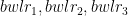
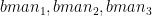
Assume there are 3 bowlers – and there are 3 batsmen –
I) LP Formulation for bowling order
Let the economy rate be the Economy Rate of the jth bowler to the ith batsman. Also if remaining overs for the bowlers are and the total number of overs left to be bowled are
Let the economy rate be the Economy Rate of the jth bowler to the ith batsman. Objective function : Minimize – i.e. Constraints Where is the number of overs remaining for the jth bowler against ‘k’ batsmen and if the total number of overs remaining to be bowled is N then or The overs that any bowler can bowl is
II) LP Formulation for batting lineup
Let the strike rate be the Strike Rate of the ith batsman to the jth bowler Objective function : Maximize – i.e. Constraints Where is the number of overs remaining for the jth bowler against ‘k’ batsmen and the total number of overs remaining to be bowled is N then or The overs that any bowler can bowl is
C) Optimized bowling lineup
a) IPL – Optimizing bowling line up
Note: For computing the Optimal bowling lineup, the total number of overs remaining and the number of overs for each bowler have to be entered.
b) PSL – Optimizing batting line up
d) Optimized batting lineup
a) Intl. T20 (men) India vs England
b) Carribean Premier League – Optimizing batting line up
This latest edition of GooglyPlusPlus2021 now includes detailed analysis of teams, batsmen and bowlers in power play, middle and death overs. The T20 format is based on 3 phases as each side faces 20 overs.
Power play: Overs: 0 – 6 – No more than 2 players can be outside the 30 yard circle
Middle overs: Overs: 7- 16 – During these overs the batting side tries to consolidate their innings
Death overs: Overs: 16 -20 – During these 5 overs the batting side tries to accelerate the scoring rate, while the bowling side will try to restrict the batsmen against going for big hits
This is shown below
This latest update of GooglyPlusPlus2021 includes the following functions
a) Match tab
teamRunsAcrossOvers
teamSRAcrossOvers
teamWicketsAcrossOvers
teamERAcrossOvers
matchWormWickets
b) Head-to-head tab
teamRunsAcrossOversOppnAllMatches
teamSRAcrossOversOppnAllMatches
teamWicketsAcrossOversOppnAllMatches
teamERAcrossOversOppnAllMatches
topRunsBatsmenAcrossOversOppnAllMatches
topSRBatsmenAcrossOversOppnAllMatches
topWicketsBowlersAcrossOversOppnAllMatches
topERBowlerAcrossOverOppnAllMatches
c) Overall performance tab
teamRunsAcrossOversAllOppnAllMatches
teamSRAcrossOversAllOppnAllMatches
teamWicketsAcrossOversAllOppnAllMatches
teamERAcrossOversAllOppnAllMatches
topRunsBatsmenAcrossOversAllOppnAllMatches
topSRBatsmenAcrossOversAllOppnAllMatches
topWicketsBowlersAcrossOversAllOppnAllMatches
topERBowlerAcrossOverAllOppnAllMatches
Hence a total of 8 + 8 + 5 = 21 functions have been added. These functions can be utilized across all the 9 T20 formats that are supported in GooglyPlusPlus2021 namely
You can clone/fork the code for the Shiny app from Github – gpp2021-9
Included below is a random selection of options from the 189 possibilities mentioned above. Feel free to try out for yourself
A) IPL – CSK vs KKR 2018-04-10
a) Team Runs in power play, middle and death overs
b) Team Strike rate in power play, middle and death overs
B) Intl. T20 (men) – India vs Afghanistan (2021-11-03)
a) Team wickets in power play, middle and death overs
b) Team Economy rate in power play, middle and death overs
C) Intl. T20 (women) Head-to-head : India vs Australia since 2018
a) Team Runs in all matches in power play, middle and death overs
D) PSL Head-to-head strike rate since 2019
a) Team vs team Strike rate : Karachi Kings vs Lahore Qalanders since 2019 in power play, middle and death overs
E) Team overall performance in all matches against all opposition
a) BBL : Brisbane Heats : Team Wickets between 2015 – 2018 in power play, middle and death overs
F) Top Runs and Strike rate Batsman of Mumbai Indians vs Royal Challengers Bangalore since 2018
a) Top runs scorers for Mumbai Indians (MI) in power play, middle and death overs
b) Top strike rate for RCB in power play, middle and death overs
F) Intl. T20 (women) India vs England since 2018
a) Top wicket takers for England in power play, middle and death overs since 2018
b) Top wicket takers for India in power play, middle and death overs since 2018
G) Intl. T20 (men) All time best batsmen and bowlers for India
a) Most runs in power play, middle and death overs
b) Highest strike rate in power play, middle and death overs
H) Match worm wicket chart
In addition to the usual Match worm chart, I have also added a Match Wicket worm chart in the latest version
Note: You can zoom to the area where you would like to focus more
The option of looking at the Match worm chart (without wickets) also exists.
Go ahead take GooglyPlusPlus2021 for a test drive and check out how your favourite players perform in power play, middle and death overs. Click GooglyPlusPlus2021
You can fork/download the app code from Github at gpp2021-9
This year 2021, we are witnessing a rare spectacle in the cricketing universe, where IPL playoffs are immediately followed by ICC World Cup T20. Cricket pundits have claimed such a phenomenon occurs once in 127 years! Jokes apart, the World cup T20 is underway and as usual GooglyPlusPlus is ready for the action.
GooglyPlusPlus will provide near-real time analytics, by automatically downloading the latest match data daily, processing and organising the match data into appropriate folders so that my R package yorkr can slice and dice the data to provide the pavilion-view analytics.
The charts capture all the breathless, heart-pounding, and nail-biting action in great details in the many tables and plots. Every table and chart tell a story. You just have to ‘read between the lines!’
GooglyPlusPlus2021 will update itself automatically every day, so the data will be current and you can analyse all matches upto the previous day, along with the historical performances of the teams. So make sure you check it everyday.
The are 5 tabs for each of the formats supported by GooglyPlusPlus2021 which now supports IPL, Intl. T20(men), Intl. T20(women), BBL, NTB, PSL, CPL, SSM, WBB. Besides, it also supports ODI (men) and ODI (women)
Each of the formats have 5 tabs – Batsman, Bowler, Match, Head-to-head and Overall Performace.
All T20 formats also include a ranking functionality for the batsmen and bowlers
You can now perform drill-down analytics for batsmen, bowlers, head-to-head and overall performance based on date-range selector functionality. The ranking tabs also include date range selector granular analysis. For more details see GooglyPlusPlus2021 enhanced with drill-down batsman, bowler analytics
This latest update of GooglyPlusPlus2021 includes new controls which allow for granular analysis of teams and matches. This version includes a new ‘Date Range’ widget which will allow you to choose a specific interval between which you would like to analyze data. The Date Range widget has been added to 2 tabs namely
a) Head-to-Head
b) Overall Performance
Important note:
This change is applicable to all T20 formats and ODI formats that GooglyPlusPlus2021 handles. This means you can do fine-grained analysis of the following formats
a. IPL b. Intl. T20 (men) c. Intl. T20 (women)
d. BBL e. NTB f. PSL
g. WBB h. CPL i. SSM
j. ODI (men) k. ODI (women)
Important note 1: Also note that all charts in GooglyPlusPlus2021 are interactive. You ca hover over the charts to get details of the data below. You can also selectively filter in bar charts using double-click and click. To know more about how to use GooglyPlusPlus2021 interactively, please see my post GooglyPlusPlus2021 is now fully interactive!!
You can clone/download the code for GooglyPlusPlus2021 from Github at GooglyPlusPlus2021


 be the Economy Rate of the jth bowler to the ith batsman. Also if remaining overs for the bowlers are


 is the number of overs remaining for the jth bowler against ‘k’ batsmen
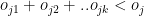
 or
or

 be the Strike Rate of the ith batsman to the jth bowler


