Rlanguage – Giga thoughts …

In this 4th post of my series on Deep Learning from first principles in Python, R and Octave – Part 4, I explore the details of creating a multi-class classifier using the Softmax activation unit in a neural network. The earlier posts in this series were

1. Deep Learning from first principles in Python, R and Octave – Part 1. In this post I implemented logistic regression as a simple Neural Network in vectorized Python, R and Octave
2. Deep Learning from first principles in Python, R and Octave – Part 2. This 2nd part implemented the most elementary neural network with 1 hidden layer and any number of activation units in the hidden layer with sigmoid activation at the output layer
3. Deep Learning from first principles in Python, R and Octave – Part 3. The 3rd implemented a multi-layer Deep Learning network with an arbitrary number if hidden layers and activation units per hidden layer. The output layer was for binary classification which was based on the sigmoid unit. This multi-layer deep network was implemented in vectorized Python, R and Octave.

Checkout my book ‘Deep Learning from first principles: Second Edition – In vectorized Python, R and Octave’. My book starts with the implementation of a simple 2-layer Neural Network and works its way to a generic L-Layer Deep Learning Network, with all the bells and whistles. The derivations have been discussed in detail. The code has been extensively commented and included in its entirety in the Appendix sections. My book is available on Amazon as paperback ($18.99) and in kindle version($9.99/Rs449).

This 4th part takes a swing at multi-class classification and uses the Softmax as the activation unit in the output layer. Inclusion of the Softmax activation unit in the activation layer requires us to compute the derivative of Softmax, or rather the “Jacobian” of the Softmax function, besides also computing the log loss for this Softmax activation during back propagation. Since the derivation of the Jacobian of a Softmax and the computation of the Cross Entropy/log loss is very involved, I have implemented a basic neural network with just 1 hidden layer with the Softmax activation at the output layer. I also perform multi-class classification based on the ‘spiral’ data set from CS231n Convolutional Neural Networks Stanford course, to test the performance and correctness of the implementations in Python, R and Octave. You can clone download the code for the Python, R and Octave implementations from Github at Deep Learning – Part 4

Note: A detailed discussion of the derivation below can also be seen in my video presentation Neural Networks 5

The Softmax function takes an N dimensional vector as input and generates a N dimensional vector as output.
The Softmax function is given by
$S_{j}= \frac{e_{j}}{\sum_{i}^{N}e_{k}}$
There is a probabilistic interpretation of the Softmax, since the sum of the Softmax values of a set of vectors will always add up to 1, given that each Softmax value is divided by the total of all values.

As mentioned earlier, the Softmax takes a vector input and returns a vector of outputs. For e.g. the Softmax of a vector a=[1, 3, 6] is another vector S=[0.0063,0.0471,0.9464]. Notice that vector output is proportional to the input vector. Also, taking the derivative of a vector by another vector, is known as the Jacobian. By the way, The Matrix Calculus You Need For Deep Learning by Terence Parr and Jeremy Howard, is very good paper that distills all the main mathematical concepts for Deep Learning in one place.

Let us take a simple 2 layered neural network with just 2 activation units in the hidden layer is shown below

$Z_{1}^{1} =W_{11}^{1}x_{1} + W_{21}^{1}x_{2} + b_{1}^{1}$
$Z_{2}^{1} =W_{12}^{1}x_{1} + W_{22}^{1}x_{2} + b_{2}^{1}$
and
$A_{1}^{1} = g'(Z_{1}^{1})$
$A_{2}^{1} = g'(Z_{2}^{1})$
where g'() is the activation unit in the hidden layer which can be a relu, sigmoid or a
tanh function

Note: The superscript denotes the layer. The above denotes the equation for layer 1
of the neural network. For layer 2 with the Softmax activation, the equations are
$Z_{1}^{2} =W_{11}^{2}x_{1} + W_{21}^{2}x_{2} + b_{1}^{2}$
$Z_{2}^{2} =W_{12}^{2}x_{1} + W_{22}^{2}x_{2} + b_{2}^{2}$
and
$A_{1}^{2} = S(Z_{1}^{2})$
$A_{2}^{2} = S(Z_{2}^{2})$
where S() is the Softmax activation function
$S=\begin{pmatrix} S(Z_{1}^{2})\\ S(Z_{2}^{2}) \end{pmatrix}$
$S=\begin{pmatrix} \frac{e^{Z1}}{e^{Z1}+e^{Z2}}\\ \frac{e^{Z2}}{e^{Z1}+e^{Z2}} \end{pmatrix}$

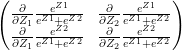
The Jacobian of the softmax ‘S’ is given by
$\begin{pmatrix} \frac {\partial S_{1}}{\partial Z_{1}} & \frac {\partial S_{1}}{\partial Z_{2}}\\ \frac {\partial S_{2}}{\partial Z_{1}} & \frac {\partial S_{2}}{\partial Z_{2}} \end{pmatrix}$
$\begin{pmatrix} \frac{\partial}{\partial Z_{1}} \frac {e^{Z1}}{e^{Z1}+ e^{Z2}} & \frac{\partial}{\partial Z_{2}} \frac {e^{Z1}}{e^{Z1}+ e^{Z2}}\\ \frac{\partial}{\partial Z_{1}} \frac {e^{Z2}}{e^{Z1}+ e^{Z2}} & \frac{\partial}{\partial Z_{2}} \frac {e^{Z2}}{e^{Z1}+ e^{Z2}} \end{pmatrix}$ – (A)

Now the ‘division-rule’ of derivatives is as follows. If u and v are functions of x, then
$\frac{d}{dx} \frac {u}{v} =\frac {vdu -udv}{v^{2}}$
Using this to compute each element of the above Jacobian matrix, we see that
when i=j we have
$\frac {\partial}{\partial Z1}\frac{e^{Z1}}{e^{Z1}+e^{Z2}} = \frac {\sum e^{Z1} - e^{Z1^{2}}}{\sum ^{2}}$
and when $i \neq j$
$\frac {\partial}{\partial Z1}\frac{e^{Z2}}{e^{Z1}+e^{Z2}} = \frac {0 - e^{z1}e^{Z2}}{\sum ^{2}}$
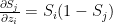
This is of the general form
$\frac {\partial S_{j}}{\partial z_{i}} = S_{i}( 1-S_{j})$ when i=j
and
$\frac {\partial S_{j}}{\partial z_{i}} = -S_{i}S_{j}$ when $i \neq j$
Note: Since the Softmax essentially gives the probability the following
notation is also used
$\frac {\partial p_{j}}{\partial z_{i}} = p_{i}( 1-p_{j})$ when i=j
and
$\frac {\partial p_{j}}{\partial z_{i}} = -p_{i}p_{j} when i \neq j$
If you throw the “Kronecker delta” into the equation, then the above equations can be expressed even more concisely as
$\frac {\partial p_{j}}{\partial z_{i}} = p_{i} (\delta_{ij} - p_{j})$
where $\delta_{ij} = 1$ when i=j and 0 when $i \neq j$

This reduces the Jacobian of the simple 2 output softmax vectors equation (A) as
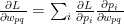
$\begin{pmatrix} p_{1}(1-p_{1}) & -p_{1}p_{2} \\ -p_{2}p_{1} & p_{2}(1-p_{2}) \end{pmatrix}$
The loss of Softmax is given by
$L = -\sum y_{i} log(p_{i})$
For the 2 valued Softmax output this is
$\frac {dL}{dp1} = -\frac {y_{1}}{p_{1}}$
$\frac {dL}{dp2} = -\frac {y_{2}}{p_{2}}$
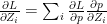
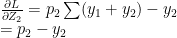
Using the chain rule we can write
$\frac {\partial L}{\partial w_{pq}} = \sum _{i}\frac {\partial L}{\partial p_{i}} \frac {\partial p_{i}}{\partial w_{pq}}$ (1)
and
$\frac {\partial p_{i}}{\partial w_{pq}} = \sum _{k}\frac {\partial p_{i}}{\partial z_{k}} \frac {\partial z_{k}}{\partial w_{pq}}$ (2)
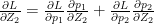
In expanded form this is
$\frac {\partial L}{\partial w_{pq}} = \sum _{i}\frac {\partial L}{\partial p_{i}} \sum _{k}\frac {\partial p_{i}}{\partial z_{k}} \frac {\partial z_{k}}{\partial w_{pq}}$
Also
$\frac {\partial L}{\partial Z_{i}} =\sum _{i} \frac {\partial L}{\partial p} \frac {\partial p}{\partial Z_{i}}$
Therefore
$\frac {\partial L}{\partial Z_{1}} =\frac {\partial L}{\partial p_{1}} \frac {\partial p_{1}}{\partial Z_{1}} +\frac {\partial L}{\partial p_{2}} \frac {\partial p_{2}}{\partial Z_{1}}$
$\frac {\partial L}{\partial z_{1}}=-\frac {y1}{p1} p1(1-p1) - \frac {y2}{p2}*(-p_{2}p_{1})$
Since
$\frac {\partial p_{j}}{\partial z_{i}} = p_{i}( 1-p_{j})$ when i=j
and
$\frac {\partial p_{j}}{\partial z_{i}} = -p_{i}p_{j}$ when $i \neq j$
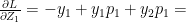
which simplifies to
$\frac {\partial L}{\partial Z_{1}} = -y_{1} + y_{1}p_{1} + y_{2}p_{1} =$
$p_{1}\sum (y_{1} + y_2) - y_{1}$
$\frac {\partial L}{\partial Z_{1}}= p_{1} - y_{1}$
Since
$\sum_{i} y_{i} =1$
Similarly
$\frac {\partial L}{\partial Z_{2}} =\frac {\partial L}{\partial p_{1}} \frac {\partial p_{1}}{\partial Z_{2}} +\frac {\partial L}{\partial p_{2}} \frac {\partial p_{2}}{\partial Z_{2}}$
$\frac {\partial L}{\partial z_{2}}=-\frac {y1}{p1}*(p_{1}p_{2}) - \frac {y2}{p2}*p_{2}(1-p_{2})$
$y_{1}p_{2} + y_{2}p_{2} - y_{2}$
$\frac {\partial L}{\partial Z_{2}} =p_{2}\sum (y_{1} + y_2) - y_{2}\\ = p_{2} - y_{2}$
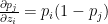
In general this is of the form
$\frac {\partial L}{\partial z_{i}} = p_{i} -y_{i}$
For e.g if the probabilities computed were p=[0.1, 0.7, 0.2] then this implies that the class with probability 0.7 is the likely class. This would imply that the ‘One hot encoding’ for yi would be yi=[0,1,0] therefore the gradient pi-yi = [0.1,-0.3,0.2]

<strong>Note: Further, we could extend this derivation for a Softmax activation output that outputs 3 classes
$S=\begin{pmatrix} \frac{e^{z1}}{e^{z1}+e^{z2}+e^{z3}}\\ \frac{e^{z2}}{e^{z1}+e^{z2}+e^{z3}} \\ \frac{e^{z3}}{e^{z1}+e^{z2}+e^{z3}} \end{pmatrix}$

We could derive
$\frac {\partial L}{\partial z1}= \frac {\partial L}{\partial p_{1}} \frac {\partial p_{1}}{\partial z_{1}} +\frac {\partial L}{\partial p_{2}} \frac {\partial p_{2}}{\partial z_{1}} +\frac {\partial L}{\partial p_{3}} \frac {\partial p_{3}}{\partial z_{1}}$ which similarly reduces to
$\frac {\partial L}{\partial z_{1}}=-\frac {y1}{p1} p1(1-p1) - \frac {y2}{p2}*(-p_{2}p_{1}) - \frac {y3}{p3}*(-p_{3}p_{1})$
$-y_{1}+ y_{1}p_{1} + y_{2}p_{1} + y_{3}p1 = p_{1}\sum (y_{1} + y_2 + y_3) - y_{1} = p_{1} - y_{1}$
Interestingly, despite the lengthy derivations the final result is simple and intuitive!

As seen in my post ‘Deep Learning from first principles with Python, R and Octave – Part 3 the key equations for forward and backward propagation are

Forward propagation equations layer 1
$Z_{1} = W_{1}X +b_{1}$ and $A_{1} = g(Z_{1})$
Forward propagation equations layer 1
$Z_{2} = W_{2}A_{1} +b_{2}$ and $A_{2} = S(Z_{2})$

Using the result (A) in the back propagation equations below we have
Backward propagation equations layer 2
$\partial L/\partial W_{2} =\partial L/\partial Z_{2}*A_{1}=(p_{2}-y_{2})*A_{1}$
$\partial L/\partial b_{2} =\partial L/\partial Z_{2}=p_{2}-y_{2}$
$\partial L/\partial A_{1} = \partial L/\partial Z_{2} * W_{2}=(p_{2}-y_{2})*W_{2}$
Backward propagation equations layer 1
$\partial L/\partial W_{1} =\partial L/\partial Z_{1} *A_{0}=(p_{1}-y_{1})*A_{0}$
$\partial L/\partial b_{1} =\partial L/\partial Z_{1}=(p_{1}-y_{1})$

2.0 Spiral data set

As I mentioned earlier, I will be using the ‘spiral’ data from CS231n Convolutional Neural Networks to ensure that my vectorized implementations in Python, R and Octave are correct. Here is the ‘spiral’ data set.

import numpy as np
import matplotlib.pyplot as plt
import os
os.chdir("C:/junk/dl-4/dl-4")
exec(open("././DLfunctions41.py").read())

# Create an input data set - Taken from CS231n Convolutional Neural networks
# http://cs231n.github.io/neural-networks-case-study/
N = 100 # number of points per class
D = 2 # dimensionality
K = 3 # number of classes
X = np.zeros((N*K,D)) # data matrix (each row = single example)
y = np.zeros(N*K, dtype='uint8') # class labels
for j in range(K):
  ix = range(N*j,N*(j+1))
  r = np.linspace(0.0,1,N) # radius
  t = np.linspace(j*4,(j+1)*4,N) + np.random.randn(N)*0.2 # theta
  X[ix] = np.c_[r*np.sin(t), r*np.cos(t)]
  y[ix] = j
# Plot the data
plt.scatter(X[:, 0], X[:, 1], c=y, s=40, cmap=plt.cm.Spectral)
plt.savefig("fig1.png", bbox_inches='tight')

The implementations of the vectorized Python, R and Octave code are shown diagrammatically below

2.1 Multi-class classification with Softmax – Python code

A simple 2 layer Neural network with a single hidden layer , with 100 Relu activation units in the hidden layer and the Softmax activation unit in the output layer is used for multi-class classification. This Deep Learning Network, plots the non-linear boundary of the 3 classes as shown below

import numpy as np
import matplotlib.pyplot as plt
import os
os.chdir("C:/junk/dl-4/dl-4")
exec(open("././DLfunctions41.py").read())

# Read the input data
N = 100 # number of points per class
D = 2 # dimensionality
K = 3 # number of classes
X = np.zeros((N*K,D)) # data matrix (each row = single example)
y = np.zeros(N*K, dtype='uint8') # class labels
for j in range(K):
  ix = range(N*j,N*(j+1))
  r = np.linspace(0.0,1,N) # radius
  t = np.linspace(j*4,(j+1)*4,N) + np.random.randn(N)*0.2 # theta
  X[ix] = np.c_[r*np.sin(t), r*np.cos(t)]
  y[ix] = j
  
# Set the number of features, hidden units in hidden layer and number of classess
numHidden=100 # No of hidden units in hidden layer
numFeats= 2 # dimensionality
numOutput = 3 # number of classes

# Initialize the model
parameters=initializeModel(numFeats,numHidden,numOutput)
W1= parameters['W1']
b1= parameters['b1']
W2= parameters['W2']
b2= parameters['b2']

# Set the learning rate
learningRate=0.6 

# Initialize losses
losses=[]
# Perform Gradient descent
for i in range(10000):
    # Forward propagation through hidden layer with Relu units
    A1,cache1= layerActivationForward(X.T,W1,b1,'relu')
    
    # Forward propagation through output layer with Softmax
    A2,cache2 = layerActivationForward(A1,W2,b2,'softmax')
    
    # No of training examples
    numTraining = X.shape[0]
    # Compute log probs. Take the log prob of correct class based on output y
    correct_logprobs = -np.log(A2[range(numTraining),y])
    # Conpute loss
    loss = np.sum(correct_logprobs)/numTraining
    
    # Print the loss
    if i % 1000 == 0:
        print("iteration %d: loss %f" % (i, loss))
        losses.append(loss)

    dA=0

    # Backward  propagation through output layer with Softmax
    dA1,dW2,db2 = layerActivationBackward(dA, cache2, y, activationFunc='softmax')
    # Backward  propagation through hidden layer with Relu unit
    dA0,dW1,db1 = layerActivationBackward(dA1.T, cache1, y, activationFunc='relu')
    
    #Update paramaters with the learning rate
    W1 += -learningRate * dW1
    b1 += -learningRate * db1
    W2 += -learningRate * dW2.T
    b2 += -learningRate * db2.T

#Plot losses vs iterations  
i=np.arange(0,10000,1000)
plt.plot(i,losses)

plt.xlabel('Iterations')
plt.ylabel('Loss')
plt.title('Losses vs Iterations')
plt.savefig("fig2.png", bbox="tight")

#Compute the multi-class Confusion Matrix
from sklearn.metrics import confusion_matrix
from sklearn.metrics import accuracy_score, precision_score, recall_score, f1_score

# We need to determine the predicted values from the learnt data
# Forward propagation through hidden layer with Relu units
A1,cache1= layerActivationForward(X.T,W1,b1,'relu')
    
# Forward propagation through output layer with Softmax
A2,cache2 = layerActivationForward(A1,W2,b2,'softmax')
#Compute predicted values from weights and biases
yhat=np.argmax(A2, axis=1)

a=confusion_matrix(y.T,yhat.T)
print("Multi-class Confusion Matrix")
print(a)

## iteration 0: loss 1.098507
## iteration 1000: loss 0.214611
## iteration 2000: loss 0.043622
## iteration 3000: loss 0.032525
## iteration 4000: loss 0.025108
## iteration 5000: loss 0.021365
## iteration 6000: loss 0.019046
## iteration 7000: loss 0.017475
## iteration 8000: loss 0.016359
## iteration 9000: loss 0.015703
## Multi-class Confusion Matrix
## [[ 99   1   0]
##  [  0 100   0]
##  [  0   1  99]]

Check out my compact and minimal book “Practical Machine Learning with R and Python:Second edition- Machine Learning in stereo” available in Amazon in paperback($10.99) and kindle($7.99) versions. My book includes implementations of key ML algorithms and associated measures and metrics. The book is ideal for anybody who is familiar with the concepts and would like a quick reference to the different ML algorithms that can be applied to problems and how to select the best model. Pick your copy today!!

2.2 Multi-class classification with Softmax – R code

The spiral data set created with Python was saved, and is used as the input with R code. The R Neural Network seems to perform much,much slower than both Python and Octave. Not sure why! Incidentally the computation of loss and the softmax derivative are identical for both R and Octave. yet R is much slower. To compute the softmax derivative I create matrices for the One Hot Encoded yi and then stack them before subtracting pi-yi. I am sure there is a more elegant and more efficient way to do this, much like Python. Any suggestions?

library(ggplot2)
library(dplyr)
library(RColorBrewer)

source("DLfunctions41.R")
# Read the spiral dataset
Z <- as.matrix(read.csv("spiral.csv",header=FALSE)) 
Z1=data.frame(Z)
#Plot the dataset
ggplot(Z1,aes(x=V1,y=V2,col=V3)) +geom_point() + 
  scale_colour_gradientn(colours = brewer.pal(10, "Spectral"))

# Setup the data
X <- Z[,1:2]
y <- Z[,3]
X1 <- t(X)
Y1 <- t(y)

# Initialize number of features, number of hidden units in hidden layer and
# number of classes
numFeats<-2 # No features
numHidden<-100 # No of hidden units
numOutput<-3 # No of classes

# Initialize model
parameters <-initializeModel(numFeats, numHidden,numOutput)

W1 <-parameters[['W1']]
b1 <-parameters[['b1']]
W2 <-parameters[['W2']]
b2 <-parameters[['b2']]

# Set the learning rate
learningRate <- 0.5
# Initialize losses
losses <- NULL
# Perform gradient descent
for(i in 0:9000){

# Forward propagation through hidden layer with Relu units
retvals <- layerActivationForward(X1,W1,b1,'relu')
A1 <- retvals[['A']]
cache1 <- retvals[['cache']]
forward_cache1 <- cache1[['forward_cache1']]
activation_cache <- cache1[['activation_cache']]

# Forward propagation through output layer with Softmax units
retvals = layerActivationForward(A1,W2,b2,'softmax')
A2 <- retvals[['A']]
cache2 <- retvals[['cache']]
forward_cache2 <- cache2[['forward_cache1']]
activation_cache2 <- cache2[['activation_cache']]

# No oftraining examples
numTraining <- dim(X)[1]
dA <-0

# Select the elements where the y values are 0, 1 or 2 and make a vector
a=c(A2[y==0,1],A2[y==1,2],A2[y==2,3])
# Take log
correct_probs = -log(a)
# Compute loss
loss= sum(correct_probs)/numTraining

if(i %% 1000 == 0){
sprintf("iteration %d: loss %f",i, loss)
print(loss)
}
# Backward propagation through output layer with Softmax units
retvals = layerActivationBackward(dA, cache2, y, activationFunc='softmax')
dA1 = retvals[['dA_prev']]
dW2= retvals[['dW']]
db2= retvals[['db']]
# Backward propagation through hidden layer with Relu units
retvals = layerActivationBackward(t(dA1), cache1, y, activationFunc='relu')
dA0 = retvals[['dA_prev']]
dW1= retvals[['dW']]
db1= retvals[['db']]

# Update parameters
W1 <- W1 - learningRate * dW1
b1 <- b1 - learningRate * db1
W2 <- W2 - learningRate * t(dW2)
b2 <- b2 - learningRate * t(db2)
}

## [1] 1.212487
## [1] 0.5740867
## [1] 0.4048824
## [1] 0.3561941
## [1] 0.2509576
## [1] 0.7351063
## [1] 0.2066114
## [1] 0.2065875
## [1] 0.2151943
## [1] 0.1318807

#Create iterations
iterations <- seq(0,10)
#df=data.frame(iterations,losses)
ggplot(df,aes(x=iterations,y=losses)) + geom_point() + geom_line(color="blue") +
    ggtitle("Losses vs iterations") + xlab("Iterations") + ylab("Loss")

plotDecisionBoundary(Z,W1,b1,W2,b2)

Multi-class Confusion Matrix

library(caret)
library(e1071)

# Forward propagation through hidden layer with Relu units
retvals <- layerActivationForward(X1,W1,b1,'relu')
A1 <- retvals[['A']]

# Forward propagation through output layer with Softmax units
retvals = layerActivationForward(A1,W2,b2,'softmax')
A2 <- retvals[['A']]
yhat <- apply(A2, 1,which.max) -1
Confusion Matrix and Statistics
          Reference
Prediction  0  1  2
         0 97  0  1
         1  2 96  4
         2  1  4 95

Overall Statistics                                        
               Accuracy : 0.96            
                 95% CI : (0.9312, 0.9792)
    No Information Rate : 0.3333          
    P-Value [Acc > NIR] : <2e-16          
                                          
                  Kappa : 0.94            
 Mcnemar's Test P-Value : 0.5724          
Statistics by Class:

                     Class: 0 Class: 1 Class: 2
Sensitivity            0.9700   0.9600   0.9500
Specificity            0.9950   0.9700   0.9750
Pos Pred Value         0.9898   0.9412   0.9500
Neg Pred Value         0.9851   0.9798   0.9750
Prevalence             0.3333   0.3333   0.3333
Detection Rate         0.3233   0.3200   0.3167
Detection Prevalence   0.3267   0.3400   0.3333
Balanced Accuracy      0.9825   0.9650   0.9625

My book “Practical Machine Learning with R and Python” includes the implementation for many Machine Learning algorithms and associated metrics. Pick up your copy today!

2.3 Multi-class classification with Softmax – Octave code

A 2 layer Neural network with the Softmax activation unit in the output layer is constructed in Octave. The same spiral data set is used for Octave also
source("DL41functions.m") # Read the spiral data data=csvread("spiral.csv"); # Setup the data X=data(:,1:2); Y=data(:,3); # Set the number of features, number of hidden units in hidden layer and number of classes numFeats=2; #No features numHidden=100; # No of hidden units numOutput=3; # No of classes # Initialize model [W1 b1 W2 b2] = initializeModel(numFeats,numHidden,numOutput); # Initialize losses losses=[] #Initialize learningRate learningRate=0.5; for k =1:10000 # Forward propagation through hidden layer with Relu units [A1,cache1 activation_cache1]= layerActivationForward(X',W1,b1,activationFunc ='relu'); # Forward propagation through output layer with Softmax units [A2,cache2 activation_cache2] = layerActivationForward(A1,W2,b2,activationFunc='softmax'); # No of training examples numTraining = size(X)(1); # Select rows where Y=0,1,and 2 and concatenate to a long vector a=[A2(Y==0,1) ;A2(Y==1,2) ;A2(Y==2,3)]; #Select the correct column for log prob correct_probs = -log(a); #Compute log loss loss= sum(correct_probs)/numTraining; if(mod(k,1000) == 0) disp(loss); losses=[losses loss]; endif dA=0; # Backward propagation through output layer with Softmax units [dA1 dW2 db2] = layerActivationBackward(dA, cache2, activation_cache2,Y,activationFunc='softmax'); # Backward propagation through hidden layer with Relu units [dA0,dW1,db1] = layerActivationBackward(dA1', cache1, activation_cache1, Y, activationFunc='relu'); #Update parameters W1 += -learningRate * dW1; b1 += -learningRate * db1; W2 += -learningRate * dW2'; b2 += -learningRate * db2'; endfor # Plot Losses vs Iterations iterations=0:1000:9000 plotCostVsIterations(iterations,losses) # Plot the decision boundary plotDecisionBoundary( X,Y,W1,b1,W2,b2)

The code for the Python, R and Octave implementations can be downloaded from Github at Deep Learning – Part 4

Conclusion

In this post I have implemented a 2 layer Neural Network with the Softmax classifier. In Part 3, I implemented a multi-layer Deep Learning Network. I intend to include the Softmax activation unit into the generalized multi-layer Deep Network along with the other activation units of sigmoid,tanh and relu.

Stick around, I’ll be back!!
Watch this space!

References
1. Deep Learning Specialization
2. Neural Networks for Machine Learning
3. CS231 Convolutional Neural Networks for Visual Recognition
4. Eli Bendersky’s Website – The Softmax function and its derivative
5. Cross Validated – Backpropagation with Softmax / Cross Entropy
6. Stackoverflow – CS231n: How to calculate gradient for Softmax loss function?
7. Math Stack Exchange – Derivative of Softmax
8. The Matrix Calculus for Deep Learning