Here is the 1st part of my video presentation on “Machine Learning, Data Science, NLP and Big Data – Part 2”
Category: linear regression

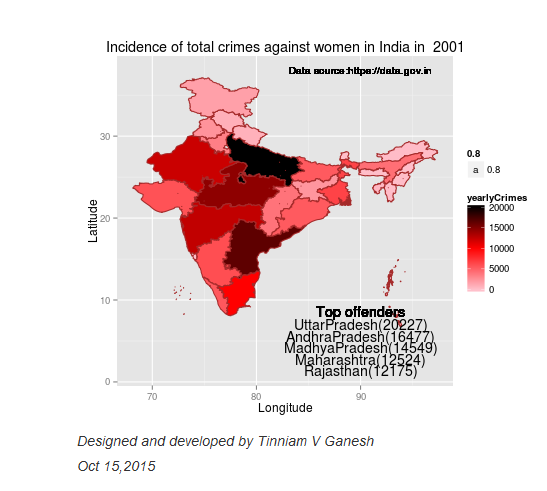
Revisiting crimes against women in India
Here I go again, raking the muck about crimes against women in India. My earlier post “A crime map of India in R: Crimes against women in India” garnered a lot of responses from readers. In fact one of the readers even volunteered to create the only choropleth map in that post. The data for this post is taken from http://data.gov.in. You can download the data from the link “Crimes against women in India”
I was so impressed by the choropleth map that I decided to do that for all crimes against women.(Wikipedia definition: A choropleth map is a thematic map in which areas are shaded or patterned in proportion to the measurement of the statistical variable being displayed on the map). Personally, I think pictures tell the story better. I am sure you will agree!
So here, I have it a Shiny app which will plot choropleth maps for a chosen crime in a given year.
You can try out my interactive Shiny app at Crimes against women in India
Checkout out my book on Amazon available in both Paperback ($9.99) and a Kindle version($6.99/Rs449/). (see ‘Practical Machine Learning with R and Python – Machine Learning in stereo‘)

The following technique can be used to determine the ‘goodness’ of a hypothesis or how well the hypothesis can fit the data and can also generalize to new examples not in the training set.
In the picture below are the details of ‘Rape” in the year 2015.

Interestingly the ‘Total Crime against women’ in 2001 shows the Top 5 as
1) Uttar Pradresh 2) Andhra Pradesh 3) Madhya Pradesh 4) Maharashtra 5) Rajasthan
But in 2015 West Bengal tops the list, as the real heavy weight in crimes against women. The new pecking order in 2015 for ‘Total Crimes against Women’ is
1) West Bengal 2) Andhra Pradesh 3) Uttar Pradesh 4) Rajasthan 5) Maharashtra

Similarly for rapes, West Bengal is nowhere in the top 5 list in 2001. In 2015, it is in second only to the national rape leader Madhya Pradesh. Also in 2001 West Bengal is not in the top 5 for any of 6 crime heads. But in 2015, West Bengal is in the top 5 of 6 crime heads. The emergence of West Bengal as the leader in Crimes against Women is due to the steep increase in crime rate over the years.Clearly the law and order situation in West Bengal is heading south.
In Dowry Deaths, UP, Bihar, MP, West Bengal lead the pack, and in that order in 2015.
The usual suspects for most crime categories are West Bengal, UP, MP, AP & Maharashtra.
The state-wise crime charts plot the incidence of the crime (rape, dowry death, assault on women etc) over the years. Data for each state and for each crime was available from 2001-2013. The data for period 2014-2018 are projected using linear regression. The shaded portion in the plots indicate the 95% confidence level in the prediction (i.e in other words we can be 95% certain that the true mean of the crime rate in the projected years will lie within the shaded region)

Several interesting requests came from readers to my earlier post. Some of them were to to plot the crimes as function of population and per capita income of the State/Union Territory to see if the plots throw up new crime leaders. I have not got the relevant state-wise population distribution data yet. I intend to update this when I get my hands on this data.
I have included the crimes.csv which has been used to generate the visualization. However for the Shiny app I save this as .RData for better performance of the app.
You can clone/download the code for the Shiny app from GitHub at crimesAgainWomenIndia
Please checkout my Shiny app : Crimes against women
I also intend to add further interactivity to my visualizations in a future version. Watch this space. I’ll be back!
You may like
1. My book ‘Practical Machine Learning with R and Python’ on Amazon
2. Natural Language Processing: What would Shakespeare say?
3. Introducing cricketr! : An R package to analyze performances of cricketers
4. A peek into literacy in India: Statistical Learning with R
5. Informed choices through Machine Learning : Analyzing Kohli, Tendulkar and Dravid
6. Re-working the Lucy-Richardson Algorithm in OpenCV
7. What’s up Watson? Using IBM Watson’s QAAPI with Bluemix, NodeExpress – Part 1
8. Bend it like Bluemix, MongoDB with autoscaling – Part 2
9. TWS-4: Gossip protocol: Epidemics and rumors to the rescue
10. Thinking Web Scale (TWS-3): Map-Reduce – Bring compute to data
11. Simulating an Edge Shape in Android
Share:

cricketr plays the ODIs!
Published in R bloggers: cricketr plays the ODIs
Introduction
In this post my package ‘cricketr’ takes a swing at One Day Internationals(ODIs). Like test batsman who adapt to ODIs with some innovative strokes, the cricketr package has some additional functions and some modified functions to handle the high strike and economy rates in ODIs. As before I have chosen my top 4 ODI batsmen and top 4 ODI bowlers.

If you are passionate about cricket, and love analyzing cricket performances, then check out my racy book on cricket ‘Cricket analytics with cricketr and cricpy – Analytics harmony with R & Python’! This book discusses and shows how to use my R package ‘cricketr’ and my Python package ‘cricpy’ to analyze batsmen and bowlers in all formats of the game (Test, ODI and T20). The paperback is available on Amazon at $21.99 and the kindle version at $9.99/Rs 449/-. A must read for any cricket lover! Check it out!!
You can download the latest PDF version of the book at ‘Cricket analytics with cricketr and cricpy: Analytics harmony with R and Python-6th edition‘

Important note 1: The latest release of ‘cricketr’ now includes the ability to analyze performances of teams now!! See Cricketr adds team analytics to its repertoire!!!
Important note 2 : Cricketr can now do a more fine-grained analysis of players, see Cricketr learns new tricks : Performs fine-grained analysis of players
Important note 3: Do check out the python avatar of cricketr, ‘cricpy’ in my post ‘Introducing cricpy:A python package to analyze performances of cricketers”
Do check out my interactive Shiny app implementation using the cricketr package – Sixer – R package cricketr’s new Shiny avatar
You can also read this post at Rpubs as odi-cricketr. Dowload this report as a PDF file from odi-cricketr.pdf
Important note: Do check out my other posts using cricketr at cricketr-posts
Note: If you would like to do a similar analysis for a different set of batsman and bowlers, you can clone/download my skeleton cricketr template from Github (which is the R Markdown file I have used for the analysis below). You will only need to make appropriate changes for the players you are interested in. Just a familiarity with R and R Markdown only is needed.
Batsmen
- Virendar Sehwag (Ind)
- AB Devilliers (SA)
- Chris Gayle (WI)
- Glenn Maxwell (Aus)
Bowlers
- Mitchell Johnson (Aus)
- Lasith Malinga (SL)
- Dale Steyn (SA)
- Tim Southee (NZ)
I have sprinkled the plots with a few of my comments. Feel free to draw your conclusions! The analysis is included below
The profile for Virender Sehwag is 35263. This can be used to get the ODI data for Sehwag. For a batsman the type should be “batting” and for a bowler the type should be “bowling” and the function is getPlayerDataOD()
The package can be installed directly from CRAN
if (!require("cricketr")){
    install.packages("cricketr",lib = "c:/test")
}
library(cricketr)
or from Github
library(devtools)
install_github("tvganesh/cricketr")
library(cricketr)
The One day data for a particular player can be obtained with the getPlayerDataOD() function. To do you will need to go to ESPN CricInfo Player and type in the name of the player for e.g Virendar Sehwag, etc. This will bring up a page which have the profile number for the player e.g. for Virendar Sehwag this would be http://www.espncricinfo.com/india/content/player/35263.html. Hence, Sehwag’s profile is 35263. This can be used to get the data for Virat Sehwag as shown below
sehwag <- getPlayerDataOD(35263,dir="..",file="sehwag.csv",type="batting")Analyses of Batsmen
The following plots gives the analysis of the 4 ODI batsmen
- Virendar Sehwag (Ind) – Innings – 245, Runs = 8586, Average=35.05, Strike Rate= 104.33
- AB Devilliers (SA) – Innings – 179, Runs= 7941, Average=53.65, Strike Rate= 99.12
- Chris Gayle (WI) – Innings – 264, Runs= 9221, Average=37.65, Strike Rate= 85.11
- Glenn Maxwell (Aus) – Innings – 45, Runs= 1367, Average=35.02, Strike Rate= 126.69
Plot of 4s, 6s and the scoring rate in ODIs
The 3 charts below give the number of
- 4s vs Runs scored
- 6s vs Runs scored
- Balls faced vs Runs scored
A regression line is fitted in each of these plots for each of the ODI batsmen A. Virender Sehwag
par(mfrow=c(1,3))
par(mar=c(4,4,2,2))
batsman4s("./sehwag.csv","Sehwag")
batsman6s("./sehwag.csv","Sehwag")
batsmanScoringRateODTT("./sehwag.csv","Sehwag")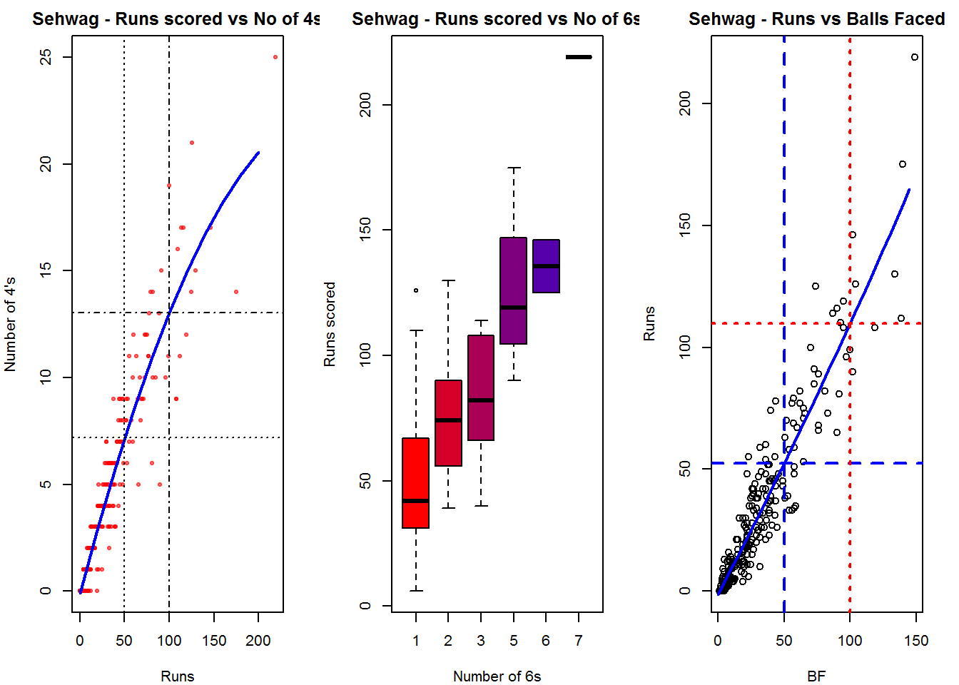
dev.off()## null device
## 1B. AB Devilliers
par(mfrow=c(1,3))
par(mar=c(4,4,2,2))
batsman4s("./devilliers.csv","Devillier")
batsman6s("./devilliers.csv","Devillier")
batsmanScoringRateODTT("./devilliers.csv","Devillier")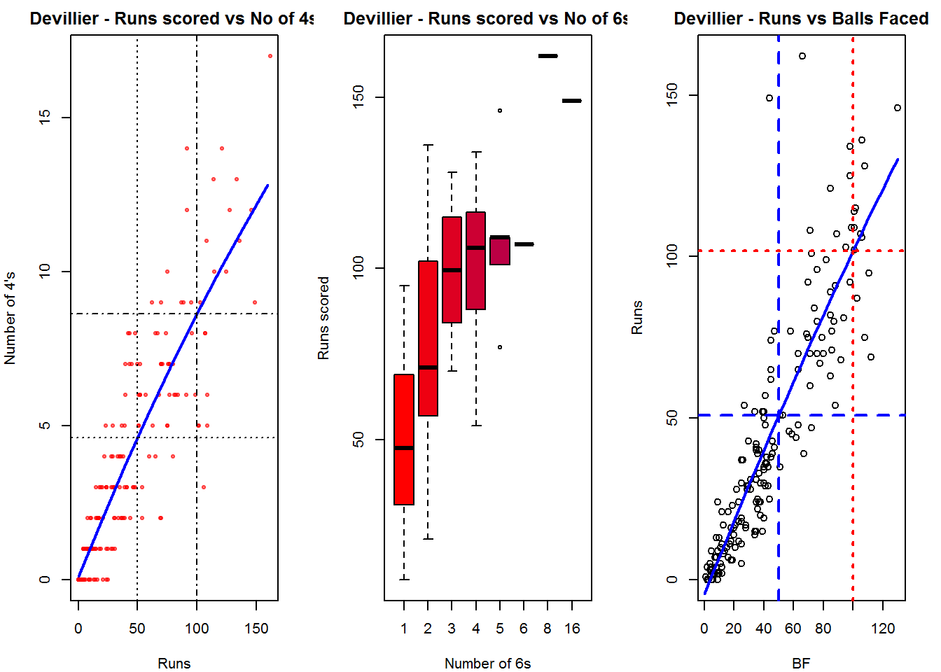
dev.off()## null device
## 1C. Chris Gayle
par(mfrow=c(1,3))
par(mar=c(4,4,2,2))
batsman4s("./gayle.csv","Gayle")
batsman6s("./gayle.csv","Gayle")
batsmanScoringRateODTT("./gayle.csv","Gayle")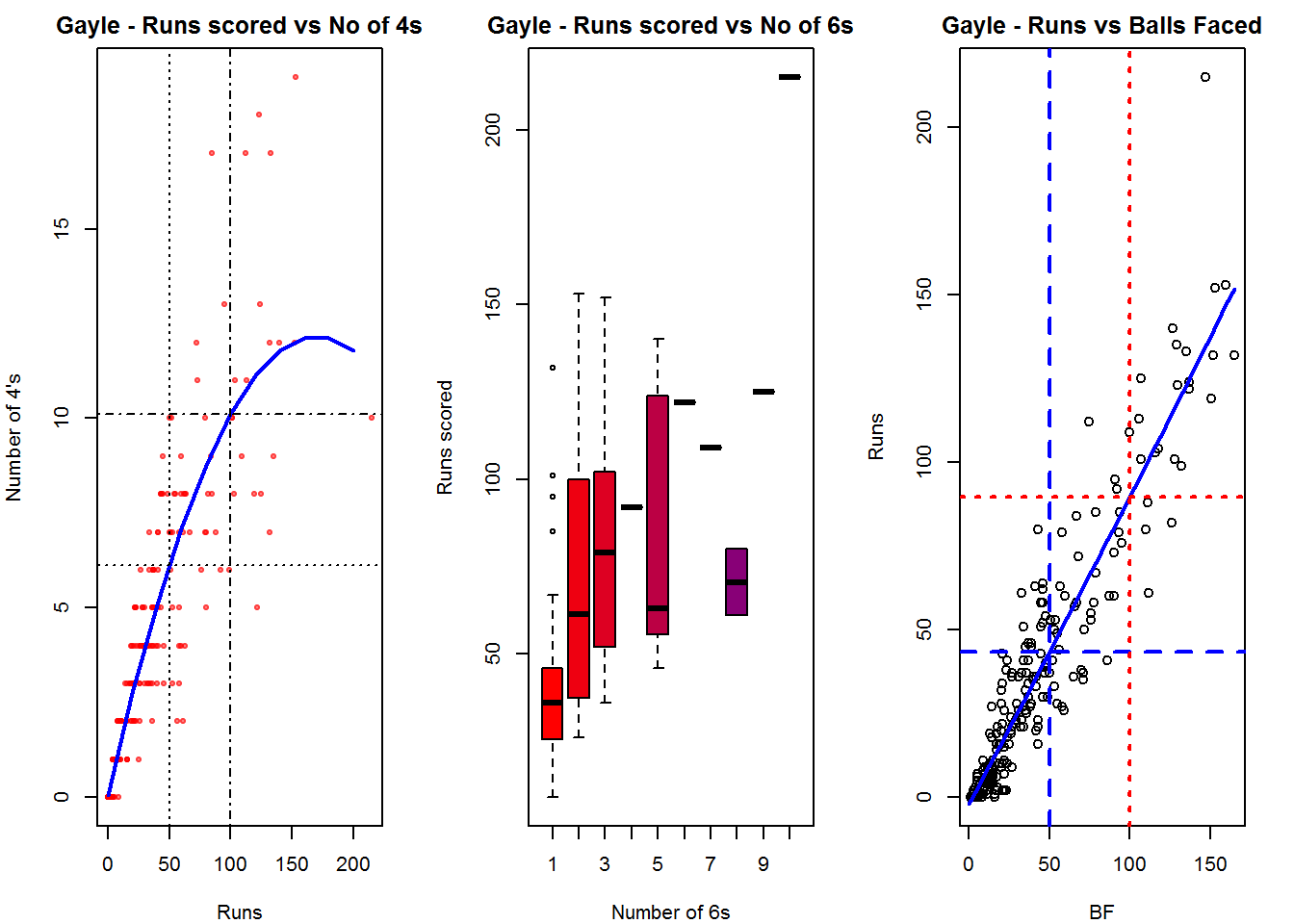
dev.off()## null device
## 1D. Glenn Maxwell
par(mfrow=c(1,3))
par(mar=c(4,4,2,2))
batsman4s("./maxwell.csv","Maxwell")
batsman6s("./maxwell.csv","Maxwell")
batsmanScoringRateODTT("./maxwell.csv","Maxwell")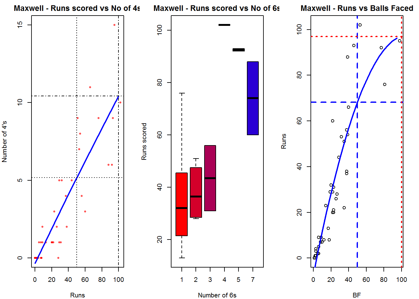
dev.off()## null device
## 1Relative Mean Strike Rate
In this first plot I plot the Mean Strike Rate of the batsmen. It can be seen that Maxwell has a awesome strike rate in ODIs. However we need to keep in mind that Maxwell has relatively much fewer (only 45 innings) innings. He is followed by Sehwag who(most innings- 245) also has an excellent strike rate till 100 runs and then we have Devilliers who roars ahead. This is also seen in the overall strike rate in above
par(mar=c(4,4,2,2))
frames <- list("./sehwag.csv","./devilliers.csv","gayle.csv","maxwell.csv")
names <- list("Sehwag","Devilliers","Gayle","Maxwell")
relativeBatsmanSRODTT(frames,names)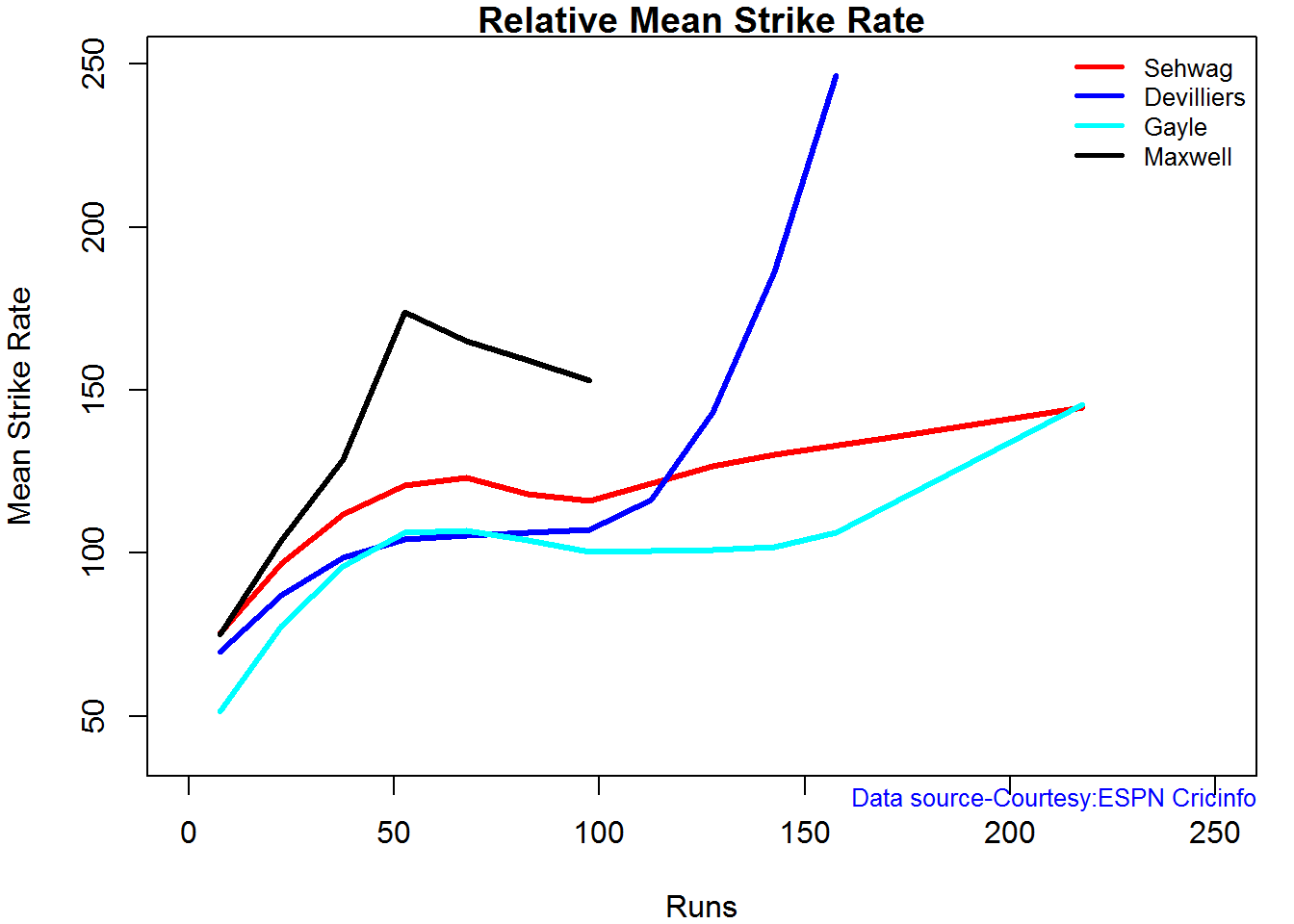
Relative Runs Frequency Percentage
Sehwag leads in the percentage of runs in 10 run ranges upto 50 runs. Maxwell and Devilliers lead in 55-66 & 66-85 respectively.
frames <- list("./sehwag.csv","./devilliers.csv","gayle.csv","maxwell.csv")
names <- list("Sehwag","Devilliers","Gayle","Maxwell")
relativeRunsFreqPerfODTT(frames,names)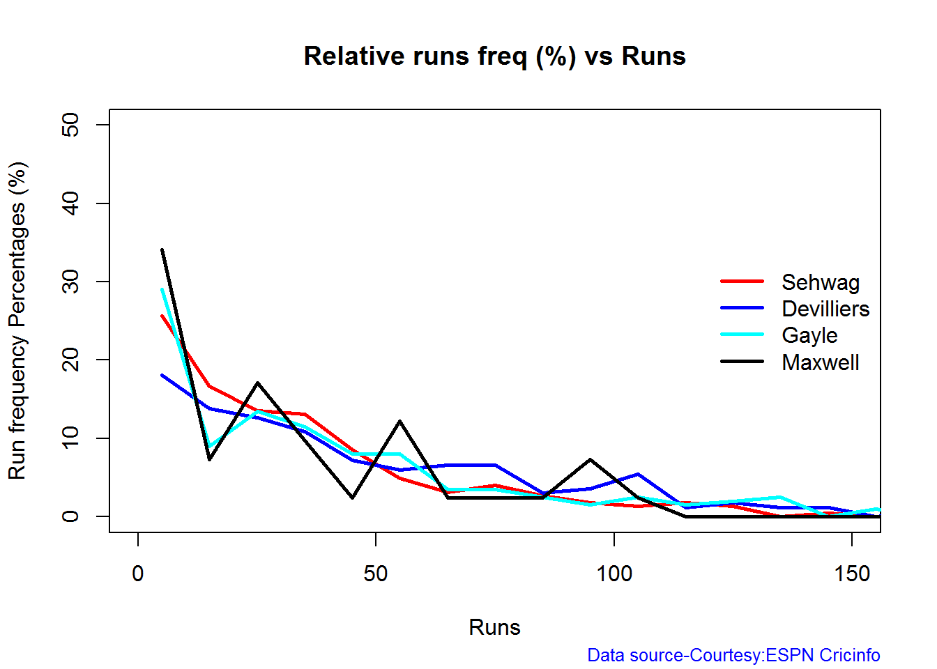
Percentage of 4s,6s in the runs scored
The plot below shows the percentage of runs made by the batsmen by ways of 1s,2s,3s, 4s and 6s. It can be seen that Sehwag has the higheest percent of 4s (33.36%) in his overall runs in ODIs. Maxwell has the highest percentage of 6s (13.36%) in his ODI career. If we take the overall 4s+6s then Sehwag leads with (33.36 +5.95 = 39.31%),followed by Gayle (27.80+10.15=37.95%)
Percent 4’s,6’s in total runs scored
The plot below shows the contrib
frames <- list("./sehwag.csv","./devilliers.csv","gayle.csv","maxwell.csv")
names <- list("Sehwag","Devilliers","Gayle","Maxwell")
runs4s6s <-batsman4s6s(frames,names)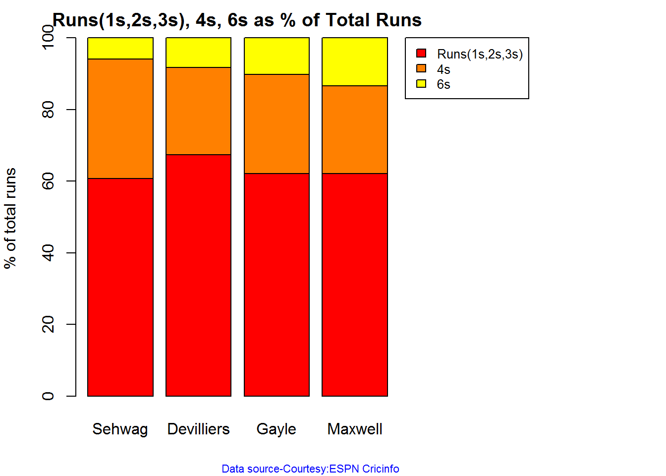
print(runs4s6s)## Sehwag Devilliers Gayle Maxwell
## Runs(1s,2s,3s) 60.69 67.39 62.05 62.11
## 4s 33.36 24.28 27.80 24.53
## 6s 5.95 8.32 10.15 13.36 Runs forecast
The forecast for the batsman is shown below.
par(mfrow=c(2,2))
par(mar=c(4,4,2,2))
batsmanPerfForecast("./sehwag.csv","Sehwag")
batsmanPerfForecast("./devilliers.csv","Devilliers")
batsmanPerfForecast("./gayle.csv","Gayle")
batsmanPerfForecast("./maxwell.csv","Maxwell")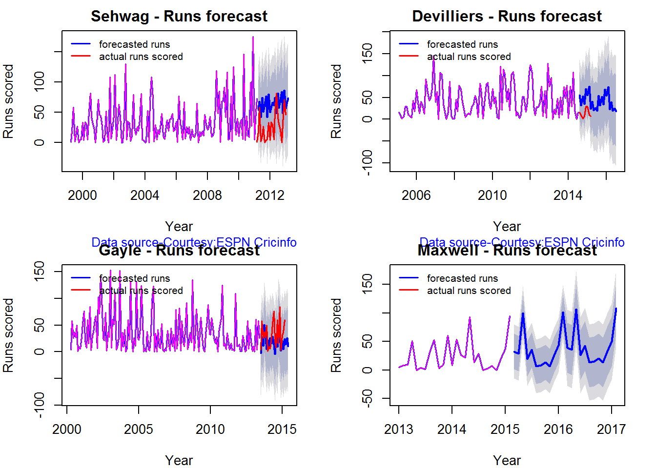
dev.off()## null device
## 13D plot of Runs vs Balls Faced and Minutes at Crease
The plot is a scatter plot of Runs vs Balls faced and Minutes at Crease. A prediction plane is fitted
par(mfrow=c(1,2))
par(mar=c(4,4,2,2))
battingPerf3d("./sehwag.csv","V Sehwag")
battingPerf3d("./devilliers.csv","AB Devilliers")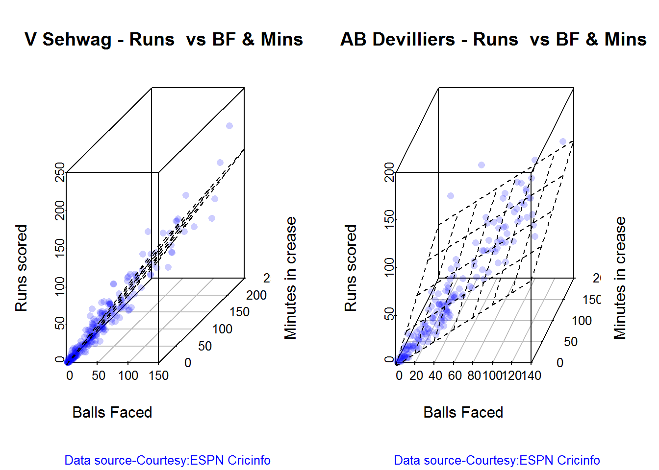
dev.off()## null device
## 1par(mfrow=c(1,2))
par(mar=c(4,4,2,2))
battingPerf3d("./gayle.csv","C Gayle")
battingPerf3d("./maxwell.csv","G Maxwell")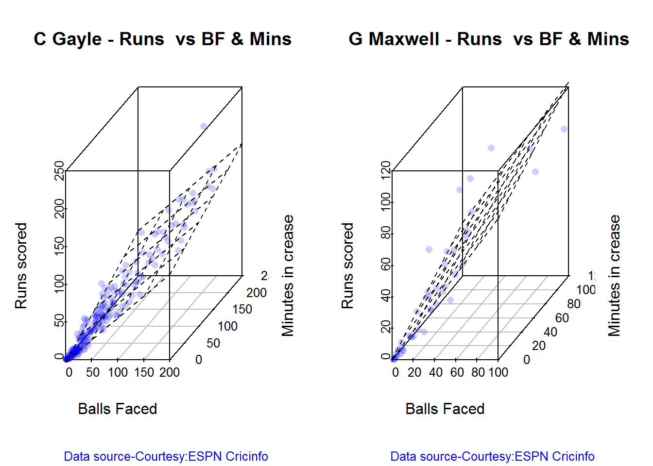
dev.off()## null device
## 1Predicting Runs given Balls Faced and Minutes at Crease
A multi-variate regression plane is fitted between Runs and Balls faced +Minutes at crease.
BF <- seq( 10, 200,length=10)
Mins <- seq(30,220,length=10)
newDF <- data.frame(BF,Mins)
sehwag <- batsmanRunsPredict("./sehwag.csv","Sehwag",newdataframe=newDF)
devilliers <- batsmanRunsPredict("./devilliers.csv","Devilliers",newdataframe=newDF)
gayle <- batsmanRunsPredict("./gayle.csv","Gayle",newdataframe=newDF)
maxwell <- batsmanRunsPredict("./maxwell.csv","Maxwell",newdataframe=newDF)The fitted model is then used to predict the runs that the batsmen will score for a hypotheticial Balls faced and Minutes at crease. It can be seen that Maxwell sets a searing pace in the predicted runs for a given Balls Faced and Minutes at crease followed by Sehwag. But we have to keep in mind that Maxwell has only around 1/5th of the innings of Sehwag (45 to Sehwag’s 245 innings). They are followed by Devilliers and then finally Gayle
batsmen <-cbind(round(sehwag$Runs),round(devilliers$Runs),round(gayle$Runs),round(maxwell$Runs))
colnames(batsmen) <- c("Sehwag","Devilliers","Gayle","Maxwell")
newDF <- data.frame(round(newDF$BF),round(newDF$Mins))
colnames(newDF) <- c("BallsFaced","MinsAtCrease")
predictedRuns <- cbind(newDF,batsmen)
predictedRuns## BallsFaced MinsAtCrease Sehwag Devilliers Gayle Maxwell
## 1 10 30 11 12 11 18
## 2 31 51 33 32 28 43
## 3 52 72 55 52 46 67
## 4 73 93 77 71 63 92
## 5 94 114 100 91 81 117
## 6 116 136 122 111 98 141
## 7 137 157 144 130 116 166
## 8 158 178 167 150 133 191
## 9 179 199 189 170 151 215
## 10 200 220 211 190 168 240Highest runs likelihood
The plots below the runs likelihood of batsman. This uses K-Means It can be seen that Devilliers has almost 27.75% likelihood to make around 90+ runs. Gayle and Sehwag have 34% to make 40+ runs. A. Virender Sehwag
A. Virender Sehwag
batsmanRunsLikelihood("./sehwag.csv","Sehwag")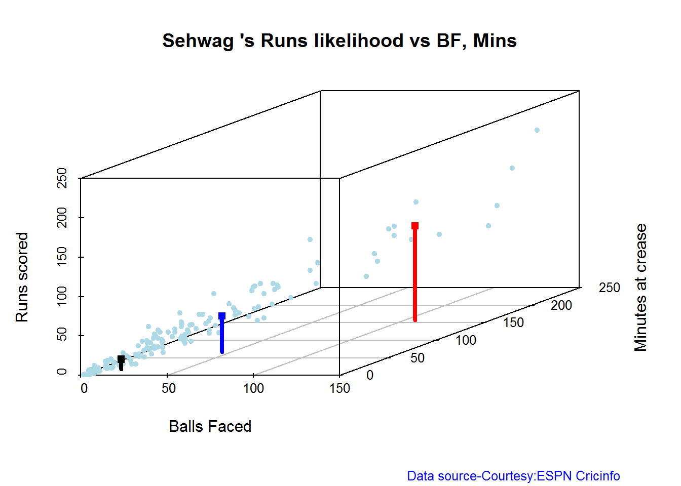
## Summary of Sehwag 's runs scoring likelihood
## **************************************************
##
## There is a 35.22 % likelihood that Sehwag will make 46 Runs in 44 balls over 67 Minutes
## There is a 9.43 % likelihood that Sehwag will make 119 Runs in 106 balls over 158 Minutes
## There is a 55.35 % likelihood that Sehwag will make 12 Runs in 13 balls over 18 MinutesB. AB Devilliers
batsmanRunsLikelihood("./devilliers.csv","Devilliers")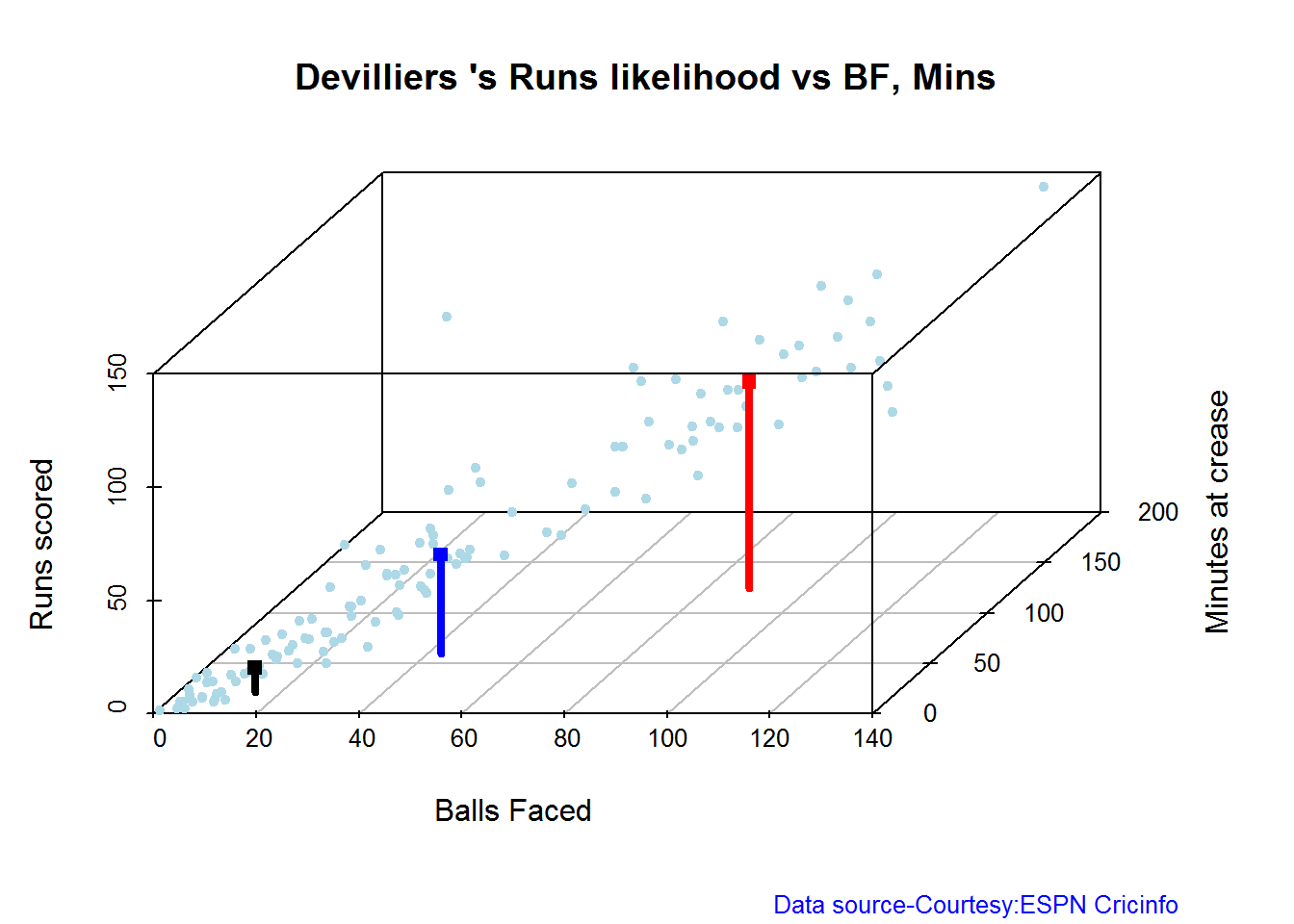
## Summary of Devilliers 's runs scoring likelihood
## **************************************************
##
## There is a 30.65 % likelihood that Devilliers will make 44 Runs in 43 balls over 60 Minutes
## There is a 29.84 % likelihood that Devilliers will make 91 Runs in 88 balls over 124 Minutes
## There is a 39.52 % likelihood that Devilliers will make 11 Runs in 15 balls over 21 MinutesC. Chris Gayle
batsmanRunsLikelihood("./gayle.csv","Gayle")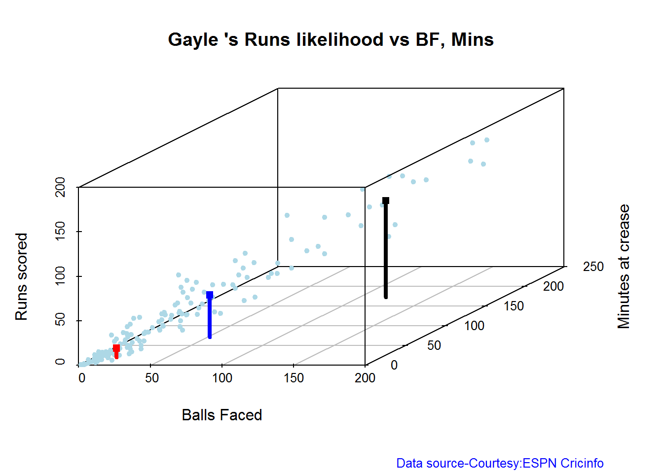
## Summary of Gayle 's runs scoring likelihood
## **************************************************
##
## There is a 32.69 % likelihood that Gayle will make 47 Runs in 51 balls over 72 Minutes
## There is a 54.49 % likelihood that Gayle will make 10 Runs in 15 balls over 20 Minutes
## There is a 12.82 % likelihood that Gayle will make 109 Runs in 119 balls over 172 MinutesD. Glenn Maxwell
batsmanRunsLikelihood("./maxwell.csv","Maxwell")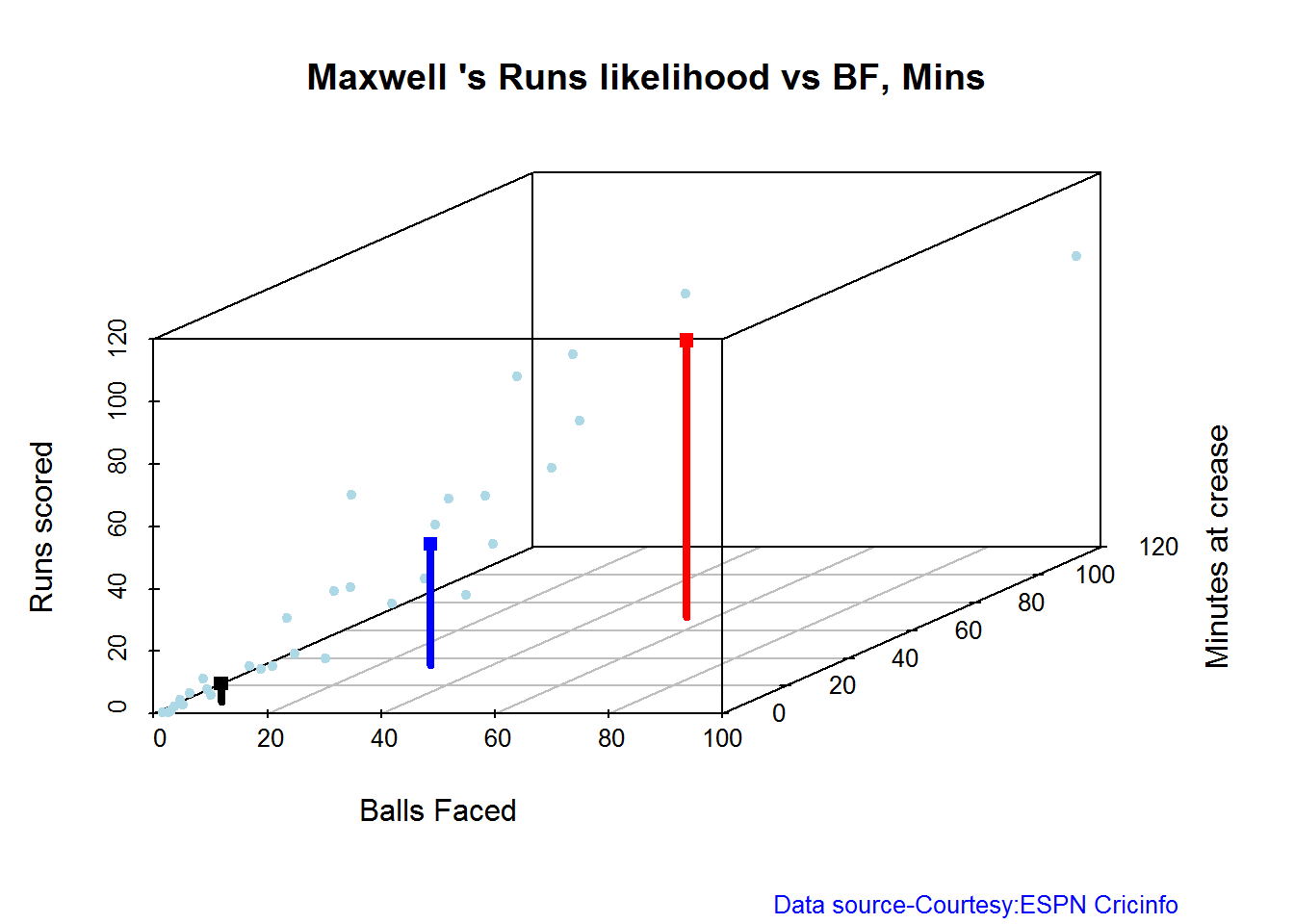
## Summary of Maxwell 's runs scoring likelihood
## **************************************************
##
## There is a 34.38 % likelihood that Maxwell will make 39 Runs in 29 balls over 35 Minutes
## There is a 15.62 % likelihood that Maxwell will make 89 Runs in 55 balls over 69 Minutes
## There is a 50 % likelihood that Maxwell will make 6 Runs in 7 balls over 9 MinutesAverage runs at ground and against opposition
A. Virender Sehwag
par(mfrow=c(1,2))
par(mar=c(4,4,2,2))
batsmanAvgRunsGround("./sehwag.csv","Sehwag")
batsmanAvgRunsOpposition("./sehwag.csv","Sehwag")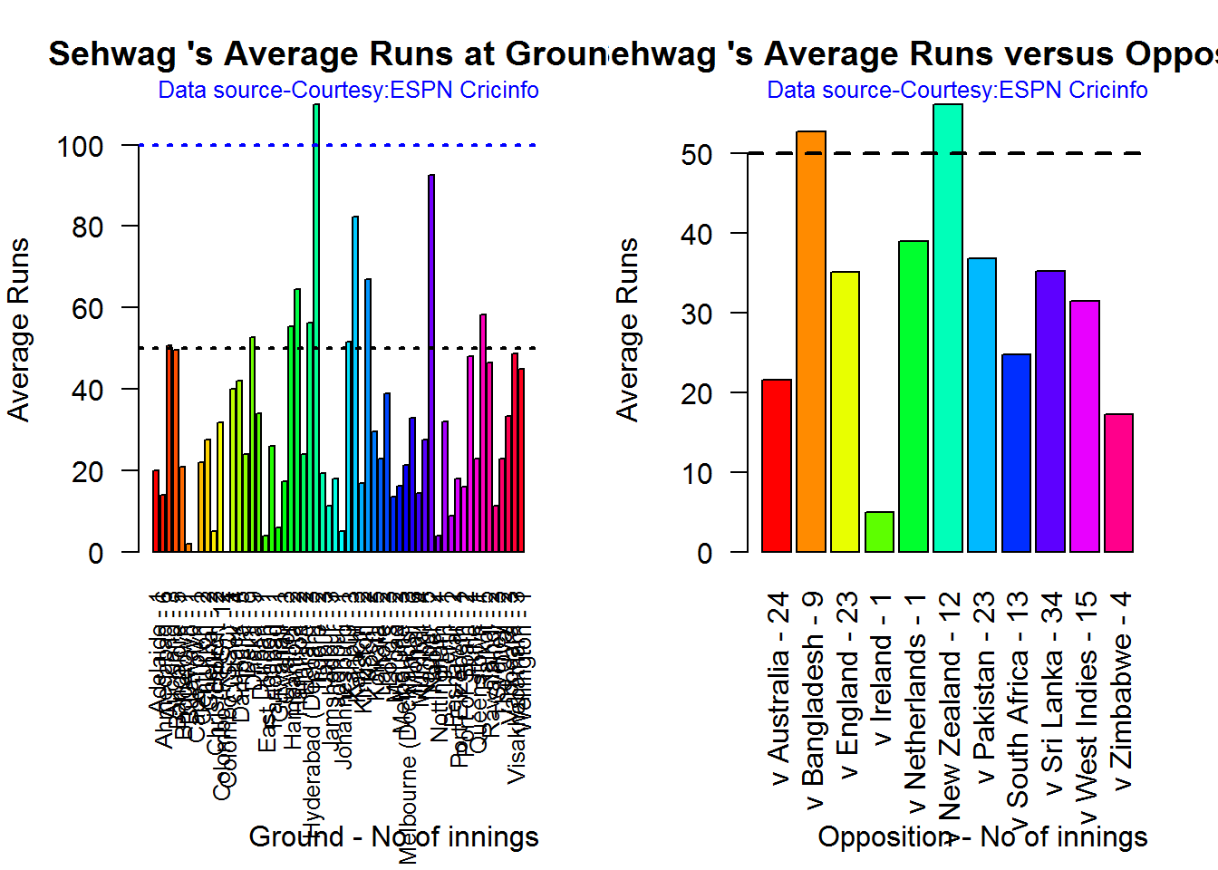
dev.off()## null device
## 1B. AB Devilliers
par(mfrow=c(1,2))
par(mar=c(4,4,2,2))
batsmanAvgRunsGround("./devilliers.csv","Devilliers")
batsmanAvgRunsOpposition("./devilliers.csv","Devilliers")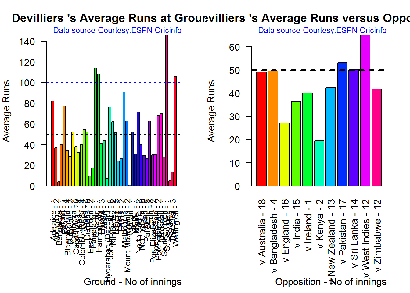
dev.off()## null device
## 1C. Chris Gayle
par(mfrow=c(1,2))
par(mar=c(4,4,2,2))
batsmanAvgRunsGround("./gayle.csv","Gayle")
batsmanAvgRunsOpposition("./gayle.csv","Gayle")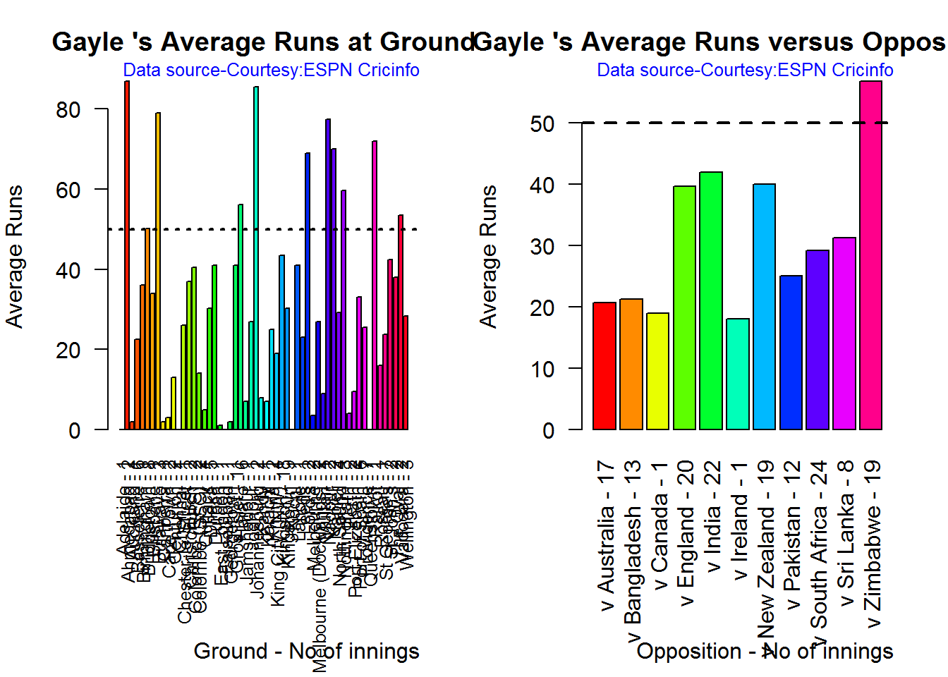
dev.off()## null device
## 1D. Glenn Maxwell
par(mfrow=c(1,2))
par(mar=c(4,4,2,2))
batsmanAvgRunsGround("./maxwell.csv","Maxwell")
batsmanAvgRunsOpposition("./maxwell.csv","Maxwell")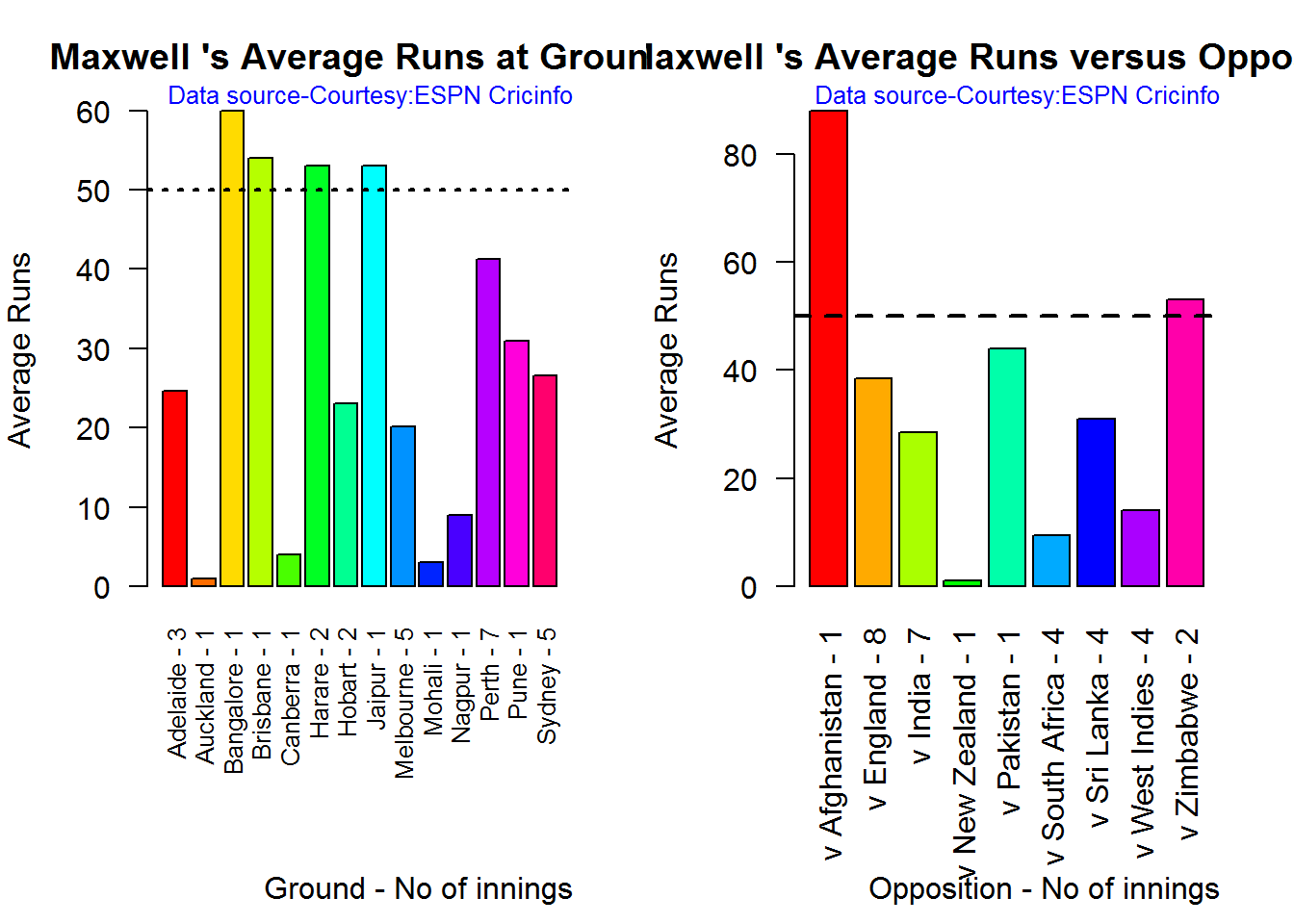
dev.off()## null device
## 1Moving Average of runs over career
The moving average for the 4 batsmen indicate the following
1. The moving average of Devilliers and Maxwell is on the way up.
2. Sehwag shows a slight downward trend from his 2nd peak in 2011
3. Gayle maintains a consistent 45 runs for the last few years
par(mfrow=c(2,2))
par(mar=c(4,4,2,2))
batsmanMovingAverage("./sehwag.csv","Sehwag")
batsmanMovingAverage("./devilliers.csv","Devilliers")
batsmanMovingAverage("./gayle.csv","Gayle")
batsmanMovingAverage("./maxwell.csv","Maxwell")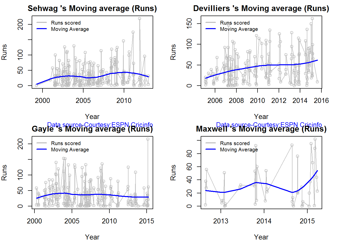
dev.off()## null device
## 1Check batsmen in-form, out-of-form
- Maxwell, Devilliers, Sehwag are in-form. This is also evident from the moving average plot
- Gayle is out-of-form
checkBatsmanInForm("./sehwag.csv","Sehwag")## *******************************************************************************************
##
## Population size: 143 Mean of population: 33.76
## Sample size: 16 Mean of sample: 37.44 SD of sample: 55.15
##
## Null hypothesis H0 : Sehwag 's sample average is within 95% confidence interval
## of population average
## Alternative hypothesis Ha : Sehwag 's sample average is below the 95% confidence
## interval of population average
##
## [1] "Sehwag 's Form Status: In-Form because the p value: 0.603525 is greater than alpha= 0.05"
## *******************************************************************************************checkBatsmanInForm("./devilliers.csv","Devilliers")## *******************************************************************************************
##
## Population size: 111 Mean of population: 43.5
## Sample size: 13 Mean of sample: 57.62 SD of sample: 40.69
##
## Null hypothesis H0 : Devilliers 's sample average is within 95% confidence interval
## of population average
## Alternative hypothesis Ha : Devilliers 's sample average is below the 95% confidence
## interval of population average
##
## [1] "Devilliers 's Form Status: In-Form because the p value: 0.883541 is greater than alpha= 0.05"
## *******************************************************************************************checkBatsmanInForm("./gayle.csv","Gayle")## *******************************************************************************************
##
## Population size: 140 Mean of population: 37.1
## Sample size: 16 Mean of sample: 17.25 SD of sample: 20.25
##
## Null hypothesis H0 : Gayle 's sample average is within 95% confidence interval
## of population average
## Alternative hypothesis Ha : Gayle 's sample average is below the 95% confidence
## interval of population average
##
## [1] "Gayle 's Form Status: Out-of-Form because the p value: 0.000609 is less than alpha= 0.05"
## *******************************************************************************************checkBatsmanInForm("./maxwell.csv","Maxwell")## *******************************************************************************************
##
## Population size: 28 Mean of population: 25.25
## Sample size: 4 Mean of sample: 64.25 SD of sample: 36.97
##
## Null hypothesis H0 : Maxwell 's sample average is within 95% confidence interval
## of population average
## Alternative hypothesis Ha : Maxwell 's sample average is below the 95% confidence
## interval of population average
##
## [1] "Maxwell 's Form Status: In-Form because the p value: 0.948744 is greater than alpha= 0.05"
## *******************************************************************************************Analysis of bowlers
- Mitchell Johnson (Aus) – Innings-150, Wickets – 239, Econ Rate : 4.83
- Lasith Malinga (SL)- Innings-182, Wickets – 287, Econ Rate : 5.26
- Dale Steyn (SA)- Innings-103, Wickets – 162, Econ Rate : 4.81
- Tim Southee (NZ)- Innings-96, Wickets – 135, Econ Rate : 5.33
Malinga has the highest number of innings and wickets followed closely by Mitchell. Steyn and Southee have relatively fewer innings.
To get the bowler’s data use
malinga <- getPlayerDataOD(49758,dir=".",file="malinga.csv",type="bowling")Wicket Frequency percentage
This plot gives the percentage of wickets for each wickets (1,2,3…etc)
par(mfrow=c(1,4))
par(mar=c(4,4,2,2))
bowlerWktsFreqPercent("./mitchell.csv","J Mitchell")
bowlerWktsFreqPercent("./malinga.csv","Malinga")
bowlerWktsFreqPercent("./steyn.csv","Steyn")
bowlerWktsFreqPercent("./southee.csv","southee")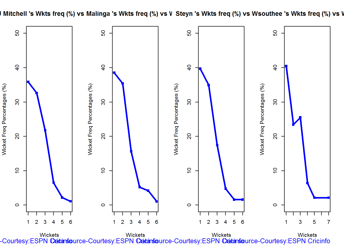
dev.off()## null device
## 1Wickets Runs plot
The plot below gives a boxplot of the runs ranges for each of the wickets taken by the bowlers. M Johnson and Steyn are more economical than Malinga and Southee corroborating the figures above
par(mfrow=c(1,4))
par(mar=c(4,4,2,2))
bowlerWktsRunsPlot("./mitchell.csv","J Mitchell")
bowlerWktsRunsPlot("./malinga.csv","Malinga")
bowlerWktsRunsPlot("./steyn.csv","Steyn")
bowlerWktsRunsPlot("./southee.csv","southee")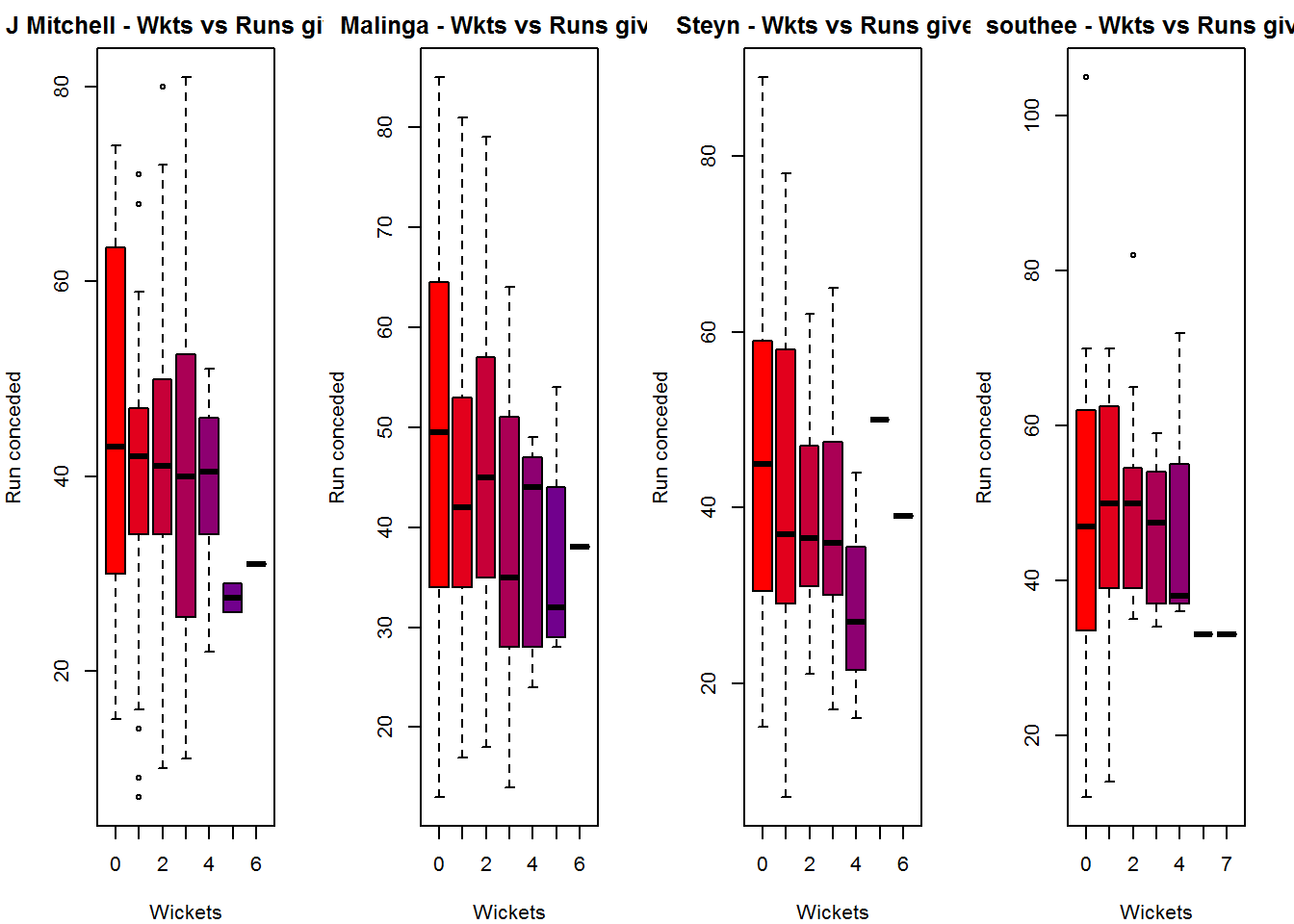
dev.off()## null device
## 1Average wickets in different grounds and opposition
A. Mitchell Johnson
par(mfrow=c(1,2))
par(mar=c(4,4,2,2))
bowlerAvgWktsGround("./mitchell.csv","J Mitchell")
bowlerAvgWktsOpposition("./mitchell.csv","J Mitchell")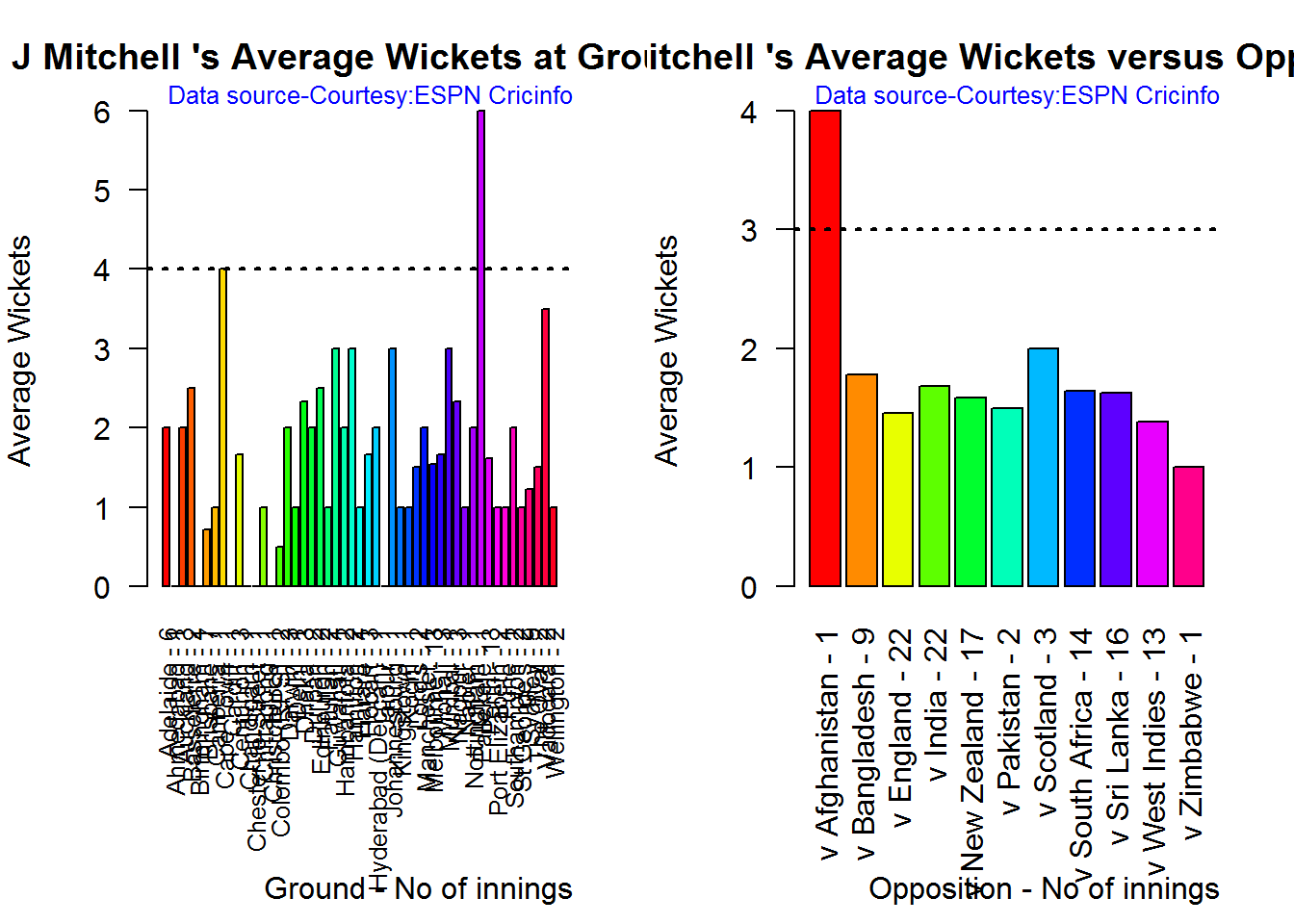
dev.off()## null device
## 1B. Lasith Malinga
par(mfrow=c(1,2))
par(mar=c(4,4,2,2))
bowlerAvgWktsGround("./malinga.csv","Malinga")
bowlerAvgWktsOpposition("./malinga.csv","Malinga")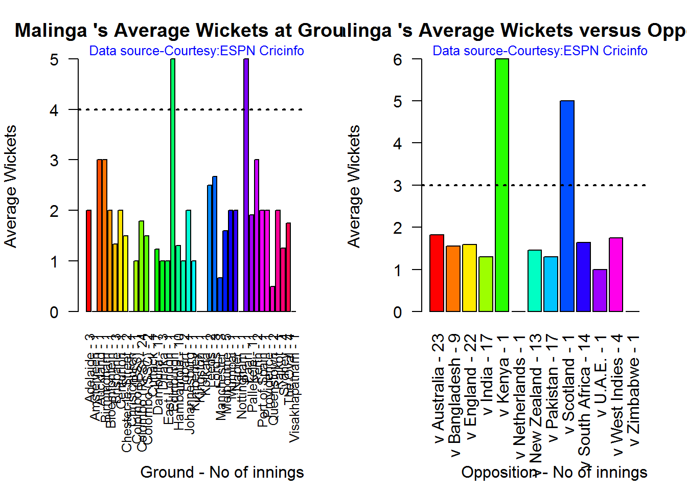
dev.off()## null device
## 1C. Dale Steyn
par(mfrow=c(1,2))
par(mar=c(4,4,2,2))
bowlerAvgWktsGround("./steyn.csv","Steyn")
bowlerAvgWktsOpposition("./steyn.csv","Steyn")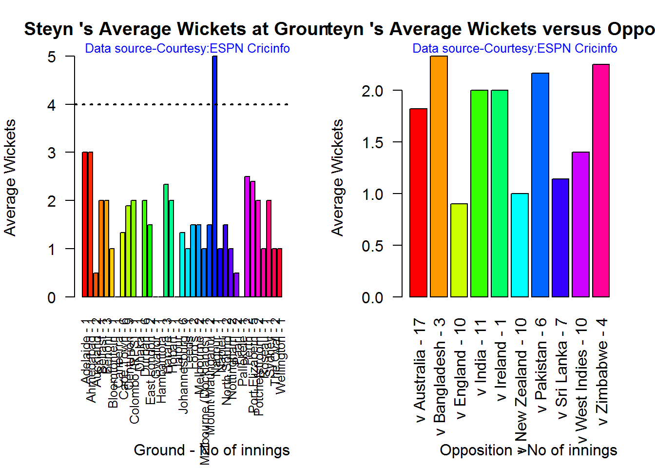
dev.off()## null device
## 1D. Tim Southee
par(mfrow=c(1,2))
par(mar=c(4,4,2,2))
bowlerAvgWktsGround("./southee.csv","southee")
bowlerAvgWktsOpposition("./southee.csv","southee")
dev.off()## null device
## 1Relative bowling performance
The plot below shows that Mitchell Johnson and Southee have more wickets in 3-4 wickets range while Steyn and Malinga in 1-2 wicket range
frames <- list("./mitchell.csv","./malinga.csv","steyn.csv","southee.csv")
names <- list("M Johnson","Malinga","Steyn","Southee")
relativeBowlingPerf(frames,names)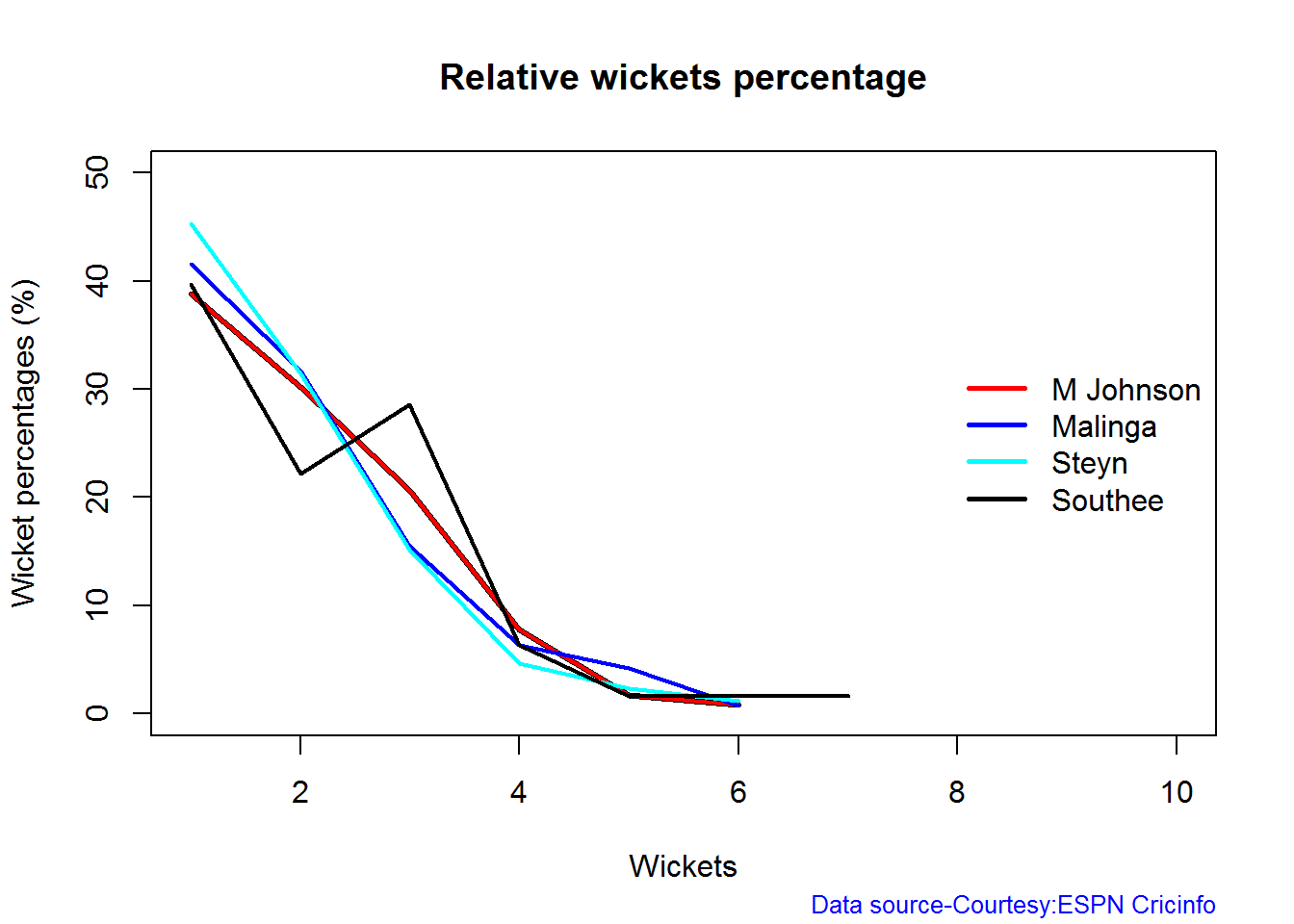
Relative Economy Rate against wickets taken
Steyn had the best economy rate followed by M Johnson. Malinga and Southee have a poorer economy rate
frames <- list("./mitchell.csv","./malinga.csv","steyn.csv","southee.csv")
names <- list("M Johnson","Malinga","Steyn","Southee")
relativeBowlingERODTT(frames,names)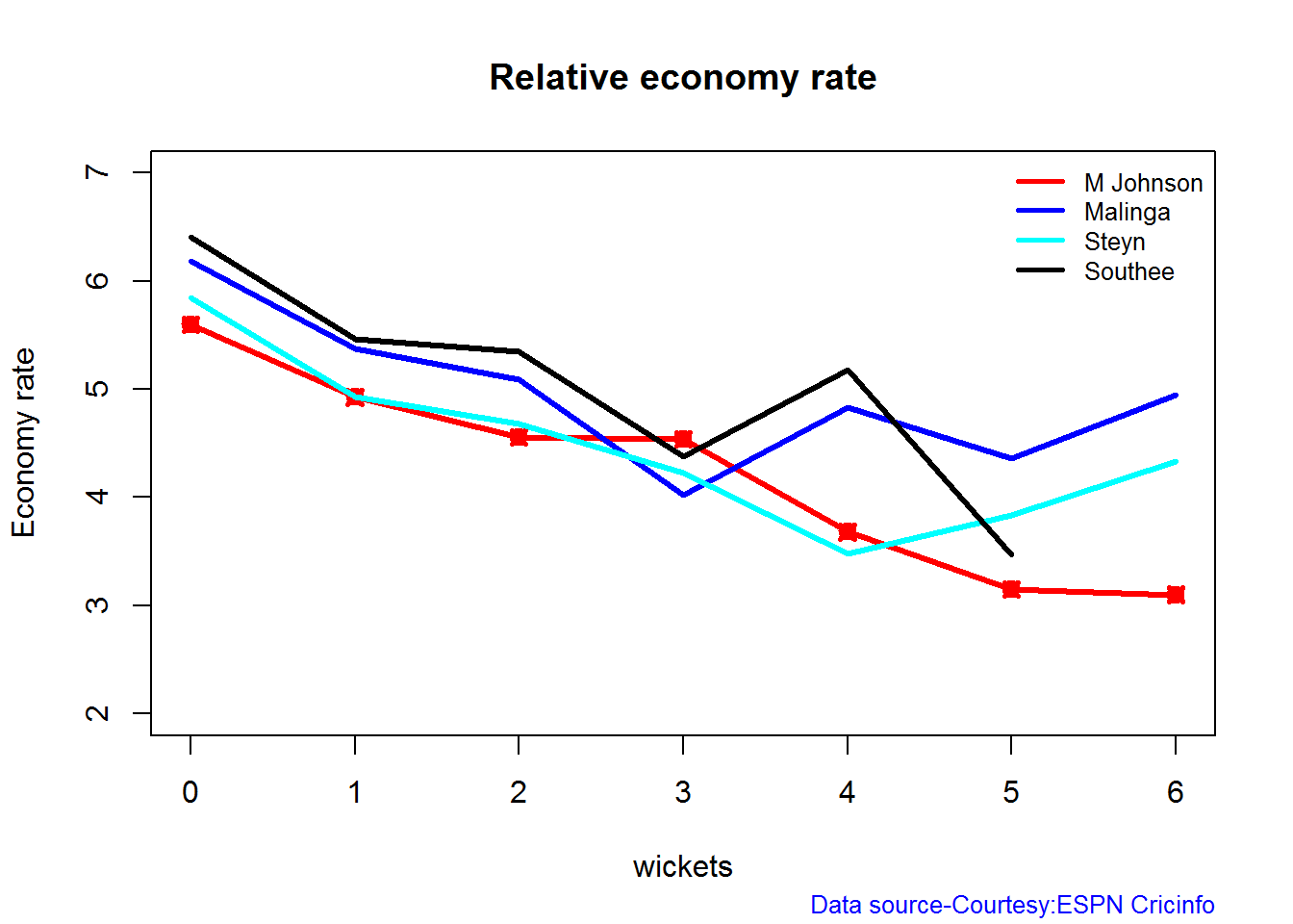
Moving average of wickets over career
Johnson and Steyn career vs wicket graph is on the up-swing. Southee is maintaining a reasonable record while Malinga shows a decline in ODI performance
par(mfrow=c(2,2))
par(mar=c(4,4,2,2))
bowlerMovingAverage("./mitchell.csv","M Johnson")
bowlerMovingAverage("./malinga.csv","Malinga")
bowlerMovingAverage("./steyn.csv","Steyn")
bowlerMovingAverage("./southee.csv","Southee")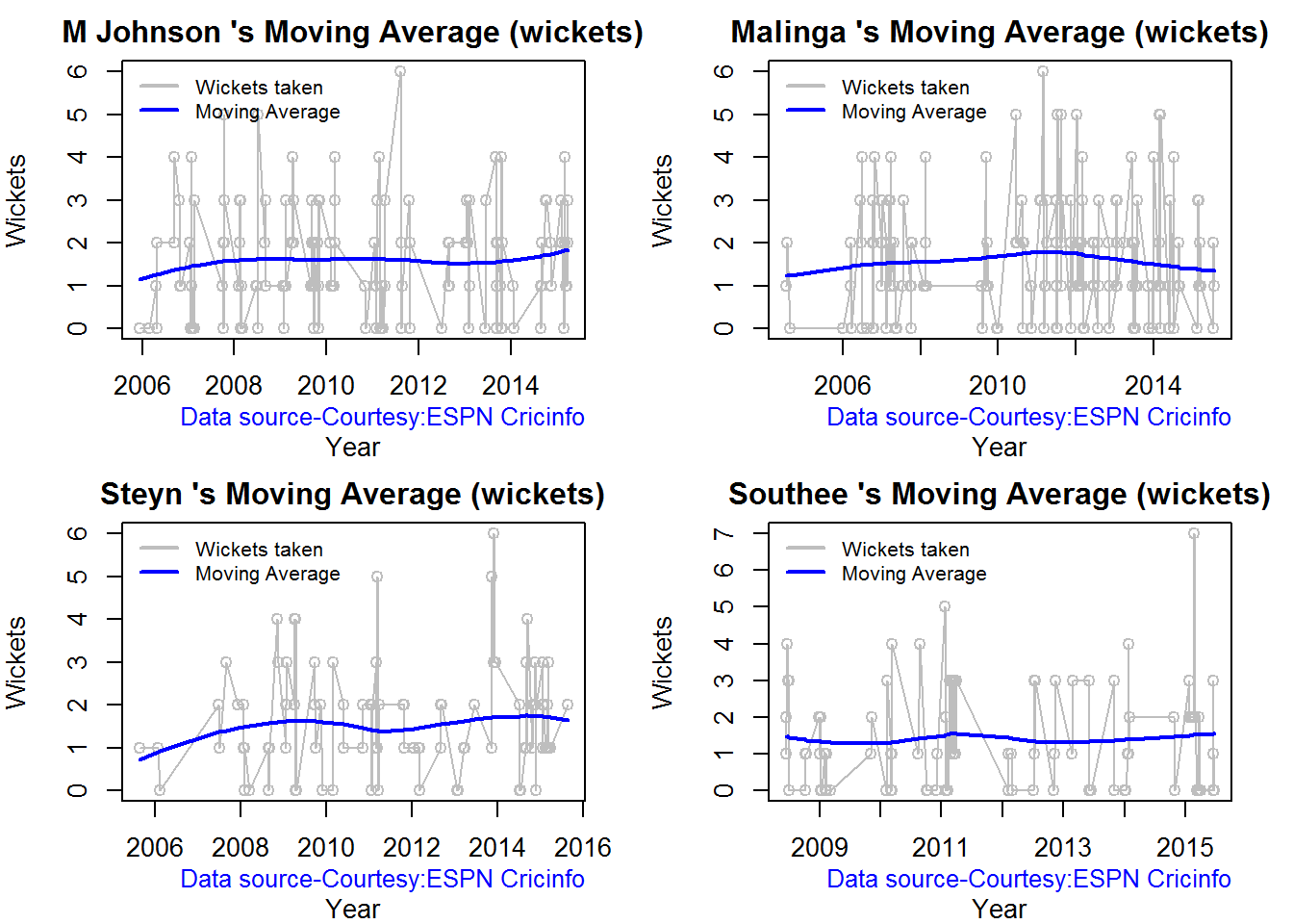
dev.off()## null device
## 1Wickets forecast
par(mfrow=c(2,2))
par(mar=c(4,4,2,2))
bowlerPerfForecast("./mitchell.csv","M Johnson")
bowlerPerfForecast("./malinga.csv","Malinga")
bowlerPerfForecast("./steyn.csv","Steyn")
bowlerPerfForecast("./southee.csv","southee")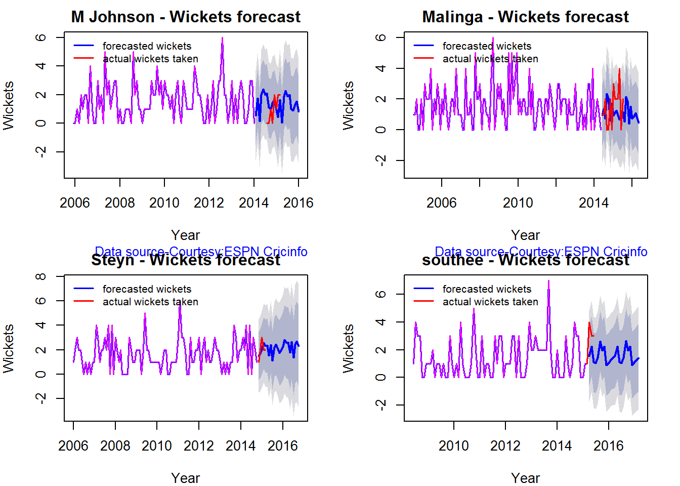
dev.off()## null device
## 1Check bowler in-form, out-of-form
All the bowlers are shown to be still in-form
checkBowlerInForm("./mitchell.csv","J Mitchell")## *******************************************************************************************
##
## Population size: 135 Mean of population: 1.55
## Sample size: 15 Mean of sample: 2 SD of sample: 1.07
##
## Null hypothesis H0 : J Mitchell 's sample average is within 95% confidence interval
## of population average
## Alternative hypothesis Ha : J Mitchell 's sample average is below the 95% confidence
## interval of population average
##
## [1] "J Mitchell 's Form Status: In-Form because the p value: 0.937917 is greater than alpha= 0.05"
## *******************************************************************************************checkBowlerInForm("./malinga.csv","Malinga")## *******************************************************************************************
##
## Population size: 163 Mean of population: 1.58
## Sample size: 19 Mean of sample: 1.58 SD of sample: 1.22
##
## Null hypothesis H0 : Malinga 's sample average is within 95% confidence interval
## of population average
## Alternative hypothesis Ha : Malinga 's sample average is below the 95% confidence
## interval of population average
##
## [1] "Malinga 's Form Status: In-Form because the p value: 0.5 is greater than alpha= 0.05"
## *******************************************************************************************checkBowlerInForm("./steyn.csv","Steyn")## *******************************************************************************************
##
## Population size: 93 Mean of population: 1.59
## Sample size: 11 Mean of sample: 1.45 SD of sample: 0.69
##
## Null hypothesis H0 : Steyn 's sample average is within 95% confidence interval
## of population average
## Alternative hypothesis Ha : Steyn 's sample average is below the 95% confidence
## interval of population average
##
## [1] "Steyn 's Form Status: In-Form because the p value: 0.257438 is greater than alpha= 0.05"
## *******************************************************************************************checkBowlerInForm("./southee.csv","southee")## *******************************************************************************************
##
## Population size: 86 Mean of population: 1.48
## Sample size: 10 Mean of sample: 0.8 SD of sample: 1.14
##
## Null hypothesis H0 : southee 's sample average is within 95% confidence interval
## of population average
## Alternative hypothesis Ha : southee 's sample average is below the 95% confidence
## interval of population average
##
## [1] "southee 's Form Status: Out-of-Form because the p value: 0.044302 is less than alpha= 0.05"
## **********************************************************************************************************
Key findings
Here are some key conclusions ODI batsmen
- AB Devilliers has high frequency of runs in the 60-120 range and the highest average
- Sehwag has the most number of innings and good strike rate
- Maxwell has the best strike rate but it should be kept in mind that he has 1/5 of the innings of Sehwag. We need to see how he progress further
- Sehwag has the highest percentage of 4s in the runs scored, while Maxwell has the most 6s
- For a hypothetical Balls Faced and Minutes at creases Maxwell will score the most runs followed by Sehwag
- The moving average of indicates that the best is yet to come for Devilliers and Maxwell. Sehwag has a few more years in him while Gayle shows a decline in ODI performance and an out of form is indicated.
ODI bowlers
- Malinga has the highest played the highest innings and also has the highest wickets though he has poor economy rate
- M Johnson is the most effective in the 3-4 wicket range followed by Southee
- M Johnson and Steyn has the best overall economy rate followed by Malinga and Steyn 4 M Johnson and Steyn’s career is on the up-swing,Southee maintains a steady consistent performance, while Malinga shows a downward trend
Hasta la vista! I’ll be back!
Watch this space!
Also see my other posts in R
- Introducing cricketr! : An R package to analyze performances of cricketers
- cricketr digs the Ashes!
- A peek into literacy in India: Statistical Learning with R
- A crime map of India in R – Crimes against women
- Analyzing cricket’s batting legends – Through the mirage with R
- Mirror, mirror . the best batsman of them all?
You may also like
- A closer look at “Robot Horse on a Trot” in Android
- What’s up Watson? Using IBM Watson’s QAAPI with Bluemix, NodeExpress – Part 1
- Bend it like Bluemix, MongoDB with autoscaling – Part 2
- Informed choices through Machine Learning : Analyzing Kohli, Tendulkar and Dravid
- TWS-4: Gossip protocol: Epidemics and rumors to the rescue
- Deblurring with OpenCV:Weiner filter reloadedhttp://www.r-bloggers.com/cricketr-plays-the-odis/
Share:

cricketr digs the Ashes!
Published in R bloggers: cricketr digs the Ashes
Introduction
In some circles the Ashes is considered the ‘mother of all cricketing battles’. But, being a staunch supporter of all things Indian, cricket or otherwise, I have to say that the Ashes pales in comparison against a India-Pakistan match. After all, what are a few frowns and raised eyebrows at the Ashes in comparison to the seething emotions and reckless exuberance of Indian fans.
Anyway, the Ashes are an interesting duel and I have decided to do some cricketing analysis using my R package cricketr. For this analysis I have chosen the top 2 batsman and top 2 bowlers from both the Australian and English sides.
Batsmen
- Steven Smith (Aus) – Innings – 58 , Ave: 58.52, Strike Rate: 55.90
- David Warner (Aus) – Innings – 76, Ave: 46.86, Strike Rate: 73.88
- Alistair Cook (Eng) – Innings – 208 , Ave: 46.62, Strike Rate: 46.33
- J E Root (Eng) – Innings – 53, Ave: 54.02, Strike Rate: 51.30
Bowlers
- Mitchell Johnson (Aus) – Innings-131, Wickets – 299, Econ Rate : 3.28
- Peter Siddle (Aus) – Innings – 104 , Wickets- 192, Econ Rate : 2.95
- James Anderson (Eng) – Innings – 199 , Wickets- 406, Econ Rate : 3.05
- Stuart Broad (Eng) – Innings – 148 , Wickets- 296, Econ Rate : 3.08
It is my opinion if any 2 of the 4 in either team click then they will be able to swing the match in favor of their team.
I have interspersed the plots with a few comments. Feel free to draw your conclusions!
If you are passionate about cricket, and love analyzing cricket performances, then check out my racy book on cricket ‘Cricket analytics with cricketr and cricpy – Analytics harmony with R & Python’! This book discusses and shows how to use my R package ‘cricketr’ and my Python package ‘cricpy’ to analyze batsmen and bowlers in all formats of the game (Test, ODI and T20). The paperback is available on Amazon at $21.99 and the kindle version at $9.99/Rs 449/-. A must read for any cricket lover! Check it out!!
You can download the latest PDF version of the book at ‘Cricket analytics with cricketr and cricpy: Analytics harmony with R and Python-6th edition‘
cks), and $4.99/Rs 320 and $6.99/Rs448 respectively
Important note 1: The latest release of ‘cricketr’ now includes the ability to analyze performances of teams now!! See Cricketr adds team analytics to its repertoire!!!
Important note 2 : Cricketr can now do a more fine-grained analysis of players, see Cricketr learns new tricks : Performs fine-grained analysis of players
Important note 3: Do check out the python avatar of cricketr, ‘cricpy’ in my post ‘Introducing cricpy:A python package to analyze performances of cricketers”
The analysis is included below. Note: This post has also been hosted at Rpubs as cricketr digs the Ashes!
You can also download this analysis as a PDF file from cricketr digs the Ashes!
Do check out my interactive Shiny app implementation using the cricketr package – Sixer – R package cricketr’s new Shiny avatar
Note: If you would like to do a similar analysis for a different set of batsman and bowlers, you can clone/download my skeleton cricketr template from Github (which is the R Markdown file I have used for the analysis below). You will only need to make appropriate changes for the players you are interested in. Just a familiarity with R and R Markdown only is needed.
Important note: Do check out my other posts using cricketr at cricketr-posts
The package can be installed directly from CRAN
if (!require("cricketr")){
install.packages("cricketr",lib = "c:/test")
}
library(cricketr)or from Github
library(devtools)
install_github("tvganesh/cricketr")
library(cricketr)Analyses of Batsmen
The following plots gives the analysis of the 2 Australian and 2 English batsmen. It must be kept in mind that Cooks has more innings than all the rest put together. Smith has the best average, and Warner has the best strike rate
Box Histogram Plot
This plot shows a combined boxplot of the Runs ranges and a histogram of the Runs Frequency
batsmanPerfBoxHist("./smith.csv","S Smith")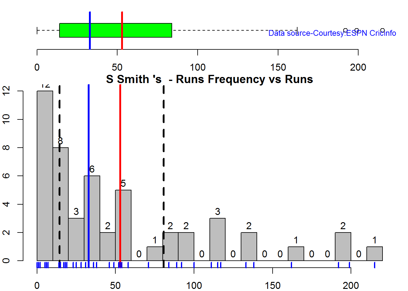
batsmanPerfBoxHist("./warner.csv","D Warner")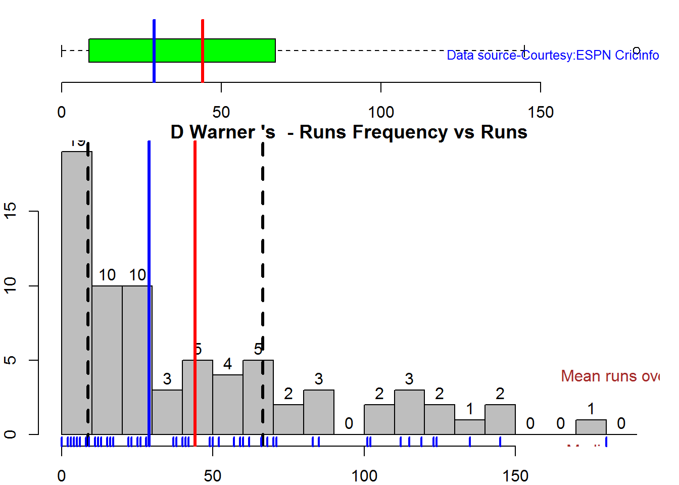
batsmanPerfBoxHist("./cook.csv","A Cook")
batsmanPerfBoxHist("./root.csv","JE Root")
Plot os 4s, 6s and the type of dismissals
A. Steven Smith
par(mfrow=c(1,3))
par(mar=c(4,4,2,2))
batsman4s("./smith.csv","S Smith")
batsman6s("./smith.csv","S Smith")
batsmanDismissals("./smith.csv","S Smith")
dev.off()## null device
## 1B. David Warner
par(mfrow=c(1,3))
par(mar=c(4,4,2,2))
batsman4s("./warner.csv","D Warner")
batsman6s("./warner.csv","D Warner")
batsmanDismissals("./warner.csv","D Warner")
dev.off()## null device
## 1C. Alistair Cook
par(mfrow=c(1,3))
par(mar=c(4,4,2,2))
batsman4s("./cook.csv","A Cook")
batsman6s("./cook.csv","A Cook")
batsmanDismissals("./cook.csv","A Cook")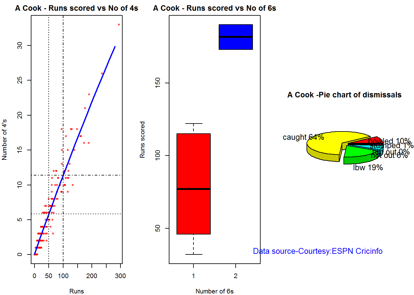
dev.off()## null device
## 1D. J E Root
par(mfrow=c(1,3))
par(mar=c(4,4,2,2))
batsman4s("./root.csv","JE Root")
batsman6s("./root.csv","JE Root")
batsmanDismissals("./root.csv","JE Root")
dev.off()## null device
## 1Relative Mean Strike Rate
In this first plot I plot the Mean Strike Rate of the batsmen. It can be Warner’s has the best strike rate (hit outside the plot!) followed by Smith in the range 20-100. Root has a good strike rate above hundred runs. Cook maintains a good strike rate.
par(mar=c(4,4,2,2))
frames <- list("./smith.csv","./warner.csv","cook.csv","root.csv")
names <- list("Smith","Warner","Cook","Root")
relativeBatsmanSR(frames,names)
Relative Runs Frequency Percentage
The plot below show the percentage contribution in each 10 runs bucket over the entire career.It can be seen that Smith pops up above the rest with remarkable regularity.COok is consistent over the entire range.
frames <- list("./smith.csv","./warner.csv","cook.csv","root.csv")
names <- list("Smith","Warner","Cook","Root")
relativeRunsFreqPerf(frames,names)
Moving Average of runs over career
The moving average for the 4 batsmen indicate the following 1. S Smith is the most promising. There is a marked spike in Performance. Cook maintains a steady pace and is consistent over the years averaging 50 over the years.
par(mfrow=c(2,2))
par(mar=c(4,4,2,2))
batsmanMovingAverage("./smith.csv","S Smith")
batsmanMovingAverage("./warner.csv","D Warner")
batsmanMovingAverage("./cook.csv","A Cook")
batsmanMovingAverage("./root.csv","JE Root")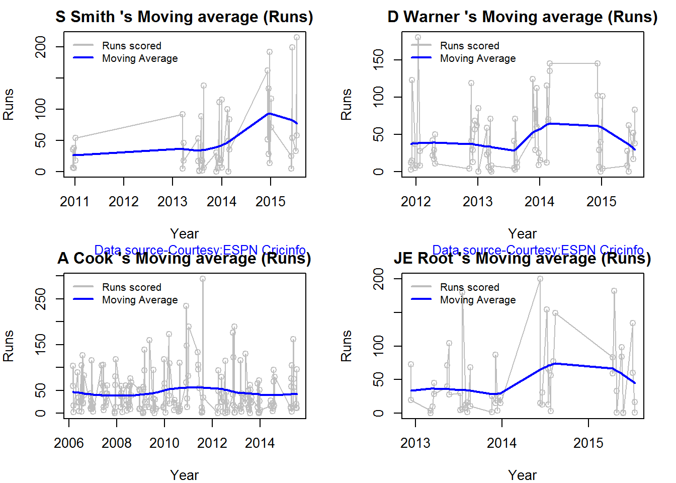
dev.off()## null device
## 1Runs forecast
The forecast for the batsman is shown below. As before Cooks’s performance is really consistent across the years and the forecast is good for the years ahead. In Cook’s case it can be seen that the forecasted and actual runs are reasonably accurate
par(mfrow=c(2,2))
par(mar=c(4,4,2,2))
batsmanPerfForecast("./smith.csv","S Smith")
batsmanPerfForecast("./warner.csv","D Warner")
batsmanPerfForecast("./cook.csv","A Cook")## Warning in HoltWinters(ts.train): optimization difficulties: ERROR:
## ABNORMAL_TERMINATION_IN_LNSRCHbatsmanPerfForecast("./root.csv","JE Root")
dev.off()## null device
## 13D plot of Runs vs Balls Faced and Minutes at Crease
The plot is a scatter plot of Runs vs Balls faced and Minutes at Crease. A prediction plane is fitted
par(mfrow=c(1,2))
par(mar=c(4,4,2,2))
battingPerf3d("./smith.csv","S Smith")
battingPerf3d("./warner.csv","D Warner")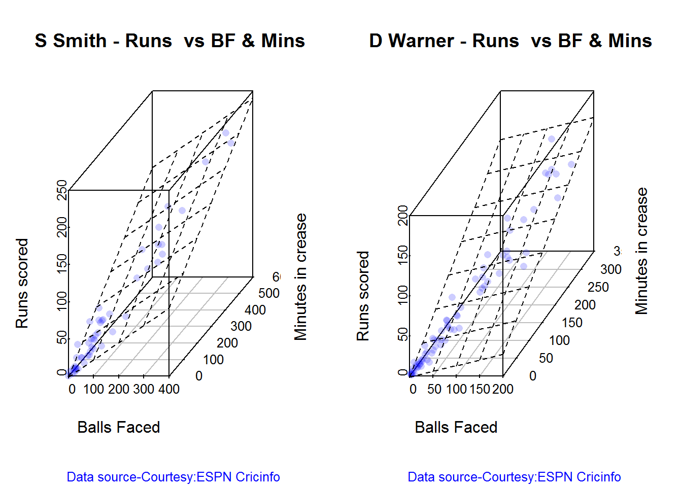
par(mfrow=c(1,2))
par(mar=c(4,4,2,2))
battingPerf3d("./cook.csv","A Cook")
battingPerf3d("./root.csv","JE Root")
dev.off()## null device
## 1Predicting Runs given Balls Faced and Minutes at Crease
A multi-variate regression plane is fitted between Runs and Balls faced +Minutes at crease.
BF <- seq( 10, 400,length=15)
Mins <- seq(30,600,length=15)
newDF <- data.frame(BF,Mins)
smith <- batsmanRunsPredict("./smith.csv","S Smith",newdataframe=newDF)
warner <- batsmanRunsPredict("./warner.csv","D Warner",newdataframe=newDF)
cook <- batsmanRunsPredict("./cook.csv","A Cook",newdataframe=newDF)
root <- batsmanRunsPredict("./root.csv","JE Root",newdataframe=newDF)The fitted model is then used to predict the runs that the batsmen will score for a given Balls faced and Minutes at crease. It can be seen that Warner sets a searing pace in the predicted runs for a given Balls Faced and Minutes at crease while Smith and Root are neck to neck in the predicted runs
batsmen <-cbind(round(smith$Runs),round(warner$Runs),round(cook$Runs),round(root$Runs))
colnames(batsmen) <- c("Smith","Warner","Cook","Root")
newDF <- data.frame(round(newDF$BF),round(newDF$Mins))
colnames(newDF) <- c("BallsFaced","MinsAtCrease")
predictedRuns <- cbind(newDF,batsmen)
predictedRuns## BallsFaced MinsAtCrease Smith Warner Cook Root
## 1 10 30 9 12 6 9
## 2 38 71 25 33 20 25
## 3 66 111 42 53 33 42
## 4 94 152 58 73 47 59
## 5 121 193 75 93 60 75
## 6 149 234 91 114 74 92
## 7 177 274 108 134 88 109
## 8 205 315 124 154 101 125
## 9 233 356 141 174 115 142
## 10 261 396 158 195 128 159
## 11 289 437 174 215 142 175
## 12 316 478 191 235 155 192
## 13 344 519 207 255 169 208
## 14 372 559 224 276 182 225
## 15 400 600 240 296 196 242
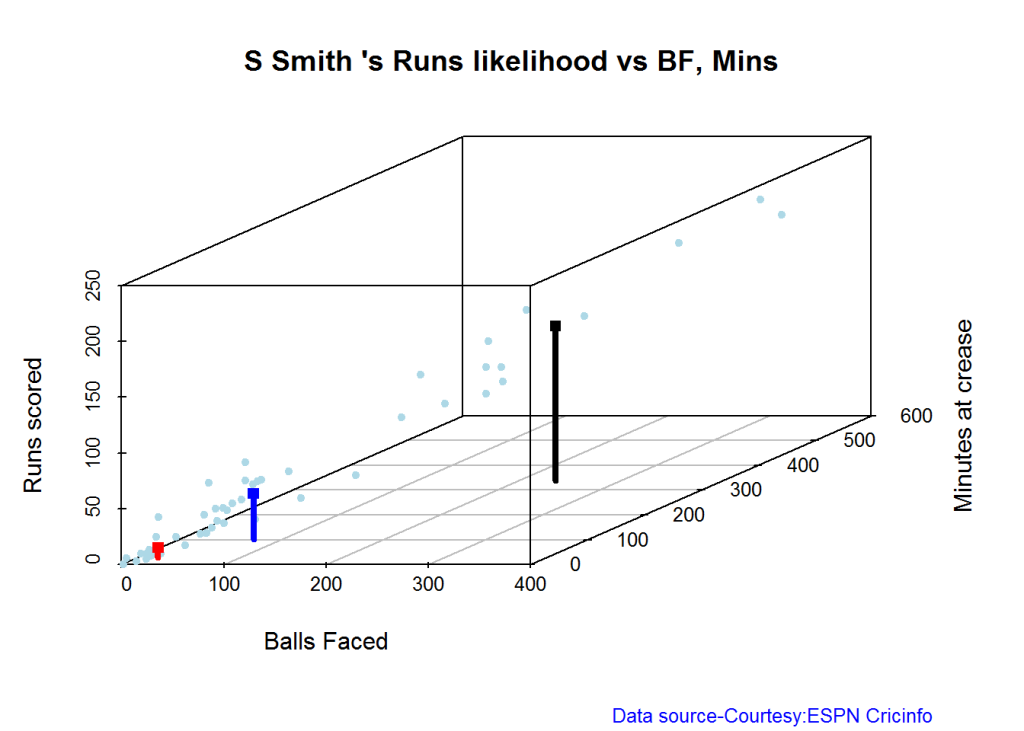
Highest runs likelihood
The plots below the runs likelihood of batsman. This uses K-Means. It can be seen Smith has the best likelihood around 40% of scoring around 41 runs, followed by Root who has 28.3% likelihood of scoring around 81 runs
A. Steven Smith
batsmanRunsLikelihood("./smith.csv","S Smith")

## Summary of S Smith 's runs scoring likelihood
## **************************************************
##
## There is a 40 % likelihood that S Smith will make 41 Runs in 73 balls over 101 Minutes
## There is a 36 % likelihood that S Smith will make 9 Runs in 21 balls over 27 Minutes
## There is a 24 % likelihood that S Smith will make 139 Runs in 237 balls over 338 MinutesB. David Warner
batsmanRunsLikelihood("./warner.csv","D Warner")


## Summary of D Warner 's runs scoring likelihood
## **************************************************
##
## There is a 11.11 % likelihood that D Warner will make 134 Runs in 159 balls over 263 Minutes
## There is a 63.89 % likelihood that D Warner will make 17 Runs in 25 balls over 37 Minutes
## There is a 25 % likelihood that D Warner will make 73 Runs in 105 balls over 156 MinutesC. Alastair Cook
batsmanRunsLikelihood("./cook.csv","A Cook")


## Summary of A Cook 's runs scoring likelihood
## **************************************************
##
## There is a 27.72 % likelihood that A Cook will make 64 Runs in 140 balls over 195 Minutes
## There is a 59.9 % likelihood that A Cook will make 15 Runs in 32 balls over 46 Minutes
## There is a 12.38 % likelihood that A Cook will make 141 Runs in 300 balls over 420 MinutesD. J E Root
batsmanRunsLikelihood("./root.csv","JE Root")


## Summary of JE Root 's runs scoring likelihood
## **************************************************
##
## There is a 28.3 % likelihood that JE Root will make 81 Runs in 158 balls over 223 Minutes
## There is a 7.55 % likelihood that JE Root will make 179 Runs in 290 balls over 425 Minutes
## There is a 64.15 % likelihood that JE Root will make 16 Runs in 39 balls over 59 Minutes Average runs at ground and against opposition
A. Steven Smith
par(mfrow=c(1,2))
par(mar=c(4,4,2,2))
batsmanAvgRunsGround("./smith.csv","S Smith")
batsmanAvgRunsOpposition("./smith.csv","S Smith")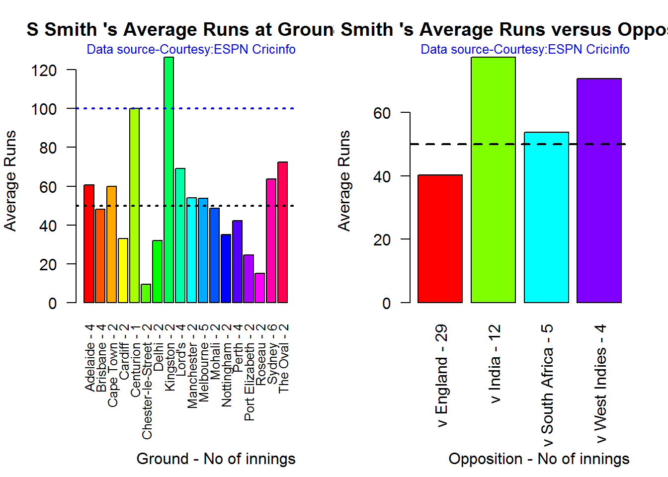
dev.off()## null device
## 1B. David Warner
par(mfrow=c(1,2))
par(mar=c(4,4,2,2))
batsmanAvgRunsGround("./warner.csv","D Warner")
batsmanAvgRunsOpposition("./warner.csv","D Warner")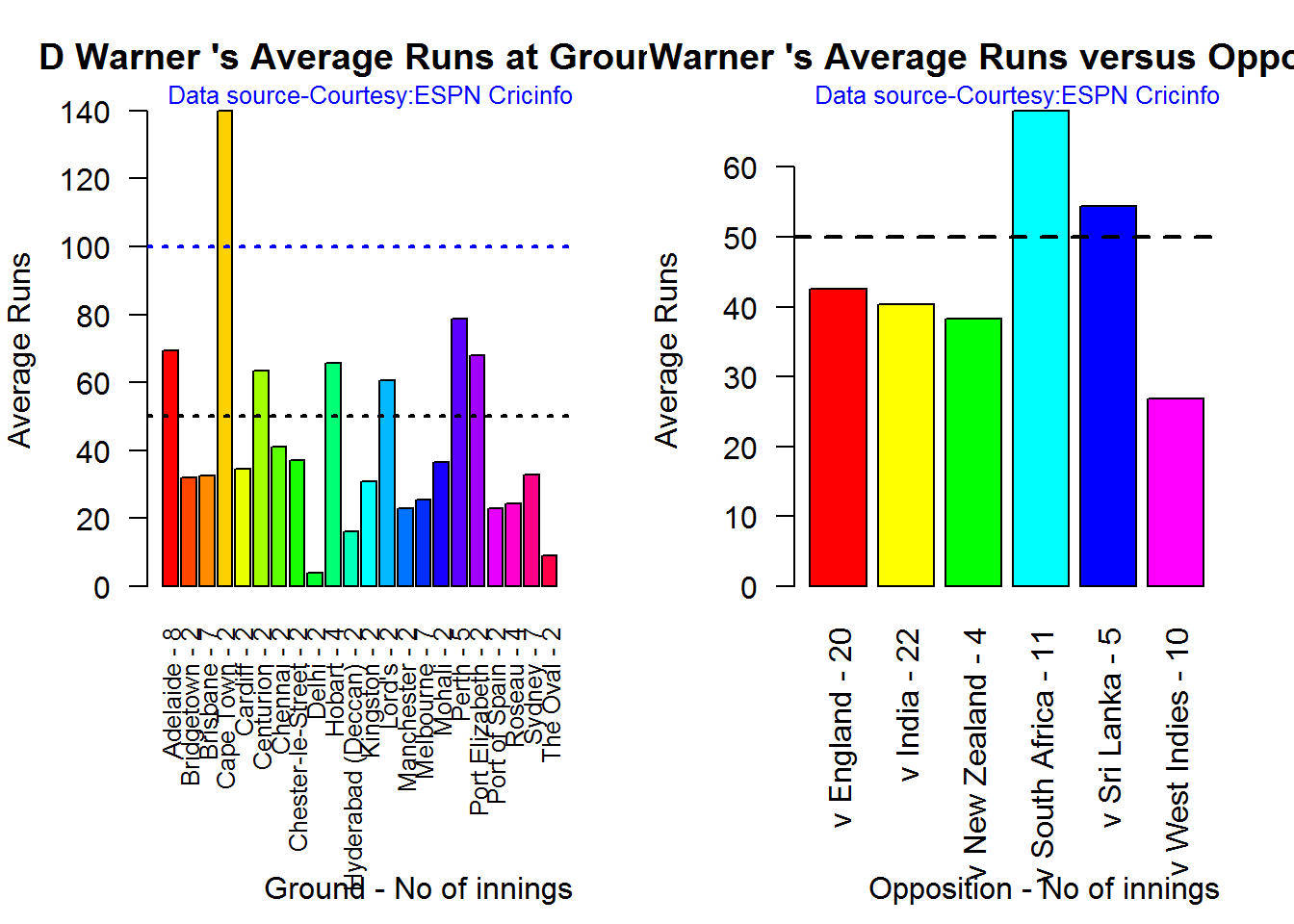
dev.off()## null device
## 1C. Alistair Cook
par(mfrow=c(1,2))
par(mar=c(4,4,2,2))
batsmanAvgRunsGround("./cook.csv","A Cook")
batsmanAvgRunsOpposition("./cook.csv","A Cook")
dev.off()## null device
## 1D. J E Root
par(mfrow=c(1,2))
par(mar=c(4,4,2,2))
batsmanAvgRunsGround("./root.csv","JE Root")
batsmanAvgRunsOpposition("./root.csv","JE Root")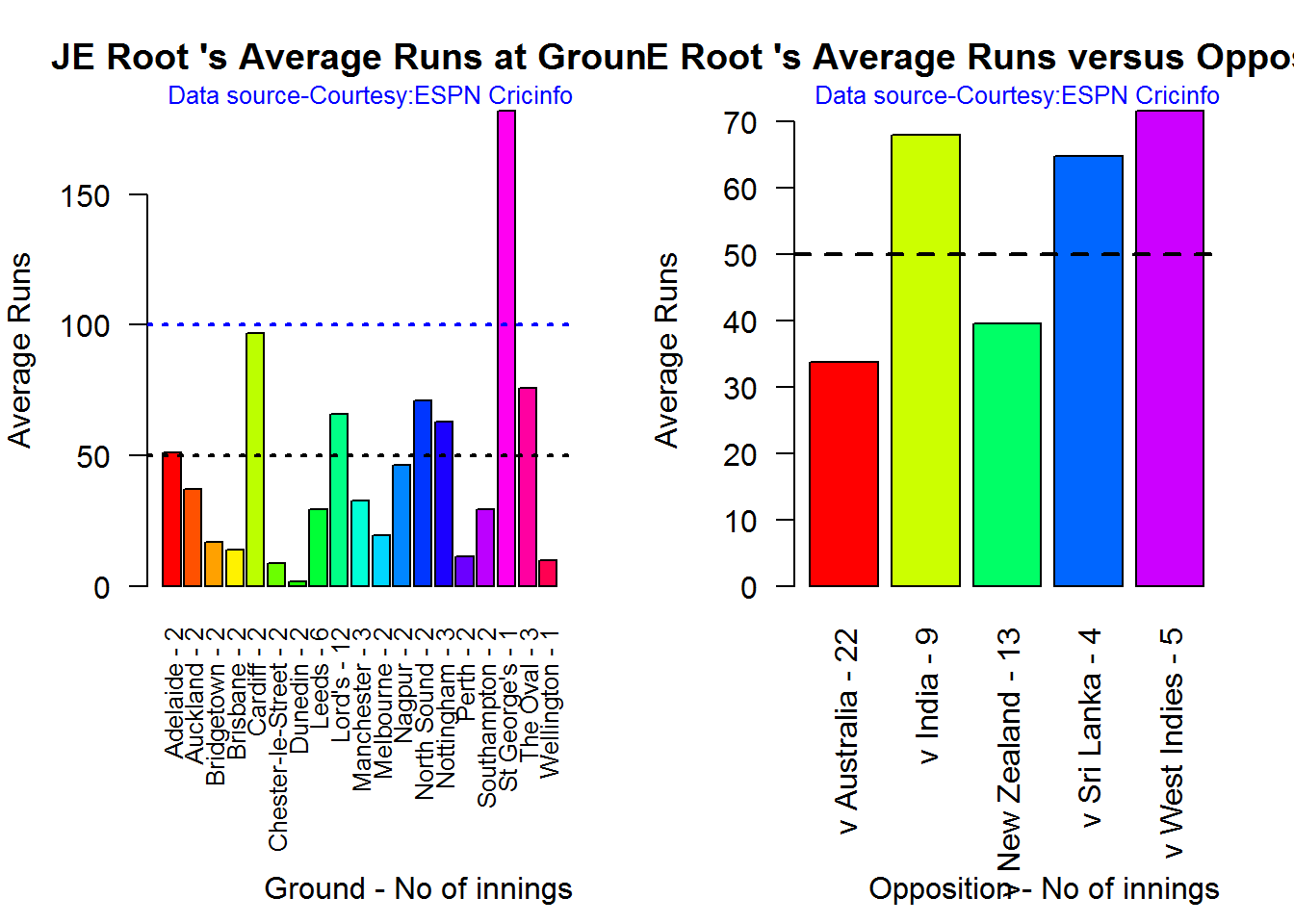
dev.off()## null device
## 1Analysis of bowlers
- Mitchell Johnson (Aus) – Innings-131, Wickets – 299, Econ Rate : 3.28
- Peter Siddle (Aus) – Innings – 104 , Wickets- 192, Econ Rate : 2.95
- James Anderson (Eng) – Innings – 199 , Wickets- 406, Econ Rate : 3.05
- Stuart Broad (Eng) – Innings – 148 , Wickets- 296, Econ Rate : 3.08
Anderson has the highest number of inning and wickets followed closely by Broad and Mitchell who are in a neck to neck race with respect to wickets. Johnson is on the more expensive side though. Siddle has fewer innings but a good economy rate.
Wicket Frequency percentage
This plot gives the percentage of wickets for each wickets (1,2,3…etc)
par(mfrow=c(1,4))
par(mar=c(4,4,2,2))
bowlerWktsFreqPercent("./johnson.csv","Johnson")
bowlerWktsFreqPercent("./siddle.csv","Siddle")
bowlerWktsFreqPercent("./broad.csv","Broad")
bowlerWktsFreqPercent("./anderson.csv","Anderson")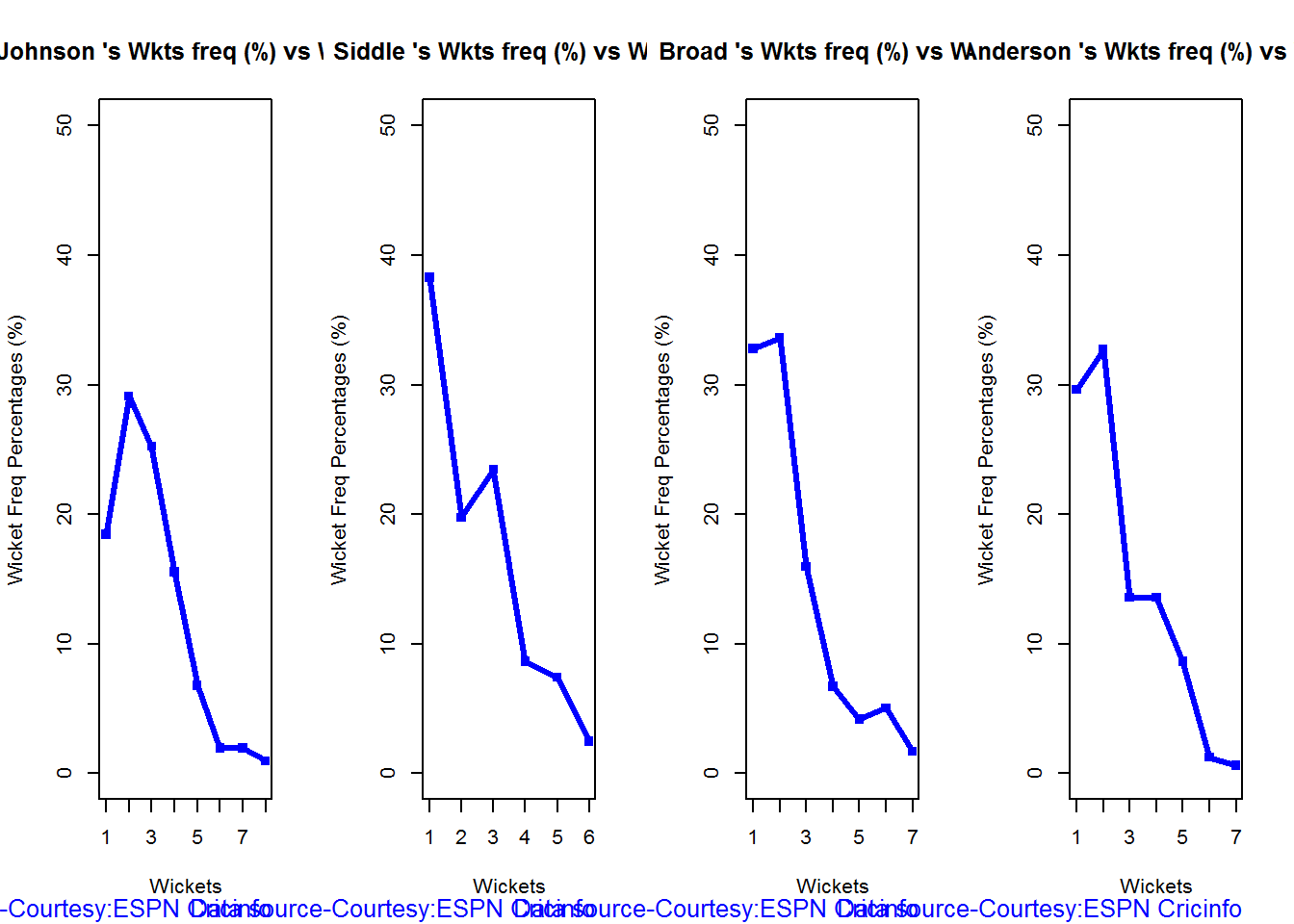
dev.off()## null device
## 1Wickets Runs plot
The plot below gives a boxplot of the runs ranges for each of the wickets taken by the bowlers
par(mfrow=c(1,4))
par(mar=c(4,4,2,2))
bowlerWktsRunsPlot("./johnson.csv","Johnson")
bowlerWktsRunsPlot("./siddle.csv","Siddle")
bowlerWktsRunsPlot("./broad.csv","Broad")
bowlerWktsRunsPlot("./anderson.csv","Anderson")
dev.off()## null device
## 1Average wickets in different grounds and opposition
A. Mitchell Johnson
par(mfrow=c(1,2))
par(mar=c(4,4,2,2))
bowlerAvgWktsGround("./johnson.csv","Johnson")
bowlerAvgWktsOpposition("./johnson.csv","Johnson")
dev.off()## null device
## 1B. Peter Siddle
par(mfrow=c(1,2))
par(mar=c(4,4,2,2))
bowlerAvgWktsGround("./siddle.csv","Siddle")
bowlerAvgWktsOpposition("./siddle.csv","Siddle")
dev.off()## null device
## 1C. Stuart Broad
par(mfrow=c(1,2))
par(mar=c(4,4,2,2))
bowlerAvgWktsGround("./broad.csv","Broad")
bowlerAvgWktsOpposition("./broad.csv","Broad")
dev.off()## null device
## 1D. James Anderson
par(mfrow=c(1,2))
par(mar=c(4,4,2,2))
bowlerAvgWktsGround("./anderson.csv","Anderson")
bowlerAvgWktsOpposition("./anderson.csv","Anderson")
dev.off()## null device
## 1Relative bowling performance
The plot below shows that Mitchell Johnson is the mopst effective bowler among the lot with a higher wickets in the 3-6 wicket range. Broad and Anderson seem to perform well in 2 wickets in comparison to Siddle but in 3 wickets Siddle is better than Broad and Anderson.
frames <- list("./johnson.csv","./siddle.csv","broad.csv","anderson.csv")
names <- list("Johnson","Siddle","Broad","Anderson")
relativeBowlingPerf(frames,names)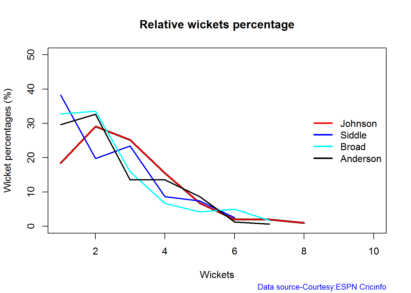
Relative Economy Rate against wickets taken
Anderson followed by Siddle has the best economy rates. Johnson is fairly expensive in the 4-8 wicket range.
frames <- list("./johnson.csv","./siddle.csv","broad.csv","anderson.csv")
names <- list("Johnson","Siddle","Broad","Anderson")
relativeBowlingER(frames,names)
Moving average of wickets over career
Johnson is on his second peak while Siddle is on the decline with respect to bowling. Broad and Anderson show improving performance over the years.
par(mfrow=c(2,2))
par(mar=c(4,4,2,2))
bowlerMovingAverage("./johnson.csv","Johnson")
bowlerMovingAverage("./siddle.csv","Siddle")
bowlerMovingAverage("./broad.csv","Broad")
bowlerMovingAverage("./anderson.csv","Anderson")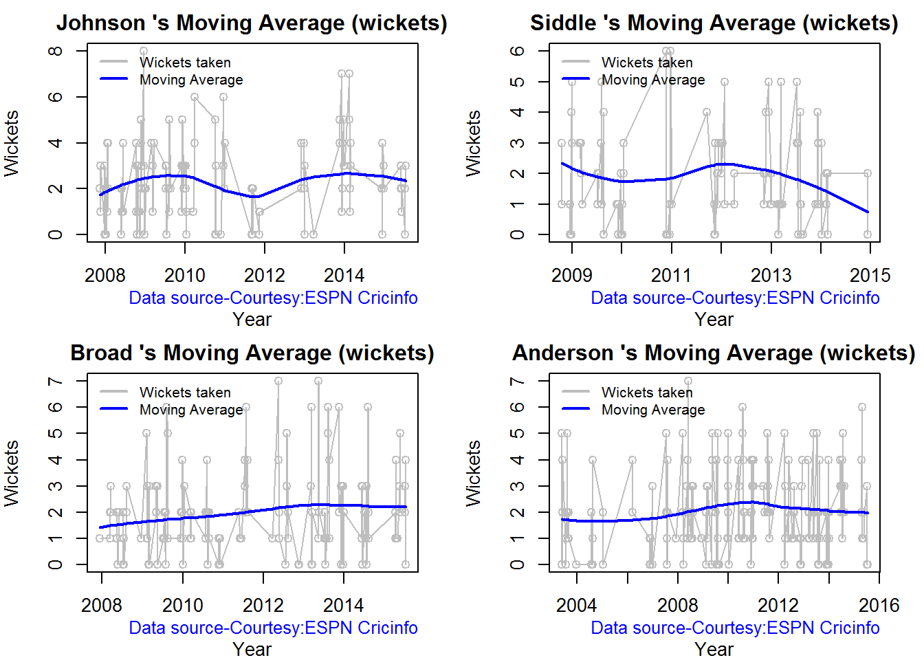
dev.off()## null device
## 1Wickets forecast
par(mfrow=c(2,2))
par(mar=c(4,4,2,2))
bowlerPerfForecast("./johnson.csv","Johnson")
bowlerPerfForecast("./siddle.csv","Siddle")
bowlerPerfForecast("./broad.csv","Broad")
bowlerPerfForecast("./anderson.csv","Anderson")
dev.off()## null device
## 1Key findings
Here are some key conclusions
- Cook has the most number of innings and has been extremly consistent in his scores
- Warner has the best strike rate among the lot followed by Smith and Root
- The moving average shows a marked improvement over the years for Smith
- Johnson is the most effective bowler but is fairly expensive
- Anderson has the best economy rate followed by Siddle
- Johnson is at his second peak with respect to bowling while Broad and Anderson maintain a steady line and length in their career bowling performance
Also see my other posts in R
- Introducing cricketr! : An R package to analyze performances of cricketers
- Taking cricketr for a spin – Part 1
- A peek into literacy in India: Statistical Learning with R
- A crime map of India in R – Crimes against women
- Analyzing cricket’s batting legends – Through the mirage with R
- Masters of Spin: Unraveling the web with R
- Mirror, mirror . the best batsman of them all?
You may also like
- A crime map of India in R: Crimes against women
- What’s up Watson? Using IBM Watson’s QAAPI with Bluemix, NodeExpress – Part 1
- Bend it like Bluemix, MongoDB with autoscaling – Part 2
- Informed choices through Machine Learning : Analyzing Kohli, Tendulkar and Dravid
- Thinking Web Scale (TWS-3): Map-Reduce – Bring compute to data
- Deblurring with OpenCV:Weiner filter reloaded
Share:

Introducing cricketr! : An R package to analyze performances of cricketers
Yet all experience is an arch wherethro’
Gleams that untravell’d world whose margin fades
For ever and forever when I move.
How dull it is to pause, to make an end,
To rust unburnish’d, not to shine in use!
Ulysses by Alfred Tennyson
Introduction
This is an initial post in which I introduce a cricketing package ‘cricketr’ which I have created. This package was a natural culmination to my earlier posts on cricket and my finishing 10 modules of Data Science Specialization, from John Hopkins University at Coursera. The thought of creating this package struck me some time back, and I have finally been able to bring this to fruition.
So here it is. My R package ‘cricketr!!!’
If you are passionate about cricket, and love analyzing cricket performances, then check out my racy book on cricket ‘Cricket analytics with cricketr and cricpy – Analytics harmony with R & Python’! This book discusses and shows how to use my R package ‘cricketr’ and my Python package ‘cricpy’ to analyze batsmen and bowlers in all formats of the game (Test, ODI and T20). The paperback is available on Amazon at $21.99 and the kindle version at $9.99/Rs 449/-. A must read for any cricket lover! Check it out!!
You can download the latest PDF version of the book at ‘Cricket analytics with cricketr and cricpy: Analytics harmony with R and Python-6th edition‘
This package uses the statistics info available in ESPN Cricinfo Statsguru. The current version of this package can handle all formats of the game including Test, ODI and Twenty20 cricket.
You should be able to install the package from CRAN and use many of the functions available in the package. Please be mindful of ESPN Cricinfo Terms of Use
(Note: This page is also hosted as a GitHub page at cricketr and also at RPubs as cricketr: A R package for analyzing performances of cricketers
You can download this analysis as a PDF file from Introducing cricketr
Note: If you would like to do a similar analysis for a different set of batsman and bowlers, you can clone/download my skeleton cricketr template from Github (which is the R Markdown file I have used for the analysis below). You will only need to make appropriate changes for the players you are interested in. Just a familiarity with R and R Markdown only is needed.
You can clone the cricketr code from Github at cricketr
(Take a look at my short video tutorial on my R package cricketr on Youtube – R package cricketr – A short tutorial)
Do check out my interactive Shiny app implementation using the cricketr package – Sixer – R package cricketr’s new Shiny avatar
Please look at my recent post, which includes updates to this post, and 8 new functions added to the cricketr package “Re-introducing cricketr: An R package to analyze the performances of cricketers”
Important note 1: The latest release of ‘cricketr’ now includes the ability to analyze performances of teams now!! See Cricketr adds team analytics to its repertoire!!!
Important note 2 : Cricketr can now do a more fine-grained analysis of players, see Cricketr learns new tricks : Performs fine-grained analysis of players
Important note 3: Do check out the python avatar of cricketr, ‘cricpy’ in my post ‘Introducing cricpy:A python package to analyze performances of cricketers”
The cricketr package
The cricketr package has several functions that perform several different analyses on both batsman and bowlers. The package has functions that plot percentage frequency runs or wickets, runs likelihood for a batsman, relative run/strike rates of batsman and relative performance/economy rate for bowlers are available.
Other interesting functions include batting performance moving average, forecast and a function to check whether the batsman/bowler is in in-form or out-of-form.
The data for a particular player can be obtained with the getPlayerData() function from the package. To do this you will need to go to ESPN CricInfo Player and type in the name of the player for e.g Ricky Ponting, Sachin Tendulkar etc. This will bring up a page which have the profile number for the player e.g. for Sachin Tendulkar this would be http://www.espncricinfo.com/india/content/player/35320.html. Hence, Sachin’s profile is 35320. This can be used to get the data for Tendulkar as shown below
The cricketr package is now available from CRAN!!!. You should be able to install directly with
if (!require("cricketr")){
install.packages("cricketr",lib = "c:/test")
}
library(cricketr)
?getPlayerData##
## getPlayerData(profile, opposition='', host='', dir='./data', file='player001.csv', type='batting', homeOrAway=[1, 2], result=[1, 2, 4], create=True)
## Get the player data from ESPN Cricinfo based on specific inputs and store in a file in a given directory
##
## Description
##
## Get the player data given the profile of the batsman. The allowed inputs are home,away or both and won,lost or draw of matches. The data is stored in a .csv file in a directory specified. This function also returns a data frame of the player
##
## Usage
##
## getPlayerData(profile,opposition="",host="",dir="./data",file="player001.csv",
## type="batting", homeOrAway=c(1,2),result=c(1,2,4))
## Arguments
##
## profile
## This is the profile number of the player to get data. This can be obtained from http://www.espncricinfo.com/ci/content/player/index.html. Type the name of the player and click search. This will display the details of the player. Make a note of the profile ID. For e.g For Sachin Tendulkar this turns out to be http://www.espncricinfo.com/india/content/player/35320.html. Hence the profile for Sachin is 35320
## opposition
## The numerical value of the opposition country e.g.Australia,India, England etc. The values are Australia:2,Bangladesh:25,England:1,India:6,New Zealand:5,Pakistan:7,South Africa:3,Sri Lanka:8, West Indies:4, Zimbabwe:9
## host
## The numerical value of the host country e.g.Australia,India, England etc. The values are Australia:2,Bangladesh:25,England:1,India:6,New Zealand:5,Pakistan:7,South Africa:3,Sri Lanka:8, West Indies:4, Zimbabwe:9
## dir
## Name of the directory to store the player data into. If not specified the data is stored in a default directory "./data". Default="./data"
## file
## Name of the file to store the data into for e.g. tendulkar.csv. This can be used for subsequent functions. Default="player001.csv"
## type
## type of data required. This can be "batting" or "bowling"
## homeOrAway
## This is a vector with either 1,2 or both. 1 is for home 2 is for away
## result
## This is a vector that can take values 1,2,4. 1 - won match 2- lost match 4- draw
## Details
##
## More details can be found in my short video tutorial in Youtube https://www.youtube.com/watch?v=q9uMPFVsXsI
##
## Value
##
## Returns the player's dataframe
##
## Note
##
## Maintainer: Tinniam V Ganesh <tvganesh.85@gmail.com>
##
## Author(s)
##
## Tinniam V Ganesh
##
## References
##
## http://www.espncricinfo.com/ci/content/stats/index.html
## https://gigadom.wordpress.com/
##
## See Also
##
## getPlayerDataSp
##
## Examples
##
## ## Not run:
## # Both home and away. Result = won,lost and drawn
## tendulkar = getPlayerData(35320,dir=".", file="tendulkar1.csv",
## type="batting", homeOrAway=c(1,2),result=c(1,2,4))
##
## # Only away. Get data only for won and lost innings
## tendulkar = getPlayerData(35320,dir=".", file="tendulkar2.csv",
## type="batting",homeOrAway=c(2),result=c(1,2))
##
## # Get bowling data and store in file for future
## kumble = getPlayerData(30176,dir=".",file="kumble1.csv",
## type="bowling",homeOrAway=c(1),result=c(1,2))
##
## #Get the Tendulkar's Performance against Australia in Australia
## tendulkar = getPlayerData(35320, opposition = 2,host=2,dir=".",
## file="tendulkarVsAusInAus.csv",type="batting")The cricketr package includes some pre-packaged sample (.csv) files. You can use these sample to test functions as shown below
# Retrieve the file path of a data file installed with cricketr
pathToFile ,"Sachin Tendulkar")

Alternatively, the cricketr package can be installed from GitHub with
if (!require("cricketr")){
library(devtools)
install_github("tvganesh/cricketr")
}
library(cricketr)
The pre-packaged files can be accessed as shown above.
To get the data of any player use the function getPlayerData()
tendulkar <- getPlayerData(35320,dir="..",file="tendulkar.csv",type="batting",homeOrAway=c(1,2),
result=c(1,2,4))Important Note This needs to be done only once for a player. This function stores the player’s data in a CSV file (for e.g. tendulkar.csv as above) which can then be reused for all other functions. Once we have the data for the players many analyses can be done. This post will use the stored CSV file obtained with a prior getPlayerData for all subsequent analyses
Sachin Tendulkar’s performance – Basic Analyses
The 3 plots below provide the following for Tendulkar
- Frequency percentage of runs in each run range over the whole career
- Mean Strike Rate for runs scored in the given range
- A histogram of runs frequency percentages in runs ranges
par(mfrow=c(1,3))
par(mar=c(4,4,2,2))
batsmanRunsFreqPerf("./tendulkar.csv","Sachin Tendulkar")
batsmanMeanStrikeRate("./tendulkar.csv","Sachin Tendulkar")
batsmanRunsRanges("./tendulkar.csv","Sachin Tendulkar")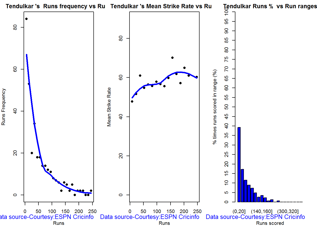
dev.off()## null device
## 1
More analyses
par(mfrow=c(1,3))
par(mar=c(4,4,2,2))
batsman4s("./tendulkar.csv","Tendulkar")
batsman6s("./tendulkar.csv","Tendulkar")
batsmanDismissals("./tendulkar.csv","Tendulkar")
3D scatter plot and prediction plane
The plots below show the 3D scatter plot of Sachin’s Runs versus Balls Faced and Minutes at crease. A linear regression model is then fitted between Runs and Balls Faced + Minutes at crease
battingPerf3d("./tendulkar.csv","Sachin Tendulkar")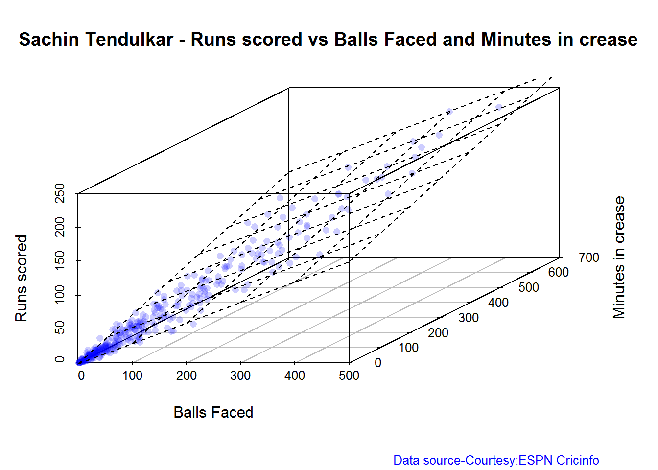
Average runs at different venues
The plot below gives the average runs scored by Tendulkar at different grounds. The plot also displays the number of innings at each ground as a label at x-axis. It can be seen Tendulkar did great in Colombo (SSC), Melbourne ifor matches overseas and Mumbai, Mohali and Bangalore at home
batsmanAvgRunsGround("./tendulkar.csv","Sachin Tendulkar")


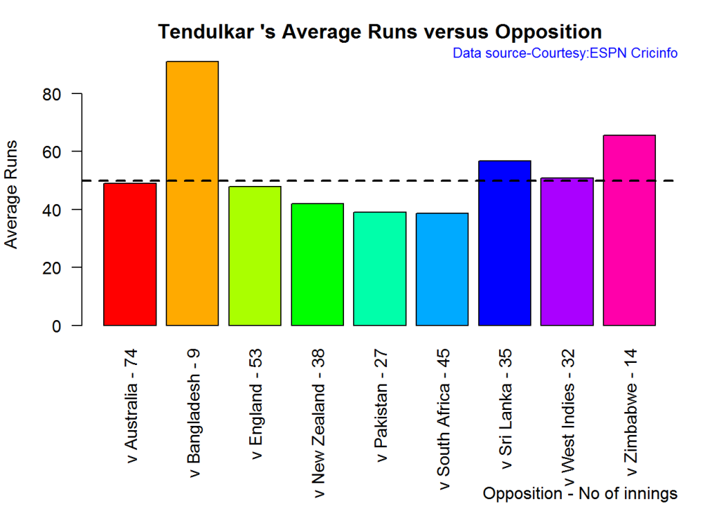
Average runs against different opposing teams
This plot computes the average runs scored by Tendulkar against different countries. The x-axis also gives the number of innings against each team
batsmanAvgRunsOpposition("./tendulkar.csv","Tendulkar")

Highest Runs Likelihood
The plot below shows the Runs Likelihood for a batsman. For this the performance of Sachin is plotted as a 3D scatter plot with Runs versus Balls Faced + Minutes at crease using. K-Means. The centroids of 3 clusters are computed and plotted. In this plot. Sachin Tendulkar’s highest tendencies are computed and plotted using K-Means
batsmanRunsLikelihood("./tendulkar.csv","Sachin Tendulkar")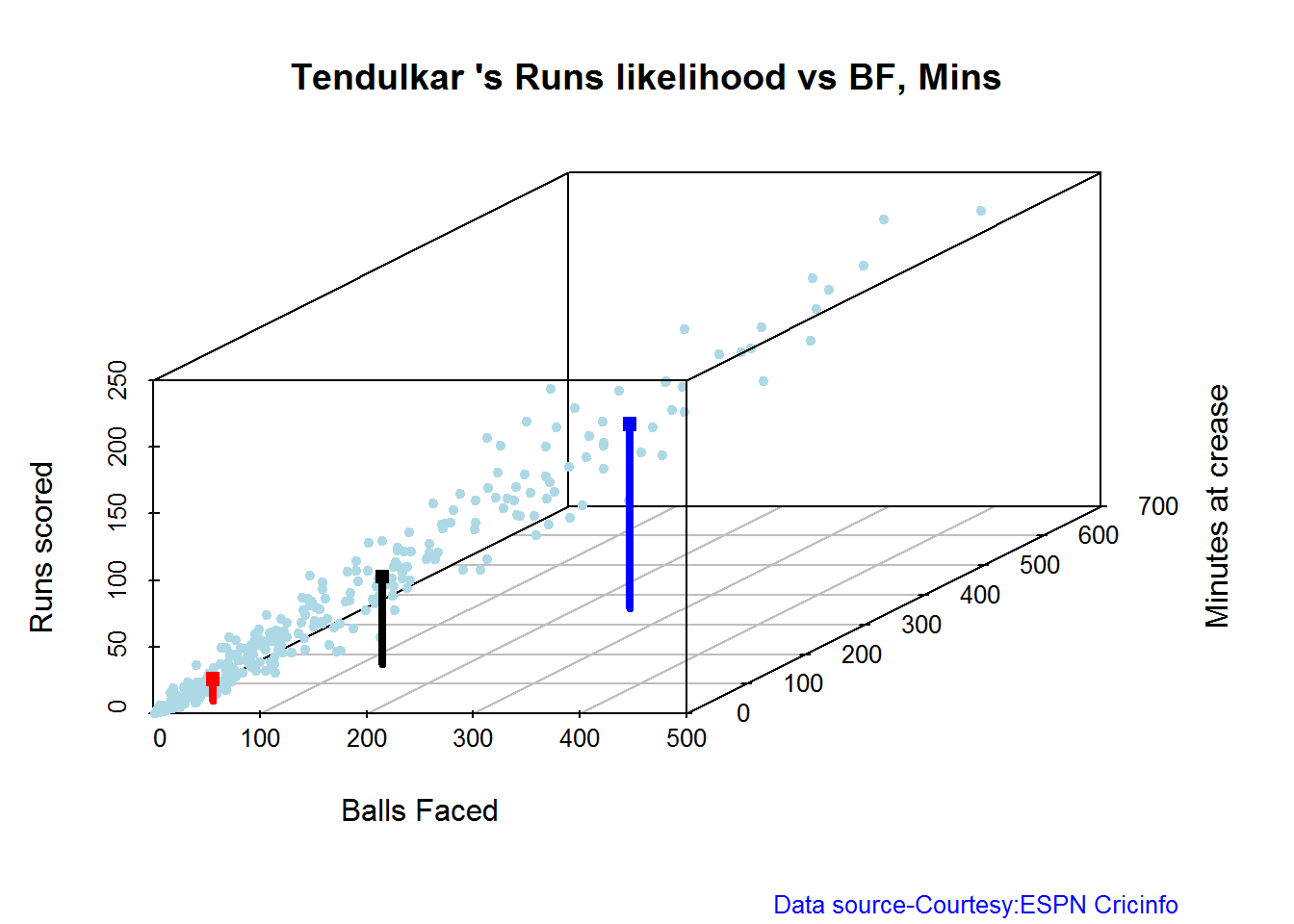
## Summary of Sachin Tendulkar 's runs scoring likelihood
## **************************************************
##
## There is a 16.51 % likelihood that Sachin Tendulkar will make 139 Runs in 251 balls over 353 Minutes
## There is a 58.41 % likelihood that Sachin Tendulkar will make 16 Runs in 31 balls over 44 Minutes
## There is a 25.08 % likelihood that Sachin Tendulkar will make 66 Runs in 122 balls over 167 MinutesA look at the Top 4 batsman – Tendulkar, Kallis, Ponting and Sangakkara
The batsmen with the most hundreds in test cricket are
- Sachin Tendulkar :Average:53.78,100’s – 51, 50’s – 68
- Jacques Kallis : Average: 55.47, 100’s – 45, 50’s – 58
- Ricky Ponting : Average: 51.85, 100’s – 41 , 50’s – 62
- Kumara Sangakarra: Average: 58.04 ,100’s – 38 , 50’s – 52
in that order.
The following plots take a closer at their performances. The box plots show the mean (red line) and median (blue line). The two ends of the boxplot display the 25th and 75th percentile.
Box Histogram Plot
This plot shows a combined boxplot of the Runs ranges and a histogram of the Runs Frequency. The calculated Mean differ from the stated means possibly because of data cleaning. Also not sure how the means were arrived at ESPN Cricinfo for e.g. when considering not out..
batsmanPerfBoxHist("./tendulkar.csv","Sachin Tendulkar")
batsmanPerfBoxHist("./kallis.csv","Jacques Kallis")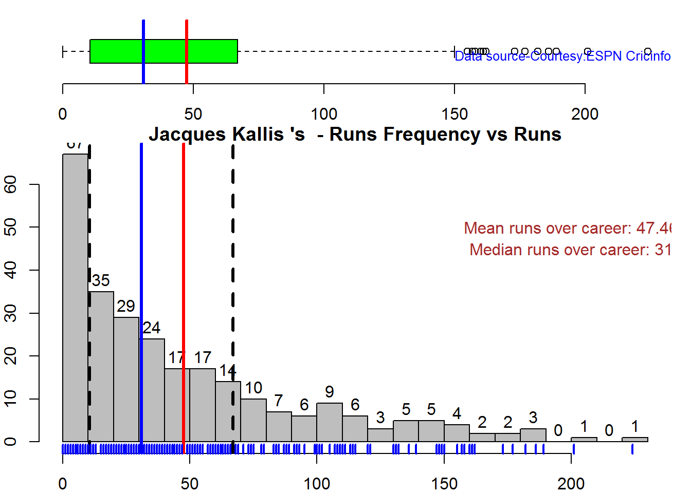
batsmanPerfBoxHist("./ponting.csv","Ricky Ponting")
batsmanPerfBoxHist("./sangakkara.csv","K Sangakkara")
Contribution to won and lost matches
The plot below shows the contribution of Tendulkar, Kallis, Ponting and Sangakarra in matches won and lost. The plots show the range of runs scored as a boxplot (25th & 75th percentile) and the mean scored. The total matches won and lost are also printed in the plot.
All the players have scored more in the matches they won than the matches they lost. Ricky Ponting is the only batsman who seems to have more matches won to his credit than others. This could also be because he was a member of strong Australian team
For the next 2 functions below you will have to use the getPlayerDataSp() function. I
have commented this as I already have these files
tendulkarsp par(mfrow=c(2,2))
par(mar=c(4,4,2,2))
batsmanContributionWonLost("tendulkarsp.csv","Tendulkar")
batsmanContributionWonLost("kallissp.csv","Kallis")
batsmanContributionWonLost("pontingsp.csv","Ponting")
batsmanContributionWonLost("sangakkarasp.csv","Sangakarra")
dev.off()## null device
## 1
Performance at home and overseas
From the plot below it can be seen
Tendulkar has more matches overseas than at home and his performance is consistent in all venues at home or abroad. Ponting has lesser innings than Tendulkar and has an equally good performance at home and overseas.Kallis and Sangakkara’s performance abroad is lower than the performance at home.
This function also requires the use of getPlayerDataSp() as shown above
par(mfrow=c(2,2))
par(mar=c(4,4,2,2))
batsmanPerfHomeAway("tendulkarsp.csv","Tendulkar")
batsmanPerfHomeAway("kallissp.csv","Kallis")
batsmanPerfHomeAway("pontingsp.csv","Ponting")
batsmanPerfHomeAway("sangakkarasp.csv","Sangakarra")
dev.off()


dev.off()## null device
## 1 Relative Mean Strike Rate plot
The plot below compares the Mean Strike Rate of the batsman for each of the runs ranges of 10 and plots them. The plot indicate the following Range 0 – 50 Runs – Ponting leads followed by Tendulkar Range 50 -100 Runs – Ponting followed by Sangakkara Range 100 – 150 – Ponting and then Tendulkar
frames <- list("./tendulkar.csv","./kallis.csv","ponting.csv","sangakkara.csv")
names <- list("Tendulkar","Kallis","Ponting","Sangakkara")
relativeBatsmanSR(frames,names)
Relative Runs Frequency plot
The plot below gives the relative Runs Frequency Percetages for each 10 run bucket. The plot below show
Sangakkara leads followed by Ponting
frames <- list("./tendulkar.csv","./kallis.csv","ponting.csv","sangakkara.csv")
names <- list("Tendulkar","Kallis","Ponting","Sangakkara")
relativeRunsFreqPerf(frames,names)
Moving Average of runs in career
Take a look at the Moving Average across the career of the Top 4. Clearly . Kallis and Sangakkara have a few more years of great batting ahead. They seem to average on 50. . Tendulkar and Ponting definitely show a slump in the later years
par(mfrow=c(2,2))
par(mar=c(4,4,2,2))
batsmanMovingAverage("./tendulkar.csv","Sachin Tendulkar")
batsmanMovingAverage("./kallis.csv","Jacques Kallis")
batsmanMovingAverage("./ponting.csv","Ricky Ponting")
batsmanMovingAverage("./sangakkara.csv","K Sangakkara")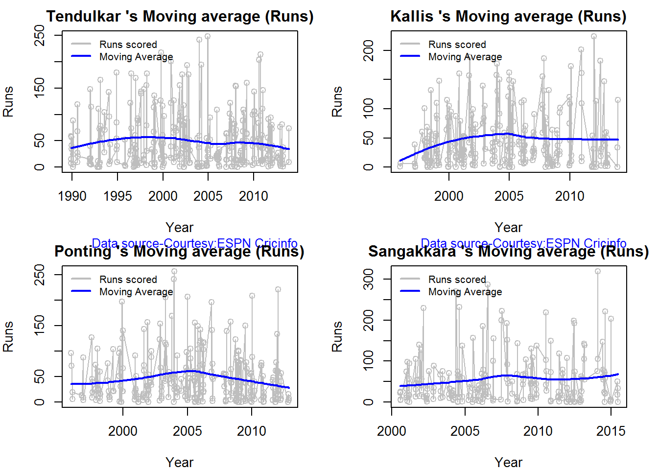
dev.off()## null device
## 1Future Runs forecast
Here are plots that forecast how the batsman will perform in future. In this case 90% of the career runs trend is uses as the training set. the remaining 10% is the test set.
A Holt-Winters forecating model is used to forecast future performance based on the 90% training set. The forecated runs trend is plotted. The test set is also plotted to see how close the forecast and the actual matches
Take a look at the runs forecasted for the batsman below.
- Tendulkar’s forecasted performance seems to tally with his actual performance with an average of 50
- Kallis the forecasted runs are higher than the actual runs he scored
- Ponting seems to have a good run in the future
- Sangakkara has a decent run in the future averaging 50 runs
par(mfrow=c(2,2))
par(mar=c(4,4,2,2))
batsmanPerfForecast("./tendulkar.csv","Sachin Tendulkar")
batsmanPerfForecast("./kallis.csv","Jacques Kallis")
batsmanPerfForecast("./ponting.csv","Ricky Ponting")
batsmanPerfForecast("./sangakkara.csv","K Sangakkara")
dev.off()## null device
## 1Check Batsman In-Form or Out-of-Form
The below computation uses Null Hypothesis testing and p-value to determine if the batsman is in-form or out-of-form. For this 90% of the career runs is chosen as the population and the mean computed. The last 10% is chosen to be the sample set and the sample Mean and the sample Standard Deviation are caculated.
The Null Hypothesis (H0) assumes that the batsman continues to stay in-form where the sample mean is within 95% confidence interval of population mean The Alternative (Ha) assumes that the batsman is out of form the sample mean is beyond the 95% confidence interval of the population mean.
A significance value of 0.05 is chosen and p-value us computed If p-value >= .05 – Batsman In-Form If p-value < 0.05 – Batsman Out-of-Form
Note Ideally the p-value should be done for a population that follows the Normal Distribution. But the runs population is usually left skewed. So some correction may be needed. I will revisit this later
This is done for the Top 4 batsman
checkBatsmanInForm("./tendulkar.csv","Sachin Tendulkar")## *******************************************************************************************
##
## Population size: 294 Mean of population: 50.48
## Sample size: 33 Mean of sample: 32.42 SD of sample: 29.8
##
## Null hypothesis H0 : Sachin Tendulkar 's sample average is within 95% confidence interval
## of population average
## Alternative hypothesis Ha : Sachin Tendulkar 's sample average is below the 95% confidence
## interval of population average
##
## [1] "Sachin Tendulkar 's Form Status: Out-of-Form because the p value: 0.000713 is less than alpha= 0.05"
## *******************************************************************************************checkBatsmanInForm("./kallis.csv","Jacques Kallis")## *******************************************************************************************
##
## Population size: 240 Mean of population: 47.5
## Sample size: 27 Mean of sample: 47.11 SD of sample: 59.19
##
## Null hypothesis H0 : Jacques Kallis 's sample average is within 95% confidence interval
## of population average
## Alternative hypothesis Ha : Jacques Kallis 's sample average is below the 95% confidence
## interval of population average
##
## [1] "Jacques Kallis 's Form Status: In-Form because the p value: 0.48647 is greater than alpha= 0.05"
## *******************************************************************************************checkBatsmanInForm("./ponting.csv","Ricky Ponting")## *******************************************************************************************
##
## Population size: 251 Mean of population: 47.5
## Sample size: 28 Mean of sample: 36.25 SD of sample: 48.11
##
## Null hypothesis H0 : Ricky Ponting 's sample average is within 95% confidence interval
## of population average
## Alternative hypothesis Ha : Ricky Ponting 's sample average is below the 95% confidence
## interval of population average
##
## [1] "Ricky Ponting 's Form Status: In-Form because the p value: 0.113115 is greater than alpha= 0.05"
## *******************************************************************************************checkBatsmanInForm("./sangakkara.csv","K Sangakkara")## *******************************************************************************************
##
## Population size: 193 Mean of population: 51.92
## Sample size: 22 Mean of sample: 71.73 SD of sample: 82.87
##
## Null hypothesis H0 : K Sangakkara 's sample average is within 95% confidence interval
## of population average
## Alternative hypothesis Ha : K Sangakkara 's sample average is below the 95% confidence
## interval of population average
##
## [1] "K Sangakkara 's Form Status: In-Form because the p value: 0.862862 is greater than alpha= 0.05"
## *******************************************************************************************3D plot of Runs vs Balls Faced and Minutes at Crease
The plot is a scatter plot of Runs vs Balls faced and Minutes at Crease. A prediction plane is fitted
par(mfrow=c(1,2))
par(mar=c(4,4,2,2))
battingPerf3d("./tendulkar.csv","Tendulkar")
battingPerf3d("./kallis.csv","Kallis")
 par(mfrow=c(1,2))
par(mar=c(4,4,2,2))
battingPerf3d("./ponting.csv","Ponting")
battingPerf3d("./sangakkara.csv","Sangakkara")
par(mfrow=c(1,2))
par(mar=c(4,4,2,2))
battingPerf3d("./ponting.csv","Ponting")
battingPerf3d("./sangakkara.csv","Sangakkara")
 dev.off()

## null device
## 1Predicting Runs given Balls Faced and Minutes at Crease
A multi-variate regression plane is fitted between Runs and Balls faced +Minutes at crease. A sample sequence of Balls Faced(BF) and Minutes at crease (Mins) is setup as shown below. The fitted model is used to predict the runs for these values
BF <- seq( 10, 400,length=15)
Mins <- seq(30,600,length=15)
newDF <- data.frame(BF,Mins)
tendulkar <- batsmanRunsPredict("./tendulkar.csv","Tendulkar",newdataframe=newDF)
kallis <- batsmanRunsPredict("./kallis.csv","Kallis",newdataframe=newDF)
ponting <- batsmanRunsPredict("./ponting.csv","Ponting",newdataframe=newDF)
sangakkara <- batsmanRunsPredict("./sangakkara.csv","Sangakkara",newdataframe=newDF)
The fitted model is then used to predict the runs that the batsmen will score for a given Balls faced and Minutes at crease. It can be seen Ponting has the will score the highest for a given Balls Faced and Minutes at crease.
Ponting is followed by Tendulkar who has Sangakkara close on his heels and finally we have Kallis. This is intuitive as we have already seen that Ponting has a highest strike rate.
batsmen <-cbind(round(tendulkar$Runs),round(kallis$Runs),round(ponting$Runs),round(sangakkara$Runs))
colnames(batsmen) <- c("Tendulkar","Kallis","Ponting","Sangakkara")
newDF <- data.frame(round(newDF$BF),round(newDF$Mins))
colnames(newDF) <- c("BallsFaced","MinsAtCrease")
predictedRuns <- cbind(newDF,batsmen)
predictedRuns
## BallsFaced MinsAtCrease Tendulkar Kallis Ponting Sangakkara
## 1 10 30 7 6 9 2
## 2 38 71 23 20 25 18
## 3 66 111 39 34 42 34
## 4 94 152 54 48 59 50
## 5 121 193 70 62 76 66
## 6 149 234 86 76 93 82
## 7 177 274 102 90 110 98
## 8 205 315 118 104 127 114
## 9 233 356 134 118 144 130
## 10 261 396 150 132 161 146
## 11 289 437 165 146 178 162
## 12 316 478 181 159 194 178
## 13 344 519 197 173 211 194
## 14 372 559 213 187 228 210
## 15 400 600 229 201 245 226 Checkout my book ‘Deep Learning from first principles Second Edition- In vectorized Python, R and Octave’. My book is available on Amazon as paperback ($18.99) and in kindle version($9.99/Rs449).
You may also like my companion book “Practical Machine Learning with R and Python:Second Edition- Machine Learning in stereo” available in Amazon in paperback($12.99) and Kindle($9.99/Rs449) versions.
Analysis of Top 3 wicket takers
The top 3 wicket takes in test history are
1. M Muralitharan:Wickets: 800, Average = 22.72, Economy Rate – 2.47
2. Shane Warne: Wickets: 708, Average = 25.41, Economy Rate – 2.65
3. Anil Kumble: Wickets: 619, Average = 29.65, Economy Rate – 2.69
How do Anil Kumble, Shane Warne and M Muralitharan compare with one another with respect to wickets taken and the Economy Rate. The next set of plots compute and plot precisely these analyses.
Wicket Frequency Plot
This plot below computes the percentage frequency of number of wickets taken for e.g 1 wicket x%, 2 wickets y% etc and plots them as a continuous line
par(mfrow=c(1,3))
par(mar=c(4,4,2,2))
bowlerWktsFreqPercent("./kumble.csv","Anil Kumble")
bowlerWktsFreqPercent("./warne.csv","Shane Warne")
bowlerWktsFreqPercent("./murali.csv","M Muralitharan")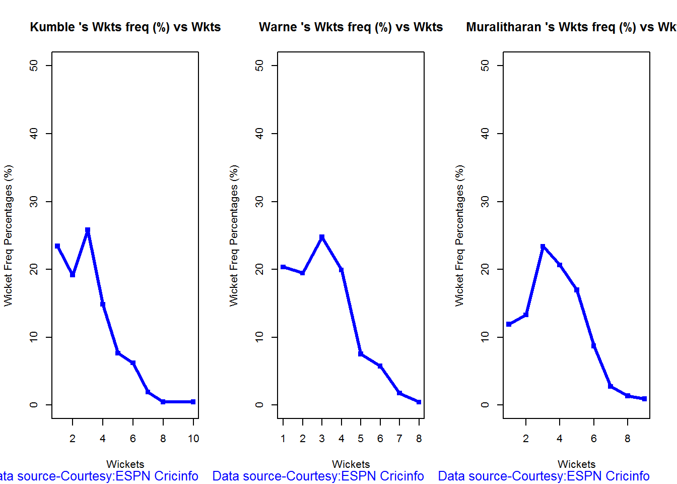
dev.off()## null device
## 1
Wickets Runs plot
par(mfrow=c(1,3))
par(mar=c(4,4,2,2))
bowlerWktsRunsPlot("./kumble.csv","Kumble")
bowlerWktsRunsPlot("./warne.csv","Warne")
bowlerWktsRunsPlot("./murali.csv","Muralitharan")


dev.off()## null device
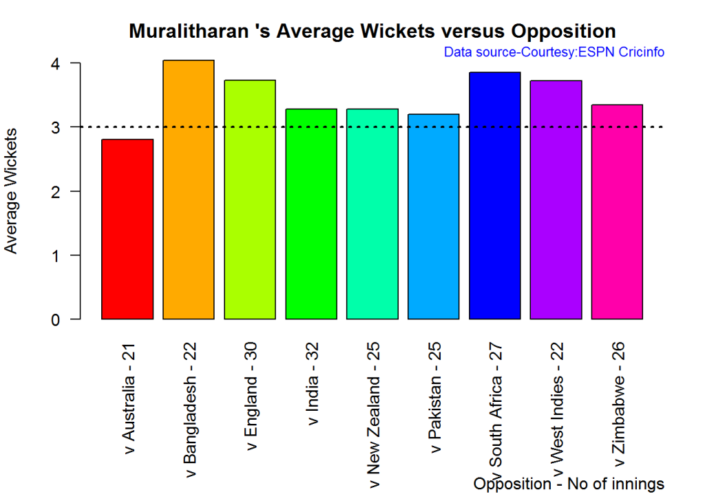
## 1Average wickets at different venues
The plot gives the average wickets taken by Muralitharan at different venues. Muralitharan has taken an average of 8 and 6 wickets at Oval & Wellington respectively in 2 different innings. His best performances are at Kandy and Colombo (SSC)
bowlerAvgWktsGround("./murali.csv","Muralitharan")

Average wickets against different opposition
The plot gives the average wickets taken by Muralitharan against different countries. The x-axis also includes the number of innings against each team
bowlerAvgWktsOpposition("./murali.csv","Muralitharan")

Relative Wickets Frequency Percentage
The Relative Wickets Percentage plot shows that M Muralitharan has a large percentage of wickets in the 3-8 wicket range
frames <- list("./kumble.csv","./murali.csv","warne.csv")
names <- list("Anil KUmble","M Muralitharan","Shane Warne")
relativeBowlingPerf(frames,names)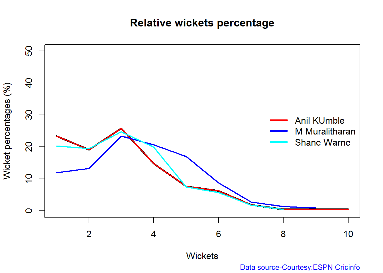
Relative Economy Rate against wickets taken
Clearly from the plot below it can be seen that Muralitharan has the best Economy Rate among the three
frames <- list("./kumble.csv","./murali.csv","warne.csv")
names <- list("Anil KUmble","M Muralitharan","Shane Warne")
relativeBowlingER(frames,names)
Wickets taken moving average
From th eplot below it can be see 1. Shane Warne’s performance at the time of his retirement was still at a peak of 3 wickets 2. M Muralitharan seems to have become ineffective over time with his peak years being 2004-2006 3. Anil Kumble also seems to slump down and become less effective.
par(mfrow=c(1,3))
par(mar=c(4,4,2,2))
bowlerMovingAverage("./kumble.csv","Anil Kumble")
bowlerMovingAverage("./warne.csv","Shane Warne")
bowlerMovingAverage("./murali.csv","M Muralitharan")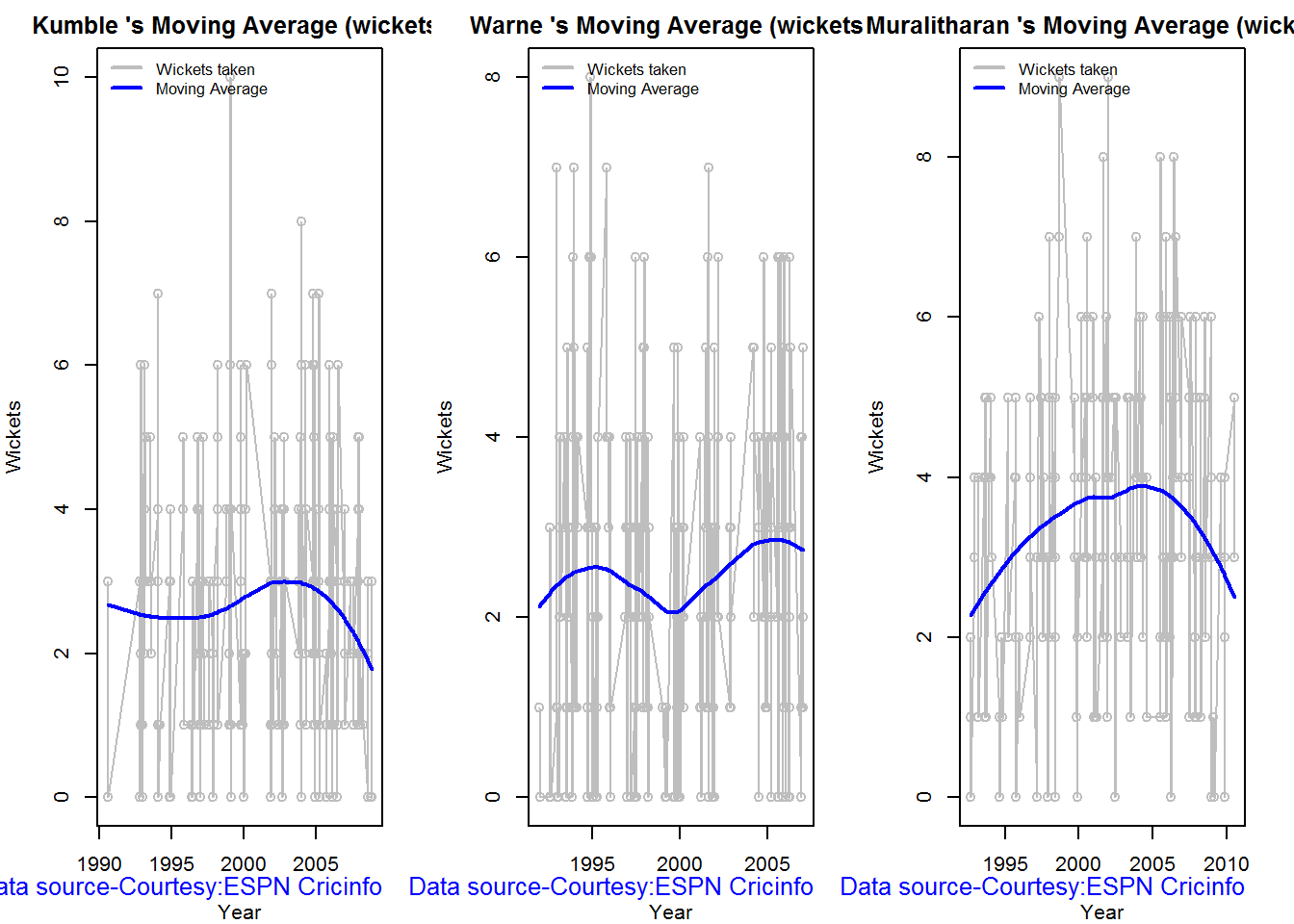
dev.off()## null device
## 1
Future Wickets forecast
Here are plots that forecast how the bowler will perform in future. In this case 90% of the career wickets trend is used as the training set. the remaining 10% is the test set.
A Holt-Winters forecating model is used to forecast future performance based on the 90% training set. The forecated wickets trend is plotted. The test set is also plotted to see how close the forecast and the actual matches
Take a look at the wickets forecasted for the bowlers below. – Shane Warne and Muralitharan have a fairly consistent forecast – Kumble forecast shows a small dip
par(mfrow=c(1,3))
par(mar=c(4,4,2,2))
bowlerPerfForecast("./kumble.csv","Anil Kumble")
bowlerPerfForecast("./warne.csv","Shane Warne")
bowlerPerfForecast("./murali.csv","M Muralitharan")
dev.off()## null device
## 1Contribution to matches won and lost
The plot below is extremely interesting
1. Kumble wickets range from 2 to 4 wickets in matches wons with a mean of 3
2. Warne wickets in won matches range from 1 to 4 with more matches won. Clearly there are other bowlers contributing to the wins, possibly the pacers
3. Muralitharan wickets range in winning matches is more than the other 2 and ranges ranges 3 to 5 and clearly had a hand (pun unintended) in Sri Lanka’s wins
As discussed above the next 2 charts require the use of getPlayerDataSp()
kumblesp par(mfrow=c(1,3))
par(mar=c(4,4,2,2))
bowlerContributionWonLost("kumblesp.csv","Kumble")
bowlerContributionWonLost("warnesp.csv","Warne")
bowlerContributionWonLost("muralisp.csv","Murali")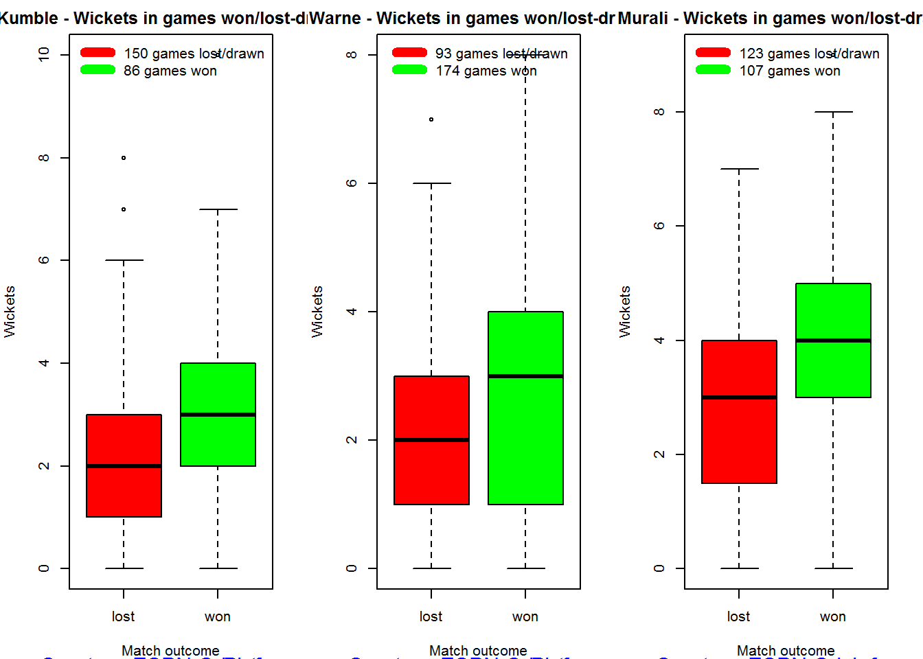
dev.off()## null device
## 1
Performance home and overseas
From the plot below it can be seen that Kumble & Warne have played more matches overseas than Muralitharan. Both Kumble and Warne show an average of 2 wickers overseas, Murali on the other hand has an average of 2.5 wickets overseas but a slightly less number of matches than Kumble & Warne
par(mfrow=c(1,3))
par(mar=c(4,4,2,2))
bowlerPerfHomeAway("kumblesp.csv","Kumble")
bowlerPerfHomeAway("warnesp.csv","Warne")
bowlerPerfHomeAway("muralisp.csv","Murali")
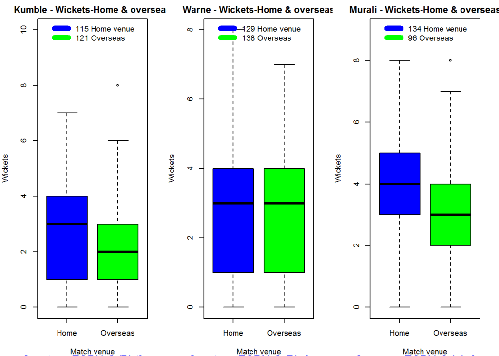

dev.off()## null device
## 1 Check for bowler in-form/out-of-form
The below computation uses Null Hypothesis testing and p-value to determine if the bowler is in-form or out-of-form. For this 90% of the career wickets is chosen as the population and the mean computed. The last 10% is chosen to be the sample set and the sample Mean and the sample Standard Deviation are caculated.
The Null Hypothesis (H0) assumes that the bowler continues to stay in-form where the sample mean is within 95% confidence interval of population mean The Alternative (Ha) assumes that the bowler is out of form the sample mean is beyond the 95% confidence interval of the population mean.
A significance value of 0.05 is chosen and p-value us computed If p-value >= .05 – Batsman In-Form If p-value < 0.05 – Batsman Out-of-Form
Note Ideally the p-value should be done for a population that follows the Normal Distribution. But the runs population is usually left skewed. So some correction may be needed. I will revisit this later
Note: The check for the form status of the bowlers indicate 1. That both Kumble and Muralitharan were out of form. This also shows in the moving average plot 2. Warne is still in great form and could have continued for a few more years. Too bad we didn’t see the magic later
checkBowlerInForm("./kumble.csv","Anil Kumble")## *******************************************************************************************
##
## Population size: 212 Mean of population: 2.69
## Sample size: 24 Mean of sample: 2.04 SD of sample: 1.55
##
## Null hypothesis H0 : Anil Kumble 's sample average is within 95% confidence interval
## of population average
## Alternative hypothesis Ha : Anil Kumble 's sample average is below the 95% confidence
## interval of population average
##
## [1] "Anil Kumble 's Form Status: Out-of-Form because the p value: 0.02549 is less than alpha= 0.05"
## *******************************************************************************************checkBowlerInForm("./warne.csv","Shane Warne")## *******************************************************************************************
##
## Population size: 240 Mean of population: 2.55
## Sample size: 27 Mean of sample: 2.56 SD of sample: 1.8
##
## Null hypothesis H0 : Shane Warne 's sample average is within 95% confidence interval
## of population average
## Alternative hypothesis Ha : Shane Warne 's sample average is below the 95% confidence
## interval of population average
##
## [1] "Shane Warne 's Form Status: In-Form because the p value: 0.511409 is greater than alpha= 0.05"
## *******************************************************************************************checkBowlerInForm("./murali.csv","M Muralitharan")## *******************************************************************************************
##
## Population size: 207 Mean of population: 3.55
## Sample size: 23 Mean of sample: 2.87 SD of sample: 1.74
##
## Null hypothesis H0 : M Muralitharan 's sample average is within 95% confidence interval
## of population average
## Alternative hypothesis Ha : M Muralitharan 's sample average is below the 95% confidence
## interval of population average
##
## [1] "M Muralitharan 's Form Status: Out-of-Form because the p value: 0.036828 is less than alpha= 0.05"
## *******************************************************************************************dev.off()## null device
## 1Key Findings
The plots above capture some of the capabilities and features of my cricketr package. Feel free to install the package and try it out. Please do keep in mind ESPN Cricinfo’s Terms of Use.
Here are the main findings from the analysis above
Analysis of Top 4 batsman
The analysis of the Top 4 test batsman Tendulkar, Kallis, Ponting and Sangakkara show the folliwing
- Sangakkara has the highest average, followed by Tendulkar, Kallis and then Ponting.
- Ponting has the highest strike rate followed by Tendulkar,Sangakkara and then Kallis
- The predicted runs for a given Balls faced and Minutes at crease is highest for Ponting, followed by Tendulkar, Sangakkara and Kallis
- The moving average for Tendulkar and Ponting shows a downward trend while Kallis and Sangakkara retired too soon
- Tendulkar was out of form about the time of retirement while the rest were in-form. But this result has to be taken along with the moving average plot. Ponting was clearly on the way out.
- The home and overseas performance indicate that Tendulkar is the clear leader. He has the highest number of matches played overseas and his performance has been consistent. He is followed by Ponting, Kallis and finally Sangakkara
Analysis of Top 3 legs spinners
The analysis of Anil Kumble, Shane Warne and M Muralitharan show the following
- Muralitharan has the highest wickets and best economy rate followed by Warne and Kumble
- Muralitharan has higher wickets frequency percentage between 3 to 8 wickets
- Muralitharan has the best Economy Rate for wickets between 2 to 7
- The moving average plot shows that the time was up for Kumble and Muralitharan but Warne had a few years ahead
- The check for form status shows that Muralitharan and Kumble time was over while Warne still in great form
- Kumble’s has more matches abroad than the other 2, yet Kumble averages of 3 wickets at home and 2 wickets overseas liek Warne . Murali has played few matches but has an average of 4 wickets at home and 3 wickets overseas.
Final thoughts
Here are my final thoughts
Batting
Among the 4 batsman Tendulkar, Kallis, Ponting and Sangakkara the clear leader is Tendulkar for the following reasons
- Tendulkar has the highest test centuries and runs of all time.Tendulkar’s average is 2nd to Sangakkara, Tendulkar’s predicted runs for a given Balls faced and Minutes at Crease is 2nd and is behind Ponting. Also Tendulkar’s performance at home and overseas are consistent throughtout despite the fact that he has a highest number of overseas matches
- Ponting takes the 2nd spot with the 2nd highest number of centuries, 1st in Strike Rate and 2nd in home and away performance.
- The 3rd spot goes to Sangakkara, with the highest average, 3rd highest number of centuries, reasonable run frequency percentage in different run ranges. However he has a fewer number of matches overseas and his performance overseas is significantly lower than at home
- Kallis has the 2nd highest number of centuries but his performance overseas and strike rate are behind others
- Finally Kallis and Sangakkara had a few good years of batting still left in them (pity they retired!) while Tendulkar and Ponting’s time was up
Bowling
Muralitharan leads the way followed closely by Warne and finally Kumble. The reasons are
- Muralitharan has the highest number of test wickets with the best Wickets percentage and the best Economy Rate. Murali on average gas taken 4 wickets at home and 3 wickets overseas
- Warne follows Murali in the highest wickets taken, however Warne has less matches overseas than Murali and average 3 wickets home and 2 wickets overseas
- Kumble has the 3rd highest wickets, with 3 wickets on an average at home and 2 wickets overseas. However Kumble has played more matches overseas than the other two. In that respect his performance is great. Also Kumble has played less matches at home otherwise his numbers would have looked even better.
- Also while Kumble and Muralitharan’s career was on the decline , Warne was going great and had a couple of years ahead.
You can download this analysis at Introducing cricketr
Hope you have fun using the cricketr package as I had in developing it. Do take a look at my follow up post Taking cricketr for a spin – Part 1
Important note: Do check out my other posts using cricketr at cricketr-posts
Do take a look at my 2nd package “The making of cricket package yorkr – Part 1”
Also see
1. My book “Deep Learning from first principles” now on Amazon
2. My book ‘Practical Machine Learning with R and Python’ on Amazon
3. Taking cricketr for a spin – Part 1
4. cricketr plays the ODIs
5. cricketr adapts to the Twenty20 International
6. Analyzing cricket’s batting legends – Through the mirage with R
7. Masters of spin: Unraveling the web with R
8. Mirror,mirror …best batsman of them all
You may also like
1. A crime map of India in R: Crimes against women
2. What’s up Watson? Using IBM Watson’s QAAPI with Bluemix, NodeExpress – Part 1
3. Bend it like Bluemix, MongoDB with autoscaling – Part 2
4. Informed choices through Machine Learning : Analyzing Kohli, Tendulkar and Dravid
5. Thinking Web Scale (TWS-3): Map-Reduce – Bring compute to data
6. Deblurring with OpenCV:Weiner filter reloaded
7. Fun simulation of a Chain in Androidhttp://www.r-bloggers.com/introducing-cricketr-an-r-package-to-analyze-performances-of-cricketers/
Share:

A crime map of India in R – Crimes against women
In this post I take a look at the gory crime scene across India to determine which states are the heavy weights in crimes. Who is the undisputed champion of rapes in a year? Which state excels in cruelty by husbands and the relatives to wives? Which state leads in dowry deaths? To get the answers to these questions I perform analysis of the state-wise crime data against women with the data from Open Government Data (OGD) Platform India. The dataset for this analysis was taken for the Crime against Women from OGD.
(Do see my post Revisiting crimes against women in India which includes an interactive Shiny app)
The data in OGD is available for crimes against women in different states under different ‘crime heads’ like rape, dowry deaths, kidnapping & abduction etc. The data is available for years from 2001 to 2012. This data is plotted as a scatter plot and a linear regression line is then fit on the available data. Based on this linear model, the projected incidence of crimes likes rapes, dowry deaths, abduction & kidnapping is performed for each of the states. This is then used to build a table of different crime heads for all the states predicting the number of crimes till the year 2018. Fortunately, R crunches through the data sets quite easily. The overall projections of crimes against as women is shown below based on the linear regression for each of these states
Projections over the next couple of years
The tables below are based on the projected incidence of crimes under various categories assuming that these states maintain their torrid crime rate. A cursory look at the tables below clearly indicate the Uttar Pradesh is the undisputed heavy weight champion in 4 of 5 categories shown. Maharashtra and Andhra Pradesh take 2nd and 3rd ranks in the total crimes against women and are significant contenders in other categories too.
A) Projected rapes in India
The top 3 heavy weights in projected rapes over the next 5 years are 1) Madhya Pradesh 2) Uttar Pradesh 3) Maharashtra

Full table: Rape.csv
B) Projected Dowry deaths in India
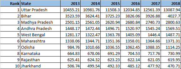
Full table: Dowry Deaths.csv
C) Kidnapping & Abduction

Full table: Kidnapping&Abduction.csv
D) Cruelty by husband & relatives

Full table: Cruelty by husbands_relatives.csv
E) Total crimes against women
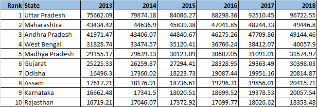
Full table: Total crimes.csv
Here is a visualization of ‘Total crimes against women’ created as a choropleth map
 The implementation for this analysis was done using the R language. The R code, dataset, output and the crime charts can be accessed at GitHub at crime-against-women
Directory structure
– R code
– dataset used
– output
– statewise-crime-charts
The analysis has been completely parametrized. A quick look at the implementation is shown below. A function state crime was created as given below
statecrime.R
This function (statecrime.R) does the following
a) Creates a scatter plot for the state for the crime head
b) Computes a best linear regression fir and draws this line
c) Uses the model parameters (coefficients) to compute the projected crime in the years to come
d) Writes the projected values to a text file
c) Creates a directory with the name of the state if it does not exist and stores the jpeg of the plot there.
statecrime <- function(indiacrime, row, state,crime) {

year <- c(2001:2012)

# Make seperate folders for each state

if(!file.exists(state)) {

dir.create(state)

}

setwd(state)

crimeplot <- paste(crime,".jpg")

jpeg(crimeplot)
# Plot the details of the crime
plot(year,thecrime ,pch= 15, col="red", xlab = "Year", ylab= crime, main = atitle,

,xlim=c(2001,2018),ylim=c(ymin,ymax), axes=FALSE)
A linear regression line is fit using ‘lm’
# Fit a linear regression model

lmfit <-lm(thecrime~year)

# Draw the lmfit line

abline(lmfit)
The model parameters are then used to draw the line and also project for the next 5 years from 2013 to 2018
nyears <-c(2013:2018)

nthecrime <- rep(0,length(nyears))

# Projected crime incidents from 2013 to 2018 using a linear regression model

for (i in seq_along(nyears)) {

nthecrime[i] <- lmfit$coefficients[2] * nyears[i] + lmfit$coefficients[1]

}
The projected data for each state is appended into an appropriate file which is then used to display the tables at the top of this post
# Write the projected crime rate in a file
nthecrime <- round(nthecrime,2)

nthecrime <- c(state, nthecrime, "\n")

print(nthecrime)

#write(nthecrime,file=fileconn, ncolumns=9, append=TRUE,sep="\t")

filename <- paste(crime,".txt")

# Write the output in the ./output directory

setwd("./output")

cat(nthecrime, file=filename, sep=",",append=TRUE)
The above function is then repeatedly called for each state for the different crime heads. (Note: It is possible to check the read both the states and crime heads with R and perform the computation repeatedly. However, I have done this the manual way!)
crimereport.R
# 1. Andhra Pradesh

i <- 1

statecrime(indiacrime, i, "Andhra Pradesh","Rape")

i <- i+38

statecrime(indiacrime, i, "Andhra Pradesh","Kidnapping& Abduction")

i <- i+38

statecrime(indiacrime, i, "Andhra Pradesh","Dowry Deaths")

i <- i+38

statecrime(indiacrime, i, "Andhra Pradesh","Assault on Women")

i <- i+38

statecrime(indiacrime, i, "Andhra Pradesh","Insult to modesty")

i <- i+38

statecrime(indiacrime, i, "Andhra Pradesh","Cruelty by husband_relatives")

i <- i+38

statecrime(indiacrime, i, "Andhra Pradesh","Imporation of girls from foreign country")

i <- i+38

statecrime(indiacrime, i, "Andhra Pradesh","Immoral traffic act")

i <- i+38

statecrime(indiacrime, i, "Andhra Pradesh","Dowry prohibition act")

i <- i+38

statecrime(indiacrime, i, "Andhra Pradesh","Indecent representation of Women Act")

i <- i+38

statecrime(indiacrime, i, "Andhra Pradesh","Commission of Sati Act")

i <- i+38

statecrime(indiacrime, i, "Andhra Pradesh","Total crimes against women")

...

...
and so on for all the states
Charts for different crimes against women
1) Uttar Pradesh
The plots for Uttar Pradesh are shown below
Rapes in UP

Dowry deaths in UP
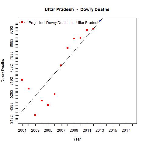
Cruelty by husband/relative

Total crimes against women in Uttar Pradesh

You can find more charts in GitHub by clicking Uttar Pradesh
2) Maharashtra : Some of the charts for Maharashtra
Rape

Kidnapping & Abduction

Total crimes against women in Maharashtra

More crime charts for Maharashtra
Crime charts can be accessed for the following states from GitHub ( in alphabetical order)
3) Andhra Pradesh
4) Arunachal Pradesh
5) Assam
6) Bihar
7) Chattisgarh
8) Delhi (Added as an exception based on its notoriety)
9) Goa
10) Gujarat
11) Haryana
12) Himachal Pradesh
13) Jammu & Kashmir
14) Jharkhand
15) Karnataka
16) Kerala
17) Madhya Pradesh
18) Manipur
19) Meghalaya
20) Mizoram
21) Nagaland
22) Odisha
23) Punjab
24) Rajasthan
25) Sikkim
26) Tamil Nadu
27) Tripura
28) Uttarkhand
29) West Bengal
The code, dataset and the charts can be cloned/forked from GitHub at crime-against-women
Let me know if you find any interesting patterns in the data.
Thoughts, comments welcome!
See also
My book ‘Practical Machine Learning with R and Python’ on Amazon
A peek into literacy in India: Statiscal learning with R
You may also like
– Analyzing cricket’s batting legends – Through the mirage with R
– What’s up Watson? Using IBM Watson’s QAAPI with Bluemix, NodeExpress – Part 1
– Bend it like Bluemix, MongoDB with autoscaling – Part 1
Share:

Applying the principles of Machine Learning
While working with multivariate regression there are certain essential principles that must be applied to ensure the correctness of the solution while being able to pick the most optimum solution. This is all the more important when the problem has a large number of features. In this post I apply these important principles to a regression data set which I was able to pull of the internet. This data set was taken from the UCI Machine Learning repository and deals with Boston housing data. The housing data provides the cost of house in Boston suburbs given the number of rooms, the connectivity to main highways, and crime rate in the area and several other data. There are a total of 506 data points in this data set with a total of 13 features.
This seemed a reasonable dataset to start to try out the principles of Machine Learning I had picked up from Coursera’s ML course.
Out of a total of 13 features 2 features ’ZN’ and ‘CHAS’ proximity to Charles river were dropped as the values were mostly zero in these columns . The remaining 11 features were used to map to the output variable of the price.
The following key rules have been applied on the
- The dataset was divided into training samples (60%), cross-validation set (20%) and test set (20%) using a random index
- Try out different polynomial functions while performing gradient descent to determine the theta values
- Different combinations of ‘alpha’ learning rate and ‘lambda’ the regularization parameter were tried while performing gradient descent
- The error rate is then calculated on the cross-validation and test set
- The theta values that were obtained for the lowest cost for a polynomial was used to compute and plot the learning curve for the different polynomials against increasing number of training and cross-validation test samples to check for bias and variance.
- The plot of the cost versus the polynomial degree was plotted to obtain the best fit polynomial for the data set.
A multivariate regression hypothesis can be represented as
hθ(x) = θ0 + θ1x1 + θ2x2 + θ3x3 + θ4x4 + …
And the cost can is determined as
J(θ0, θ1, θ2, θ3..) = 1/2m ∑ (hΘ (xi) -yi)2
The implementation was done using Octave. As in my previous posts some functions have not been include to comply with Coursera’s Honor Code. The code can be cloned from GitHub at machine-learning-principles
a) housing compute.m. In this module I perform gradient descent for different polynomial degrees and check the error that is obtained when using the computed theta on the cross validation and test set
max_degrees =4;

J_history = zeros(max_degrees, 1);

Jcv_history = zeros(max_degrees, 1);

for degree = 1:max_degrees;

[J Jcv alpha lambda] = train_samples(randidx, training,cross_validation,test_data,degree);

end;
b) train_samples.m – This module uses gradient descent to check the best fit for a given polynomial degree for different combinations of alpha (learning rate) and lambda( regularization).
for i = 1:length(alpha_arr),

for j = 1:length(lambda_arr)

alpha = alpha_arr{i};

lambda= lambda_arr{j};

% Perform Gradient descent

% Compute error for training sample for computed theta values

% Compute the error rate for the cross validation samples

% Compute the error rate against the test set

end;

end;
c) cross_validation.m – This module uses the theta values to compute cost for the cross validation set
d) test-samples.m – This modules computes the error when using the trained theta on the test set
e) poly.m – This module constructs polynomial vectors based on the degree as follows
function [x] = poly(xinput, n)

x = [];

for i= 1:n

xtemp = xinput .^i;

x = [x xtemp];

end;
e) learning_curve.m – The learning curve module plots the error rate for increasing number of training and cross validation samples. This is done as follows. For the theta with the lowest cost as determined by gradient descent
for i from 1 to 100
- Compute the error for ‘i’ training samples
- Compute the error for ‘i’ cross-validation
- Plot the learning curve to determine the bias and variance of the polynomial fit
This is included below
for i = 1: 100

xsample = xtrain(1:i,:);

ysample = ytrain(1:i,:);

size(xsample);

size(ysample);

[xsample] = poly(xsample,degree);

xsample= [ones(i, 1) xsample];

[c d] = size(xsample);

theta = zeros(d, 1);

% Minimize using fmincg

J = computeCost(xsample, ysample, theta);

Jtrain(i) = J;

xsample_cv = xcv(1:i,:);

ysample_cv = ycv(1:i,:);

[xsample_cv] = poly(xsample_cv,degree);

xsample_cv= [ones(i, 1) xsample_cv];

J_cv = computeCost(xsample_cv, ysample_cv,theta)

Jcv(i) = J_cv;

end;
Finally a plot is done been different lambda and the cost.
The results are included below
A) Polynomial degree 1
Convergence graph

Learning curve

The above figure does show a stronger bias. Note: the learning curve was done with around 100 samples
B) Polynomial degree 2
Convergence graph
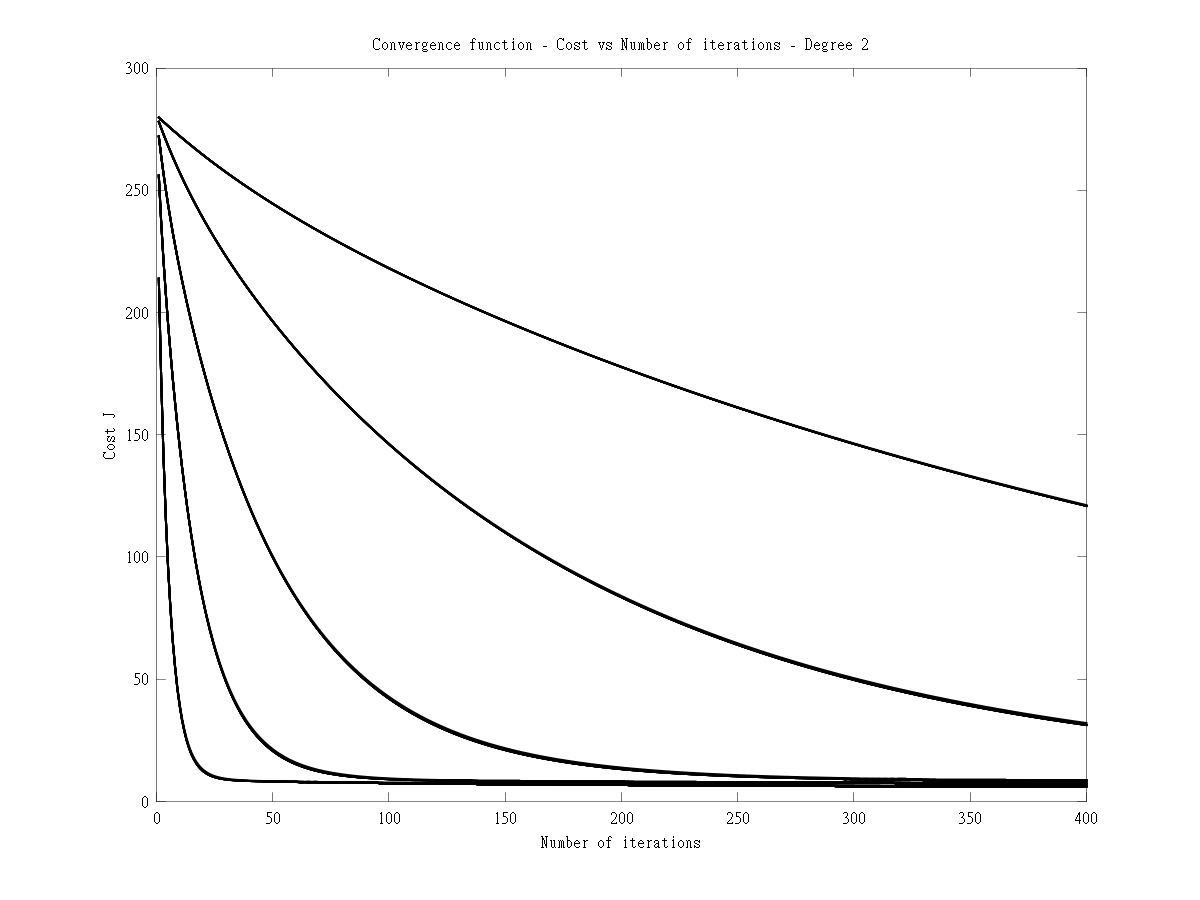
Learning curve

The learning curve for degree 2 shows a stronger variance.
C) Polynomial degree 3
Convergence graph

Learning curve

D) Polynomial degree 4
Convergence graph
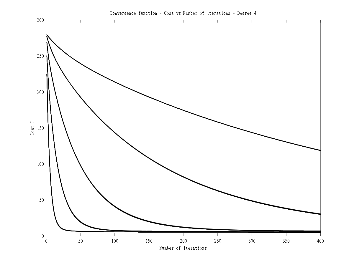
E) Learning curve

This plot is useful to determine which polynomial degree will give the best fit for the dataset and the lowest cost
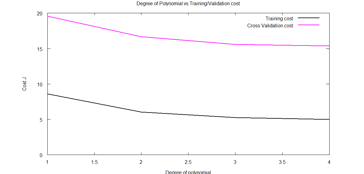
Clearly from the above it can be seen that degree 2 will give a good fit for the data set.
F) Lambda vs Cost function

The above code demonstrates some key principles while performing multivariate regression
The code can be cloned from GitHub at machine-learning-principles
Share:

Informed choices through Machine Learning – Analyzing Kohli, Tendulkar and Dravid
Having just completed the highly stimulating & inspiring Stanford’s Machine Learning course at Coursera, by the incomparable Professor Andrew Ng I wanted to give my newly acquired knowledge a try. As a start, I decided to try my hand at analyzing one of India’s fastest growing stars, namely Virat Kohli . For the data on Virat Kohli I used the ‘Statistics database’ at ESPN Cricinfo. To make matters more interesting, I also pulled data on the iconic Sachin Tendulkar and the Mr. Dependable, Rahul Dravid.
If you are passionate about cricket, and love analyzing cricket performances, then check out my 2 racy books on cricket! In my books, I perform detailed yet compact analysis of performances of both batsmen, bowlers besides evaluating team & match performances in Tests , ODIs, T20s & IPL. You can buy my books on cricket from Amazon at $12.99 for the paperback and $4.99/$6.99 respectively for the kindle versions. The books can be accessed at Cricket analytics with cricketr and Beaten by sheer pace-Cricket analytics with yorkr A must read for any cricket lover! Check it out!!
(Also do check out my R package cricketr Introducing cricketr! : An R package to analyze performances of cricketers and my interactive Shiny app implementation using my R package cricketr – Sixer – R package cricketr’s new Shiny avatar )
Based on the data of these batsmen I perform some predictions with the help of machine learning algorithms. That I have a proclivity for prediction, is not surprising, considering the fact that my Dad was an astrologer who had reasonable success at this esoteric art. While he would be concerned with planetary positions, about Rahu in the 7th house being in the malefic etc., I on the other hand focus my predictions on multivariate regression analysis and K-Means. The first part of my post gives the results of my analysis and some predictions for Kohli, Tendulkar and Dravid.
The second part of the post contains a brief outline of the implementation and not the actual details of implementation. This is ensure that I don’t violate Coursera’s Machine Learning’ Honor Code.
This code, data used and the output obtained can be accessed at GitHub at ml-cricket-analysis
Analysis and prediction of Kohli, Tendulkar and Dravid with Machine Learning As mentioned above, I pulled the data for the 3 cricketers Virat Kohli, Sachin Tendulkar and Rahul Dravid. The data taken from Cricinfo database for the 3 batsman is based on the following assumptions
- Only ‘Minutes at Crease’ and ‘Balls Faced’ were taken as features against the output variable ‘Runs scored’
- Only test matches were taken. This included both test ‘at home’ and ‘away tests’
- The data was cleaned to remove any DNB (did not bat) values
- No extra weightage was given to ‘not out’. So if Kohli made ‘28*’ 28 not out, this was taken to be 28 runs
Regression Analysis for Virat Kohli There are 51 data points for Virat Kohli regarding Tests played. The data for Kohli is displayed as a 3D scatter plot where x-axis is ‘minutes’ and y-axis is ‘balls faced’. The vertical z-axis is the ‘runs scored’. Multivariate regression analysis was performed to find the best fitting plane for the runs scored based on the selected features of ‘minutes’ and ‘balls faced’.
This is based on minimizing the cost function and then performing gradient descent for 400 iterations to check for convergence. This plane is shown as the 3-D plane that provides the best fit for the data points for Kohli. The diagram below shows the prediction plane of expected runs for a combination of ‘minutes at crease’ and ‘balls faced’. Here are 2 such plots for Virat Kohli.  Another view of the prediction plane
  Prediction for Kohli I have also computed the predicted runs that will be scored by Kohli for different combinations of ‘minutes at crease’ and ‘balls faced’. As an example, from the table below, we can see that the predicted runs for Kohli after being in the crease for 110 minutes and facing 135 balls is 54 runs.
  Regression analysis for Sachin Tendulkar There was a lot more data on Tendulkar and I was able to dump close to 329 data points. As before the ‘minutes at crease’, ‘balls faced’ vs ‘runs scored’ were plotted as a 3D scatter plot. The prediction plane is calculated using gradient descent and is shown as a plane in the diagram below
  Another view of this below
  Predicted runs for Tendulkar The table below gives the predicted runs for Tendulkar for a combination of time at crease and balls faced. Hence, Tendulkar will score 57 runs in 110 minutes after facing 135 deliveries
  Regression Analysis for Rahul Dravid The same was done for ‘the Wall’ Dravid. The prediction plane is below
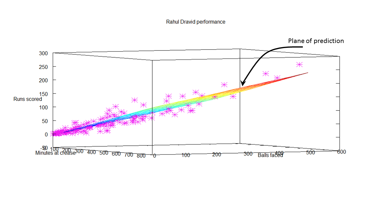 Predicted runs for Dravid The predicted runs for Dravid for combinations of batting time and balls faced is included below. The predicted runs for Dravid after facing 135 deliveries in 110 minutes is 44.
  Further analysis While the ‘prediction plane’ was useful, it somehow does not give a clear picture of how effective each batsman is. Clearly the 3D plots show at least 3 clusters for each batsman. For all batsmen, the clustering is densest near the origin, become less dense towards the middle and sparse on the other end. This is an indication during which session during their innings the batsman is most prone to get out. So I decided to perform K-Means clustering on the data for the 3 batsman. This gives the 3 general tendencies for each batsman. The output is included below
K-Means for Virat The K-Means for Virat Kohli indicate the follow
Centroids found 255.000000 104.478261 19.900000
Centroids found 194.000000 80.000000 15.650000
Centroids found 103.000000 38.739130 7.000000
Analysis of Virat Kohli’s batting tendency
Kohli has a 45.098 percent tendency to bat for 104 minutes, face 80 balls and score 38 runs
Kohli has a 39.216 percent tendency to bat for 19 minutes, face 15 balls and score 7 runs
Kohli has a 15.686 percent tendency to bat for 255 minutes, face 194 balls and score 103 runs
The computation of this included in the diagram below

K-means for Sachin Tendulkar
The K-Means for Sachin Tendulkar indicate the following
Centroids found 166.132530 353.092593 43.748691
Centroids found 121.421687 250.666667 30.486911
Centroids found 65.180723 138.740741 15.748691
Analysis of Sachin Tendulkar’s performance
Tendulkar has a 58.232 percent tendency to bat for 43 minutes, face 30 balls and score 15 runs
Tendulkar has a 25.305 percent tendency to bat for 166 minutes, face 121 balls and score 65 runs
Tendulkar has a 16.463 percent tendency to bat for 353 minutes, face 250 balls and score 138 runs
 K-Means for Rahul Dravid
Centroids found 191.836364 409.000000 50.506024
Centroids found 137.381818 290.692308 34.493976
Centroids found 56.945455 131.500000 13.445783
Analysis of Rahul Dravid’s performance
Dravid has a 50.610 percent tendency to bat for 50 minutes, face 34 balls and score 13 runs
Dravid has a 33.537 percent tendency to bat for 191 minutes, face 137 balls and score 56 runs
Dravid has a 15.854 percent tendency to bat for 409 minutes, face 290 balls and score 131 runs
 Some implementation details The entire analysis and coding was done with Octave 3.2.4. I have included the outline of the code for performing the multivariate regression. In essence the pseudo code for this
- Read the batsman data (Minutes, balls faced versus Runs scored)
- Calculate the cost
- Perform Gradient descent
The cost was plotted against the number of iterations to ensure convergence while performing gradient descent  Plot the 3-D plane that best fits the data
The outline of this code, data used and the output obtained can be accessed at GitHub at ml-cricket-analysis
Conclusion: Comparing the results from the K-Means Tendulkar has around 48% to make a score greater than 60
Tendulkar has a 25.305 percent tendency to bat for 166 minutes, face 121 balls and score 65 runs
Tendulkar has a 16.463 percent tendency to bat for 353 minutes, face 250 balls and score 138 runs
And Dravid has a similar 48% tendency to score greater than 56 runs
Dravid has a 33.537 percent tendency to bat for 191 minutes, face 137 balls and score 56 runs
Dravid has a 15.854 percent tendency to bat for 409 minutes, face 290 balls and score 131 runs
Kohli has around 45% to score greater than 38 runs
Kohli has a 45.098 percent tendency to bat for 104 minutes, face 80 balls and score 38 runs
Also Kohli has a lesser percentage to score lower runs as against the other two
Kohli has a 39.216 percent tendency to bat for 19 minutes, face 15 balls and score 7 runs
The results must be looked in proper perspective as Kohli is just starting his career while the other 2 are veterans. Kohli has a long way to go and I am certain that he will blaze a trail of glory in the years to come!
Watch this space!
Also see
1. My book ‘Practical Machine Learning with R and Python’ on Amazon
2.Introducing cricketr! : An R package to analyze performances of cricketers
3.Informed choices with Machine Learning 2 – Pitting together Kumble, Kapil and Chandra
4. Analyzing cricket’s batting legends – Through the mirage with R
5. What’s up Watson? Using IBM Watson’s QAAPI with Bluemix, NodeExpress – Part 1
6. Bend it like Bluemix, MongoDB with autoscaling – Part 1
Share:

Simplifying ML: Recommender Systems – Part 7
In this age of Amazon, Netflix and App stores where products, movies and apps are purchased online the method of up-selling and cross-selling online is through the use of recommender based systems.
When you go to site like Amazon/Flipkart or purchase apps on App store/Google Play we often see things like “People who bought this book/app also bought X, Y, Z”. These recommendations are the recommender system algorithms in action.
Recently, Netflix ran a competition in which users had to come with the best algorithm to recommend films that a user would also like. The prize money for this was of the order of $1 million. That’s how critical recommender systems are to organizations of today where most of the transactions happen on the web.
Typically users are asked to give a rating of 1 to 5 with 1 being the lowest and 5 being the highest. So for example if we had classics like Moby Dick, Great Expectations and current best sellers like The Client, The da Vinci Code and a Science Fiction like 2001- A Space Odyssey we can expect that different people will rate the books differently. Obviously not everybody would have read every book in the list and some elements would be blank.

Recommender Systems are based on machine learning algorithms. The goal of these algorithms is to predict what score any user would give to books they did not rate. In other words what would be rating the buyers would give for books or apps they did not buy. So if the algorithm predicts a high rating then we could recommend that the user would also ‘like’ them. Or we could give recommendations of books/apps bought by users who bought the books/apps bought by this user.
The notation is
nu = Number of users
nb = Number of books
r(i,j) = Boolean whether user j rated a book i
y(i,j) = The rating user j gave book i
mj = The number of books that user j rated
Content based recommendation
In a typical content based recommendation algorithm we assume that we have data about some items we want to recommend rating for e.g. books/products/apps. In the example for books bought in an online bookstore we assume some features in our case ‘classic’, “fiction” etc

So each book has its own feature vector where x1 is the feature vector of the first book x2 feature vector of the 2nd book and so on
This can be done through linear regression by minimizing the cost function of the sum of squared errors from the predicted value
So for a parameter vector Ɵjand a feature vector xi the recommender system will try to predict the rating that a user j will give a book i.
This can be written as
Number of stars (rating) = (θj) T xi
This reduces to the minimization problem over all θj for r=1
min 1/2m Σ ((θj)T xi – y i,j)2
θj i:r=1
Adding the regularization term this becomes
min 1/2m Σ((θj)T xi – y i,j)2 + λ/2m(Σ θj)2
θj i:r=1
The recommender algorithm in essence tries to learn parameters θj for a set of features of xi the chosen system for e.g. books in this case.
The recommender tries to learn the parameters for all the users
min 1/2m Σ Σ((θj)T xi – y i,j)2 + λ/2m(Σ Σ θj)2
θ1…θn i:r=1
The minimization is performed by gradient descent as
Θj k:= Θjk – α (Σ((θj)T xi – y i,j)xi + λ Θj k
Recommender systems tries to learn the parameters for a set of chosen features over all users. Based on the learnt paramaters it then tries to predict the rating the user would give to books/apps that he is yet to purchase and push up those apps for which the user is likely to give a high rating based on the given set of ratings.
Recommender systems contribute substantially to the revenues of e-commerce sites like Amazon, Flipkart, Netflix etc
Note: This post, line previous posts on Machine Learning, is based on the Coursera course on Machine Learning by Professor Andrew Ng
Find me on Google+
Share:

Simplifying ML: Impact of degree of polynomial degree on bias & variance and other insights
This post takes off from my earlier post Simplifying Machine Learning: Bias, variance, regularization and odd facts- Part 4. As discussed earlier a poor hypothesis function could either underfit or overfit the data. If the number of features selected were small of the order of 1 or 2 features, then we could plot the data and try to determine how the hypothesis function fits the data. We could also see whether the function is capable of predicting output target values for new data.
However if the number of features were large for e.g. of the order of 10’s of features then there needs to be method by which one can determine if the learned hypotheses is a ‘just right’ fit for all the data.
Checkout my book ‘Deep Learning from first principles Second Edition- In vectorized Python, R and Octave’. My book is available on Amazon as paperback ($18.99) and in kindle version($9.99/Rs449).
You may also like my companion book “Practical Machine Learning with R and Python:Second Edition- Machine Learning in stereo” available in Amazon in paperback($12.99) and Kindle($9.99/Rs449) versions.
The following technique can be used to determine the ‘goodness’ of a hypothesis or how well the hypothesis can fit the data and can also generalize to new examples not in the training set.
Several insights on how to evaluate a hypothesis is given below
Consider a hypothesis function
hƟ (x) = Ɵ0 + Ɵ1x1 + Ɵ2x22 + Ɵ3x33 + Ɵ4x44

The above hypothesis does not generalize well enough for new examples in the data set.
Let us assume that there 100 training examples or data sets. Instead of using the entire set of 100 examples to learn the hypothesis function, the data set is divided into training set and test set in a 70%:30% ratio respectively
The hypothesis is learned from the training set. The learned hypothesis is then checked against the 30% test set data to determine whether the hypothesis is able to generalize on the test set also.
This is done by determining the error when the hypothesis is used against the test set.
For linear regression the error is computed by determining the average mean square error of the output value against the actual value as follows
The test set error is computed as follows
Jtest(Ɵ) = 1/2mtest Σ(hƟ (xtesti – ytesti)2
For logistic regression the test set error is similarly determined as
Jtest(Ɵ) = = 1/mtest Σ -ytest * log(hƟ (xtest)) – (1-ytest) * (log(1 – hƟ (xtest))
The idea is that the test set error should as low as possible.
Model selection
A typical problem in determining the hypothesis is to choose the degree of the polynomial or to choose an appropriate model for the hypothesis
The method that can be followed is to choose 10 polynomial models
- hƟ (x) = Ɵ0 + Ɵ1x1
- hƟ (x) = Ɵ0 + Ɵ1x1 + Ɵ2x22
- hƟ (x) = Ɵ0 + Ɵ1x12 + Ɵ2x22 + Ɵ3x33
- …
Here‘d’ is the degree of the polynomial. One method is to train all the 10 models. Run each of the model’s hypotheses against the test set and then choose the model with the smallest error cost.
While this appears to a good technique to choose the best fit hypothesis, in reality it is not so. The reason is that the hypothesis chosen is based on the best fit and the least error for the test data. However this does not generalize well for examples not in the training or test set.
So the correct method is to divide the data into 3 sets as 60:20:20 where 60% is the training set, 20% is used as a test set to determine the best fit and the remaining 20% is the cross-validation set.
The steps carried out against the data is
- Train all 10 models against the training set (60%)
- Compute the cost value J against the cross-validation set (20%)
- Determine the lowest cost model
- Use this model against the test set and determine the generalization error.
Degree of the polynomial versus bias and variance
How does the degree of the polynomial affect the bias and variance of a hypothesis?
Clearly for a given training set when the degree is low the hypothesis will underfit the data and there will be a high bias error. However when the degree of the polynomial is high then the fit will get better and better on the training set (Note: This does not imply a good generalization)
We run all the models with different polynomial degrees on the cross validation set. What we will observe is that when the degree of the polynomial is low then the error will be high. This error will decrease as the degree of the polynomial increases as we will tend to get a better fit. However the error will again increase as higher degree polynomials that overfit the training set will be a poor fit for the cross validation set.
This is shown below

Effect of regularization on bias & variance
Here is the technique to choose the optimum value for the regularization parameter λ
When λ is small then Ɵi values are large and we tend to overfit the data set. Hence the training error will be low but the cross validation error will be high. However when λ is large then the values of Ɵi become negligible almost leading to a polynomial degree of 1. These will underfit the data and result in a high training error and a cross validation error. Hence the chosen value of λ should be such that the cross validation error is the lowest

Plotting learning curves
This is another technique to identify if the learned hypothesis has a high bias or a high variance based on the number of training examples
A high bias indicates an underfit. When the number of samples in training set if low then the training error and cross validation error will be low as it will be easy to create a hypothesis if there are few training examples. As the number of samples increase the error will increase for the training set and will slightly decrease for the cross validation set. However for a high bias, or underfit, after a certain point increasing the number of samples will not change the error. This is the case of a high bias

In the case of high variance where a high degree polynomial is used for the hypothesis the training error will be low for smaller number of training examples. As the number of training examples increase the error will increase slowly. The cross validation error will be high for lesser number of training samples but will slowly decrease as the number of samples grow as the hypothesis will learn better. Hence for the case of high variance increasing the number of samples in the training set size will decrease the gap between the cross validation and the training error as shown below
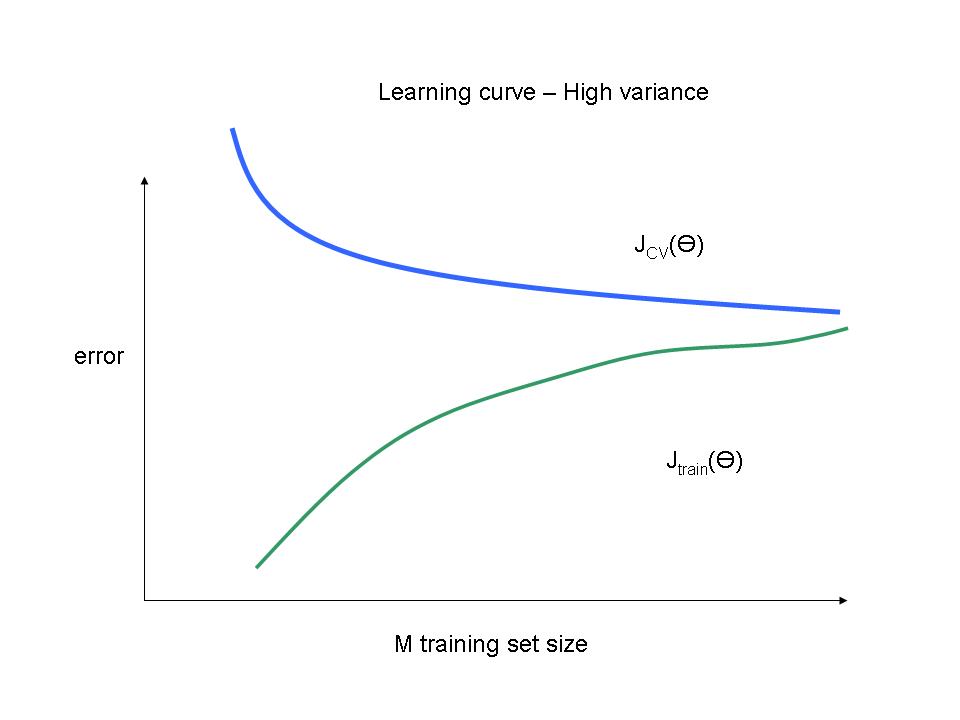
Note: This post, line previous posts on Machine Learning, is based on the Coursera course on Machine Learning by Professor Andrew Ng
Also see
1. My book ‘Practical Machine Learning in R and Python: Third edition’ on Amazon
2.My book ‘Deep Learning from first principles:Second Edition’ now on Amazon
3.The Clash of the Titans in Test and ODI cricket
4. Introducing QCSimulator: A 5-qubit quantum computing simulator in R
5.Latency, throughput implications for the Cloud
6. Simulating a Web Joint in Android
5. Pitching yorkpy … short of good length to IPL – Part 1


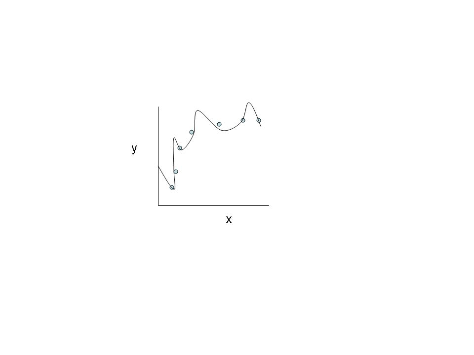