Continuing my earlier ‘innings’, of test driving my knowledge in Machine Learning acquired via Coursera, I now turn my attention towards the bowling performances of our Indian bowling heroes. In this post I give a slightly different ‘spin’ to the bowling analysis and hope I can ‘swing’ your opinion based on my assessment.
I guess that is enough of my cricketing ‘double-speak’ for now and I will get down to the real business of my bowling analysis!
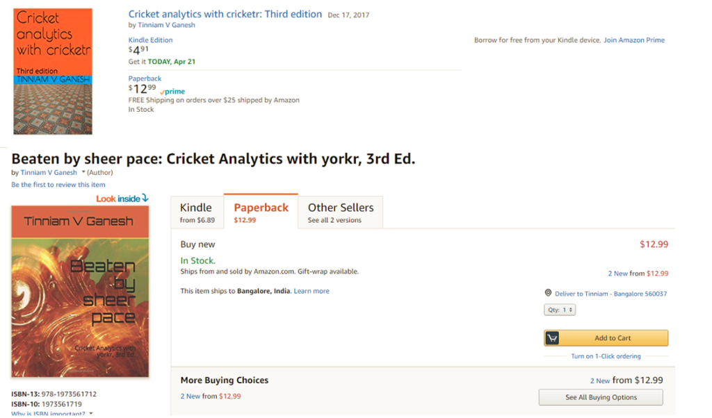
If you are passionate about cricket, and love analyzing cricket performances, then check out my 2 racy books on cricket! In my books, I perform detailed yet compact analysis of performances of both batsmen, bowlers besides evaluating team & match performances in Tests , ODIs, T20s & IPL. You can buy my books on cricket from Amazon at $12.99 for the paperback and $4.99/$6.99 respectively for the kindle versions. The books can be accessed at Cricket analytics with cricketr and Beaten by sheer pace-Cricket analytics with yorkr A must read for any cricket lover! Check it out!!
As in my earlier post Informed choices through Machine Learning – Analyzing Kohli, Tendulkar and Dravid ,the first part of the post has my analyses and the latter part has the details of the implementation of the algorithm. Feel free to read the first part and either scan or skip the latter.
To perform this analysis I have skipped the data on our recent crop of new bowlers. The reason being that data is scant on these bowlers, besides they also seem to have a relatively shorter shelf life (hope there are a couple of finds in this Australian tour of Dec 2014). For the analyses I have chosen B S Chandrasekhar, Kapil Dev Anil Kumble. My rationale as to why I chose the above 3
B S Chandrasekhar also known as “Chandra’ was one of the most lethal leg spinners in the late 1970’s. He had a very dangerous combination of fast leg breaks, searing tops spins interspersed with the occasional googly. On many occasions he would leave most batsmen completely clueless.
Kapil Nikhanj Dev, the Haryana Hurricane who could outwit the most technically sound batsmen through some really clever bowling. His variations were almost always effective and he would achieve the vital breakthrough outsmarting the opponent.
And finally Anil Kumble, I chose Kumble because in my opinion he is truly the embodiment of the ‘thinking’ bowler. Many times I have seen Kumble repeatedly beat batsmen. It was like he was telling the batsman ‘check’ as he bowled faster leg breaks, flippers, a straighter delivery or top spins before finally crashing into the wickets or trapping the batsmen. It felt he was saying ‘checkmate dude!’
I have taken the data for the 3 bowlers from ESPN Cricinfo. Only the Test matches were considered for the analyses. All tests against all oppositions both at home and away were included
The assumptions taken and basis of the computation is included below
a.The data is based on the following 2 input variables a) Overs bowled b) Runs given. The output variable is ‘Wickets taken’
b.To my surprise I found that in the late 1970’s when BS Chandrasekhar used to bowl, an over had 8 balls for matches in Australia. So, I had to normalize this data for Chandra to make it on par with the others. Hence for Chandra where the overs were made up of 8 balls the overs was calculated as follows
Overs (O) = (Overs * 8)/6
c.The Economy rate E was calculated as below
E = Overs/runs was chosen as input variable to take into account fewer runs given by the bowler
d.The output variable was re-calculated as Strike Rate (SR) to determine the ‘bowling effectiveness’
Strike Rate = Wickets/Overs
(not be confused with a batsman’s strike rate batsman strike rate = runs/ balls faced)
e.Hence the analysis is based on
f(O,E) = SR
An outline of the Octave code and the data used can be cloned from GitHub at ml-bowling-analyze
1. Surface of Bowling Effectiveness (SBE)
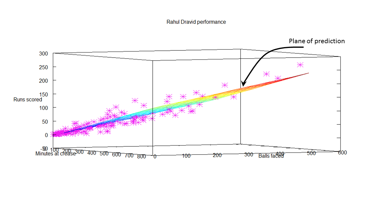
In my earlier post I was able to fit a ‘prediction plane’ based on the minutes at crease, balls faced versus the runs scored. But in this case a plane did not make sense as the wickets can only range from 0 – 10 and in most cases averaging between 3 and 5. So I plot the best fitting 3-D surface over the predicted hypothesis function. The steps performed are
1) The data for the different bowlers were cleaned with data which indicated (DNB – Did not bowl)
2) The Economy Rate (E) = Runs given/Overs and Strike Rate(SR) = Wickets/overs were calculated.
3) The product of Overs (O), and Economy(E) were stored as Over_Economy(OE)
4) The hypothesis function was computed as h(O, E, OE) = y
5) Theta was calculated using the Normal Equation. The Surface of Bowling Effectiveness( SBE) was then plotted. The plots for each of the bowler is shown below
Here are the plots
A) Anil Kumble
The data of Kumble, based on Overs bowled & Economy rate versus the Strike Rate is plotted as a 3-D scatter plot (pink crosses). The best fit as determined by solving the optimum theta using the Normal Equation is plotted as 3-D surface shown below.

The 3-D surface is what I have termed as ‘Surface of Bowling Effectiveness (SBE)’ as it depicts bowlers overall effectiveness as it plots the overs (O), ‘economy rate’ E against predicted ‘strike rate’ SR.
Here is another view

The theta values obtained for Kumble are
Theta =
0.104208
-0.043769
-0.016305
0.011949
And the cost at this theta is
Cost Function J = 0.0046269
B) B S Chandrasekhar
Here are the best optimal surface plot for Chandra with the data on O,E vs SR plotted as a 3D scatter plot. Note: The dataset for Chandrasekhar is smaller compared to the other two.
 Another view for Chandra

Theta values for B S Chandrasekhar are
Theta =
0.095780
-0.025377
-0.024847
0.023415
and the cost is
Cost Function J = 0.0032980
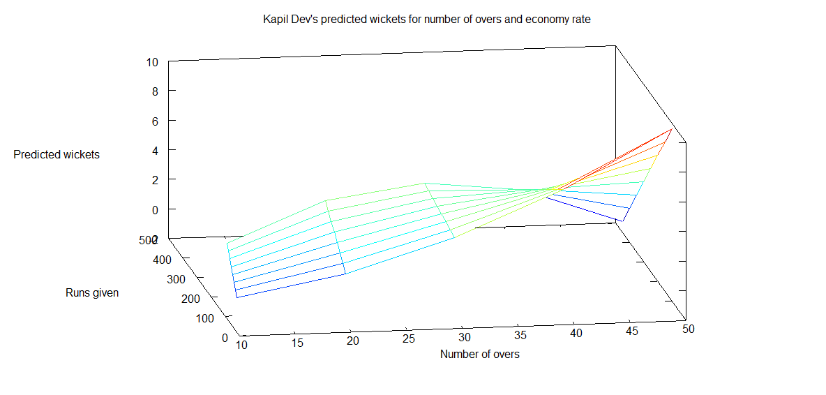
c) Kapil Dev
The plots for Kapil
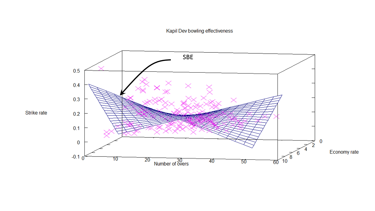
Another view of SBE for Kapil

The Theta values and cost function for Kapil are
Theta =
0.090219
0.027725
0.023894
-0.021434
Cost Function J = 0.0035123
2. Predicting wickets
In the previous section the optimum theta with the lowest Cost Function J was calculated. Based on the value of theta, the wickets that will be taken by a bowler can be computed as the product of the hypothesis function and theta. i.e.
y= h(x) * theta => Strike Rate (SR) = [1 O E OE] * theta
Now predicted wickets can be calculated as
wickets = Strike rate(SR) * Overs(O)
This is done for Kumble, Chandra and Kapil for different combinations of Overs(O) and Economy(E) rate.
Here are the results
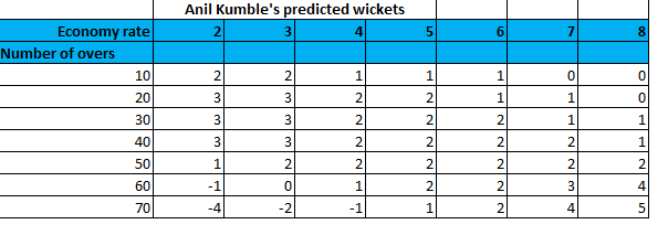
Predicted wickets for Anil Kumble
The plot of predicted wickets for Kumble is represented below
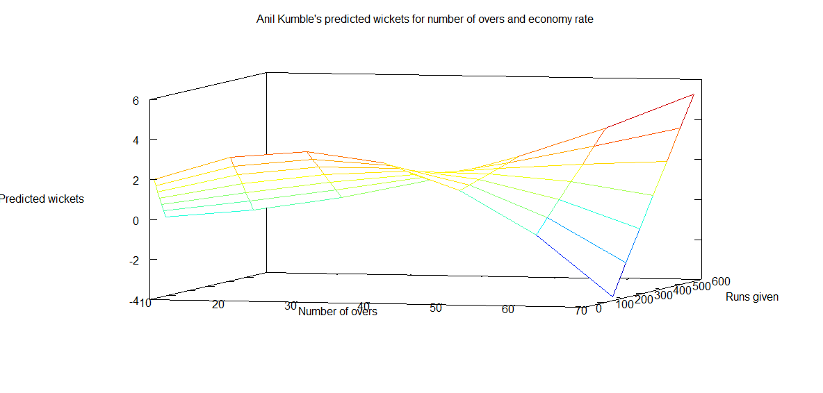
This can also be represented as a a table
Predicted wickets for B S Chandrasekhar
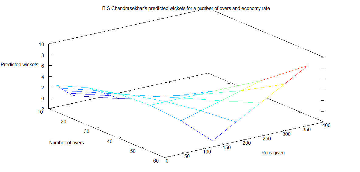
The table for Chandra

Predicted wickets for Kapil Dev
The plot
The predicted table from the hypothesis function for Kapil Dev

Observation: A closer look at the predicted wickets for Kapil, Kumble and B S Chandra shows an interesting aspect. The predicted number of wickets is higher for lower economy rates. With a little thought we can see bowlers on turning or pitches with a lot of movement can not only be more economical but can also be destructive and take a lot of wickets. Hence the higher wickets for lower economy rates!
Implementation details
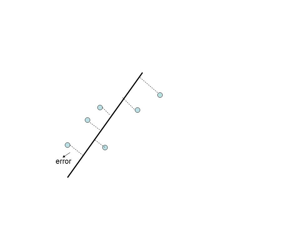
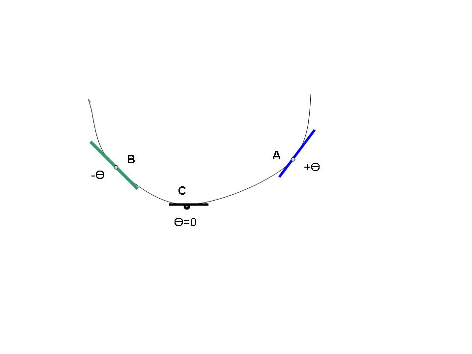
In this post I have used the Normal Equation to get the optimal values of theta for local minimum of the Gradient function. As mentioned above when I had run the 3D scatter plot fitting a 2D plane did not seem quite right. So I had to experiment with different polynomial equations first trying 2nd order, 3rd order and also the sqrt
I tried the following where ‘O is Overs, ‘E’ stands for Economy Rate and ‘SR’ the predicated Strike rate. Theta is the computed theta from the Normal Equation. The notation in Matrix notation is shown below
i) A linear plane
SR = [1 O E] * theta
ii) Using the sqrt function
SR = [1 sqrt(O) sqrt(E)] * theta
iii) Using 2nd order plynomial
SR = [1 O^2 E^2] * theta
iv) Using the 3rd order polynomial
SR = [1 O^3 E^3] * theta
v) Before finally settling on
SR = [1 O E OE] * theta
where OE = O .* E
The last one seemed to give me the lowest cost and also seemed the most logical visual choice.
A good resource to play around with different functions and check out the shapes of combinations of variables and polynomial order of equation is at WolframAlpha: Plotting and Graphics
Note 1: The gradient descent with the Normal Equation has been performed on the entire data set (approx 220 for Kumble & Kapil) and 99 for Chandra. The proper process for verifying a Machine Learning algorithm is to split the data set into (60% training data, 20% cross validation data and 20% as the test set). We need to validate the prediction function against the cross-validation set, fine tune it and finally ensure that it fits the test set samples well. However, this split was not done as the data set itself was very low. The entire data set was used to perform the optimal surface fit
Note 2: The optimal theta values have been chosen with a feature vector that is of the form
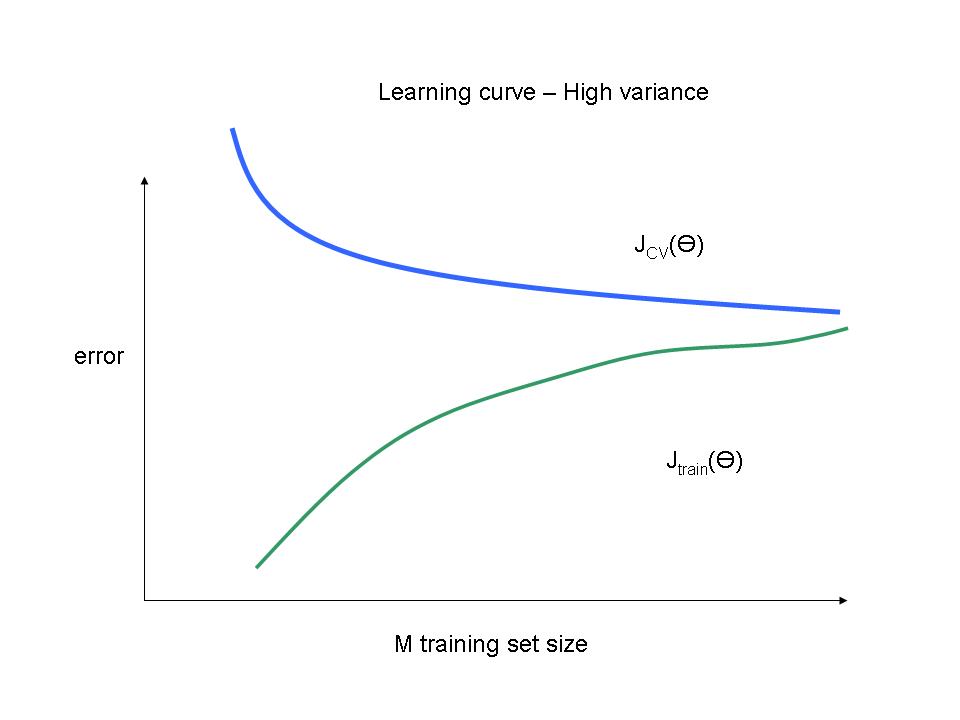
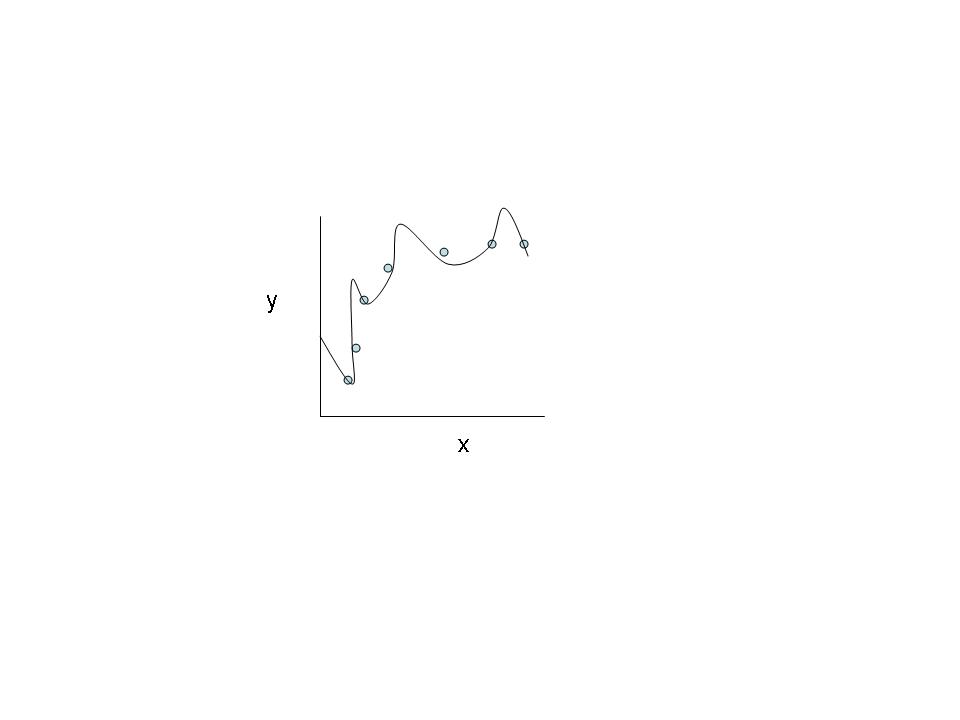
[1 x y x .* y] The Surface of Bowling Effectiveness’ has been plotted above. It may appear that there is a’high bias’ in the fit and an even better fit could be obtained by choosing higher order polynomials like
[1 x y x*y x^2 y^2 (x^2) .* y x .* (y^2)] or
[1 x y x*y x^2 y^2 x^3 y^3] etc
While we can get a better fit we could run into the problem of ‘high variance; and without the cross validation and test set we will not be able to verify the results, Hence the simpler option [1 x y x*y] was chosen
The Octave code outline and the data used can be cloned from GitHub at ml-bowling-analyze
Conclusion:
1) Predicted wickets: The predicted number of wickets is higher at lower economy rates
2) Comparing performances: There are different ways of looking at the results. One possible way is to check for a particular number of overs and economy rate who is most effective. Here is one way. Taking a small slice from each bowler’s predicted wickets table for anm Economy Rate=4.0 the predicted wickets are

From the above it does appear that Kapil is definitely more effective than the other two. However one could slice and dice in different ways, maybe the most economical for a given numbers and wickets combination or wickets taken in the least overs etc. Do add your thoughts. comments on my assessment or analysis
Also see
1. Analyzing cricket’s batting legends – Through the mirage with R
2. Masters of spin: Unraveling the web with R
You may also like
1. A peek into literacy in India:Statistical learning with R
2. A crime map of India in R: Crimes against women
3. What’s up Watson? Using IBM Watson’s QAAPI with Bluemix, NodeExpress – Part 1


 Checkout my book ‘Deep Learning from first principles Second Edition- In vectorized Python, R and Octave’. My book is available on Amazon as


