Thinking Web Scale (TWS-3): Map-Reduce – Bring compute to data

In the last decade and a half, there has arisen a class of problem that are becoming very critical in the computing domain. These problems deal with computing in a highly distributed environments. A key characteristic of this domain is the need to grow elastically with increasing workloads while tolerating failures without missing a beat. In short I would like to refer to this as ‘Web Scale Computing’ where the number of servers exceeds several 100’s and the data size is of the order of few hundred terabytes to several Exabytes.

There are several features that are unique to large scale distributed systems

The servers used are not specialized machines but regular commodity, off-the-shelf servers
Failures are not the exception but the norm. The design must be resilient to failures
There is no global clock. Each individual server has its own internal clock with its own skew and drift rates. Algorithms exist that can create a notion of a global clock
Operations happen at these machines concurrently. The order of the operations, things like causality and concurrency, can be evaluated through special algorithms like Lamport or Vector clocks
The distributed system must be able to handle failures where servers crash, disk fails or there is a network problem. For this reason data is replicated across servers, so that if one server fails the data can still be obtained from copies residing on other servers.
Since data is replicated there are associated issues of consistency. Algorithms exist that ensure that the replicated data is either ‘strongly’ consistent or ‘eventually’ consistent. Trade-offs are often considered when choosing one of the consistency mechanisms
Leaders are elected democratically. Then there are dictators who get elected through ‘bully’ing.

In some ways distributed systems behave like a murmuration of starlings (or a school of fish), where a leader is elected on the fly (pun unintended) and the starlings or fishes change direction based on a few (typically 6) closest neighbors.

This series of posts, Thinking Web Scale (TWS) , will be about Web Scale problems and the algorithms designed to address this. I would like to keep these posts more essay-like and less pedantic.

In the early days, computing used to be done in a single monolithic machines with its own CPU, RAM and a disk., This situation was fine for a long time, as technology promptly kept its date with Moore’s Law which stated that the “ computing power and memory capacity’ will double every 18 months. However this situation changed drastically as the data generated from machines grew exponentially – whether it was the call detail records, records from retail stores, click streams, tweets, and status updates of social networks of today

These massive amounts of data cannot be handled by a single machine. We need to ‘divide’ and ‘conquer this data for processing. Hence there is a need for a hundreds of servers each handling a slice of the data.

The first post is about the fairly recent computing paradigm “Map-Reduce”. Map- Reduce is a product of Google Research and was developed to solve their need to calculate create an Inverted Index of Web pages, to compute the Page Rank etc. The algorithm was initially described in a white paper published by Google on the Map-Reduce algorithm. The Page Rank algorithm now powers Google’s search which now almost indispensable in our daily lives.

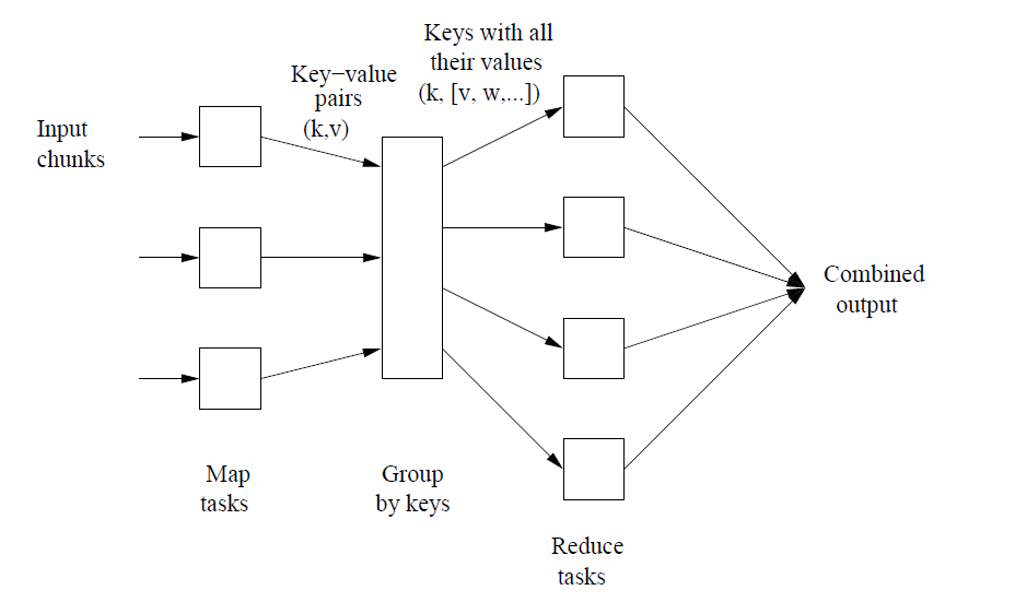
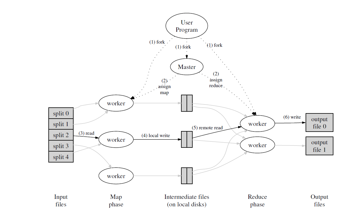
The Map-Reduce assumes that these servers are not perfect, failure-proof machines. Rather Map-Reduce folds into its design the assumption that the servers are regular, commodity servers performing a part of the task. The hundreds of terabytes of data is split into 16MB to 64MB chunks and distributed into a file system known as ‘Distributed File System (DFS)’. There are several implementations of the Distributed File System. Each chunk is replicated across servers. One of the servers is designated as the “Master’. This “Master’ allocates tasks to ‘worker’ nodes. A Master Node also keeps track of the location of the chunks and their replicas.

When the Map or Reduce has to process data, the process is started on the server in which the chunk of data resides.

The data is not transferred to the application from another server. The Compute is brought to the data and not the other way around. In other words the process is started on the server where the data, intermediate results reside

The reason for this is that it is more expensive to transmit data. Besides the latencies associated with data transfer can become significant with increasing distances

Map-Reduce had its genesis from a Lisp Construct of the same name

Where one could apply a common operation over a list of elements and then reduce the resulting list of elements with a reduce operation

The Map-Reduce was originally created by Google solve Page Rank problem Now Map-Reduce is used across a wide variety of problems.

The main components of Map-Reduce are the following

Mapper: Convert all d ∈ D to (key (d), value (d))
Shuffle: Moves all (k, v) and (k’, v’) with k = k’ to same machine.
Reducer: Transforms {(k, v1), (k, v2) . . .} to an output D’ k = f(v1, v2, . . .). …
Combiner: If one machine has multiple (k, v1), (k, v2) with same k then it can perform part of Reduce before Shuffle

A schematic of the Map-Reduce is included below\

Map Reduce is usually a perfect fit for problems that have an inherent property of parallelism. To these class of problems the map-reduce paradigm can be applied in simultaneously to a large sets of data. The “Hello World” equivalent of Map-Reduce is the Word count problem. Here we simultaneously count the occurrences of words in millions of documents

The map operation scans the documents in parallel and outputs a key-value pair. The key is the word and the value is the number of occurrences of the word. E.g. In this case ‘map’ will scan each word and emit the word and the value 1 for the key-value pair

So, if the document contained

“All men are equal. Some men are more equal than others”

Map would output

(all,1), (men,1), (are,1), (equal,1), (some,1), (men,1), (are,1), (equal,1), (than,1), (others,1)

The Reduce phase will take the above output and give sum all key value pairs with the same key

(all,1), (men,2), (are,2),(equal,2), (than,1), (others,1)

So we get to count all the words in the document

In the Map-Reduce the Master node assigns tasks to Worker nodes which process the data on the individual chunks

Map-Reduce also makes short work of dealing with large matrices and can crunch matrix operations like matrix addition, subtraction, multiplication etc.

Matrix-Vector multiplication

As an example if we consider a Matrix-Vector multiplication (taken from the book Mining Massive Data Sets by Jure Leskovec, Anand Rajaraman et al

For a n x n matrix if we have M with the value m_ij in the ith row and jth column. If we need to multiply this with a vector v_j,then the matrix-vector product of M x vj is given by x_i

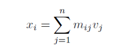
Here the product of m_ijx v_j can be performed by the map function and the summation can be performed by a reduce operation. The obvious question is, what if the vector vj or the matrix mij did not fit into memory. In such a situation the vector and matrix are divided into equal sized slices and performed acorss machines. The application would have to work on the data to consolidate the partial results.

Fortunately, several problems in Machine Learning, Computer Vision, Regression and Analytics which require large matrix operations. Map-Reduce can be used very effectively in matrix manipulation operations. Computation of Page Rank itself involves such matrix operations which was one of the triggers for the Map-Reduce paradigm.

Handling failures: As mentioned earlier the Map-Reduce implementation must be resilient to failures where failures are the norm and not the exception. To handle this the ‘master’ node periodically checks the health of the ‘worker’ nodes by pinging them. If the ping response does not arrive, the master marks the worker as ‘failed’ and restarts the task allocated to worker to generate the output on a server that is accessible.

Stragglers: Executing a job in parallel brings forth the famous saying ‘A chain is as strong as the weakest link’. So if there is one node which is straggler and is delayed in computation due to disk errors, the Master Node starts a backup worker and monitors the progress. When either the straggler or the backup complete, the master kills the other process.

Mining Social Networks, Sentiment Analysis of Twitterverse also utilize Map-Reduce.

However, Map-Reduce is not a panacea for all of the industry’s computing problems (see To Hadoop, or not to Hadoop)

But the Map-Reduce is a very critical paradigm in the distributed computing domain as it is able to handle mountains of data, can handle multiple simultaneous failures, and is blazingly fast.

Also see
1. A crime map of India in R: Crimes against women
2. What’s up Watson? Using IBM Watson’s QAAPI with Bluemix, NodeExpress – Part 1
3. Bend it like Bluemix, MongoDB with autoscaling – Part 2
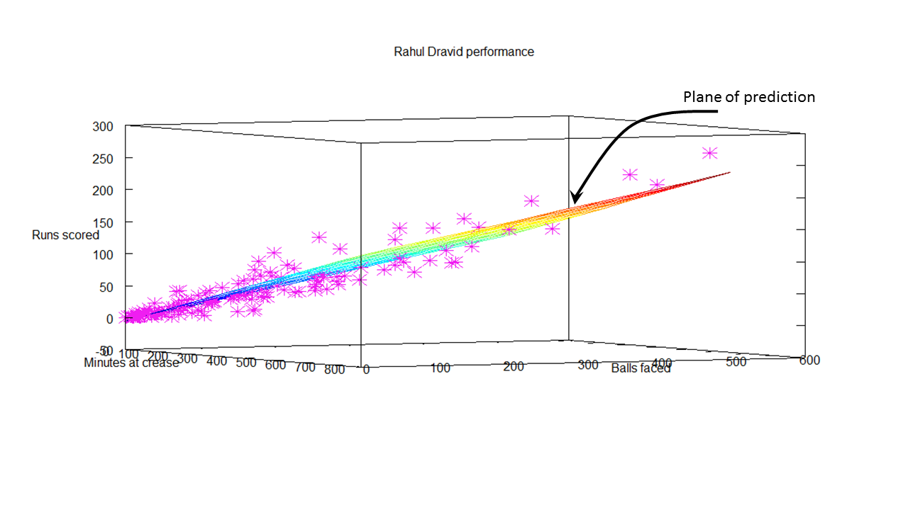
4. Informed choices through Machine Learning : Analyzing Kohli, Tendulkar and Dravid

To see all posts click ‘Index of Posts”

An Octave primer

Here is a simple Octave Primer. Octave is a powerful language for implementing Machine Learning algorithms. As I have mentioned its strength is its simplicity. I am including some basic commands with which you can get by implementing fairly complex code

%%Matrix
A matrix can be created as a = [1 2 3; 4 7 8; 12 35 14]; % This is 3 x 3 matrix
Matrix multiplication can be done between m x n * n x k matrix as follows

a = [4 56 3; 2 3 4]; b = [23 1; 3 12; 34 12]; % a = 3 x 2 matrix b = 2 x 3 matrix c = a*b; %% c = 3 x 2 * 2 * 3 = 3 x 3 matrix

c = 362 712 191 86

%%Inverse of a matrix can be obtained by
d = pinv(c); octave-3.2.4.exe:37> d = pinv(c) d = -8.2014e-004 6.7900e-003 1.8215e-003 -3.4522e-003

%%Transpose of a matrix
e = c'; % e is the transpose of done

octave-3.2.4.exe:38> e = c' e = 362 191 712 86

The following operations are done on all elements of a matrix or a vector
k = 5; a = [1 2; 3 4; 5 6]; k = 5.23; c = k * a; d = a - 2 e = a / 5 f = a .* a % Dot product g = a .^2; % Square each elements

%% Select slice of matrix
b = a(:,2); % Select column 2 of matrix a (all rows) c = a(2,:) % Select row of matrix 'a' (all columns)

d = [7 8; 8 9; 10 11; 12 13]; % 4 rows 2 columns d(2:3,:); %Select from rows 2 to 3 (all columns)

octave-3.2.4.exe:41> d d = 7 8 8 9 10 11 12 13 octave-3.2.4.exe:43> d(2:3,:) ans = 8 9 10 11

%% Appending rows to matrix
a = [ 4 5; 5 6; 5 7; 9 8]; % 4 x 2 b = [ 1 3; 2 4]; % 2 x 2 c = [ a; b] % stack a over b d = [b ; a] % stack b over a*b
octave-3.2.4.exe:44> a = [ 4 5; 5 6; 5 7; 9 8] % 4 x 2 a = 4 5 5 6 5 7 9 8

octave-3.2.4.exe:45>b = [ 1 3; 2 4] % 2 x 2 b = 1 3 2 4

octave-3.2.4.exe:46> c = [ a; b] % stack a over b c = 4 5 5 6 5 7 9 8 1 3 2 4

octave-3.2.4.exe:47> d = [b ; a] % stack b over a*b d = 1 3 2 4 4 5 5 6 5 7 9 8

%% Appending columns
a = [ 1 2 3; 3 4 5]; b = [ 1 2; 3 4]; c = [a b]; d = [b a];

octave-3.2.4.exe:48> a = [ 1 2 3; 3 4 5] a = 1 2 3 3 4 5

octave-3.2.4.exe:49>b = [ 1 2; 3 4] b = 1 2 3 4

octave-3.2.4.exe:50> c = [a b] c = 1 2 3 1 2 3 4 5 3 4

octave-3.2.4.exe:51>d = [b a] d = 1 2 1 2 3 3 4 3 4 5 %%Size of a matrix [c d ] = size(a);
Creating a matrix of all zeros or ones
d = ones(3,2); e = zeros(4,3);
%Appending an intercept term to a matrix
a = [1 2 3; 4 5 6]; %2 x 3 b = ones(2,1); a = [b a];

%% Plotting
Creating 2 vectors
x = [1 3 4 5 6]; y = [5 6 7 8 9]; plot(x,y);
%%Create labels
xlabel("X values); ylabel("Y values); axis([1 10 4 10]); % Set the range of x and y title("Test plot);

%%Creating a 3D scatter plot
If we have 3 column csv file then we can load the data as follows
data = load('values.csv'); X = data(:, 1:2); y = data(:, 3); scatter3(X(:,1),X(:,2),y,[],[240 15 15],'x'); % X(:,1) - x axis X(:,2) - yaxis y[] - z axis

%% Drawing a 3D mesh
x = linspace(0,xrange + 20,10); y = linspace(1,yrange+ 20,10); [XX, YY ] = meshgrid(x,y);
[a b] = size(XX)

Draw the mesh
for i=1:a, for j= 1:b, ZZ(i,j) = [1 (XX(i,j)-mu(1))/sigma(1) (YY(i,j) - mu(2))/sigma(2) ] * theta; end; end; mesh(XX,YY,ZZ);

For more details please see post Informed choices using Machine Learning 2- Pitting Kumble, Kapil and B S Chandra

%% Creating different polynomial equations
Let X be a feature vector
then
X = [X X.^2 X^3] %X X^2 X^3

This can be created using a for loop as follows
for i= 1:n xtemp = xinput .^i; x = [x xtemp]; end;

Finally while doing multivariate regression if we wanted to create polynomial terms of higher we could do as follows. Let us say we have a feature vector X made of 3 features x1, x2,

Let us say we wanted to create a polynomial of the form x1^2 x1.x2 x2^2 then we could create X as

X = [X(:,1) .^2 X(:,1) . X(:,2) X(:,2) .^2]

As you can see Octave is really powerful language for Machine Learning and has just a few handful of constructs with which one can implement powerful Machine Learning algorithms

Applying the principles of Machine Learning

While working with multivariate regression there are certain essential principles that must be applied to ensure the correctness of the solution while being able to pick the most optimum solution. This is all the more important when the problem has a large number of features. In this post I apply these important principles to a regression data set which I was able to pull of the internet. This data set was taken from the UCI Machine Learning repository and deals with Boston housing data. The housing data provides the cost of house in Boston suburbs given the number of rooms, the connectivity to main highways, and crime rate in the area and several other data. There are a total of 506 data points in this data set with a total of 13 features.

This seemed a reasonable dataset to start to try out the principles of Machine Learning I had picked up from Coursera’s ML course.

Out of a total of 13 features 2 features ’ZN’ and ‘CHAS’ proximity to Charles river were dropped as the values were mostly zero in these columns . The remaining 11 features were used to map to the output variable of the price.

The following key rules have been applied on the

The dataset was divided into training samples (60%), cross-validation set (20%) and test set (20%) using a random index
Try out different polynomial functions while performing gradient descent to determine the theta values
Different combinations of ‘alpha’ learning rate and ‘lambda’ the regularization parameter were tried while performing gradient descent
The error rate is then calculated on the cross-validation and test set
The theta values that were obtained for the lowest cost for a polynomial was used to compute and plot the learning curve for the different polynomials against increasing number of training and cross-validation test samples to check for bias and variance.
The plot of the cost versus the polynomial degree was plotted to obtain the best fit polynomial for the data set.

A multivariate regression hypothesis can be represented as

hθ(x) = θ₀ + θ₁x₁ + θ₂x₂ + θ₃x₃ + θ₄x₄ + …
And the cost can is determined as
J(θ₀, θ₁, θ₂, θ₃..) = 1/2m ∑ (h_Θ (xⁱ) -yⁱ)²
The implementation was done using Octave. As in my previous posts some functions have not been include to comply with Coursera’s Honor Code. The code can be cloned from GitHub at machine-learning-principles

a) housing compute.m. In this module I perform gradient descent for different polynomial degrees and check the error that is obtained when using the computed theta on the cross validation and test set

max_degrees =4; J_history = zeros(max_degrees, 1); Jcv_history = zeros(max_degrees, 1); for degree = 1:max_degrees; [J Jcv alpha lambda] = train_samples(randidx, training,cross_validation,test_data,degree); end;

b) train_samples.m – This module uses gradient descent to check the best fit for a given polynomial degree for different combinations of alpha (learning rate) and lambda( regularization).

for i = 1:length(alpha_arr), for j = 1:length(lambda_arr) alpha = alpha_arr{i}; lambda= lambda_arr{j}; % Perform Gradient descent % Compute error for training sample for computed theta values % Compute the error rate for the cross validation samples % Compute the error rate against the test set end; end;

c) cross_validation.m – This module uses the theta values to compute cost for the cross validation set

d) test-samples.m – This modules computes the error when using the trained theta on the test set

e) poly.m – This module constructs polynomial vectors based on the degree as follows
function [x] = poly(xinput, n) x = []; for i= 1:n xtemp = xinput .^i; x = [x xtemp]; end;

e) learning_curve.m – The learning curve module plots the error rate for increasing number of training and cross validation samples. This is done as follows. For the theta with the lowest cost as determined by gradient descent
for i from 1 to 100

Compute the error for ‘i’ training samples
Compute the error for ‘i’ cross-validation
Plot the learning curve to determine the bias and variance of the polynomial fit

This is included below
for i = 1: 100 xsample = xtrain(1:i,:); ysample = ytrain(1:i,:); size(xsample); size(ysample); [xsample] = poly(xsample,degree); xsample= [ones(i, 1) xsample]; [c d] = size(xsample); theta = zeros(d, 1); % Minimize using fmincg J = computeCost(xsample, ysample, theta); Jtrain(i) = J; xsample_cv = xcv(1:i,:); ysample_cv = ycv(1:i,:); [xsample_cv] = poly(xsample_cv,degree); xsample_cv= [ones(i, 1) xsample_cv]; J_cv = computeCost(xsample_cv, ysample_cv,theta) Jcv(i) = J_cv; end;

Finally a plot is done been different lambda and the cost.

The results are included below

A) Polynomial degree 1
Convergence graph

Learning curve

The above figure does show a stronger bias. Note: the learning curve was done with around 100 samples
B) Polynomial degree 2

Convergence graph

Learning curve

The learning curve for degree 2 shows a stronger variance.

C) Polynomial degree 3
Convergence graph

Learning curve

D) Polynomial degree 4
Convergence graph

E) Learning curve

This plot is useful to determine which polynomial degree will give the best fit for the dataset and the lowest cost

Clearly from the above it can be seen that degree 2 will give a good fit for the data set.

F) Lambda vs Cost function

The above code demonstrates some key principles while performing multivariate regression
The code can be cloned from GitHub at machine-learning-principles

Informed choices through Machine Learning-2: Pitting together Kumble, Kapil, Chandra

Continuing my earlier ‘innings’, of test driving my knowledge in Machine Learning acquired via Coursera, I now turn my attention towards the bowling performances of our Indian bowling heroes. In this post I give a slightly different ‘spin’ to the bowling analysis and hope I can ‘swing’ your opinion based on my assessment.

I guess that is enough of my cricketing ‘double-speak’ for now and I will get down to the real business of my bowling analysis!

If you are passionate about cricket, and love analyzing cricket performances, then check out my 2 racy books on cricket! In my books, I perform detailed yet compact analysis of performances of both batsmen, bowlers besides evaluating team & match performances in Tests , ODIs, T20s & IPL. You can buy my books on cricket from Amazon at $12.99 for the paperback and $4.99/$6.99 respectively for the kindle versions. The books can be accessed at Cricket analytics with cricketr and Beaten by sheer pace-Cricket analytics with yorkr A must read for any cricket lover! Check it out!!

As in my earlier post Informed choices through Machine Learning – Analyzing Kohli, Tendulkar and Dravid ,the first part of the post has my analyses and the latter part has the details of the implementation of the algorithm. Feel free to read the first part and either scan or skip the latter.

To perform this analysis I have skipped the data on our recent crop of new bowlers. The reason being that data is scant on these bowlers, besides they also seem to have a relatively shorter shelf life (hope there are a couple of finds in this Australian tour of Dec 2014). For the analyses I have chosen B S Chandrasekhar, Kapil Dev Anil Kumble. My rationale as to why I chose the above 3

B S Chandrasekhar also known as “Chandra’ was one of the most lethal leg spinners in the late 1970’s. He had a very dangerous combination of fast leg breaks, searing tops spins interspersed with the occasional googly. On many occasions he would leave most batsmen completely clueless.

Kapil Nikhanj Dev, the Haryana Hurricane who could outwit the most technically sound batsmen through some really clever bowling. His variations were almost always effective and he would achieve the vital breakthrough outsmarting the opponent.

And finally Anil Kumble, I chose Kumble because in my opinion he is truly the embodiment of the ‘thinking’ bowler. Many times I have seen Kumble repeatedly beat batsmen. It was like he was telling the batsman ‘check’ as he bowled faster leg breaks, flippers, a straighter delivery or top spins before finally crashing into the wickets or trapping the batsmen. It felt he was saying ‘checkmate dude!’

I have taken the data for the 3 bowlers from ESPN Cricinfo. Only the Test matches were considered for the analyses. All tests against all oppositions both at home and away were included

The assumptions taken and basis of the computation is included below
a.The data is based on the following 2 input variables a) Overs bowled b) Runs given. The output variable is ‘Wickets taken’

b.To my surprise I found that in the late 1970’s when BS Chandrasekhar used to bowl, an over had 8 balls for matches in Australia. So, I had to normalize this data for Chandra to make it on par with the others. Hence for Chandra where the overs were made up of 8 balls the overs was calculated as follows
Overs (O) = (Overs * 8)/6

c.The Economy rate E was calculated as below
E = Overs/runs was chosen as input variable to take into account fewer runs given by the bowler

d.The output variable was re-calculated as Strike Rate (SR) to determine the ‘bowling effectiveness’
Strike Rate = Wickets/Overs
(not be confused with a batsman’s strike rate batsman strike rate = runs/ balls faced)

e.Hence the analysis is based on
f(O,E) = SR
An outline of the Octave code and the data used can be cloned from GitHub at ml-bowling-analyze

1. Surface of Bowling Effectiveness (SBE)
In my earlier post I was able to fit a ‘prediction plane’ based on the minutes at crease, balls faced versus the runs scored. But in this case a plane did not make sense as the wickets can only range from 0 – 10 and in most cases averaging between 3 and 5. So I plot the best fitting 3-D surface over the predicted hypothesis function. The steps performed are

1) The data for the different bowlers were cleaned with data which indicated (DNB – Did not bowl)
2) The Economy Rate (E) = Runs given/Overs and Strike Rate(SR) = Wickets/overs were calculated.
3) The product of Overs (O), and Economy(E) were stored as Over_Economy(OE)
4) The hypothesis function was computed as h(O, E, OE) = y
5) Theta was calculated using the Normal Equation. The Surface of Bowling Effectiveness( SBE) was then plotted. The plots for each of the bowler is shown below

Here are the plots

A) Anil Kumble
The data of Kumble, based on Overs bowled & Economy rate versus the Strike Rate is plotted as a 3-D scatter plot (pink crosses). The best fit as determined by solving the optimum theta using the Normal Equation is plotted as 3-D surface shown below.

The 3-D surface is what I have termed as ‘Surface of Bowling Effectiveness (SBE)’ as it depicts bowlers overall effectiveness as it plots the overs (O), ‘economy rate’ E against predicted ‘strike rate’ SR.
Here is another view

The theta values obtained for Kumble are
Theta =
0.104208
-0.043769
-0.016305
0.011949

And the cost at this theta is
Cost Function J = 0.0046269

B) B S Chandrasekhar
Here are the best optimal surface plot for Chandra with the data on O,E vs SR plotted as a 3D scatter plot. Note: The dataset for Chandrasekhar is smaller compared to the other two.
Another view for Chandra

Theta values for B S Chandrasekhar are
Theta =
0.095780
-0.025377
-0.024847
0.023415
and the cost is
Cost Function J = 0.0032980

c) Kapil Dev
The plots for Kapil

Another view of SBE for Kapil

The Theta values and cost function for Kapil are
Theta =
0.090219
0.027725
0.023894
-0.021434
Cost Function J = 0.0035123

2. Predicting wickets
In the previous section the optimum theta with the lowest Cost Function J was calculated. Based on the value of theta, the wickets that will be taken by a bowler can be computed as the product of the hypothesis function and theta. i.e.

y= h(x) * theta => Strike Rate (SR) = [1 O E OE] * theta
Now predicted wickets can be calculated as

wickets = Strike rate(SR) * Overs(O)
This is done for Kumble, Chandra and Kapil for different combinations of Overs(O) and Economy(E) rate.

Here are the results
Predicted wickets for Anil Kumble
The plot of predicted wickets for Kumble is represented below

This can also be represented as a a table

Predicted wickets for B S Chandrasekhar

The table for Chandra

Predicted wickets for Kapil Dev

The plot

The predicted table from the hypothesis function for Kapil Dev

Observation: A closer look at the predicted wickets for Kapil, Kumble and B S Chandra shows an interesting aspect. The predicted number of wickets is higher for lower economy rates. With a little thought we can see bowlers on turning or pitches with a lot of movement can not only be more economical but can also be destructive and take a lot of wickets. Hence the higher wickets for lower economy rates!

Implementation details
In this post I have used the Normal Equation to get the optimal values of theta for local minimum of the Gradient function. As mentioned above when I had run the 3D scatter plot fitting a 2D plane did not seem quite right. So I had to experiment with different polynomial equations first trying 2^nd order, 3^rd order and also the sqrt

I tried the following where ‘O is Overs, ‘E’ stands for Economy Rate and ‘SR’ the predicated Strike rate. Theta is the computed theta from the Normal Equation. The notation in Matrix notation is shown below

i) A linear plane
SR = [1 O E] * theta

ii) Using the sqrt function
SR = [1 sqrt(O) sqrt(E)] * theta

iii) Using 2^nd order plynomial
SR = [1 O^2 E^2] * theta

iv) Using the 3^rd order polynomial
SR = [1 O^3 E^3] * theta

v) Before finally settling on
SR = [1 O E OE] * theta

where OE = O .* E

The last one seemed to give me the lowest cost and also seemed the most logical visual choice.

A good resource to play around with different functions and check out the shapes of combinations of variables and polynomial order of equation is at WolframAlpha: Plotting and Graphics

Note 1: The gradient descent with the Normal Equation has been performed on the entire data set (approx 220 for Kumble & Kapil) and 99 for Chandra. The proper process for verifying a Machine Learning algorithm is to split the data set into (60% training data, 20% cross validation data and 20% as the test set). We need to validate the prediction function against the cross-validation set, fine tune it and finally ensure that it fits the test set samples well. However, this split was not done as the data set itself was very low. The entire data set was used to perform the optimal surface fit

Note 2: The optimal theta values have been chosen with a feature vector that is of the form
[1 x y x .* y] The Surface of Bowling Effectiveness’ has been plotted above. It may appear that there is a’high bias’ in the fit and an even better fit could be obtained by choosing higher order polynomials like
[1 x y x*y x^2 y^2 (x^2) .* y x .* (y^2)] or
[1 x y x*y x^2 y^2 x^3 y^3] etc
While we can get a better fit we could run into the problem of ‘high variance; and without the cross validation and test set we will not be able to verify the results, Hence the simpler option [1 x y x*y] was chosen

The Octave code outline and the data used can be cloned from GitHub at ml-bowling-analyze

Conclusion:

1) Predicted wickets: The predicted number of wickets is higher at lower economy rates
2) Comparing performances: There are different ways of looking at the results. One possible way is to check for a particular number of overs and economy rate who is most effective. Here is one way. Taking a small slice from each bowler’s predicted wickets table for anm Economy Rate=4.0 the predicted wickets are

From the above it does appear that Kapil is definitely more effective than the other two. However one could slice and dice in different ways, maybe the most economical for a given numbers and wickets combination or wickets taken in the least overs etc. Do add your thoughts. comments on my assessment or analysis

Also see
1. Analyzing cricket’s batting legends – Through the mirage with R
2. Masters of spin: Unraveling the web with R

Informed choices through Machine Learning – Analyzing Kohli, Tendulkar and Dravid

Having just completed the highly stimulating & inspiring Stanford’s Machine Learning course at Coursera, by the incomparable Professor Andrew Ng I wanted to give my newly acquired knowledge a try. As a start, I decided to try my hand at analyzing one of India’s fastest growing stars, namely Virat Kohli . For the data on Virat Kohli I used the ‘Statistics database’ at ESPN Cricinfo. To make matters more interesting, I also pulled data on the iconic Sachin Tendulkar and the Mr. Dependable, Rahul Dravid.

(Also do check out my R package cricketr Introducing cricketr! : An R package to analyze performances of cricketers and my interactive Shiny app implementation using my R package cricketr – Sixer – R package cricketr’s new Shiny avatar )

Based on the data of these batsmen I perform some predictions with the help of machine learning algorithms. That I have a proclivity for prediction, is not surprising, considering the fact that my Dad was an astrologer who had reasonable success at this esoteric art. While he would be concerned with planetary positions, about Rahu in the 7th house being in the malefic etc., I on the other hand focus my predictions on multivariate regression analysis and K-Means. The first part of my post gives the results of my analysis and some predictions for Kohli, Tendulkar and Dravid.

The second part of the post contains a brief outline of the implementation and not the actual details of implementation. This is ensure that I don’t violate Coursera’s Machine Learning’ Honor Code.

This code, data used and the output obtained can be accessed at GitHub at ml-cricket-analysis

Analysis and prediction of Kohli, Tendulkar and Dravid with Machine Learning As mentioned above, I pulled the data for the 3 cricketers Virat Kohli, Sachin Tendulkar and Rahul Dravid. The data taken from Cricinfo database for the 3 batsman is based on the following assumptions

Only ‘Minutes at Crease’ and ‘Balls Faced’ were taken as features against the output variable ‘Runs scored’
Only test matches were taken. This included both test ‘at home’ and ‘away tests’
The data was cleaned to remove any DNB (did not bat) values
No extra weightage was given to ‘not out’. So if Kohli made ‘28*’ 28 not out, this was taken to be 28 runs

Regression Analysis for Virat Kohli There are 51 data points for Virat Kohli regarding Tests played. The data for Kohli is displayed as a 3D scatter plot where x-axis is ‘minutes’ and y-axis is ‘balls faced’. The vertical z-axis is the ‘runs scored’. Multivariate regression analysis was performed to find the best fitting plane for the runs scored based on the selected features of ‘minutes’ and ‘balls faced’.

This is based on minimizing the cost function and then performing gradient descent for 400 iterations to check for convergence. This plane is shown as the 3-D plane that provides the best fit for the data points for Kohli. The diagram below shows the prediction plane of expected runs for a combination of ‘minutes at crease’ and ‘balls faced’. Here are 2 such plots for Virat Kohli. Another view of the prediction plane Prediction for Kohli I have also computed the predicted runs that will be scored by Kohli for different combinations of ‘minutes at crease’ and ‘balls faced’. As an example, from the table below, we can see that the predicted runs for Kohli after being in the crease for 110 minutes and facing 135 balls is 54 runs. Regression analysis for Sachin Tendulkar There was a lot more data on Tendulkar and I was able to dump close to 329 data points. As before the ‘minutes at crease’, ‘balls faced’ vs ‘runs scored’ were plotted as a 3D scatter plot. The prediction plane is calculated using gradient descent and is shown as a plane in the diagram below Another view of this below Predicted runs for Tendulkar The table below gives the predicted runs for Tendulkar for a combination of time at crease and balls faced. Hence, Tendulkar will score 57 runs in 110 minutes after facing 135 deliveries Regression Analysis for Rahul Dravid The same was done for ‘the Wall’ Dravid. The prediction plane is below Predicted runs for Dravid The predicted runs for Dravid for combinations of batting time and balls faced is included below. The predicted runs for Dravid after facing 135 deliveries in 110 minutes is 44. Further analysis While the ‘prediction plane’ was useful, it somehow does not give a clear picture of how effective each batsman is. Clearly the 3D plots show at least 3 clusters for each batsman. For all batsmen, the clustering is densest near the origin, become less dense towards the middle and sparse on the other end. This is an indication during which session during their innings the batsman is most prone to get out. So I decided to perform K-Means clustering on the data for the 3 batsman. This gives the 3 general tendencies for each batsman. The output is included below

K-Means for Virat The K-Means for Virat Kohli indicate the follow

Centroids found 255.000000 104.478261 19.900000
Centroids found 194.000000 80.000000 15.650000
Centroids found 103.000000 38.739130 7.000000

Analysis of Virat Kohli’s batting tendency
Kohli has a 45.098 percent tendency to bat for 104 minutes, face 80 balls and score 38 runs
Kohli has a 39.216 percent tendency to bat for 19 minutes, face 15 balls and score 7 runs
Kohli has a 15.686 percent tendency to bat for 255 minutes, face 194 balls and score 103 runs

The computation of this included in the diagram below

K-means for Sachin Tendulkar

The K-Means for Sachin Tendulkar indicate the following

Centroids found 166.132530 353.092593 43.748691
Centroids found 121.421687 250.666667 30.486911
Centroids found 65.180723 138.740741 15.748691

Analysis of Sachin Tendulkar’s performance

Tendulkar has a 58.232 percent tendency to bat for 43 minutes, face 30 balls and score 15 runs
Tendulkar has a 25.305 percent tendency to bat for 166 minutes, face 121 balls and score 65 runs
Tendulkar has a 16.463 percent tendency to bat for 353 minutes, face 250 balls and score 138 runs
K-Means for Rahul Dravid

Centroids found 191.836364 409.000000 50.506024
Centroids found 137.381818 290.692308 34.493976
Centroids found 56.945455 131.500000 13.445783

Analysis of Rahul Dravid’s performance
Dravid has a 50.610 percent tendency to bat for 50 minutes, face 34 balls and score 13 runs
Dravid has a 33.537 percent tendency to bat for 191 minutes, face 137 balls and score 56 runs
Dravid has a 15.854 percent tendency to bat for 409 minutes, face 290 balls and score 131 runs
Some implementation details The entire analysis and coding was done with Octave 3.2.4. I have included the outline of the code for performing the multivariate regression. In essence the pseudo code for this

Read the batsman data (Minutes, balls faced versus Runs scored)
Calculate the cost
Perform Gradient descent

The cost was plotted against the number of iterations to ensure convergence while performing gradient descent Plot the 3-D plane that best fits the data
The outline of this code, data used and the output obtained can be accessed at GitHub at ml-cricket-analysis

Conclusion: Comparing the results from the K-Means Tendulkar has around 48% to make a score greater than 60
Tendulkar has a 25.305 percent tendency to bat for 166 minutes, face 121 balls and score 65 runs
Tendulkar has a 16.463 percent tendency to bat for 353 minutes, face 250 balls and score 138 runs

And Dravid has a similar 48% tendency to score greater than 56 runs
Dravid has a 33.537 percent tendency to bat for 191 minutes, face 137 balls and score 56 runs
Dravid has a 15.854 percent tendency to bat for 409 minutes, face 290 balls and score 131 runs

Kohli has around 45% to score greater than 38 runs
Kohli has a 45.098 percent tendency to bat for 104 minutes, face 80 balls and score 38 runs

Also Kohli has a lesser percentage to score lower runs as against the other two
Kohli has a 39.216 percent tendency to bat for 19 minutes, face 15 balls and score 7 runs

The results must be looked in proper perspective as Kohli is just starting his career while the other 2 are veterans. Kohli has a long way to go and I am certain that he will blaze a trail of glory in the years to come!

Watch this space!

Also see
1. My book ‘Practical Machine Learning with R and Python’ on Amazon
2.Introducing cricketr! : An R package to analyze performances of cricketers
3.Informed choices with Machine Learning 2 – Pitting together Kumble, Kapil and Chandra
4. Analyzing cricket’s batting legends – Through the mirage with R
5. What’s up Watson? Using IBM Watson’s QAAPI with Bluemix, NodeExpress – Part 1
6. Bend it like Bluemix, MongoDB with autoscaling – Part 1

The language R

In the universe of programming languages there is a rising staR. It is moving fasteR and getting biggeR and brighteR!

Ok, you get the hint! It is the language R or the R Language.

R language is the successor to the language S. R is extremely powerful for statistical computing and processing. It is an interpreted language much like Python, Perl. The power of the language R comes from the 4000+ software packages that make the R language almost indispensable for any type of statistical computing.

As I mentioned above in my opinion, R, is soon going to play a central role in the technological world. In today’s world we are flooded with data from all sides. To make sense of this information overload we need techniques like Big Data, Analytics and machine learning to make sense of this data deluge. This is where R with its numerous packages that make short work of data becomes critical. The packages also have very interesting graphic packages to display the data in many forms for faster analysis and easier consumption.

The language R can easily ingest large sets of data in CSV format and perform many computations on them. R language is being used in machine learning, data mining, classification and clustering, text mining besides also being utilized in sentiment analysis from social networks.

The R language contains the usual programming constructs namely logical, loops, assignment etc. The language enables to easily assign values to vectors, matrices, arrays and perform all the associated operations on them.

The R Language can be installed from R-project. The R Language package comes with many datasets which are data collected from various sources. One such dataset is the Iris dataset. The Iris dataset is dataset about the Iris plant( Iris is a genus of 260–300[1][2] species of flowering plants with showy flowers).

The dataset contains 5 parameters

1) Sepal length 2) Sepal Width 3) Petal length 4) Petal width 5) Species

This dataset has been used in many research papers. R allows you to easily perform any sophisticated set of statistical operations on this data set. Included below are a sample set of operations you can perform on the Iris dataset or any dataset

> iris[1:5,]

Sepal.Length Sepal.Width Petal.Length Petal.Width Species

1 5.1 3.5 1.4 0.2 setosa

2 4.9 3.0 1.4 0.2 setosa

3 4.7 3.2 1.3 0.2 setosa

4 4.6 3.1 1.5 0.2 setosa

5 5.0 3.6 1.4 0.2 setosa

> summary(iris)

Sepal.Length Sepal.Width Petal.Length Petal.Width Species

Min. :4.300 Min. :2.000 Min. :1.000 Min. :0.100 setosa :50

1st Qu.:5.100 1st Qu.:2.800 1st Qu.:1.600 1st Qu.:0.300 versicolor:50

Median :5.800 Median :3.000 Median :4.350 Median :1.300 virginica :50

Mean :5.843 Mean :3.057 Mean :3.758 Mean :1.199

3rd Qu.:6.400 3rd Qu.:3.300 3rd Qu.:5.100 3rd Qu.:1.800

Max. :7.900 Max. :4.400 Max. :6.900 Max. :2.500

>hist(iris$Sepal.Length)

Here is a scatter plot of the Petal width, sepal length and sepal width

>scatterplot3d(iris$Petal.Width, iris$Sepal.Length, iris$Sepal.Width)

As can be seen R can really make short work of data with the numerous packages that come along with it. I have just skimmed the surface of R language.

I hope this has whetted your appetite. Do give R a spin!

Watch this space!

Also see
1. Designing a Social Web Portal
2. Design principles of scalable, distributed systems
3. A Cloud Medley with IBM’s Bluemix, Cloudant and Node.js
4. Programming Zen and now – Some essential tips -2
5. Fun simulation of a Chain in Android

Find me on Google+

Simplifying ML: Recommender Systems – Part 7

In this age of Amazon, Netflix and App stores where products, movies and apps are purchased online the method of up-selling and cross-selling online is through the use of recommender based systems.

When you go to site like Amazon/Flipkart or purchase apps on App store/Google Play we often see things like “People who bought this book/app also bought X, Y, Z”. These recommendations are the recommender system algorithms in action.

Recently, Netflix ran a competition in which users had to come with the best algorithm to recommend films that a user would also like. The prize money for this was of the order of $1 million. That’s how critical recommender systems are to organizations of today where most of the transactions happen on the web.

Typically users are asked to give a rating of 1 to 5 with 1 being the lowest and 5 being the highest. So for example if we had classics like Moby Dick, Great Expectations and current best sellers like The Client, The da Vinci Code and a Science Fiction like 2001- A Space Odyssey we can expect that different people will rate the books differently. Obviously not everybody would have read every book in the list and some elements would be blank.

Recommender Systems are based on machine learning algorithms. The goal of these algorithms is to predict what score any user would give to books they did not rate. In other words what would be rating the buyers would give for books or apps they did not buy. So if the algorithm predicts a high rating then we could recommend that the user would also ‘like’ them. Or we could give recommendations of books/apps bought by users who bought the books/apps bought by this user.

The notation is

n_u = Number of users

n_b= Number of books

r^(i,j) = Boolean whether user j rated a book i

y^(i,j) = The rating user j gave book i

m_j = The number of books that user j rated

Content based recommendation

In a typical content based recommendation algorithm we assume that we have data about some items we want to recommend rating for e.g. books/products/apps. In the example for books bought in an online bookstore we assume some features in our case ‘classic’, “fiction” etc

So each book has its own feature vector where x¹is the feature vector of the first book x² feature vector of the 2nd book and so on

This can be done through linear regression by minimizing the cost function of the sum of squared errors from the predicted value

So for a parameter vector Ɵ^jand a feature vector xⁱ the recommender system will try to predict the rating that a user j will give a book i.

This can be written as

Number of stars (rating) = (θ^j)^T xⁱ

This reduces to the minimization problem over all θ^j for r=1

min 1/2m Σ ((θj)^T xⁱ – y ^i,j)²

θ^ji:r=1

Adding the regularization term this becomes

min 1/2m Σ((θ^j)^T xⁱ – y ^i,j)² + λ/2m(Σ θ^j)²

θ^ji:r=1

The recommender algorithm in essence tries to learn parameters θ^j for a set of features of xⁱthe chosen system for e.g. books in this case.

The recommender tries to learn the parameters for all the users

min 1/2m Σ Σ((θ^j)^T xⁱ – y ^i,j)² + λ/2m(Σ Σ θ^j)²

θ¹…θⁿi:r=1

The minimization is performed by gradient descent as

Θ^j_k:= Θ^j_k – α (Σ((θ^j)^T xⁱ – y ^i,j)xⁱ + λ Θ^j_k

Recommender systems tries to learn the parameters for a set of chosen features over all users. Based on the learnt paramaters it then tries to predict the rating the user would give to books/apps that he is yet to purchase and push up those apps for which the user is likely to give a high rating based on the given set of ratings.

Recommender systems contribute substantially to the revenues of e-commerce sites like Amazon, Flipkart, Netflix etc

Note: This post, line previous posts on Machine Learning, is based on the Coursera course on Machine Learning by Professor Andrew Ng

Find me on Google+

Perils and pitfalls of Big Data

Big Data is hurtling towards us in a big way. It is already in the news and the blip seems to getting bigger. Big Data will soon become the key driver for almost any kind of decision that is to be made in manufacturing, retail, finance all the way to astronomy, oceanography etc. The common aspect of all industries and areas is that data is generated in the order of several petabytes to exabytes. Big Data is the technique to analyze such large volumes of data.

Big Data represents the technique to handle the huge deluge of data that is already becoming enmeshed in our lives. Multiple disparate, varied streams of data (text. tweets, click streams, html) flow through with tremendous volume & velocity. The key aspects of data in the world are the volume, variety and the velocity. It is never ending and never seems to stop. How do we handle this deluge? How do we make sense of this data is what Big Data is all about.

Big Data provides algorithms to find patterns, determine trends or classify data depending on the features provided. It is supposed to enable the decision makes to make key decisions based on the answers the algorithms spew forth.

Big Data is also complicated by the fact that data comes is multiple forms from click streams, tweets, html, texts, CSVs, structured and non –structured data.

The ability to detect patterns, determine trends, classify, identify outliers is no easy task

In this post I try to take a philosophical look at Big Data and ask whether it can really help us. Will it help or will take is on wild goose chase? Can we trust the results?

Big Data depends on algorithms to make sense of data. Big Data deals with data that is in the order of Petabytes to Exabytes. At this scale with multiple features our cognitive abilities are of no use. We must rely on machines and algorithms to make sense of these large amounts of data. Our mind can handle a few hundred data points and at most 3 dimensions. Beyond that the data can hardly make any sense.

Data by itself, in the absence of features & algorithms, is indistinguishable from noise. It is data science that makes sense of data. Data science separates the signal from the noise.

It is the algorithms that try to determine the best fit for a given set of data. But how reliable are the results. For example let us take the following case

An unsupervised learning algorithm for the above data points could try to separate the data into 2 sets. Clearly this is one way but what is more appropriate is that we have 2 shapes, the circle & the rectangle. A machine algorithm would try to work based on the features that we choose. Are we in a position to decide whether the answer the algorithm gives us is correct? We have no way of knowing because the amount of data is beyond our cognitive capabilities,

In other words, Big Data is full of perils and pitfalls.

When we let the machine to analyze on our behalf the possibility of coming to a wrong conclusion is fairly high. This coupled with the fact that we are sometimes led to erroneous judgments, as discussed below, the problem is further compounded.

In his book “Thinking fast, thinking slow” Daniel Kahneman discusses several situations where our mind falls into the traps of lazy thinking. We come to wrong conclusions. Also our minds tend to detect patterns in data where there are none. Sometimes according to Kahneman ‘randomness appears as regularity or a tendency to cluster’. Also he says ‘the tendency to see patterns in randomness is overwhelming’. We could argue that in Big Data it is the algorithm that is determining the pattern we could be tricked into coming to false conclusions. Sometimes the human mind sees causality where there is none. Occasionally we fail to see the obvious.

In the ‘famous gorilla experiment’ the researchers tried to assess selective attention. The participants are asked to count the number of passes those in white t-shirts make. Surprisingly a large number of the participants were complete oblivious a gorilla that appears midway in the video. When we, as human fail to see such large objects, can we expect the machine to accurately identify patterns and perform accurate classifications?

There are techniques that help in determining false positives for e.g. the Bonferroni correction. Simply put the Bonferroni correction tries to determine the possibility of getting at least 1 significant result when one is testing 20 hypothesis simultaneously. If we want to test 20 hypotheses with the significance of 0.05 then the probability of at least 1 significant result is

P(at least one significant result) = 1 – P(no significant results)

= 1 – (1 – 0:05)^20

= 0.64

So, with 20 tests being considered, we have a 64% chance of observing at least one significant result, even if all of the tests are actually not significant. This would be a false positive.

Given that our ability to come to significant conclusions depends largely on being able to choose appropriate features, we must also be able to maneuver between false negatives and false positives. In addition we must also take into account the fallibility of the human mind.

Clearly, Big Data is the future! However with Big Data we are really on treacherous, slippery ground!

Find me on Google+

Reducing to the Map-Reduce paradigm- Thinking Web Scale – Part 1

In physics there are 4 types of forces – gravitational forces among celestial bodies, electro-magnetic forces and strong and weak forces at the sub-atomic level. The equations that seem to work among large bodies don’t seem to apply at the sub-atomic level though there have been several attempts at grand unification theories

Similarly in computing we have: – computing at personal level, enterprise level, data-center level and a web scale level. The problems and paradigms at each level are very different and unique. The sequential processing, relational database accesses or network speeds at the local area network level are very different to the parallel processing requirements, NoSQL based storage accesses and WAN latencies.

Here is the first of my posts on paradigms at the Web Scale.

The internet now contains in excess of 1 billion hosts. This is based on a report in the World Fact Book published in 2012.

In these 1 billion and odd hosts there are at least ~1.5 billion pages that have been indexed. There must be several hundred million that are not indexed by the major search engines.

Search engines like Google, Bing or Yahoo have to work on several hundred million pages. Similarly social web sites like Facebook, Twitter or LinkedIn have to deal with several hundred million users who constantly perform status updates, upload images, tweet etc. To handle large quantities of data efficiently and quickly there is a need for web scale algorithms.

One such algorithm is the map-reduce, that had its origins in Google. The map reduce essentially consists of a set of mappers which take as input a key-value pair and outputs 0 or more key value pairs. The reducer takes all tuples with the same key and combines them based on some function and emits a key value pair

Map-reduce, and its open source avatar, Hadoop, are now used routinely to solve several large scale problems. To be honest, I was and still am, puzzled whether the 2 simple tasks types of mapping & reducing can be used for a large variety of problems. However, it appears so.

I would have assumed that there would have been other flavors, maybe an ‘identify-update’, ‘determine-solve’ or some such equivalent, unless a large set of problems can be expressed as some combination of the map reduce paradigm.

Anyway here a few examples for which the map reduce algorithm is useful.

Word Counting: The standard example for map-reduce is the word counting program. In this the map reduce algorithm generates a list of words with their corresponding word count from a set of input files. The Map task reads each document and breaks it into a sequence of words (w1, w2, w3 …). It then emits a key value pair as follows

(w1,1),(w2,1),(w3,1),(w1,1) and so on. If a word is repeated in the document it occurs multiple times in the output. Now the entire key, value pairs are grouped by keys and sent to one of the reducer tasks. Each reducer will then sum all the values thus giving the total for each word.

Matrix multiplication: Big Data is a typical challenge in the web where there is a need to determine patterns and trends in mountains of data. Machine learning algorithms are utilized to determine structure in data that has 3 characteristics of volume, variety and velocity. Machine learning algorithms typically depend on matrix operations. Map-reduce is ideally suited for this and one of the original purposes of Google for map-reduce was with matrix multiplication.

Let us assume that we have a n x n matrix M whose element in row i and column j is m_ij

Also let us assume that there is a vector ‘v’ whose jth element is v_j . Then the matrix vector product can be is the vector x of the length n whose ith element is given as

x_i = ∑ m_ijv_j

Map function: The map function applies to each single element of the matrix M. For each element m_ijthe map task outputs a key-value pair as follows (i, m_ijv_j). Hence we will have a key-value pairs for all ‘i’ from 1 to n.

Reduce function: The reduce function takes all pairs with the same key ‘i’ and sum it up.

Hence each reducer will generate

x_i = ∑ m_ijv_j

(Reference: Mining of Massive Datasets– Anand Rajaraman, Jure Leskovec, Jeffrey D Ullman)

This link gives a good write-up on a matrix x matrix multiplication,

Map-reduce for Relational Operations: Map-reduce can be used to perform a number of operations on large scale data that are used in database operations. Multiple database operations can be performed on large scale data like selection, projection, union, intersection, difference, natural join, grouping etc.

Here is a an example taken from ‘Web Intelligence & Big Data’ course from Coursera any Gautam Shroff.

Let us assume that there are 2 tables ‘Sales by address’ and “City by address’ and the need is to find the total ‘Sales by City’. The SQL query for this

SELECT SUM(Sale),City FROM Sales, City WHERE Sales.Addr_id = Cities.Addr_id GROUP BY City

This can be done by 2 map-reduce tasks.

The first map-reduce task GROUPs BY Sales as follows

Map1: The first map task will emit (Address, rest of record (SALE/City))

Reduce1: The first reduce task will SUM (Sales) by Address for every City. Clearly this will have multiple occurrences of City.

At this point we will have the sum of the sales for every city. However each city can occur multiple times. Now we have to GROUP BY City

Map2: Now the mapper emits the (City, rest of record (SALES)

Reduce2: The 2^nd reduce now SUMS all the sales for each city.

Clearly the map-reduce algorithm does solve some major areas. It is extremely useful when there is a need to perform the same operation on multiple documents. It would definitely be useful in building the inverted index or in Page rank. Also, map-reduce is very powerful in handling matrix operations. Large class of problems like machine learning, computer vision all use matrices extensively and map-reduce is extremely critical when it has done in large volumes of data. Besides, the ability of map-reduce to perform a large set of database operations is something that can be used in many situations in the web.

However it is no silver bullet for all types of problems.

Find me on Google+

Simplifying Machine Learning – K- Means clusters – Part 6

Our brain is an extraordinary apparatus. It is amazing how we humans can instantaneously perceive shapes, objects, forms. For e.g. when see a scene with many objects we are immediately able to identify the different objects in the scene. View this against the backdrop of a recent Google’s artificial brain experiment of a neural network with 16000 processors and a billion connections. This artificial brain was fed with 10 million thumbnails of you tube videos before it was able to recognize cat videos.

That’s an awful lot of work to recognize cat videos!

We can see that a lot of work involved getting a computer to do something as simple thing as this.

Consider how a baby learns to recognize objects for e.g. cat, dog, toy etc. The human brain does not try to measure the number of eyes, spacing between the eyes, the mouth shape of face etc. The brain immediately is able to distinguish the different animals. How does it do it? Amazing right?

In any case here is a machine learning algorithm that is capable of identifying structure in data. This is also known as K-Means and is a form of unsupervised learning algorithm.

The K-Means algorithm takes as input an unlabeled data set and identifies groups in the set. It tries to determine structure in the data set.

Take a look at the picture below

It is readily obvious that there are 2 clusters in the above diagram. However to the computer this is just a random set of points.

How does the K-Means cluster identify the clusters in the above diagram?

The algorithm is fairly simply and intuitive.

1) Let us start by choosing 2 random points which we call as ‘cluster centroids

2) We then associate each centroid with the points in the dataset that are closest to it.

3) We then compute the average of each group of associated points in the centroid and move the centroid to that average.

4) We then repeat steps 2 – 4 until there is no significant change in the centroid

This is shown below

The above algorithm can be implemented iteratively as follows

For training set (x¹, x², x³ …)

Randomly initialize K cluster centroids μ₁, μ₂, μ₃ … μ_K

Repeat {

for 1 to m

c(i) = The cluster index from 1 to K that is closest to xⁱ => (A)

end

for k = 1 to K

u(k) = average of all points assigned to K => (B)

end

}

In step (A) the points xⁱ closest to the centroid k is added to the centroid’s set. Hence if points 1,3,4,8 are in centroid 1 then

x¹ = 1, x³ = 1, x⁴ = 1, x⁸ =1

In step (B) the mean of the points 1, 3, 4, 8 is taken

So the centroid

c_1x = ¼ { x₁ + x₃ + x₄ + x₈} and c_1y = ¼ { y₁ + y₃ + y₄ + y₈}

This becomes the new c₁

However there can be occasions where the K-means cluster would get stuck in local optima. To choose optimum cluster centroid we have to determine the least cost. This can be done with the optimization objective.

The optimization objective of K-Means is as follows

K-Mean cluster determination is the problem of minimizing the distance of each point from its centroid. This is also known as the K-Means cost function or distortion function.

J(c¹,c²…c^m,, μ₁,… μ₂) = 1/m Σ|| xⁱ – μ_c(i) ||²

I like to visualize the algorithm as follows.

In step 1 we can visualize that there is a force of attraction between the datapoints and the cluster centroid based on proximity of the centroid.

In step 2 we can visualize that each datapoint attracts the centroid towards it. The centroid moves to the point where the attraction among all the datapoints balances out. This is average mean squared difference.

As can be seen the objective is to determine the average of the mean squared error of each data point to its closest centroid.

Given a set of data points how we choose the random centroids? One way is to initially pick some random data points themselves as the cluster centroid. The algorithm is then iterated to identify the real cluster centroids.

As mentioned before the algorithm can sometimes get stuck in local optima. One option is to choose another random set of data points and continue to iterate. We need to run this several times to determine the best clustering

There is also the problem of determining the number of cluster centroids. How we to determine how many clusters are would be there in a random data set? Visually we can easily identify the number of clusters. But a machine cannot.

One technique that can be used to determine the number of clusters is as follows. Start with 2, 3… 10 clusters and plot the cost function. Then pick the one with the least cost.

Note: This post, line previous posts on Machine Learning, is based on the Coursera course on Machine Learning by Professor Andrew Ng

Find me on Google+