Introduction
In this post ‘Deep Learning from first principles with Python, R and Octave-Part 7’, I implement optimization methods used in Stochastic Gradient Descent (SGD) to speed up the convergence. Specifically I discuss and implement the following gradient descent optimization techniques
a.Vanilla Stochastic Gradient Descent
b.Learning rate decay
c. Momentum method
d. RMSProp
e. Adaptive Moment Estimation (Adam)
This post, further enhances my generic L-Layer Deep Learning Network implementations in vectorized Python, R and Octave to also include the Stochastic Gradient Descent optimization techniques. You can clone/download the code from Github at DeepLearning-Part7
You can view my video presentation on Gradient Descent Optimization in Neural Networks 7
Incidentally, a good discussion of the various optimizations methods used in Stochastic Gradient Optimization techniques can be seen at Sebastian Ruder’s blog
Note: In the vectorized Python, R and Octave implementations below only a 1024 random training samples were used. This was to reduce the computation time. You are free to use the entire data set (60000 training data) for the computation.
This post is largely based of on Prof Andrew Ng’s Deep Learning Specialization. All the above optimization techniques for Stochastic Gradient Descent are based on the technique of exponentially weighted average method. So for example if we had some time series data  then we we can represent the exponentially average value at time ‘t’ as a sequence of the the previous value
  and
and  as shown below

Here  represent the average of the data set over
  By choosing different values of
  , we can average over a larger or smaller number of the data points.
We can write the equations as follows


and

By substitution we have


Hence it can be seen that the is the weighted sum over the previous values  , which is an exponentially decaying function.
 Checkout my book ‘Deep Learning from first principles: Second Edition – In vectorized Python, R and Octave’. My book starts with the implementation of a simple 2-layer Neural Network and works its way to a generic L-Layer Deep Learning Network, with all the bells and whistles. The derivations have been discussed in detail. The code has been extensively commented and included in its entirety in the Appendix sections. My book is available on Amazon as paperback ($18.99) and in kindle version($9.99/Rs449).
You may also like my companion book “Practical Machine Learning with R and Python- Machine Learning in stereo” available in Amazon in paperback($9.99) and Kindle($6.99) versions. This book is ideal for a quick reference of the various ML functions and associated measurements in both R and Python which are essential to delve deep into Deep Learning.
1.1a. Stochastic Gradient Descent (Vanilla) – Python
import numpy as np
import matplotlib
import matplotlib.pyplot as plt
import sklearn.linear_model
import pandas as pd
import sklearn
import sklearn.datasets
exec(open("DLfunctions7.py").read())
exec(open("load_mnist.py").read())
# Read the training data
training=list(read(dataset='training',path=".\\mnist"))
test=list(read(dataset='testing',path=".\\mnist"))
lbls=[]
pxls=[]
for i in range(60000):
l,p=training[i]
lbls.append(l)
pxls.append(p)
labels= np.array(lbls)
pixels=np.array(pxls)
y=labels.reshape(-1,1)
X=pixels.reshape(pixels.shape[0],-1)
X1=X.T
Y1=y.T
permutation = list(np.random.permutation(2**10))
X2 = X1[:, permutation]
Y2 = Y1[:, permutation].reshape((1,2**10))
# Set the layer dimensions
layersDimensions=[784, 15,9,10]
# Perform SGD with regular gradient descent
parameters = L_Layer_DeepModel_SGD(X2, Y2, layersDimensions, hiddenActivationFunc='relu',
outputActivationFunc="softmax",learningRate = 0.01 ,
optimizer="gd",
mini_batch_size =512, num_epochs = 1000, print_cost = True,figure="fig1.png")

1.1b. Stochastic Gradient Descent (Vanilla) – R
source("mnist.R")
source("DLfunctions7.R")
#Load and read MNIST data
load_mnist()
x <- t(train$x)
X <- x[,1:60000]
y <-train$y
y1 <- y[1:60000]
y2 <- as.matrix(y1)
Y=t(y2)
permutation = c(sample(2^10))
X1 = X[, permutation]
y1 = Y[1, permutation]
y2 <- as.matrix(y1)
Y1=t(y2)
# Set layer dimensions
layersDimensions=c(784, 15,9, 10)
retvalsSGD= L_Layer_DeepModel_SGD(X1, Y1, layersDimensions,
hiddenActivationFunc='tanh',
outputActivationFunc="softmax",
learningRate = 0.05,
optimizer="gd",
mini_batch_size = 512,
num_epochs = 5000,
print_cost = True)
iterations <- seq(0,5000,1000)
costs=retvalsSGD$costs
df=data.frame(iterations,costs)
ggplot(df,aes(x=iterations,y=costs)) + geom_point() + geom_line(color="blue") +
ggtitle("Costs vs no of epochs") + xlab("No of epochss") + ylab("Cost")

1.1c. Stochastic Gradient Descent (Vanilla) – Octave
source("DL7functions.m")
#Load and read MNIST
load('./mnist/mnist.txt.gz');
#Create a random permutatation from 1024
permutation = randperm(1024);
disp(length(permutation));

# Use this 1024 as the batch
X=trainX(permutation,:);
Y=trainY(permutation,:);

# Set layer dimensions
layersDimensions=[784, 15, 9, 10];
# Perform SGD with regular gradient descent
[weights biases costs]=L_Layer_DeepModel_SGD(X', Y', layersDimensions,
 hiddenActivationFunc='relu',
 outputActivationFunc="softmax",
 learningRate = 0.005,
 lrDecay=true,
 decayRate=1,
 lambd=0,
 keep_prob=1,
 optimizer="gd",
 beta=0.9,
 beta1=0.9,
 beta2=0.999,
 epsilon=10^-8,
 mini_batch_size = 512,
 num_epochs = 5000);

plotCostVsEpochs(5000,costs);

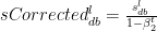
2.1. Stochastic Gradient Descent with Learning rate decay
Since in Stochastic Gradient Descent,with each epoch, we use slight different samples, the gradient descent algorithm, oscillates across the ravines and wanders around the minima, when a fixed learning rate is used. In this technique of ‘learning rate decay’ the learning rate is slowly decreased with the number of epochs and becomes smaller and smaller, so that gradient descent can take smaller steps towards the minima.
There are several techniques employed in learning rate decay
a) Exponential decay: 
b) 1/t decay : 
c) 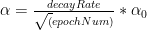
In my implementation I have used the ‘exponential decay’. The code snippet for Python is shown below
if lrDecay == True:
   learningRate = np.power(decayRate,(num_epochs/1000)) * learningRate
2.1a. Stochastic Gradient Descent with Learning rate decay – Python
import numpy as np
import matplotlib
import matplotlib.pyplot as plt
import sklearn.linear_model
import pandas as pd
import sklearn
import sklearn.datasets
exec(open("DLfunctions7.py").read())
exec(open("load_mnist.py").read())
# Read the MNIST data
training=list(read(dataset='training',path=".\\mnist"))
test=list(read(dataset='testing',path=".\\mnist"))
lbls=[]
pxls=[]
for i in range(60000):
l,p=training[i]
lbls.append(l)
pxls.append(p)
labels= np.array(lbls)
pixels=np.array(pxls)
y=labels.reshape(-1,1)
X=pixels.reshape(pixels.shape[0],-1)
X1=X.T
Y1=y.T
permutation = list(np.random.permutation(2**10))
X2 = X1[:, permutation]
Y2 = Y1[:, permutation].reshape((1,2**10))
# Set layer dimensions
layersDimensions=[784, 15,9,10]
# Perform SGD with learning rate decay
parameters = L_Layer_DeepModel_SGD(X2, Y2, layersDimensions, hiddenActivationFunc='relu',
outputActivationFunc="softmax",
learningRate = 0.01 , lrDecay=True, decayRate=0.9999,
optimizer="gd",
mini_batch_size =512, num_epochs = 1000, print_cost = True,figure="fig2.png")

2.1b. Stochastic Gradient Descent with Learning rate decay – R
source("mnist.R")
source("DLfunctions7.R")
# Read and load MNIST
load_mnist()
x <- t(train$x)
X <- x[,1:60000]
y <-train$y
y1 <- y[1:60000]
y2 <- as.matrix(y1)
Y=t(y2)
permutation = c(sample(2^10))
X1 = X[, permutation]
y1 = Y[1, permutation]
y2 <- as.matrix(y1)
Y1=t(y2)
# Set layer dimensions
layersDimensions=c(784, 15,9, 10)
retvalsSGD= L_Layer_DeepModel_SGD(X1, Y1, layersDimensions,
hiddenActivationFunc='tanh',
outputActivationFunc="softmax",
learningRate = 0.05,
lrDecay=TRUE,
decayRate=0.9999,
optimizer="gd",
mini_batch_size = 512,
num_epochs = 5000,
print_cost = True)
iterations <- seq(0,5000,1000)
costs=retvalsSGD$costs
df=data.frame(iterations,costs)
ggplot(df,aes(x=iterations,y=costs)) + geom_point() + geom_line(color="blue") +
ggtitle("Costs vs number of epochs") + xlab("No of epochs") + ylab("Cost")

2.1c. Stochastic Gradient Descent with Learning rate decay – Octave
source("DL7functions.m")
#Load and read MNIST
load('./mnist/mnist.txt.gz');
#Create a random permutatation from 1024
permutation = randperm(1024);
disp(length(permutation));

# Use this 1024 as the batch
X=trainX(permutation,:);
Y=trainY(permutation,:);

# Set layer dimensions
layersDimensions=[784, 15, 9, 10];
# Perform SGD with regular Learning rate decay
[weights biases costs]=L_Layer_DeepModel_SGD(X', Y', layersDimensions,
 hiddenActivationFunc='relu',
 outputActivationFunc="softmax",
 learningRate = 0.01,
 lrDecay=true,
 decayRate=0.999,
 lambd=0,
 keep_prob=1,
 optimizer="gd",
 beta=0.9,
 beta1=0.9,
 beta2=0.999,
 epsilon=10^-8,
 mini_batch_size = 512,
 num_epochs = 5000);
plotCostVsEpochs(5000,costs)

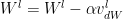
3.1. Stochastic Gradient Descent with Momentum
Stochastic Gradient Descent with Momentum uses the exponentially weighted average method discusses above and more generally moves faster into the ravine than across it. The equations are


 where
where
 and
and  are the momentum terms which are exponentially weighted with the corresponding gradients ‘dW’ and ‘db’ at the corresponding layer ‘l’ The code snippet for Stochastic Gradient Descent with momentum in R is shown below
# Perform Gradient Descent with momentum
# Input : Weights and biases
#       : beta
#       : gradients
#       : learning rate
#       : outputActivationFunc - Activation function at hidden layer sigmoid/softmax
#output : Updated weights after 1 iteration
gradientDescentWithMomentum  <- function(parameters, gradients,v, beta, learningRate,outputActivationFunc="sigmoid"){

    L = length(parameters)/2 # number of layers in the neural network
    # Update rule for each parameter. Use a for loop.
    for(l in 1:(L-1)){
        # Compute velocities
        # v['dWk'] = beta *v['dWk'] + (1-beta)*dWk
        v[[paste("dW",l, sep="")]] = beta*v[[paste("dW",l, sep="")]] +
                   (1-beta) * gradients[[paste('dW',l,sep="")]]
        v[[paste("db",l, sep="")]] = beta*v[[paste("db",l, sep="")]] +
            (1-beta) * gradients[[paste('db',l,sep="")]]

        parameters[[paste("W",l,sep="")]] = parameters[[paste("W",l,sep="")]] -
            learningRate* v[[paste("dW",l, sep="")]]
        parameters[[paste("b",l,sep="")]] = parameters[[paste("b",l,sep="")]] -
            learningRate* v[[paste("db",l, sep="")]]
    }
    # Compute for the Lth layer
    if(outputActivationFunc=="sigmoid"){
        v[[paste("dW",L, sep="")]] = beta*v[[paste("dW",L, sep="")]] +
            (1-beta) * gradients[[paste('dW',L,sep="")]]
        v[[paste("db",L, sep="")]] = beta*v[[paste("db",L, sep="")]] +
            (1-beta) * gradients[[paste('db',L,sep="")]]

        parameters[[paste("W",L,sep="")]] = parameters[[paste("W",L,sep="")]] -
            learningRate* v[[paste("dW",l, sep="")]]
        parameters[[paste("b",L,sep="")]] = parameters[[paste("b",L,sep="")]] -
            learningRate* v[[paste("db",l, sep="")]]

    }else if (outputActivationFunc=="softmax"){
        v[[paste("dW",L, sep="")]] = beta*v[[paste("dW",L, sep="")]] +
            (1-beta) * t(gradients[[paste('dW',L,sep="")]])
        v[[paste("db",L, sep="")]] = beta*v[[paste("db",L, sep="")]] +
            (1-beta) * t(gradients[[paste('db',L,sep="")]])
        parameters[[paste("W",L,sep="")]] = parameters[[paste("W",L,sep="")]] -
            learningRate* t(gradients[[paste("dW",L,sep="")]])
        parameters[[paste("b",L,sep="")]] = parameters[[paste("b",L,sep="")]] -
            learningRate* t(gradients[[paste("db",L,sep="")]])
    }
    return(parameters)
}
3.1a. Stochastic Gradient Descent with Momentum- Python
import numpy as np
import matplotlib
import matplotlib.pyplot as plt
import sklearn.linear_model
import pandas as pd
import sklearn
import sklearn.datasets
# Read and load data
exec(open("DLfunctions7.py").read())
exec(open("load_mnist.py").read())
training=list(read(dataset='training',path=".\\mnist"))
test=list(read(dataset='testing',path=".\\mnist"))
lbls=[]
pxls=[]
for i in range(60000):
l,p=training[i]
lbls.append(l)
pxls.append(p)
labels= np.array(lbls)
pixels=np.array(pxls)
y=labels.reshape(-1,1)
X=pixels.reshape(pixels.shape[0],-1)
X1=X.T
Y1=y.T
permutation = list(np.random.permutation(2**10))
X2 = X1[:, permutation]
Y2 = Y1[:, permutation].reshape((1,2**10))
layersDimensions=[784, 15,9,10]
# Perform SGD with momentum
parameters = L_Layer_DeepModel_SGD(X2, Y2, layersDimensions, hiddenActivationFunc='relu',
outputActivationFunc="softmax",learningRate = 0.01 ,
optimizer="momentum", beta=0.9,
mini_batch_size =512, num_epochs = 1000, print_cost = True,figure="fig3.png")

3.1b. Stochastic Gradient Descent with Momentum- R
source("mnist.R")
source("DLfunctions7.R")
load_mnist()
x <- t(train$x)
X <- x[,1:60000]
y <-train$y
y1 <- y[1:60000]
y2 <- as.matrix(y1)
Y=t(y2)
permutation = c(sample(2^10))
X1 = X[, permutation]
y1 = Y[1, permutation]
y2 <- as.matrix(y1)
Y1=t(y2)
layersDimensions=c(784, 15,9, 10)
# Perform SGD with momentum
retvalsSGD= L_Layer_DeepModel_SGD(X1, Y1, layersDimensions,
hiddenActivationFunc='tanh',
outputActivationFunc="softmax",
learningRate = 0.05,
optimizer="momentum",
beta=0.9,
mini_batch_size = 512,
num_epochs = 5000,
print_cost = True)
iterations <- seq(0,5000,1000)
costs=retvalsSGD$costs
df=data.frame(iterations,costs)
ggplot(df,aes(x=iterations,y=costs)) + geom_point() + geom_line(color="blue") +
ggtitle("Costs vs number of epochs") + xlab("No of epochs") + ylab("Cost")

3.1c. Stochastic Gradient Descent with Momentum- Octave
source("DL7functions.m")
#Load and read MNIST
load('./mnist/mnist.txt.gz');
#Create a random permutatation from 60K
permutation = randperm(1024);
disp(length(permutation));

# Use this 1024 as the batch
X=trainX(permutation,:);
Y=trainY(permutation,:);

# Set layer dimensions
layersDimensions=[784, 15, 9, 10];
# Perform SGD with Momentum
[weights biases costs]=L_Layer_DeepModel_SGD(X', Y', layersDimensions,
 hiddenActivationFunc='relu',
 outputActivationFunc="softmax",
 learningRate = 0.01,
 lrDecay=false,
 decayRate=1,
 lambd=0,
 keep_prob=1,
 optimizer="momentum",
 beta=0.9,
 beta1=0.9,
 beta2=0.999,
 epsilon=10^-8,
 mini_batch_size = 512,
 num_epochs = 5000);

plotCostVsEpochs(5000,costs)

4.1. Stochastic Gradient Descent with RMSProp
Stochastic Gradient Descent with RMSProp tries to move faster towards the minima while dampening the oscillations across the ravine.
The equations are


where  and
and  are the RMSProp terms which are exponentially weighted with the corresponding gradients ‘dW’ and ‘db’ at the corresponding layer ‘l’
The code snippet in Octave is shown below
# Update parameters with RMSProp
# Input : parameters
#       : gradients
#       : s
#       : beta
#       : learningRate
#       :
#output : Updated parameters RMSProp
function [weights biases] = gradientDescentWithRMSProp(weights, biases,gradsDW,gradsDB, sdW, sdB, beta1, epsilon, learningRate,outputActivationFunc="sigmoid")
    L = size(weights)(2); # number of layers in the neural network
    # Update rule for each parameter.
    for l=1:(L-1)
        sdW{l} =  beta1*sdW{l} + (1 -beta1) * gradsDW{l} .* gradsDW{l};
        sdB{l} =  beta1*sdB{l} + (1 -beta1) * gradsDB{l} .* gradsDB{l};
        weights{l} = weights{l} - learningRate* gradsDW{l} ./ sqrt(sdW{l} + epsilon);
        biases{l} = biases{l} -  learningRate* gradsDB{l} ./ sqrt(sdB{l} + epsilon);
    endfor

    if (strcmp(outputActivationFunc,"sigmoid"))
        sdW{L} =  beta1*sdW{L} + (1 -beta1) * gradsDW{L} .* gradsDW{L};
        sdB{L} =  beta1*sdB{L} + (1 -beta1) * gradsDB{L} .* gradsDB{L};
        weights{L} = weights{L} -learningRate* gradsDW{L} ./ sqrt(sdW{L} +epsilon);
        biases{L} = biases{L} -learningRate* gradsDB{L} ./ sqrt(sdB{L} + epsilon);
     elseif (strcmp(outputActivationFunc,"softmax"))
        sdW{L} =  beta1*sdW{L} + (1 -beta1) * gradsDW{L}' .* gradsDW{L}';
        sdB{L} =  beta1*sdB{L} + (1 -beta1) * gradsDB{L}' .* gradsDB{L}';
        weights{L} = weights{L} -learningRate* gradsDW{L}' ./ sqrt(sdW{L} +epsilon);
        biases{L} = biases{L} -learningRate* gradsDB{L}' ./ sqrt(sdB{L} + epsilon);
     endif
end
4.1a. Stochastic Gradient Descent with RMSProp – Python
import numpy as np
import matplotlib
import matplotlib.pyplot as plt
import sklearn.linear_model
import pandas as pd
import sklearn
import sklearn.datasets
exec(open("DLfunctions7.py").read())
exec(open("load_mnist.py").read())
# Read and load MNIST
training=list(read(dataset='training',path=".\\mnist"))
test=list(read(dataset='testing',path=".\\mnist"))
lbls=[]
pxls=[]
for i in range(60000):
l,p=training[i]
lbls.append(l)
pxls.append(p)
labels= np.array(lbls)
pixels=np.array(pxls)
y=labels.reshape(-1,1)
X=pixels.reshape(pixels.shape[0],-1)
X1=X.T
Y1=y.T
print("X1=",X1.shape)
print("y1=",Y1.shape)
permutation = list(np.random.permutation(2**10))
X2 = X1[:, permutation]
Y2 = Y1[:, permutation].reshape((1,2**10))
layersDimensions=[784, 15,9,10]
# Use SGD with RMSProp
parameters = L_Layer_DeepModel_SGD(X2, Y2, layersDimensions, hiddenActivationFunc='relu',
outputActivationFunc="softmax",learningRate = 0.01 ,
optimizer="rmsprop", beta1=0.7, epsilon=1e-8,
mini_batch_size =512, num_epochs = 1000, print_cost = True,figure="fig4.png")

4.1b. Stochastic Gradient Descent with RMSProp – R
source("mnist.R")
source("DLfunctions7.R")
load_mnist()
x <- t(train$x)
X <- x[,1:60000]
y <-train$y
y1 <- y[1:60000]
y2 <- as.matrix(y1)
Y=t(y2)
permutation = c(sample(2^10))
X1 = X[, permutation]
y1 = Y[1, permutation]
y2 <- as.matrix(y1)
Y1=t(y2)
layersDimensions=c(784, 15,9, 10)
#Perform SGD with RMSProp
retvalsSGD= L_Layer_DeepModel_SGD(X1, Y1, layersDimensions,
hiddenActivationFunc='tanh',
outputActivationFunc="softmax",
learningRate = 0.001,
optimizer="rmsprop",
beta1=0.9,
epsilon=10^-8,
mini_batch_size = 512,
num_epochs = 5000 ,
print_cost = True)
iterations <- seq(0,5000,1000)
costs=retvalsSGD$costs
df=data.frame(iterations,costs)
ggplot(df,aes(x=iterations,y=costs)) + geom_point() + geom_line(color="blue") +
ggtitle("Costs vs number of epochs") + xlab("No of epochs") + ylab("Cost")

4.1c. Stochastic Gradient Descent with RMSProp – Octave
source("DL7functions.m")
load('./mnist/mnist.txt.gz');
#Create a random permutatation from 1024
permutation = randperm(1024);

# Use this 1024 as the batch
X=trainX(permutation,:);
Y=trainY(permutation,:);

# Set layer dimensions
layersDimensions=[784, 15, 9, 10];
#Perform SGD with RMSProp
[weights biases costs]=L_Layer_DeepModel_SGD(X', Y', layersDimensions,
 hiddenActivationFunc='relu',
 outputActivationFunc="softmax",
 learningRate = 0.005,
 lrDecay=false,
 decayRate=1,
 lambd=0,
 keep_prob=1,
 optimizer="rmsprop",
 beta=0.9,
 beta1=0.9,
 beta2=0.999,
 epsilon=1,
 mini_batch_size = 512,
 num_epochs = 5000);
plotCostVsEpochs(5000,costs)

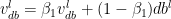
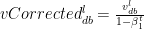
5.1. Stochastic Gradient Descent with Adam
Adaptive Moment Estimate is a combination of the momentum (1st moment) and RMSProp(2nd moment). The equations for Adam are below

The bias corrections for the 1st moment

Similarly the moving average for the 2nd moment- RMSProp


The bias corrections for the 2nd moment

The Adam Gradient Descent is given by


The code snippet of Adam in R is included below
# Perform Gradient Descent with Adam
# Input : Weights and biases
#       : beta1
#       : epsilon
#       : gradients
#       : learning rate
#       : outputActivationFunc - Activation function at hidden layer sigmoid/softmax
#output : Updated weights after 1 iteration
gradientDescentWithAdam  <- function(parameters, gradients,v, s, t,
                        beta1=0.9, beta2=0.999, epsilon=10^-8, learningRate=0.1,outputActivationFunc="sigmoid"){

    L = length(parameters)/2 # number of layers in the neural network
    v_corrected <- list()
    s_corrected <- list()
    # Update rule for each parameter. Use a for loop.
    for(l in 1:(L-1)){
        # v['dWk'] = beta *v['dWk'] + (1-beta)*dWk
        v[[paste("dW",l, sep="")]] = beta1*v[[paste("dW",l, sep="")]] +
            (1-beta1) * gradients[[paste('dW',l,sep="")]]
        v[[paste("db",l, sep="")]] = beta1*v[[paste("db",l, sep="")]] +
            (1-beta1) * gradients[[paste('db',l,sep="")]]


        # Compute bias-corrected first moment estimate.
        v_corrected[[paste("dW",l, sep="")]] = v[[paste("dW",l, sep="")]]/(1-beta1^t)
        v_corrected[[paste("db",l, sep="")]] = v[[paste("db",l, sep="")]]/(1-beta1^t)

        # Element wise multiply of gradients
        s[[paste("dW",l, sep="")]] = beta2*s[[paste("dW",l, sep="")]] +
            (1-beta2) * gradients[[paste('dW',l,sep="")]] * gradients[[paste('dW',l,sep="")]]
        s[[paste("db",l, sep="")]] = beta2*s[[paste("db",l, sep="")]] +
            (1-beta2) * gradients[[paste('db',l,sep="")]] * gradients[[paste('db',l,sep="")]]

        # Compute bias-corrected second moment estimate.
        s_corrected[[paste("dW",l, sep="")]] = s[[paste("dW",l, sep="")]]/(1-beta2^t)
        s_corrected[[paste("db",l, sep="")]] = s[[paste("db",l, sep="")]]/(1-beta2^t)

        # Update parameters.
        d1=sqrt(s_corrected[[paste("dW",l, sep="")]]+epsilon)
        d2=sqrt(s_corrected[[paste("db",l, sep="")]]+epsilon)

        parameters[[paste("W",l,sep="")]] = parameters[[paste("W",l,sep="")]] -
            learningRate * v_corrected[[paste("dW",l, sep="")]]/d1
        parameters[[paste("b",l,sep="")]] = parameters[[paste("b",l,sep="")]] -
            learningRate*v_corrected[[paste("db",l, sep="")]]/d2
    }
    # Compute for the Lth layer
    if(outputActivationFunc=="sigmoid"){
        v[[paste("dW",L, sep="")]] = beta1*v[[paste("dW",L, sep="")]] +
            (1-beta1) * gradients[[paste('dW',L,sep="")]]
        v[[paste("db",L, sep="")]] = beta1*v[[paste("db",L, sep="")]] +
            (1-beta1) * gradients[[paste('db',L,sep="")]]

        # Compute bias-corrected first moment estimate.
        v_corrected[[paste("dW",L, sep="")]] = v[[paste("dW",L, sep="")]]/(1-beta1^t)
        v_corrected[[paste("db",L, sep="")]] = v[[paste("db",L, sep="")]]/(1-beta1^t)

        # Element wise multiply of gradients
        s[[paste("dW",L, sep="")]] = beta2*s[[paste("dW",L, sep="")]] +
            (1-beta2) * gradients[[paste('dW',L,sep="")]] * gradients[[paste('dW',L,sep="")]]
        s[[paste("db",L, sep="")]] = beta2*s[[paste("db",L, sep="")]] +
            (1-beta2) * gradients[[paste('db',L,sep="")]] * gradients[[paste('db',L,sep="")]]

        # Compute bias-corrected second moment estimate.
        s_corrected[[paste("dW",L, sep="")]] = s[[paste("dW",L, sep="")]]/(1-beta2^t)
        s_corrected[[paste("db",L, sep="")]] = s[[paste("db",L, sep="")]]/(1-beta2^t)

        # Update parameters.
        d1=sqrt(s_corrected[[paste("dW",L, sep="")]]+epsilon)
        d2=sqrt(s_corrected[[paste("db",L, sep="")]]+epsilon)

        parameters[[paste("W",L,sep="")]] = parameters[[paste("W",L,sep="")]] -
            learningRate * v_corrected[[paste("dW",L, sep="")]]/d1
        parameters[[paste("b",L,sep="")]] = parameters[[paste("b",L,sep="")]] -
            learningRate*v_corrected[[paste("db",L, sep="")]]/d2

    }else if (outputActivationFunc=="softmax"){
        v[[paste("dW",L, sep="")]] = beta1*v[[paste("dW",L, sep="")]] +
            (1-beta1) * t(gradients[[paste('dW',L,sep="")]])
        v[[paste("db",L, sep="")]] = beta1*v[[paste("db",L, sep="")]] +
            (1-beta1) * t(gradients[[paste('db',L,sep="")]])

        # Compute bias-corrected first moment estimate.
        v_corrected[[paste("dW",L, sep="")]] = v[[paste("dW",L, sep="")]]/(1-beta1^t)
        v_corrected[[paste("db",L, sep="")]] = v[[paste("db",L, sep="")]]/(1-beta1^t)

        # Element wise multiply of gradients
        s[[paste("dW",L, sep="")]] = beta2*s[[paste("dW",L, sep="")]] +
            (1-beta2) * t(gradients[[paste('dW',L,sep="")]]) * t(gradients[[paste('dW',L,sep="")]])
        s[[paste("db",L, sep="")]] = beta2*s[[paste("db",L, sep="")]] +
            (1-beta2) * t(gradients[[paste('db',L,sep="")]]) * t(gradients[[paste('db',L,sep="")]])

        # Compute bias-corrected second moment estimate.
        s_corrected[[paste("dW",L, sep="")]] = s[[paste("dW",L, sep="")]]/(1-beta2^t)
        s_corrected[[paste("db",L, sep="")]] = s[[paste("db",L, sep="")]]/(1-beta2^t)

        # Update parameters.
        d1=sqrt(s_corrected[[paste("dW",L, sep="")]]+epsilon)
        d2=sqrt(s_corrected[[paste("db",L, sep="")]]+epsilon)

        parameters[[paste("W",L,sep="")]] = parameters[[paste("W",L,sep="")]] -
            learningRate * v_corrected[[paste("dW",L, sep="")]]/d1
        parameters[[paste("b",L,sep="")]] = parameters[[paste("b",L,sep="")]] -
            learningRate*v_corrected[[paste("db",L, sep="")]]/d2
    }
    return(parameters)
}
5.1a. Stochastic Gradient Descent with Adam – Python
import numpy as np
import matplotlib
import matplotlib.pyplot as plt
import sklearn.linear_model
import pandas as pd
import sklearn
import sklearn.datasets
exec(open("DLfunctions7.py").read())
exec(open("load_mnist.py").read())
training=list(read(dataset='training',path=".\\mnist"))
test=list(read(dataset='testing',path=".\\mnist"))
lbls=[]
pxls=[]
print(len(training))
for i in range(60000):
l,p=training[i]
lbls.append(l)
pxls.append(p)
labels= np.array(lbls)
pixels=np.array(pxls)
y=labels.reshape(-1,1)
X=pixels.reshape(pixels.shape[0],-1)
X1=X.T
Y1=y.T
permutation = list(np.random.permutation(2**10))
X2 = X1[:, permutation]
Y2 = Y1[:, permutation].reshape((1,2**10))
layersDimensions=[784, 15,9,10]
#Perform SGD with Adam optimization
parameters = L_Layer_DeepModel_SGD(X2, Y2, layersDimensions, hiddenActivationFunc='relu',
outputActivationFunc="softmax",learningRate = 0.01 ,
optimizer="adam", beta1=0.9, beta2=0.9, epsilon = 1e-8,
mini_batch_size =512, num_epochs = 1000, print_cost = True, figure="fig5.png")

5.1b. Stochastic Gradient Descent with Adam – R
source("mnist.R")
source("DLfunctions7.R")
load_mnist()
x <- t(train$x)
X <- x[,1:60000]
y <-train$y
y1 <- y[1:60000]
y2 <- as.matrix(y1)
Y=t(y2)
permutation = c(sample(2^10))
X1 = X[, permutation]
y1 = Y[1, permutation]
y2 <- as.matrix(y1)
Y1=t(y2)
layersDimensions=c(784, 15,9, 10)
#Perform SGD with Adam
retvalsSGD= L_Layer_DeepModel_SGD(X1, Y1, layersDimensions,
hiddenActivationFunc='tanh',
outputActivationFunc="softmax",
learningRate = 0.005,
optimizer="adam",
beta1=0.7,
beta2=0.9,
epsilon=10^-8,
mini_batch_size = 512,
num_epochs = 5000 ,
print_cost = True)
iterations <- seq(0,5000,1000)
costs=retvalsSGD$costs
df=data.frame(iterations,costs)
ggplot(df,aes(x=iterations,y=costs)) + geom_point() + geom_line(color="blue") +
ggtitle("Costs vs number of epochs") + xlab("No of epochs") + ylab("Cost")

5.1c. Stochastic Gradient Descent with Adam – Octave
source("DL7functions.m")
load('./mnist/mnist.txt.gz');
#Create a random permutatation from 1024
permutation = randperm(1024);
disp(length(permutation));

# Use this 1024 as the batch
X=trainX(permutation,:);
Y=trainY(permutation,:);
# Set layer dimensions
layersDimensions=[784, 15, 9, 10];

# Note the high value for epsilon.
#Otherwise GD with Adam does not seem to converge
# Perform SGD with Adam
[weights biases costs]=L_Layer_DeepModel_SGD(X', Y', layersDimensions,
                       hiddenActivationFunc='relu',
                       outputActivationFunc="softmax",
                       learningRate = 0.1,
                       lrDecay=false,
                       decayRate=1,
                       lambd=0,
                       keep_prob=1,
                       optimizer="adam",
                       beta=0.9,
                       beta1=0.9,
                       beta2=0.9,
                       epsilon=100,
                       mini_batch_size = 512,
                       num_epochs = 5000);
plotCostVsEpochs(5000,costs)

Conclusion: In this post I discuss and implement several Stochastic Gradient Descent optimization methods. The implementation of these methods enhance my already existing generic L-Layer Deep Learning Network implementation in vectorized Python, R and Octave, which I had discussed in the previous post in this series on Deep Learning from first principles in Python, R and Octave. Check it out, if you haven’t already. As already mentioned the code for this post can be cloned/forked from Github at DeepLearning-Part7
Watch this space! I’ll be back!
Also see
1.My book ‘Practical Machine Learning with R and Python’ on Amazon
2. Deep Learning from first principles in Python, R and Octave – Part 3
3. Experiments with deblurring using OpenCV
3. Design Principles of Scalable, Distributed Systems
4. Natural language processing: What would Shakespeare say?
5. yorkr crashes the IPL party! – Part 3!
6. cricketr flexes new muscles: The final analysis
To see all post click Index of posts


 by doing
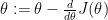 .
.
 be a function that computes the derivative
  . Gradient Checking allows us to numerically evaluate the implementation of the function
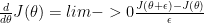
 as opposed
  for the 1-sided derivative.
 by bumping up
  (
( )
)
 by bumping down

 or ‘gradapprox’ as
 using the 2 sided derivative.
 or
or  the implementation is correct. In the
  -learning rate
 – 0.9
– 0.9 and
and 


 and
and 
 and
and 
 and
and 


 . It can be shown that
 see equation 2 in
  see equation (f) in
  because
  -(1a)
-(1a) -(1b)
-(1b) -(1c)
-(1c)
 -(1d)
-(1d)
 – (2a)
 – (2b)
 – (2c)
 – (2d)
 and
and 


 = a g’(z) = a(1-a) – See
 , …
, … ![v_{L-1}]](https://s0.wp.com/latex.php?latex=v_%7BL-1%7D%5D&bg=ffffff&fg=000000&s=0&c=20201002)
 , …
, … 
 …
… ![v_{L}]](https://s0.wp.com/latex.php?latex=v_%7BL%7D%5D&bg=ffffff&fg=000000&s=0&c=20201002)
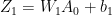
 is the number of activation units in each hidden layer, which is specified while actually executing the Deep Learning network using the function L_Layer_DeepModel(), in all the implementations Python, R and Octave


 =
= 


 and
and  -(a) and
 and
and 
 and
and  (b)
(b) -(c)
-(c) and using (b) we get


 -(d)
-(d)

 see
see 


 -(A)
-(A) -(B)
-(B)

 -(C)
-(C)
 -(D)
-(D) – From (C)
 – From (D)
 – From (A)
 – From (B)


