This is the 4th installment of my ‘Practical Machine Learning with R and Python’ series. In this part I discuss classification with Support Vector Machines (SVMs), using both a Linear and a Radial basis kernel, and Decision Trees. Further, a closer look is taken at some of the metrics associated with binary classification, namely accuracy vs precision and recall. I also touch upon Validation curves, Precision-Recall, ROC curves and AUC with equivalent code in R and Python
This post is a continuation of my 3 earlier posts on Practical Machine Learning in R and Python
1. Practical Machine Learning with R and Python – Part 1
2. Practical Machine Learning with R and Python – Part 2
3. Practical Machine Learning with R and Python – Part 3
The RMarkdown file with the code and the associated data files can be downloaded from Github at MachineLearning-RandPython-Part4
Note: Please listen to my video presentations Machine Learning in youtube
1. Machine Learning in plain English-Part 1
2. Machine Learning in plain English-Part 2
3. Machine Learning in plain English-Part 3
Check out my compact and minimal book “Practical Machine Learning with R and Python:Third edition- Machine Learning in stereo” available in Amazon in paperback($12.99) and kindle($8.99) versions. My book includes implementations of key ML algorithms and associated measures and metrics. The book is ideal for anybody who is familiar with the concepts and would like a quick reference to the different ML algorithms that can be applied to problems and how to select the best model. Pick your copy today!!

Support Vector Machines (SVM) are another useful Machine Learning model that can be used for both regression and classification problems. SVMs used in classification, compute the hyperplane, that separates the 2 classes with the maximum margin. To do this the features may be transformed into a larger multi-dimensional feature space. SVMs can be used with different kernels namely linear, polynomial or radial basis to determine the best fitting model for a given classification problem.
In the 2nd part of this series Practical Machine Learning with R and Python – Part 2, I had mentioned the various metrics that are used in classification ML problems namely Accuracy, Precision, Recall and F1 score. Accuracy gives the fraction of data that were correctly classified as belonging to the +ve or -ve class. However ‘accuracy’ in itself is not a good enough measure because it does not take into account the fraction of the data that were incorrectly classified. This issue becomes even more critical in different domains. For e.g a surgeon who would like to detect cancer, would like to err on the side of caution, and classify even a possibly non-cancerous patient as possibly having cancer, rather than mis-classifying a malignancy as benign. Here we would like to increase recall or sensitivity which is given by Recall= TP/(TP+FN) or we try reduce mis-classification by either increasing the (true positives) TP or reducing (false negatives) FN
On the other hand, search algorithms would like to increase precision which tries to reduce the number of irrelevant results in the search result. Precision= TP/(TP+FP). In other words we do not want ‘false positives’ or irrelevant results to come in the search results and there is a need to reduce the false positives.
When we try to increase ‘precision’, we do so at the cost of ‘recall’, and vice-versa. I found this diagram and explanation in Wikipedia very useful Source: Wikipedia
“Consider a brain surgeon tasked with removing a cancerous tumor from a patient’s brain. The surgeon needs to remove all of the tumor cells since any remaining cancer cells will regenerate the tumor. Conversely, the surgeon must not remove healthy brain cells since that would leave the patient with impaired brain function. The surgeon may be more liberal in the area of the brain she removes to ensure she has extracted all the cancer cells. This decision increases recall but reduces precision. On the other hand, the surgeon may be more conservative in the brain she removes to ensure she extracts only cancer cells. This decision increases precision but reduces recall. That is to say, greater recall increases the chances of removing healthy cells (negative outcome) and increases the chances of removing all cancer cells (positive outcome). Greater precision decreases the chances of removing healthy cells (positive outcome) but also decreases the chances of removing all cancer cells (negative outcome).”

1.1a. Linear SVM – R code
In R code below I use SVM with linear kernel
source('RFunctions-1.R')
library(dplyr)
library(e1071)
library(caret)
library(reshape2)
library(ggplot2)
# Read data. Data from SKLearn
cancer <- read.csv("cancer.csv")
cancer$target <- as.factor(cancer$target)
# Split into training and test sets
train_idx <- trainTestSplit(cancer,trainPercent=75,seed=5)
train <- cancer[train_idx, ]
test <- cancer[-train_idx, ]
# Fit a linear basis kernel. DO not scale the data
svmfit=svm(target~., data=train, kernel="linear",scale=FALSE)
ypred=predict(svmfit,test)
#Print a confusion matrix
confusionMatrix(ypred,test$target)## Confusion Matrix and Statistics
##
## Reference
## Prediction 0 1
## 0 54 3
## 1 3 82
##
## Accuracy : 0.9577
## 95% CI : (0.9103, 0.9843)
## No Information Rate : 0.5986
## P-Value [Acc > NIR] : <2e-16
##
## Kappa : 0.9121
## Mcnemar's Test P-Value : 1
##
## Sensitivity : 0.9474
## Specificity : 0.9647
## Pos Pred Value : 0.9474
## Neg Pred Value : 0.9647
## Prevalence : 0.4014
## Detection Rate : 0.3803
## Detection Prevalence : 0.4014
## Balanced Accuracy : 0.9560
##
## 'Positive' Class : 0
## 1.1b Linear SVM – Python code
The code below creates a SVM with linear basis in Python and also dumps the corresponding classification metrics
import numpy as np
import pandas as pd
import os
import matplotlib.pyplot as plt
from sklearn.model_selection import train_test_split
from sklearn.svm import LinearSVC

from sklearn.datasets import make_classification, make_blobs

from sklearn.metrics import confusion_matrix
from matplotlib.colors import ListedColormap
from sklearn.datasets import load_breast_cancer
# Load the cancer data
(X_cancer, y_cancer) = load_breast_cancer(return_X_y = True)
X_train, X_test, y_train, y_test = train_test_split(X_cancer, y_cancer,
                                                   random_state = 0)
clf = LinearSVC().fit(X_train, y_train)
print('Breast cancer dataset')
print('Accuracy of Linear SVC classifier on training set: {:.2f}'
     .format(clf.score(X_train, y_train)))
print('Accuracy of Linear SVC classifier on test set: {:.2f}'
     .format(clf.score(X_test, y_test)))
## Breast cancer dataset
## Accuracy of Linear SVC classifier on training set: 0.92
## Accuracy of Linear SVC classifier on test set: 0.941.2 Dummy classifier
Often when we perform classification tasks using any ML model namely logistic regression, SVM, neural networks etc. it is very useful to determine how well the ML model performs agains at dummy classifier. A dummy classifier uses some simple computation like frequency of majority class, instead of fitting and ML model. It is essential that our ML model does much better that the dummy classifier. This problem is even more important in imbalanced classes where we have only about 10% of +ve samples. If any ML model we create has a accuracy of about 0.90 then it is evident that our classifier is not doing any better than a dummy classsfier which can just take a majority count of this imbalanced class and also come up with 0.90. We need to be able to do better than that.
In the examples below (1.3a & 1.3b) it can be seen that SVMs with ‘radial basis’ kernel with unnormalized data, for both R and Python, do not perform any better than the dummy classifier.
1.2a Dummy classifier – R code
R does not seem to have an explicit dummy classifier. I created a simple dummy classifier that predicts the majority class. SKlearn in Python also includes other strategies like uniform, stratified etc. but this should be possible to create in R also.
# Create a simple dummy classifier that computes the ratio of the majority class to the totla
DummyClassifierAccuracy <- function(train,test,type="majority"){
  if(type=="majority"){
      count <- sum(train$target==1)/dim(train)[1]
  }
  count
}


cancer <- read.csv("cancer.csv")
cancer$target <- as.factor(cancer$target)

# Create training and test sets
train_idx <- trainTestSplit(cancer,trainPercent=75,seed=5)
train <- cancer[train_idx, ]
test <- cancer[-train_idx, ]

#Dummy classifier majority class
acc=DummyClassifierAccuracy(train,test)
sprintf("Accuracy is %f",acc)
## [1] "Accuracy is 0.638498"1.2b Dummy classifier – Python code
This dummy classifier uses the majority class.
import numpy as np
import pandas as pd
import os
import matplotlib.pyplot as plt
from sklearn.datasets import load_breast_cancer
from sklearn.model_selection import train_test_split
from sklearn.dummy import DummyClassifier
from sklearn.metrics import confusion_matrix
(X_cancer, y_cancer) = load_breast_cancer(return_X_y = True)
X_train, X_test, y_train, y_test = train_test_split(X_cancer, y_cancer,
                                                   random_state = 0)

# Negative class (0) is most frequent
dummy_majority = DummyClassifier(strategy = 'most_frequent').fit(X_train, y_train)
y_dummy_predictions = dummy_majority.predict(X_test)

print('Dummy classifier accuracy on test set: {:.2f}'
     .format(dummy_majority.score(X_test, y_test)))
## Dummy classifier accuracy on test set: 0.631.3a – Radial SVM (un-normalized) – R code
SVMs perform better when the data is normalized or scaled. The 2 examples below show that SVM with radial basis kernel does not perform any better than the dummy classifier
library(dplyr)
library(e1071)
library(caret)
library(reshape2)
library(ggplot2)

# Radial SVM unnormalized
train_idx <- trainTestSplit(cancer,trainPercent=75,seed=5)
train <- cancer[train_idx, ]
test <- cancer[-train_idx, ]
# Unnormalized data
svmfit=svm(target~., data=train, kernel="radial",cost=10,scale=FALSE)
ypred=predict(svmfit,test)
confusionMatrix(ypred,test$target)
## Confusion Matrix and Statistics
##
## Reference
## Prediction 0 1
## 0 0 0
## 1 57 85
##
## Accuracy : 0.5986
## 95% CI : (0.5131, 0.6799)
## No Information Rate : 0.5986
## P-Value [Acc > NIR] : 0.5363
##
## Kappa : 0
## Mcnemar's Test P-Value : 1.195e-13
##
## Sensitivity : 0.0000
## Specificity : 1.0000
## Pos Pred Value : NaN
## Neg Pred Value : 0.5986
## Prevalence : 0.4014
## Detection Rate : 0.0000
## Detection Prevalence : 0.0000
## Balanced Accuracy : 0.5000
##
## 'Positive' Class : 0
## 1.4b – Radial SVM (un-normalized) – Python code
import numpy as np
import pandas as pd
import os
import matplotlib.pyplot as plt
from sklearn.datasets import load_breast_cancer
from sklearn.model_selection import train_test_split
from sklearn.svm import SVC

# Load the cancer data
(X_cancer, y_cancer) = load_breast_cancer(return_X_y = True)
X_train, X_test, y_train, y_test = train_test_split(X_cancer, y_cancer,
                                                   random_state = 0)


clf = SVC(C=10).fit(X_train, y_train)
print('Breast cancer dataset (unnormalized features)')
print('Accuracy of RBF-kernel SVC on training set: {:.2f}'
     .format(clf.score(X_train, y_train)))
print('Accuracy of RBF-kernel SVC on test set: {:.2f}'
     .format(clf.score(X_test, y_test)))
## Breast cancer dataset (unnormalized features)
## Accuracy of RBF-kernel SVC on training set: 1.00
## Accuracy of RBF-kernel SVC on test set: 0.631.5a – Radial SVM (Normalized) -R Code
The data is scaled (normalized ) before using the SVM model. The SVM model has 2 paramaters a) C – Large C (less regularization), more regularization b) gamma – Small gamma has larger decision boundary with more misclassfication, and larger gamma has tighter decision boundary
The R code below computes the accuracy as the regularization paramater is changed
trainingAccuracy <- NULL
testAccuracy <- NULL
C1 <- c(.01,.1, 1, 10, 20)
for(i in  C1){

    svmfit=svm(target~., data=train, kernel="radial",cost=i,scale=TRUE)
    ypredTrain <-predict(svmfit,train)
    ypredTest=predict(svmfit,test)
    a <-confusionMatrix(ypredTrain,train$target)
    b <-confusionMatrix(ypredTest,test$target)
    trainingAccuracy <-c(trainingAccuracy,a$overall[1])
    testAccuracy <-c(testAccuracy,b$overall[1])

}
print(trainingAccuracy)
## Accuracy Accuracy Accuracy Accuracy Accuracy
## 0.6384977 0.9671362 0.9906103 0.9976526 1.0000000print(testAccuracy)## Accuracy Accuracy Accuracy Accuracy Accuracy
## 0.5985915 0.9507042 0.9647887 0.9507042 0.9507042a <-rbind(C1,as.numeric(trainingAccuracy),as.numeric(testAccuracy))
b <- data.frame(t(a))
names(b) <- c("C1","trainingAccuracy","testAccuracy")
df <- melt(b,id="C1")
ggplot(df) + geom_line(aes(x=C1, y=value, colour=variable),size=2) +
xlab("C (SVC regularization)value") + ylab("Accuracy") +
ggtitle("Training and test accuracy vs C(regularization)")
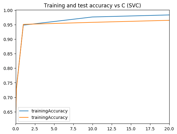
1.5b – Radial SVM (normalized) – Python
The Radial basis kernel is used on normalized data for a range of ‘C’ values and the result is plotted.
import numpy as np
import pandas as pd
import os
import matplotlib.pyplot as plt
from sklearn.datasets import load_breast_cancer
from sklearn.model_selection import train_test_split
from sklearn.svm import SVC
from sklearn.preprocessing import MinMaxScaler
scaler = MinMaxScaler()

# Load the cancer data
(X_cancer, y_cancer) = load_breast_cancer(return_X_y = True)
X_train, X_test, y_train, y_test = train_test_split(X_cancer, y_cancer,
                                                   random_state = 0)
X_train_scaled = scaler.fit_transform(X_train)
X_test_scaled = scaler.transform(X_test)

print('Breast cancer dataset (normalized with MinMax scaling)')
trainingAccuracy=[]
testAccuracy=[]
for C1 in [.01,.1, 1, 10, 20]:
    clf = SVC(C=C1).fit(X_train_scaled, y_train)
    acctrain=clf.score(X_train_scaled, y_train)
    accTest=clf.score(X_test_scaled, y_test)
    trainingAccuracy.append(acctrain)
    testAccuracy.append(accTest)

# Create a dataframe
C1=[.01,.1, 1, 10, 20]
trainingAccuracy=pd.DataFrame(trainingAccuracy,index=C1)
testAccuracy=pd.DataFrame(testAccuracy,index=C1)

# Plot training and test R squared as a function of alpha
df=pd.concat([trainingAccuracy,testAccuracy],axis=1)
df.columns=['trainingAccuracy','trainingAccuracy']

fig1=df.plot()
fig1=plt.title('Training and test accuracy vs C (SVC)')
fig1.figure.savefig('fig1.png', bbox_inches='tight')
## Breast cancer dataset (normalized with MinMax scaling)Output image:
1.6a Validation curve – R code
Sklearn includes code creating validation curves by varying paramaters and computing and plotting accuracy as gamma or C or changd. I did not find this R but I think this is a useful function and so I have created the R equivalent of this.
# The R equivalent of np.logspace
seqLogSpace <- function(start,stop,len){
  a=seq(log10(10^start),log10(10^stop),length=len)
  10^a
}

# Read the data. This is taken the SKlearn cancer data
cancer <- read.csv("cancer.csv")
cancer$target <- as.factor(cancer$target)

set.seed(6)

# Create the range of C1 in log space
param_range = seqLogSpace(-3,2,20)
# Initialize the overall training and test accuracy to NULL
overallTrainAccuracy <- NULL
overallTestAccuracy <- NULL

# Loop over the parameter range of Gamma
for(i in param_range){
    # Set no of folds
    noFolds=5
    # Create the rows which fall into different folds from 1..noFolds
    folds = sample(1:noFolds, nrow(cancer), replace=TRUE)
    # Initialize the training and test accuracy of folds to 0
    trainingAccuracy <- 0
    testAccuracy <- 0

    # Loop through the folds
    for(j in 1:noFolds){
        # The training is all rows for which the row is != j (k-1 folds -> training)
        train <- cancer[folds!=j,]
        # The rows which have j as the index become the test set
        test <- cancer[folds==j,]
        # Create a SVM model for this
        svmfit=svm(target~., data=train, kernel="radial",gamma=i,scale=TRUE)

        # Add up all the fold accuracy for training and test separately
        ypredTrain <-predict(svmfit,train)
        ypredTest=predict(svmfit,test)

        # Create confusion matrix
        a <-confusionMatrix(ypredTrain,train$target)
        b <-confusionMatrix(ypredTest,test$target)
        # Get the accuracy
        trainingAccuracy <-trainingAccuracy + a$overall[1]
        testAccuracy <-testAccuracy+b$overall[1]

    }
    # Compute the average of accuracy for K folds for number of features 'i'
    overallTrainAccuracy=c(overallTrainAccuracy,trainingAccuracy/noFolds)
    overallTestAccuracy=c(overallTestAccuracy,testAccuracy/noFolds)
}
#Create a dataframe
a <- rbind(param_range,as.numeric(overallTrainAccuracy),
               as.numeric(overallTestAccuracy))
b <- data.frame(t(a))
names(b) <- c("C1","trainingAccuracy","testAccuracy")
df <- melt(b,id="C1")
#Plot in log axis
ggplot(df) + geom_line(aes(x=C1, y=value, colour=variable),size=2) +
      xlab("C (SVC regularization)value") + ylab("Accuracy") +
      ggtitle("Training and test accuracy vs C(regularization)") + scale_x_log10()
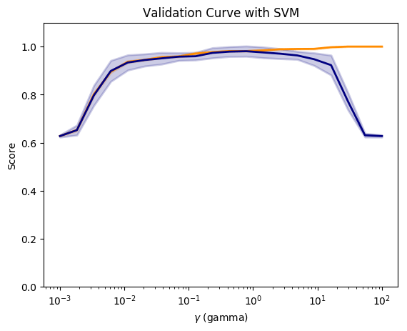
1.6b Validation curve – Python
Compute and plot the validation curve as gamma is varied.
import numpy as np
import pandas as pd
import os
import matplotlib.pyplot as plt
from sklearn.datasets import load_breast_cancer
from sklearn.model_selection import train_test_split
from sklearn.preprocessing import MinMaxScaler
from sklearn.svm import SVC
from sklearn.model_selection import validation_curve


# Load the cancer data
(X_cancer, y_cancer) = load_breast_cancer(return_X_y = True)
scaler = MinMaxScaler()
X_scaled = scaler.fit_transform(X_cancer)

# Create a gamma values from 10^-3 to 10^2 with 20 equally spaced intervals
param_range = np.logspace(-3, 2, 20)
# Compute the validation curve
train_scores, test_scores = validation_curve(SVC(), X_scaled, y_cancer,
                                            param_name='gamma',
                                            param_range=param_range, cv=10)

#Plot the figure
fig2=plt.figure()

#Compute the mean
train_scores_mean = np.mean(train_scores, axis=1)
train_scores_std = np.std(train_scores, axis=1)
test_scores_mean = np.mean(test_scores, axis=1)
test_scores_std = np.std(test_scores, axis=1)

fig2=plt.title('Validation Curve with SVM')
fig2=plt.xlabel('$\gamma$ (gamma)')
fig2=plt.ylabel('Score')
fig2=plt.ylim(0.0, 1.1)
lw = 2

fig2=plt.semilogx(param_range, train_scores_mean, label='Training score',
            color='darkorange', lw=lw)

fig2=plt.fill_between(param_range, train_scores_mean - train_scores_std,
                train_scores_mean + train_scores_std, alpha=0.2,
                color='darkorange', lw=lw)

fig2=plt.semilogx(param_range, test_scores_mean, label='Cross-validation score',
            color='navy', lw=lw)

fig2=plt.fill_between(param_range, test_scores_mean - test_scores_std,
                test_scores_mean + test_scores_std, alpha=0.2,
                color='navy', lw=lw)
fig2.figure.savefig('fig2.png', bbox_inches='tight')
Output image:
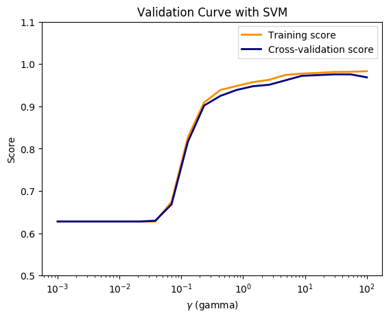
1.7a Validation Curve (Preventing data leakage) – Python code
In this course Applied Machine Learning in Python, the Professor states that when we apply the same data transformation to a entire dataset, it will cause a data leakage. “The proper way to do cross-validation when you need to scale the data is not to scale the entire dataset with a single transform, since this will indirectly leak information into the training data about the whole dataset, including the test data (see the lecture on data leakage later in the course). Instead, scaling/normalizing must be computed and applied for each cross-validation fold separately”
So I apply separate scaling to the training and testing folds and plot. In the lecture the Prof states that this can be done using pipelines.
import numpy as np
import pandas as pd
import os
import matplotlib.pyplot as plt
from sklearn.datasets import load_breast_cancer
from sklearn.cross_validation import  KFold
from sklearn.preprocessing import MinMaxScaler
from sklearn.svm import SVC

# Read the data
(X_cancer, y_cancer) = load_breast_cancer(return_X_y = True)
# Set the parameter range
param_range = np.logspace(-3, 2, 20)

# Set number of folds
folds=5
#Initialize
overallTrainAccuracy=[]
overallTestAccuracy=[]

# Loop over the paramater range
for c in  param_range:
    trainingAccuracy=0
    testAccuracy=0
    kf = KFold(len(X_cancer),n_folds=folds)
    # Partition into training and test folds
    for train_index, test_index in kf:
            # Partition the data acccording the fold indices generated
            X_train, X_test = X_cancer[train_index], X_cancer[test_index]
            y_train, y_test = y_cancer[train_index], y_cancer[test_index]


            # Scale the X_train and X_test
            scaler = MinMaxScaler()
            X_train_scaled = scaler.fit_transform(X_train)
            X_test_scaled = scaler.transform(X_test)
            # Fit a SVC model for each C
            clf = SVC(C=c).fit(X_train_scaled, y_train)
            #Compute the training and test score
            acctrain=clf.score(X_train_scaled, y_train)
            accTest=clf.score(X_test_scaled, y_test)
            trainingAccuracy += np.sum(acctrain)
            testAccuracy += np.sum(accTest)
    # Compute the mean training and testing accuracy
    overallTrainAccuracy.append(trainingAccuracy/folds)
    overallTestAccuracy.append(testAccuracy/folds)


overallTrainAccuracy=pd.DataFrame(overallTrainAccuracy,index=param_range)
overallTestAccuracy=pd.DataFrame(overallTestAccuracy,index=param_range)

# Plot training and test R squared as a function of alpha
df=pd.concat([overallTrainAccuracy,overallTestAccuracy],axis=1)
df.columns=['trainingAccuracy','testAccuracy']


fig3=plt.title('Validation Curve with SVM')
fig3=plt.xlabel('$\gamma$ (gamma)')
fig3=plt.ylabel('Score')
fig3=plt.ylim(0.5, 1.1)
lw = 2

fig3=plt.semilogx(param_range, overallTrainAccuracy, label='Training score',
            color='darkorange', lw=lw)

fig3=plt.semilogx(param_range, overallTestAccuracy, label='Cross-validation score',
            color='navy', lw=lw)

fig3=plt.legend(loc='best')
fig3.figure.savefig('fig3.png', bbox_inches='tight')
Output image:
1.8 a Decision trees – R code
Decision trees in R can be plotted using RPart package
library(rpart)
library(rpart.plot)
rpart = NULL
# Create a decision tree
m <-rpart(Species~.,data=iris)
#Plot
rpart.plot(m,extra=2,main="Decision Tree - IRIS")

1.8 b Decision trees – Python code
from sklearn.datasets import load_iris
from sklearn.tree import DecisionTreeClassifier
from sklearn import tree
from sklearn.model_selection import train_test_split
import graphviz

iris = load_iris()
X_train, X_test, y_train, y_test = train_test_split(iris.data, iris.target, random_state = 3)
clf = DecisionTreeClassifier().fit(X_train, y_train)

print('Accuracy of Decision Tree classifier on training set: {:.2f}'
     .format(clf.score(X_train, y_train)))
print('Accuracy of Decision Tree classifier on test set: {:.2f}'
     .format(clf.score(X_test, y_test)))

dot_data = tree.export_graphviz(clf, out_file=None,
                         feature_names=iris.feature_names,
                         class_names=iris.target_names,
                         filled=True, rounded=True,
                         special_characters=True)
graph = graphviz.Source(dot_data)
graph
## Accuracy of Decision Tree classifier on training set: 1.00
## Accuracy of Decision Tree classifier on test set: 0.97
1.9a Feature importance – R code
I found the following code which had a snippet for feature importance. Sklean has a nice method for this. For some reason the results in R and Python are different. Any thoughts?
set.seed(3)
# load the library
library(mlbench)library(caret)
# load the dataset
cancer <- read.csv("cancer.csv")
cancer$target <- as.factor(cancer$target)
# Split as data
data <- cancer[,1:31]
target <- cancer[,32]
# Train the model
model <- train(data, target, method="rf", preProcess="scale", trControl=trainControl(method = "cv"))# Compute variable importance
importance <- varImp(model)
# summarize importance
print(importance)# plot importance
plot(importance)
1.9b Feature importance – Python code
import numpy as np
import pandas as pd
import os
import matplotlib.pyplot as plt
from sklearn.tree import DecisionTreeClassifier
from sklearn.model_selection import train_test_split
from sklearn.datasets import load_breast_cancer
import numpy as np
# Read the data
cancer= load_breast_cancer()
(X_cancer, y_cancer) = load_breast_cancer(return_X_y = True)
X_train, X_test, y_train, y_test = train_test_split(X_cancer, y_cancer, random_state = 0)
# Use the DecisionTreClassifier
clf = DecisionTreeClassifier(max_depth = 4, min_samples_leaf = 8,
                            random_state = 0).fit(X_train, y_train)

c_features=len(cancer.feature_names)
print('Breast cancer dataset: decision tree')
print('Accuracy of DT classifier on training set: {:.2f}'
     .format(clf.score(X_train, y_train)))
print('Accuracy of DT classifier on test set: {:.2f}'
     .format(clf.score(X_test, y_test)))

# Plot the feature importances
fig4=plt.figure(figsize=(10,6),dpi=80)

fig4=plt.barh(range(c_features), clf.feature_importances_)
fig4=plt.xlabel("Feature importance")
fig4=plt.ylabel("Feature name")
fig4=plt.yticks(np.arange(c_features), cancer.feature_names)
fig4=plt.tight_layout()
plt.savefig('fig4.png', bbox_inches='tight')
## Breast cancer dataset: decision tree
## Accuracy of DT classifier on training set: 0.96
## Accuracy of DT classifier on test set: 0.94
Output image:

1.10a Precision-Recall, ROC curves & AUC- R code
I tried several R packages for plotting the Precision and Recall and AUC curve. PRROC seems to work well. The Precision-Recall curves show the tradeoff between precision and recall. The higher the precision, the lower the recall and vice versa.AUC curves that hug the top left corner indicate a high sensitivity,specificity and an excellent accuracy.
source("RFunctions-1.R")
library(dplyr)
library(caret)
library(e1071)
library(PRROC)
# Read the data (this data is from sklearn!)
d <- read.csv("digits.csv")
digits <- d[2:66]
digits$X64 <- as.factor(digits$X64)
# Split as training and test sets
train_idx <- trainTestSplit(digits,trainPercent=75,seed=5)
train <- digits[train_idx, ]
test <- digits[-train_idx, ]
# Fit a SVM model with linear basis kernel with probabilities
svmfit=svm(X64~., data=train, kernel="linear",scale=FALSE,probability=TRUE)
ypred=predict(svmfit,test,probability=TRUE)
head(attr(ypred,"probabilities"))## 0 1
## 6 7.395947e-01 2.604053e-01
## 8 9.999998e-01 1.842555e-07
## 12 1.655178e-05 9.999834e-01
## 13 9.649997e-01 3.500032e-02
## 15 9.994849e-01 5.150612e-04
## 16 9.999987e-01 1.280700e-06# Store the probability of 0s and 1s
m0<-attr(ypred,"probabilities")[,1]
m1<-attr(ypred,"probabilities")[,2]
# Create a dataframe of scores
scores <- data.frame(m1,test$X64)
# Class 0 is data points of +ve class (in this case, digit 1) and -ve class (digit 0)
#Compute Precision Recall
pr <- pr.curve(scores.class0=scores[scores$test.X64=="1",]$m1,
scores.class1=scores[scores$test.X64=="0",]$m1,
curve=T)
# Plot precision-recall curve
plot(pr)
#Plot the ROC curve
roc<-roc.curve(m0, m1,curve=TRUE)
plot(roc)
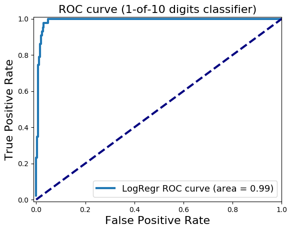
1.10b Precision-Recall, ROC curves & AUC- Python code
For Python Logistic Regression is used to plot Precision Recall, ROC curve and compute AUC
import numpy as np
import pandas as pd
import matplotlib.pyplot as plt
from sklearn.model_selection import train_test_split
from sklearn.linear_model import LogisticRegression
from sklearn.datasets import load_digits
from sklearn.metrics import precision_recall_curve
from sklearn.metrics import roc_curve, auc
#Load the digits
dataset = load_digits()
X, y = dataset.data, dataset.target
#Create 2 classes -i) Digit 1 (from digit 1) ii) Digit 0 (from all other digits)
# Make a copy of the target
z= y.copy()
# Replace all non 1's as 0
z[z != 1] = 0

X_train, X_test, y_train, y_test = train_test_split(X, z, random_state=0)
# Fit a LR model
lr = LogisticRegression().fit(X_train, y_train)

#Compute the decision scores
y_scores_lr = lr.fit(X_train, y_train).decision_function(X_test)
y_score_list = list(zip(y_test[0:20], y_scores_lr[0:20]))

#Show the decision_function scores for first 20 instances
y_score_list

precision, recall, thresholds = precision_recall_curve(y_test, y_scores_lr)
closest_zero = np.argmin(np.abs(thresholds))
closest_zero_p = precision[closest_zero]
closest_zero_r = recall[closest_zero]
#Plot
plt.figure()
plt.xlim([0.0, 1.01])
plt.ylim([0.0, 1.01])
plt.plot(precision, recall, label='Precision-Recall Curve')
plt.plot(closest_zero_p, closest_zero_r, 'o', markersize = 12, fillstyle = 'none', c='r', mew=3)
plt.xlabel('Precision', fontsize=16)
plt.ylabel('Recall', fontsize=16)
plt.axes().set_aspect('equal')
plt.savefig('fig5.png', bbox_inches='tight')

#Compute and plot the ROC
y_score_lr = lr.fit(X_train, y_train).decision_function(X_test)
fpr_lr, tpr_lr, _ = roc_curve(y_test, y_score_lr)
roc_auc_lr = auc(fpr_lr, tpr_lr)

plt.figure()
plt.xlim([-0.01, 1.00])
plt.ylim([-0.01, 1.01])
plt.plot(fpr_lr, tpr_lr, lw=3, label='LogRegr ROC curve (area = {:0.2f})'.format(roc_auc_lr))
plt.xlabel('False Positive Rate', fontsize=16)
plt.ylabel('True Positive Rate', fontsize=16)
plt.title('ROC curve (1-of-10 digits classifier)', fontsize=16)
plt.legend(loc='lower right', fontsize=13)
plt.plot([0, 1], [0, 1], color='navy', lw=3, linestyle='--')
plt.axes()
plt.savefig('fig6.png', bbox_inches='tight')
output

output
1.10c Precision-Recall, ROC curves & AUC- Python code
In the code below classification probabilities are used to compute and plot precision-recall, roc and AUC
import numpy as np
import pandas as pd
import matplotlib.pyplot as plt
from sklearn.model_selection import train_test_split
from sklearn.datasets import load_digits
from sklearn.svm import LinearSVC
from sklearn.calibration import CalibratedClassifierCV

dataset = load_digits()
X, y = dataset.data, dataset.target
# Make a copy of the target
z= y.copy()
# Replace all non 1's as 0
z[z != 1] = 0


X_train, X_test, y_train, y_test = train_test_split(X, z, random_state=0)
svm = LinearSVC()
# Need to use CalibratedClassifierSVC to redict probabilities for lInearSVC
clf = CalibratedClassifierCV(svm)
clf.fit(X_train, y_train)
y_proba_lr = clf.predict_proba(X_test)
from sklearn.metrics import precision_recall_curve

precision, recall, thresholds = precision_recall_curve(y_test, y_proba_lr[:,1])
closest_zero = np.argmin(np.abs(thresholds))
closest_zero_p = precision[closest_zero]
closest_zero_r = recall[closest_zero]
#plt.figure(figsize=(15,15),dpi=80)
plt.figure()
plt.xlim([0.0, 1.01])
plt.ylim([0.0, 1.01])
plt.plot(precision, recall, label='Precision-Recall Curve')
plt.plot(closest_zero_p, closest_zero_r, 'o', markersize = 12, fillstyle = 'none', c='r', mew=3)
plt.xlabel('Precision', fontsize=16)
plt.ylabel('Recall', fontsize=16)
plt.axes().set_aspect('equal')
plt.savefig('fig7.png', bbox_inches='tight')
output

1. Statistical Learning, Prof Trevor Hastie & Prof Robert Tibesherani, Online Stanford
2. Applied Machine Learning in Python Prof Kevyn-Collin Thomson, University Of Michigan, Coursera
Conclusion
This 4th part looked at SVMs with linear and radial basis, decision trees, precision-recall tradeoff, ROC curves and AUC.
Stick around for further updates. I’ll be back!
Comments, suggestions and correction are welcome.
Also see
1. A primer on Qubits, Quantum gates and Quantum Operations
2. Dabbling with Wiener filter using OpenCV
3. The mind of a programmer
4. Sea shells on the seashore
5. yorkr pads up for the Twenty20s: Part 1- Analyzing team”s match performance
To see all posts see Index of posts

 ML models have to be searched. This can be shown as follows
 ways to choose single feature ML models among ‘n’ features,
  ways to choose 2 feature models among ‘n’ models and so on, or


 models to search amongst in Best Fit. For 10 features this is
  or ~1000 models and for 40 features this becomes
  which almost 1 trillion. Usually there are datasets with 1000 or maybe even 100000 features and Best fit becomes computationally infeasible.
 models


 which is of the order of
  . Though forward fit is a sub optimal solution it is far more computationally efficient than best fit


 , for e.g., the inclusion of which results in the worst performance in adj Rsquared, or minimum Cp, BIC or some such criteria. At every step 1 feature is dopped. There is no guarantee that the final list of features chosen will be the best among the lot. The computation required for this is of


 to
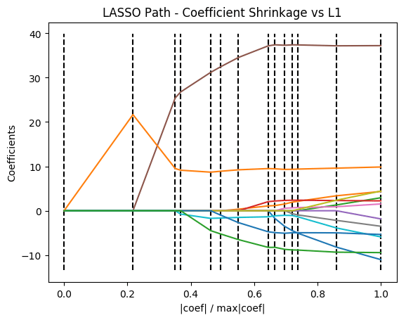
to  significantly shrinks the coefficients. We can draw a vertical line from the x-axis and read the values of the 13 coefficients. Some of them will be close to zero


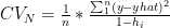
 or K choose 1, there will be K such partitions. The K Fold Cross


 is the number of elements in partition ‘K’ and N is the total number of elements

 is the diagonal hat matrix


 Then felt I like some watcher of the skies