R incantations for the uninitiated

Here are some basic R incantations that will get you started with R

A) Scalars & Vectors:
Chant 1 – Now repeat after me, with your right hand forward at shoulder height “In R there are no scalars. There are only vectors of length 1”.
Just kidding:-)

To create an integer variable x with a value 5 we write
x <- 5 or
x = 5

While the former notation may seem odd, it is actually more logical considering that the RHS is assigned to LHS. Anyway both seem to work
Vectors can be created as follows
a <- c( 2:10)
b <- c("This", "is", 'R","language")

B) Sequences:
There are several ways of creating sequences of numbers which you intend to use for your computation
<- seq(5:25) # Sequence from 5 to 25

Other ways to create sequences
Increment by 2
> seq(5, 25, by=2)
[1]  5  7  9 11 13 15 17 19 21 23 25

>seq(5,25,length=18) # Create sequence from 5 to 25 with a total length of 18
[1]  5.000000  6.176471  7.352941  8.529412  9.705882 10.882353 12.058824 13.235294
[9] 14.411765 15.588235 16.764706 17.941176 19.117647 20.294118 21.470588 22.647059
[17] 23.823529 25.000000

C) Conditions and loops
An if-else if-else construct goes like this
if(condition) {
do something
} else if (condition) {
do something
} else {
do something
}

Note: Make sure the statements appear as above with the else if and else appearing on the same line as the closing braces, otherwise R complains about ‘unexpected else’ in else statement

D) Loops
I would like to mention 2 ways of doing ‘for’ loops  in R.
a) for (i in 1:10) {
statement
}

> a <- seq(5,25,length=10)
> a
[1]  5.000000  7.222222  9.444444 11.666667 13.888889 16.111111 18.333333
[8] 20.555556 22.777778 25.000000

b) Sequence along the vector sequence. Note: This is useful as we don’t have to know  the length of the vector/sequence
for (i in seq_along(a)){
+   print(a[i])
+ }

[1] 5
[1] 7.222222
[1] 9.444444
[1] 11.66667

There are others ways of looping with ‘while’ and ‘repeat’ which I have not included in this post.

R makes manipulation of matrices and data frames really easy. All the elements in a matrix are numeric while data frames can have different types for each of the element

E) Matrix
> rnorm(12,5,2)
[1] 2.699961 3.160208 5.087478 3.969129 3.317840 4.551565 2.585758 2.397780
[9] 5.297535 6.574757 7.468268 2.440835

a) Create a vector of 12 random numbers with a mean of 5 and SD of 2
> a <-rnorm(12,5,2)
b) Convert the vector to a matrix with 4 rows and 3 columns
> mat <- matrix(a,4,3)
> mat[,1]     [,2]     [,3]
[1,] 5.197010 3.839281 9.022818
[2,] 4.053590 5.321399 5.587495
[3,] 4.225763 4.873768 6.648151
[4,] 4.709784 4.129093 2.575523

c) Subset rows 1 & 2 from the matrix
> mat[1:2,]
[,1]     [,2]     [,3]
[1,] 5.19701 3.839281 9.022818
[2,] 4.05359 5.321399 5.587495

d) Subset matrix a rows 1& 2 and with columns 2 & 3
> mat[1:2,2:3]
[,1]     [,2]
[1,] 3.839281 9.022818
[2,] 5.321399 5.587495

e) Subset matrix a for all row elements for the column 3
> mat[,3]
[1] 9.022818 5.587495 6.648151 2.575523

e) Add row names and column names for the matrix as follows
> names <- c(“tim”,”pat”,”joe”,”jim”)
> v <- data.frame(names,mat)
> v
names       X1       X2       X3
1   tim 5.197010 3.839281 9.022818
2   pat 4.053590 5.321399 5.587495
3   joe 4.225763 4.873768 6.648151
4   jim 4.709784 4.129093 2.575523

> colnames(v) <- c("names","a","b","c")
> v
names        a        b        c
1   tim 5.197010 3.839281 9.022818
2   pat 4.053590 5.321399 5.587495
3   joe 4.225763 4.873768 6.648151
4   jim 4.709784 4.129093 2.575523

F) Data Frames
In R data frames are the most important method to manipulate large amounts of data. One can read data in .csv format into data frame using
df <- read.csv(“mydata.csv”)
To get a feel of data frames it is useful to play around with the numerous data sets that are available with the installation of R
To check the available dataframes do
>data()
AirPassengers                    Monthly Airline Passenger Numbers 1949-1960
BJsales                          Sales Data with Leading Indicator
BJsales.lead (BJsales)           Sales Data with Leading Indicator
BOD                              Biochemical Oxygen Demand
CO2                              Carbon Dioxide Uptake in Grass Plants
ChickWeight                      Weight versus age of chicks on different diets
...

I will be using the mtcars data frame. Here are some of the most important commands on data frames
a) load data from mtcars
data(mtcars)
b) > head(mtcars,3) # Display the top 3 rows of the data frame
mpg cyl disp  hp drat    wt  qsec vs am gear carb
Mazda RX4     21.0   6  160 110 3.90 2.620 16.46  0  1    4    4
Mazda RX4 Wag 21.0   6  160 110 3.90 2.875 17.02  0  1    4    4
Datsun 710    22.8   4  108  93 3.85 2.320 18.61  1  1    4    1

c) > tail(mtcars,4) # Display the boittom 4 rows of the data frame
mpg cyl disp  hp drat   wt qsec vs am gear carb
Ford Pantera L 15.8   8  351 264 4.22 3.17 14.5  0  1    5    4
Ferrari Dino   19.7   6  145 175 3.62 2.77 15.5  0  1    5    6
Maserati Bora  15.0   8  301 335 3.54 3.57 14.6  0  1    5    8
Volvo 142E     21.4   4  121 109 4.11 2.78 18.6  1  1    4    2

d) > names(mtcars)  # Display the names of the columns of the data frame
[1] "mpg"  "cyl"  "disp" "hp"   "drat" "wt"   "qsec" "vs"   "am"   "gear" "carb"

e) > summary(mtcars) # Display the summary of the data frame
mpg             cyl             disp             hp             drat             wt
Min.   :10.40   Min.   :4.000   Min.   : 71.1   Min.   : 52.0   Min.   :2.760   Min.   :1.513
1st Qu.:15.43   1st Qu.:4.000   1st Qu.:120.8   1st Qu.: 96.5   1st Qu.:3.080   1st Qu.:2.581
Median :19.20   Median :6.000   Median :196.3   Median :123.0   Median :3.695   Median :3.325
Mean   :20.09   Mean   :6.188   Mean   :230.7   Mean   :146.7   Mean   :3.597   Mean   :3.217
3rd Qu.:22.80   3rd Qu.:8.000   3rd Qu.:326.0   3rd Qu.:180.0   3rd Qu.:3.920   3rd Qu.:3.610
Max.   :33.90   Max.   :8.000   Max.   :472.0   Max.   :335.0   Max.   :4.930   Max.   :5.424
qsec             vs               am              gear            carb
Min.   :14.50   Min.   :0.0000   Min.   :0.0000   Min.   :3.000   Min.   :1.000
1st Qu.:16.89   1st Qu.:0.0000   1st Qu.:0.0000   1st Qu.:3.000   1st Qu.:2.000
Median :17.71   Median :0.0000   Median :0.0000   Median :4.000   Median :2.000
Mean   :17.85   Mean   :0.4375   Mean   :0.4062   Mean   :3.688   Mean   :2.812
3rd Qu.:18.90   3rd Qu.:1.0000   3rd Qu.:1.0000   3rd Qu.:4.000   3rd Qu.:4.000
Max.   :22.90   Max.   :1.0000   Max.   :1.0000   Max.   :5.000   Max.   :8.000

f) > str(mtcars) # Generate a concise description of the data frame - values in each column, factors
'data.frame':   32 obs. of  11 variables:
$ mpg : num  21 21 22.8 21.4 18.7 18.1 14.3 24.4 22.8 19.2 ...
$ cyl : num  6 6 4 6 8 6 8 4 4 6 ...
$ disp: num  160 160 108 258 360 ...
$ hp  : num  110 110 93 110 175 105 245 62 95 123 ...
$ drat: num  3.9 3.9 3.85 3.08 3.15 2.76 3.21 3.69 3.92 3.92 ...
$ wt  : num  2.62 2.88 2.32 3.21 3.44 ...
$ qsec: num  16.5 17 18.6 19.4 17 ...
$ vs  : num  0 0 1 1 0 1 0 1 1 1 ...
$ am  : num  1 1 1 0 0 0 0 0 0 0 ...
$ gear: num  4 4 4 3 3 3 3 4 4 4 ...
$ carb: num  4 4 1 1 2 1 4 2 2 4 ...

g) > mtcars[mtcars$mpg == 10.4,] #Select all rows in mtcars where the mpg column has a value 10.4
mpg cyl disp  hp drat    wt  qsec vs am gear carb
Cadillac Fleetwood  10.4   8  472 205 2.93 5.250 17.98  0  0    3    4
Lincoln Continental 10.4   8  460 215 3.00 5.424 17.82  0  0    3    4

h) > mtcars[(mtcars$mpg >20) & (mtcars$mpg <24),] # Select all rows in mtcars where the mpg > 20 and mpg < 24
mpg cyl  disp  hp drat    wt  qsec vs am gear carb
Mazda RX4      21.0   6 160.0 110 3.90 2.620 16.46  0  1    4    4
Mazda RX4 Wag  21.0   6 160.0 110 3.90 2.875 17.02  0  1    4    4
Datsun 710     22.8   4 108.0  93 3.85 2.320 18.61  1  1    4    1
Hornet 4 Drive 21.4   6 258.0 110 3.08 3.215 19.44  1  0    3    1
Merc 230       22.8   4 140.8  95 3.92 3.150 22.90  1  0    4    2
Toyota Corona  21.5   4 120.1  97 3.70 2.465 20.01  1  0    3    1
Volvo 142E     21.4   4 121.0 109 4.11 2.780 18.60  1  1    4    2

i) > myset <- mtcars[(mtcars$cyl == 6) | (mtcars$cyl == 4),] # Get all calls which are either 4 or 6 cylinder
> myset
mpg cyl  disp  hp drat    wt  qsec vs am gear carb
Mazda RX4      21.0   6 160.0 110 3.90 2.620 16.46  0  1    4    4
Mazda RX4 Wag  21.0   6 160.0 110 3.90 2.875 17.02  0  1    4    4
Datsun 710     22.8   4 108.0  93 3.85 2.320 18.61  1  1    4    1
Hornet 4 Drive 21.4   6 258.0 110 3.08 3.215 19.44  1  0    3    1
Valiant        18.1   6 225.0 105 2.76 3.460 20.22  1  0    3    1
Merc 240D      24.4   4 146.7  62 3.69 3.190 20.00  1  0    4    2…

j) > mean(myset$mpg) # Determine the mean of the set created above
[1] 23.97222

k) > table(mtcars$cyl) #Create a table of cars which have 4,6, or 8 cylinders

4  6  8
11  7 14

G) lapply,sapply,tapply
I use the iris data set for these commands
a) > data(iris) #Load iris data set

b) > names(iris)  #Show the column names of the data set
[1] "Sepal.Length" "Sepal.Width"  "Petal.Length" "Petal.Width"  "Species"
c) > lapply(iris,class) #Show the class of all the columns in iris
$Sepal.Length
[1] "numeric"
$Sepal.Width
[1] "numeric"
$Petal.Length
[1] "numeric"
$Petal.Width
[1] "numeric"
$Species
[1] "factor"

d) > sapply(iris,class) # Display a summary of the class of the iris data set
Sepal.Length  Sepal.Width Petal.Length  Petal.Width      Species
"numeric"    "numeric"    "numeric"    "numeric"     "factor"

e) tapply: Instead of getting the mean for each of the species as below we can use tapply
> a <-iris[iris$Species == "setosa",]
> mean(a$Sepal.Length)
[1] 5.006
> b <-iris[iris$Species == "versicolor",]
> mean(b$Sepal.Length)
[1] 5.936
> c <-iris[iris$Species == "virginica",]
> mean(c$Sepal.Length)
[1] 6.588

> tapply(iris$Sepal.Length,iris$Species,mean)
setosa versicolor  virginica
5.006      5.936      6.588

Hopefully this highly condensed version of R will set you on a R-oll.

You may like
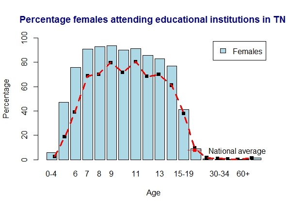
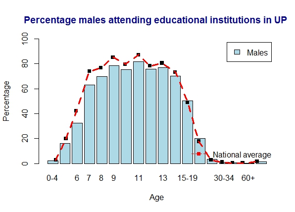
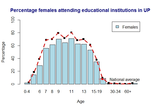
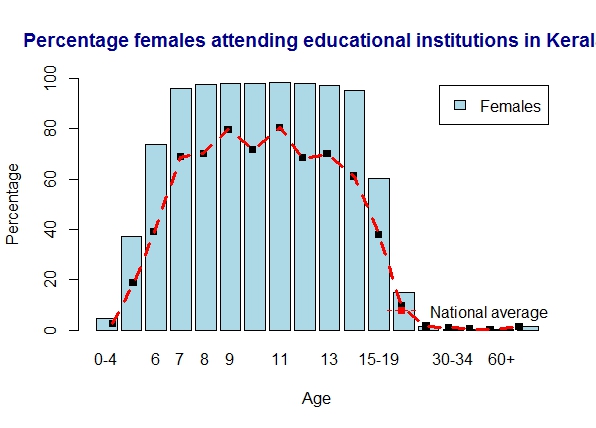
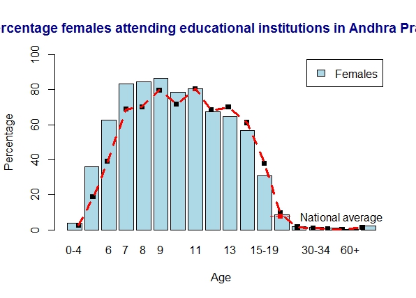
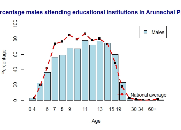
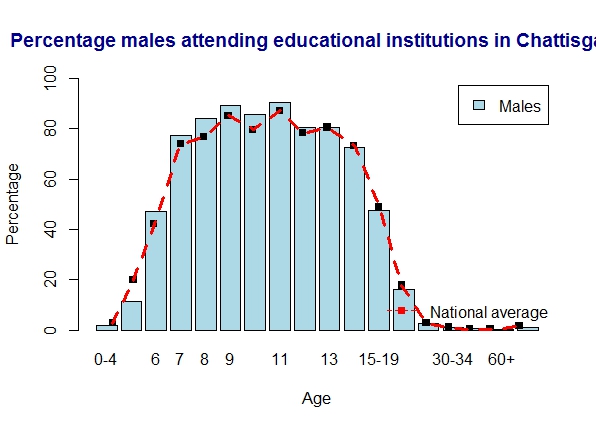
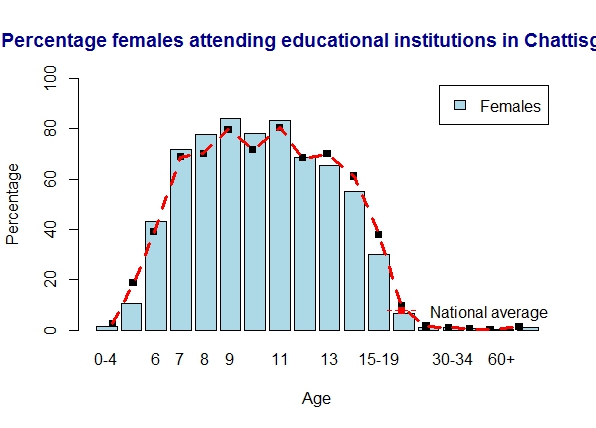
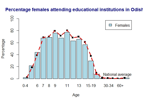
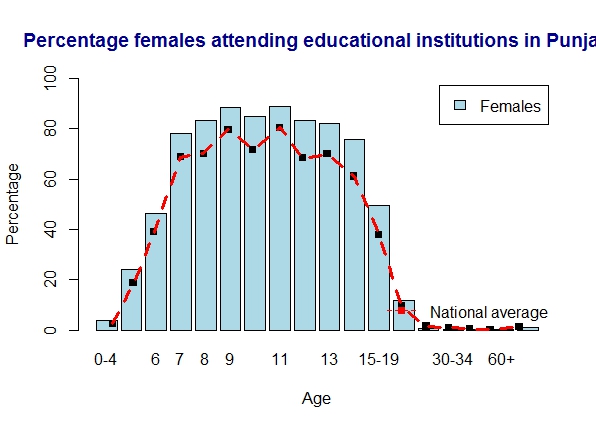
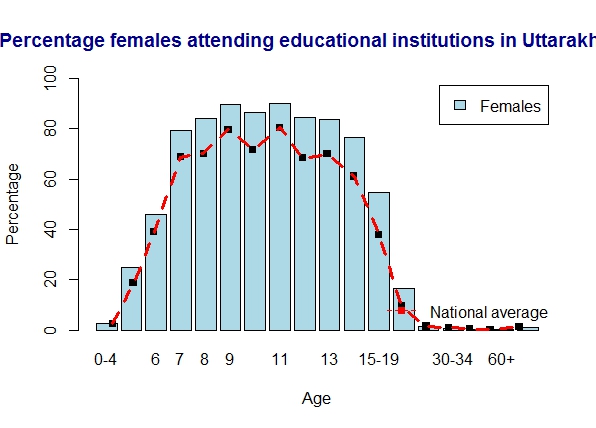
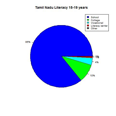
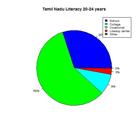
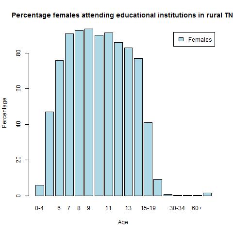
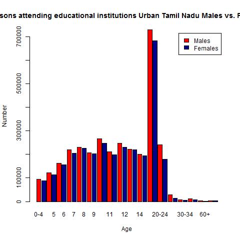
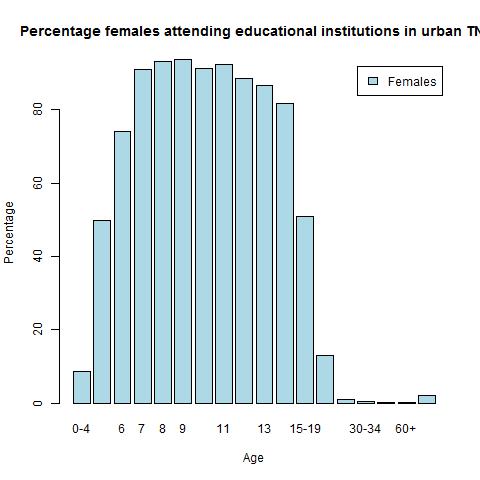
– A peek into literacy in India:Statistical learning with R
– A crime map of India in R: Crimes against women
– Analyzing cricket’s batting legends – Through the mirage with R

Programming Zen and now – Some essential tips-2

This post is a follow-up to my earlier post – How to program – Some essential tips. In this post I expand on some of the ideas of my earlier post.

Programming means different things to different people. To some programming is a drudgery almost akin to manual labor, to others programming is an insurmountable mountain full of frustrations and disappointments while to others it is an intense problem solving and a creative activity. In my opinion programming can mean anything to you. It is your attitude towards coding that make it a chore, a daunting task or something really creative.

Here are some my insights on how to go about learning to code

Eyes wide open:  People generally get frustrated when a piece of code that they wrote does not do what they intended it to do. In some cases the code snippet will do nothing when they were expecting final result, sometimes the code will crash or it will go into an infinite loop and drive the person nuts. (Let me assure you – I have been there, done that!) The usual reaction when this happens is anger and frustration where we generally tinker around with the code only to get the same result. Soon the emotions will progress from anger to hopelessness.

The first thing that one needs to while coding is to keep your ‘eyes wide open’. We tend to be  guilty of ignoring the error messages that show up. Here one way to attack coding

a) Fully understand the ‘what’ of the problem. If there is an infinite loop or a core dump check after which point does it happen? If there is an execution error, what is the error trying to tell us?
b) Next look into ‘why’  the error occurred.  You could either use debugger or insert appropriate print statements to take the offending code apart.
c) Thirdly think ‘how‘ you can address the situation. Make appropriate changes and re-run the code
d) Did it solve the issue.If yes, move forward. Otherwise go to step a)

Remember that we learn more from our programming mistakes more than when our code just ‘happens’ to work!  Mistakes in our code make us to explain every part of the program

Changing times:

Times have changed. Programming Zen and programming now are worlds apart. In many ways, IDEs, Git, Google etc. have made the programmer’s life a lot easier

‘Git’ing from here to there:  Here is a trick that I learnt fairly recently, though it should have occurred to me more than 2 years back. This is using Git judiciously for all programming tasks (Note:  I am saying nothing new here!).  I find it really useful in writing code with incremental changes.  I create my initial code on the master and then test out incremental changes on a ‘new branch’ even for personal projects. Once I have proved a small increment works, I merge it with the ‘main’ branch. I again start working on the ‘new’ for the next incremental change followed by a merge to the master

The steps are

Make initial changes

1. git add  .
2. git commit –m “ Initial changes’

Create a new branch
3. git checkout –b ‘new

Make incremental changes. Test.
4.git add  .
5. git commit –m “Change 1”

Merge with the master
6.git checkout master
7. git merge new

Continue to work with ‘new’.
8 . git checkout new
9. Go to step 4)

This process can be continued till you get your final product. I find this extremely useful instead of just using an IDE to make code changes. Invariably you can run into a situation where you had something working some time back and in the next instant it is broken and you can’t figure out all the changes you made to the working code. This can be extremely frustrating. With Git you have a history of changes and you can switch to an earlier version of working code and start from there.

Rarely do I find a reason to have more than 1 branch

Here is a pictorial version of this

1

Taking help from Dr. Google: For most questions and errors that you encounter you will find others who have hit similar bugs. Just google it. You will more than surprised that others went down the exact same path that you are treading.  Besides the internet is full of tutorials, blogs and articles on key aspects of programming

Explore the cave of Stack overflow:   Spend time exploring Stack overflow. Stack overflow is replete with code snippets and questions that you wanted to ask. There is so much information out there. If you really don’t find an answer to your problem, post it in Stack overflow and you are bound to get an answer or a link to a similar question asked previously

Finally programming requires dollops of patience. Develop patience along with your skill in coding and soon programming will much more enjoyable to you.

1. Programming languages in layman’s language
2. The common alphabet of programming languages
3. How to program – Some essential tips
4. The mind of a programmer

You may also like
1. A crime map of India in R: Crimes against women
2.  What’s up Watson? Using IBM Watson’s QAAPI with Bluemix, NodeExpress – Part 1
3.  Bend it like Bluemix, MongoDB with autoscaling – Part 2
4. Informed choices through Machine Learning : Analyzing Kohli, Tendulkar and Dravid
5. Thinking Web Scale (TWS-3): Map-Reduce – Bring compute to data
6. Deblurring with OpenCV:Weiner filter reloaded

A crime map of India in R – Crimes against women

In this post I take a look at the gory crime scene across India to determine which states are the heavy weights in crimes. Who is the undisputed champion of rapes in a year? Which state excels in cruelty by husbands and the relatives to wives? Which state leads in dowry deaths? To get the answers to these questions I perform analysis of the state-wise crime data against women with the data  from Open Government Data (OGD) Platform India. The dataset  for this analysis was taken for the Crime against Women from OGD.

(Do see my post Revisiting crimes against women in India which includes an interactive Shiny app)

The data in OGD is available for crimes against women in different states under different ‘crime heads’ like rape, dowry deaths, kidnapping & abduction etc. The data is available for years from 2001 to 2012. This data is plotted as a scatter plot and a linear regression line is then fit on the available data. Based on this linear model,  the projected incidence of crimes likes rapes, dowry deaths, abduction & kidnapping is performed for each of the states. This is then used to build a table of  different crime heads for all the states predicting the number of crimes till the year 2018. Fortunately, R  crunches through the data sets quite easily. The overall projections of crimes against as women is shown below based on the linear regression for each of these states

Projections over the next couple of years
The tables below are based on the projected incidence of crimes under various categories assuming that these states maintain their torrid crime rate. A cursory look at the tables below clearly indicate the Uttar Pradesh is the undisputed heavy weight champion in 4 of 5 categories shown. Maharashtra and Andhra Pradesh take 2nd and 3rd ranks in the total crimes against women and are significant contenders in other categories too.

A) Projected rapes in India
The top 3 heavy weights in projected rapes over the next 5 years are 1) Madhya Pradesh  2) Uttar Pradesh 3) Maharashtra

rapes

Full table: Rape.csv
B) Projected Dowry deaths in India 
dowrydeaths

Full table: Dowry Deaths.csv
C) Kidnapping & Abduction
kidnapping

Full table: Kidnapping&Abduction.csv
D) Cruelty by husband & relatives
cruelty

Full table: Cruelty by husbands_relatives.csv
E) Total crimes against women

total

Full table: Total crimes.csv
Here is a visualization of ‘Total crimes against women’  created as a choropleth map

1The implementation for this analysis was done using the  R language.  The R code, dataset, output and the crime charts can be accessed at GitHub at crime-against-women

Directory structure
– R code
dataset used
output
statewise-crime-charts

The analysis has been completely parametrized. A quick look at the implementation is shown  below. A function state crime was created as given below

statecrime.R
This function (statecrime.R)  does the following
a) Creates a scatter plot for the state for the crime head
b) Computes a best linear regression fir and draws this line
c) Uses the model parameters (coefficients) to compute the projected crime in the years to come
d) Writes the projected values to a text file
c) Creates a directory with the name of the state if it does not exist and stores the jpeg of the plot there.

statecrime <- function(indiacrime, row, state,crime) {
year <- c(2001:2012)
# Make seperate folders for each state
if(!file.exists(state)) {
dir.create(state)
}
setwd(state)
crimeplot <- paste(crime,".jpg")
jpeg(crimeplot)

# Plot the details of the crime
plot(year,thecrime ,pch= 15, col="red", xlab = "Year", ylab= crime, main = atitle,
,xlim=c(2001,2018),ylim=c(ymin,ymax), axes=FALSE)

A linear regression line is fit using ‘lm’

# Fit a linear regression model
lmfit <-lm(thecrime~year)
# Draw the lmfit line
abline(lmfit)

The model parameters are then used to draw the line and also project for the next 5 years from 2013 to 2018

nyears <-c(2013:2018)
nthecrime <- rep(0,length(nyears))
# Projected crime incidents from 2013 to 2018 using a linear regression model
for (i in seq_along(nyears)) {
nthecrime[i] <- lmfit$coefficients[2] * nyears[i] + lmfit$coefficients[1]
}

The projected data for each state is appended into an appropriate file which is then used to display the tables at the top of this post

# Write the projected crime rate in a file
nthecrime <- round(nthecrime,2)
nthecrime <- c(state, nthecrime, "\n")
print(nthecrime)
#write(nthecrime,file=fileconn, ncolumns=9, append=TRUE,sep="\t")
filename <- paste(crime,".txt")
# Write the output in the ./output directory
setwd("./output")
cat(nthecrime, file=filename, sep=",",append=TRUE)

The above function is then repeatedly called for each state for the different crime heads. (Note: It is possible to check the read both the states and crime heads with R and perform the computation repeatedly. However, I have done this the manual way!)

crimereport.R
# 1. Andhra Pradesh
i <- 1
statecrime(indiacrime, i, "Andhra Pradesh","Rape")
i <- i+38
statecrime(indiacrime, i, "Andhra Pradesh","Kidnapping& Abduction")
i <- i+38
statecrime(indiacrime, i, "Andhra Pradesh","Dowry Deaths")
i <- i+38
statecrime(indiacrime, i, "Andhra Pradesh","Assault on Women")
i <- i+38
statecrime(indiacrime, i, "Andhra Pradesh","Insult to modesty")
i <- i+38
statecrime(indiacrime, i, "Andhra Pradesh","Cruelty by husband_relatives")
i <- i+38
statecrime(indiacrime, i, "Andhra Pradesh","Imporation of girls from foreign country")
i <- i+38
statecrime(indiacrime, i, "Andhra Pradesh","Immoral traffic act")
i <- i+38
statecrime(indiacrime, i, "Andhra Pradesh","Dowry prohibition act")
i <- i+38
statecrime(indiacrime, i, "Andhra Pradesh","Indecent representation of Women Act")
i <- i+38
statecrime(indiacrime, i, "Andhra Pradesh","Commission of Sati Act")
i <- i+38
statecrime(indiacrime, i, "Andhra Pradesh","Total crimes against women")
...
...

and so on for all the states

Charts for different crimes against women

1) Uttar Pradesh

The plots for  Uttar Pradesh  are shown below

Rapes in UP

Rape

Dowry deaths in UP

Dowry Deaths

Cruelty by husband/relative

Cruelty by husband_relatives

Total crimes against women in Uttar Pradesh

Total crimes against women

You can find more charts in GitHub by clicking Uttar Pradesh

2) Maharashtra : Some of the charts for Maharashtra

Rape

Rape

Kidnapping & Abduction

Kidnapping& Abduction

Total crimes against women in Maharashtra

Total crimes against women

More crime charts  for Maharashtra

Crime charts can be accessed for the following states from GitHub ( in alphabetical order)

3) Andhra Pradesh
4) Arunachal Pradesh
5) Assam
6) Bihar
7) Chattisgarh
8) Delhi (Added as an exception based on its notoriety)
9) Goa
10) Gujarat
11) Haryana
12) Himachal Pradesh
13) Jammu & Kashmir
14) Jharkhand
15) Karnataka
16) Kerala
17) Madhya Pradesh
18) Manipur
19) Meghalaya
20) Mizoram
21) Nagaland
22) Odisha
23) Punjab
24) Rajasthan
25) Sikkim
26) Tamil Nadu
27) Tripura
28) Uttarkhand
29) West Bengal

The code, dataset and the charts can be cloned/forked from GitHub at crime-against-women

Let me know if you find any interesting patterns in the data.
Thoughts, comments welcome!


See also
My book ‘Practical Machine Learning with R and Python’ on Amazon
A peek into literacy in India: Statiscal learning with R

You may also like
– Analyzing cricket’s batting legends – Through the mirage with R
– What’s up Watson? Using IBM Watson’s QAAPI with Bluemix, NodeExpress – Part 1
– Bend it like Bluemix, MongoDB with autoscaling – Part 1

A peek into literacy in India: Statistical Learning with R

In this post I take a peek into the literacy landscape across India as a whole using R language.  The dataset from Open Government Data (OGD) platform India was used for this purpose. This data is based on the 2011 census. The XL sheets for the states were downloaded for data for each state. The Union Territories were not included in the analysis.

A thin slice of the data from each data set was taken from the data for each individual state (Note: This could also have been done from the consolidated india.xls XL sheet which I came to know of, much later).

I calculate the following for age group

Males (%) attending education institutions = (Males attending educational institutions * 100)/ Total males
Females (%) attending education institutions = (Females attending educational institutions * 100)/ Total Females

This is then plotted as a bar chart with the age distribution. I then overlay the national average for each state over the barchart to check whether the literacy in the state is above or below the national average. The implementation in R is included below

The code and data can be forked/cloned from GitHub at india-literacy

The results based on the analysis is given below.

  1. Kerala is clearly the top ranker with the literacy rates for both males and females well above the average
  2. The states with above average literacy are – Kerala, Himachal Pradesh, Uttarakhand, Tamil Nadu, Haryana, Himachal Pradesh, Karnataka, Maharashtra, Punjab, Uttarakhand
  3. The states with just about average literacy – Karnataka, Andhra Pradesh, Chattisgarh, Gujarat, Madhya Pradesh, Odisha, West Bengal
  4. The states with below average literacy – Uttar Pradesh, Bihar, Jharkhand, Arunachal Pradesh, Assam, Jammu and Kashmir, Jharkhand, Rajasthan


A brief implementation of the basic code in R is shown bwelow

# Read the Arunachal Pradhesh literacy related data
arunachal = read.csv("arunachal.csv")
# Create as a matrix
arunachalmat = as.matrix(arunachal)
arunachalTotal = arunachalmat[2:19,7:28]
# Take transpose as this is necessary for plotting bar charts
arunachalmat = t(arunachalTotal)
# Set the scipen option to format the y axis (otherwise prints as e^05 etc.)
getOption("scipen")
opt <- options("scipen" = 20)
getOption("scipen")
#Create a vector of total Males & Females
arunachalTotalM = arunachalmat[3,]
arunachalTotalF = arunachalmat[4,]
#Create a vector of males & females attending education institution
arunachalM = arunachalmat[6,]
arunachalF = arunachalmat[7,]
#Calculate percent of males attending education of total
arunachalpercentM = round(as.numeric(arunachalM) *100/as.numeric(arunachalTotalM),1)
barplot(arunachalpercentM,names.arg=arunachalmat[1,],main ="Percentage males attending educational institutions in Arunachal Pradesh",
xlab = "Age", ylab= "Percentage",ylim = c(0,100), col ="lightblue", legend= c("Males"))
points(age,indiapercentM,pch=15)
lines(age,indiapercentM,col="red",pch=20,lty=2,lwd=3)
legend( x="bottomright",
legend=c("National average"),
col=c("red"), bty="n" , lwd=1, lty=c(2),
pch=c(15) )
#Calculate percent of females attending education of total
arunachalpercentF = round(as.numeric(arunachalF) *100/as.numeric(arunachalTotalF),1)
barplot(arunachalpercentF,names.arg=arunachalmat[1,],main ="Percentage females attending educational institutions in Arunachal Pradesh ",
xlab = "Age", ylab= "Percentage", ylim = c(0,100), col ="lightblue", legend= c("Females"))
points(age,indiapercentF,pch=15)
lines(age,indiapercentF,col="red",pch=20,lty=2,lwd=3)
legend( x="bottomright",
legend=c("National average"),
col=c("red"), bty="n" , lwd=1, lty=c(2),
pch=c(15) )

A) Overall plot for India

a) India – Males

india-males

b) India – females

india-females

The plots for each individual state is given below

1) Literacy in Tamil Nadu

Tamil Nadu is slightly over the national average. The women seem to do marginally better than the males

a) Tamil Nadu – males

tn-males

b) Tamil Nadu – females

tn-females

2) Literacy in Uttar Pradesh

UP is slightly below the national average. Women are comparatively below men here

a) Uttar Pradesh – males

UP-males

b) Uttar Pradesh – females

UP-females

3) Literacy in Bihar

Bihar is well below the national average for both men and women

a) Bihar – males

bihar-males

b) Bihar – females

bihar-females

4. Literacy in Kerala

Kerala is the winner all the way in literacy with almost 100% literacy across all age groups

a) Kerala – males


kerala-females

b) Kerala -females

kerala-females


5. Literacy in Andhra Pradesh

AP just meets the national average for literacy.

a) Andhra Pradesh – males

andhra-males

b) Andhra Pradesh – females

andhra-females

6. Literacy in Arunachal Pradesh

Arunachal Pradesh is below average for most of the age groups

a) Arunachal Pradesh – males

arunachal-males

b) Arunachal Pradesh – females

arunachal-females

7. Literacy in  Assam

Assam is below national average

a) Assam – males

assam-males

b) Assam – females

assam-females


8. Literacy in Chattisgarh

Chattisgarh is on par with the national average for both men and women

a) Chattisgarh – males

chattisgarh-males

b) Chattisgarh – females

chattisgarh-females


9. Literacy in Gujarat

Gujarat is just about average

a) Gujarat – males

gujarat-males

b) Gujarat – females

gujarat-females

10. Literacy in Haryana

Haryana is slightly above average

a) Haryana – males

haryana-males

b) Haryana – females

haryana-females11.  Literacy in Himachal Pradesh

Himachal Pradesh is cool and above average.

a) Himachal Pradesh – males

himachal-males


b) Himachal Pradesh – females

himachal-females

12. Literacy in Jammu and Kashmir

J & K is marginally below average

a) Jammu and Kashmir – males

jk-males

b) Jammu and Kashmir – females

jk-females


13. Literacy in Jharkhand

Jharkhand is some ways below average

a) Jharkhand – males

jharkand-males

b) Jharkhand – females

jharkand-feamles

14. Literacy in Karnataka

Karnataka is on average for men. Womem seem to do better than men here

a) Karnataka – males

karnataka-males

b) Karnataka – females

karnataka-females

15. Literacy in Madhya Pradesh

Madhya Pradesh meets the national average

a) Madhya Pradesh – males

mp-males

b) Madhya Pradesh – females

mp-females

16. Literacy in Maharashtra

Maharashtra is front-runner in literacy

a) Maharashtra – females

maharashtra

b) Maharastra – females

maharashtra-feamles


17. Literacy in Odisha

Odisha meets national average

a) Odisha – males

odisha-males

b) Odisha – females

odisha-females


18. Literacy in  Punjab

Punjab is marginally above average with women doing even better

a) Punjab – males

punjab-males

b) Punjab – females

punjab-females19. Literacy in Rajasthan

Rajasthan is average for males and below average for females

a) Rajasthan – males

rajashthan-males

b) Rajasthan – females

rajasthan-females20. Literacy in Uttarakhand

Uttarakhand rocks and is above average

a) Uttarakhand – males

uttarkhan-males

b) Uttarakhand – females

uttarkhand-females

21. Literacy in West Bengal

West Bengal just about meets the national average.

a) West Bengal – males

wb-males


b) West Bengal – females

wb-females

The code can be cloned/forked from GitHub  india-literacy. I have done my analysis on the overall data. The data is further sub-divided across districts in each state and further into urban and rural. Many different ways of analysing are possible. One method is shown here

Conclusion

  1. Kerala is clearly head and shoulders above all states when it comes to literacy
  2. Many states are above average. They are Kerala, Himachal Pradesh, Uttarakhand, Tamil Nadu, Haryana, Himachal Pradesh, Karnataka, Maharashtra, Punjab, Uttarakhand
  3. States with average literacy are – Karnataka, Andhra Pradesh, Chattisgarh, Gujarat, Madhya Pradesh, Odisha, West Bengal
  4. States which fall below the national average are – Uttar Pradesh, Bihar, Jharkhand, Arunachal Pradesh, Assam, Jammu and Kashmir, Jharkhand, Rajasthan

See also
– A crime map of India in R: Crimes against women
– What’s up Watson? Using IBM Watson’s QAAPI with Bluemix, NodeExpress – Part 1
– Bend it like Bluemix, MongoDB with autoscaling – Part 1

Statistical learning with R: A look at literacy in Tamil Nadu

In this post I make my first foray into data mining using the R language. As a start, I picked up the data from the Open Government Data (OGD Platform of India from the Ministry of Human Resources. There are many data sets under Education. To get started I picked the data set on Tamil Nadu which deals with the population attending educational institutions by age, sex and institution type. Similar data is available for all states.

I wanted to start off on a small scale, primarily to checkout some of the features of the R language. R is clearly the language of choice for processing large amounts of data. R has close to 4000+ packages that can do various things like statistical, regression analysis etc. However I found this is no easy task. There are a zillion ways in which you can take cross-sections of a large dataset. Some of them will provide useful insights while others will lead you nowhere.

Also see my post Literacy in India – A deepR dive!

Data science, which is predicted to be the technology of the future based on with the mountains of data being generated daily, will in my opinion, will be more of an art and less of a science. There will be wizards who will be able to spot remarkable truths in the mundane data while others will not be that successful.

Anyway back to my attempt to divine intelligence in the Tamil Nadu(TN)  literacy data. The data downloaded was an Excel sheet with 1767 rows and 28 columns. The first 60 rows deal with the overall statistics of literacy in Tamil Nadu state as a whole. Further below are the statistics on the individual districts of Tamil nadu.
Each of this is further divided into urban and rural parts. The data covers persons from the age of 4 upto the age of 60 and whether they attended school, college, vocational institute etc. To make my initial attempt manageable I have just focused on the data for Tamil Nadu state as a whole including the breakup of the urban and rural data.

My analysis is included below. The code and the dataset for this implementation is in R language and can be cloned from GitHub at tamilnadu-literacy-analysis

Analysis of Tamil Nadu (total)
The total population of Tamil Nadu based on an age breakup is shown below

1) Total population Tamil Nadu 
tntotal

2) Males  & Females attending education institutions in TN

tneduThere are marginally more males attending educational institutions. Also the number of persons attending educational institutions seems to drop from 11 years of age. There is a spike around 20-24 years and people go to school and college at this age. See pie chart 8) below

3) Percentage of males attending educational institution of the total males

percenteduM

4) Percentage females attending educational institutions in TN 

percenteduF

There is a very similar trend between males and females. The attendance peaks between 9 – 11 years of age and then falls to roughly 50% around 15-19 years and rapidly falls off

5) Boys and girls attending school in TN

tnschool

For some reason there is a marked increase for boys and girls around 20-24. Possibly people repeat classes around this age

6) Persons attending college in TN

tncollege

7) Educational institutions attended by persons between 15- 19 years

tnschool-1

8) Educational institutions attended by persons between 20-24 tnschool-2

As can be seen there is a large percentage (30%)  of people in the 20-24 age group who are in school. This is probably the reason for the spike in “Boys and girls attending school in TN” see 2) for the 20-24 years of age

Education in rural Tamil Nadu

1) Total rural population Tamil Nadu 

ruraltotal

2) Males  & Females attending education institutions in  rural TNruraledu3) Percentage of rural males attending educational institution

percentruralM

4) Percentage females attending educational institutions in rural TN of total females

percentruralF

The persons attending education drops rapidly to 40% between 15-19 years of age for both males and females

5) Boys and girls attending school in rural TN

ruralschool

6) Persons attending college in rural TN

ruralcollege

7) Educational institutions attended by persons between 15- 19 years in rural TN

rural-1

8) Educational institutions attended by persons between 20-24 in rural TN

rural-2

As can be seen there is a large percentage (39%)  of rural people in the 20-24 age group who are in school

Education in urban Tamil Nadu

1) Total population in urban Tamil Nadu 

urbantotal

2) Males  & Females attending education institutions in urban TNurbanedu3) Percentage of males attending educational institution of the total males in urban TNpercentruralM4) Percentage females attending educational institutions in urban TN

percenturbanF

5) Boys and girls attending school in urban TN

urbanschool

6) Persons attending college in urban TN

urbancollege

7) Educational institutions attended by persons between 15- 19 years in urban TN

urban-1

8) Educational institutions attended by persons between 20-24 in urban TN

urban-2

As can be seen there is a large percentage (25%) of rural people in the 20-24 age group who are in school

The R implementation and the Tamil Nadu dataset can be cloned from my repository in GitHub at tamilnadu-literacy-analysis 

The above analysis is just one of a million possible ways the data can be analyzed and visually represented. I hope to hone my skill as progress along in similar analysis.

Hasta la vista! I’ll be back.

Watch this space!