‘Would you tell me, please, which way I ought to go from here?’ ‘That depends a good deal on where you want to get to,’ said the Cat. ‘I don’t much care where—’ said Alice. ‘Then it doesn’t matter which way you go,’ said the Cat. ‘—so long as I get somewhere,’ Alice added as an explanation. ‘Oh, you’re sure to do that,’ said the Cat, ‘if you only walk long enough.’
Alice in Wonderland, Lewis Caroll, 1864
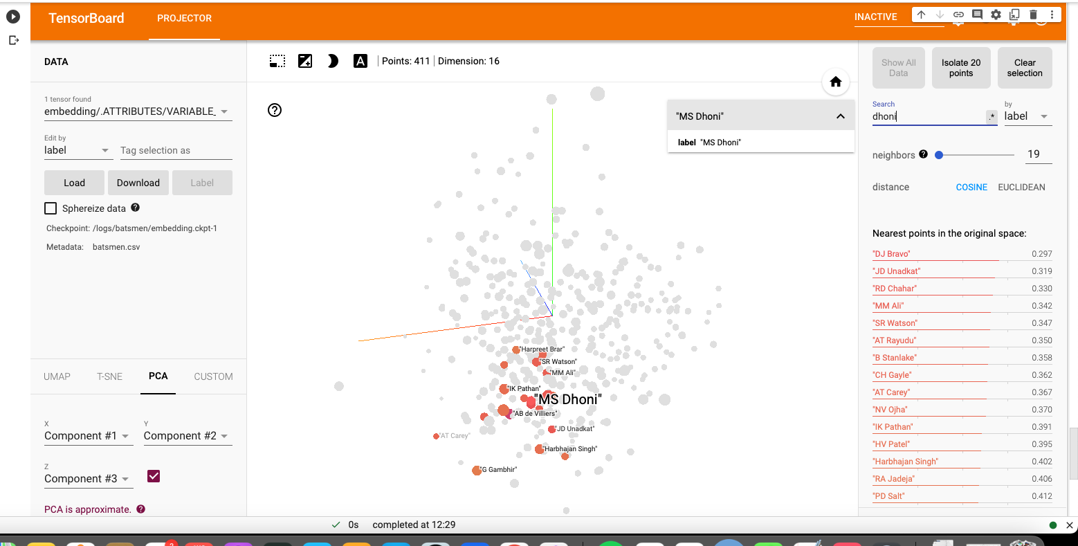
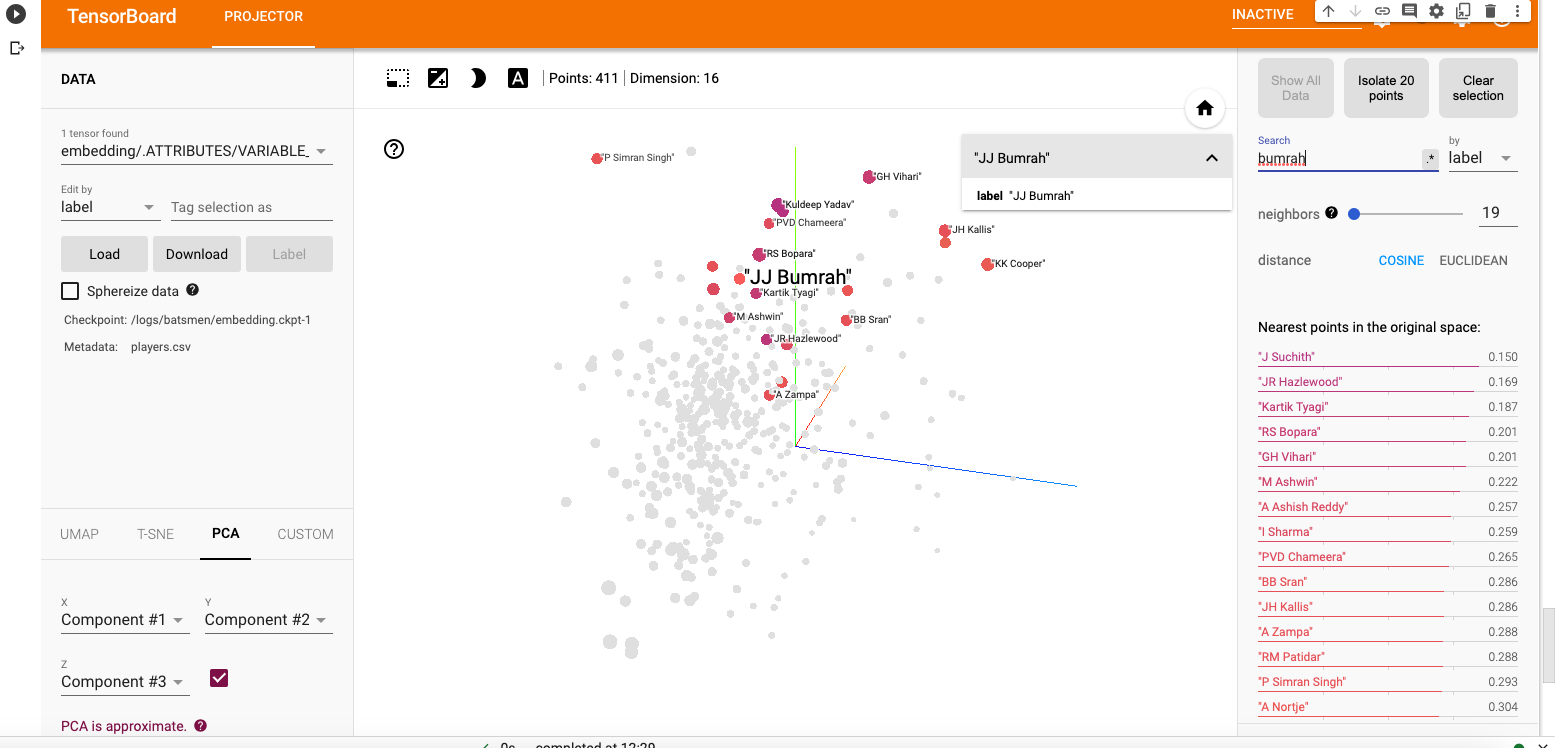
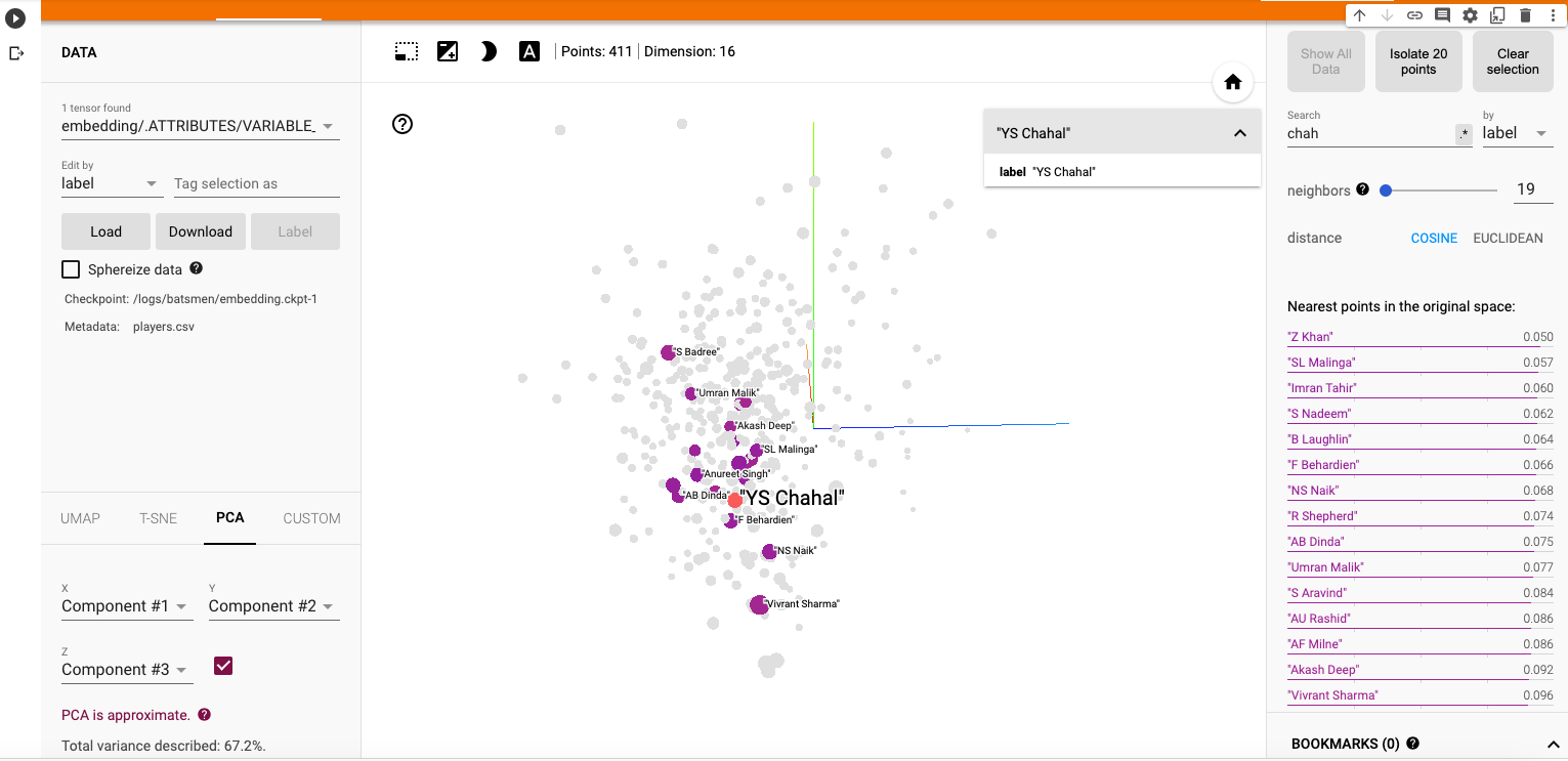
About three years ago, I implemented a T20 Match Win Probability model, using Deep Learning with batsman and bowler embeddings to compute the the ball-by-ball probability of winning by the competing teams as the match progresses (see GooglyPlusPlus: Win Probability using Deep Learning and player embeddings.). Ball-by-ball match data is available for different T20 leagues in Cricsheet. This Deep Learning algorithm was originally written in TensorFlow and Keras at that time (Win Probabilty Computation – TensorflowKeras). I had got a training and validation accuracy of around 0.8876 (this is very similar to Win Probability model in baseball, NFL etc.)
I recently, revisited this code and asked Sonnet 4.6 to convert the TensorFlow-Keras DL algorithm into PyTorch, (more compact and probably more efficient), which it promptly did, without breaking a sweat. However, even after converting to Pytorch, the validation accuracy still remained ~ 0.8959 (see notebook Match Win Probability Computation – Pytorch). The T20 Win Probability Model was trained on 2.14 million rows of T20 data taken from 9 different T20 leagues across the globe. The ball-by-ball match data is available in Cricsheet as yaml files which have been pre-processed suitably.
I was wondering whether it was possible to use Karpathy’s auto-research to optimise this DL algorithm Providentially, I came across EPOCH: An agentic protocol for multi-round system optimisation by Liu, Li, and Srikanth (2026), which was a paper that was published by my colleagues at Prorata.ai. EPOCH, enables system fine-tuning, optimisations of model, code, and rule-based components. Since, this was exactly what I wanted, I decided to give EPOCH a try. The result was quite impressive!!!
The setup and installation was pretty straightforward. I then started EPOCH by typing in /epoch in Claude Code. Initially, I was just given a set of questions. I set the goal of 0.95 as the target validation accuracy for the agentic protocol.
Incidentally, earlier, I did try a couple of things to improve the performance of the DL algorithm by playing around with the hyper-parameters, including brute-force Gridsearch, but none of it seemed to help. I think I hit a plateau around 0.8876.
EPOCH, created an initial scaffolding and baseline metrics. It then ran multiple experiments to optimise the validation accuracy which started to inch towards 0.95. Here is a summary of the experiments of EPOCH and the outcomes. EPOCH and Claude Code stored the baseline metrics and results of each experiment in github repo claude_wpa
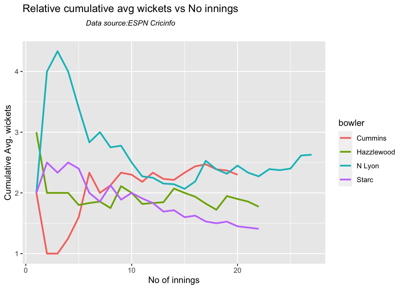
a) Hyperparameter tuning vsValidation accuracy improvement
Included below are the hyperparameter changes and the corresponding validation accuracy improvement in each round
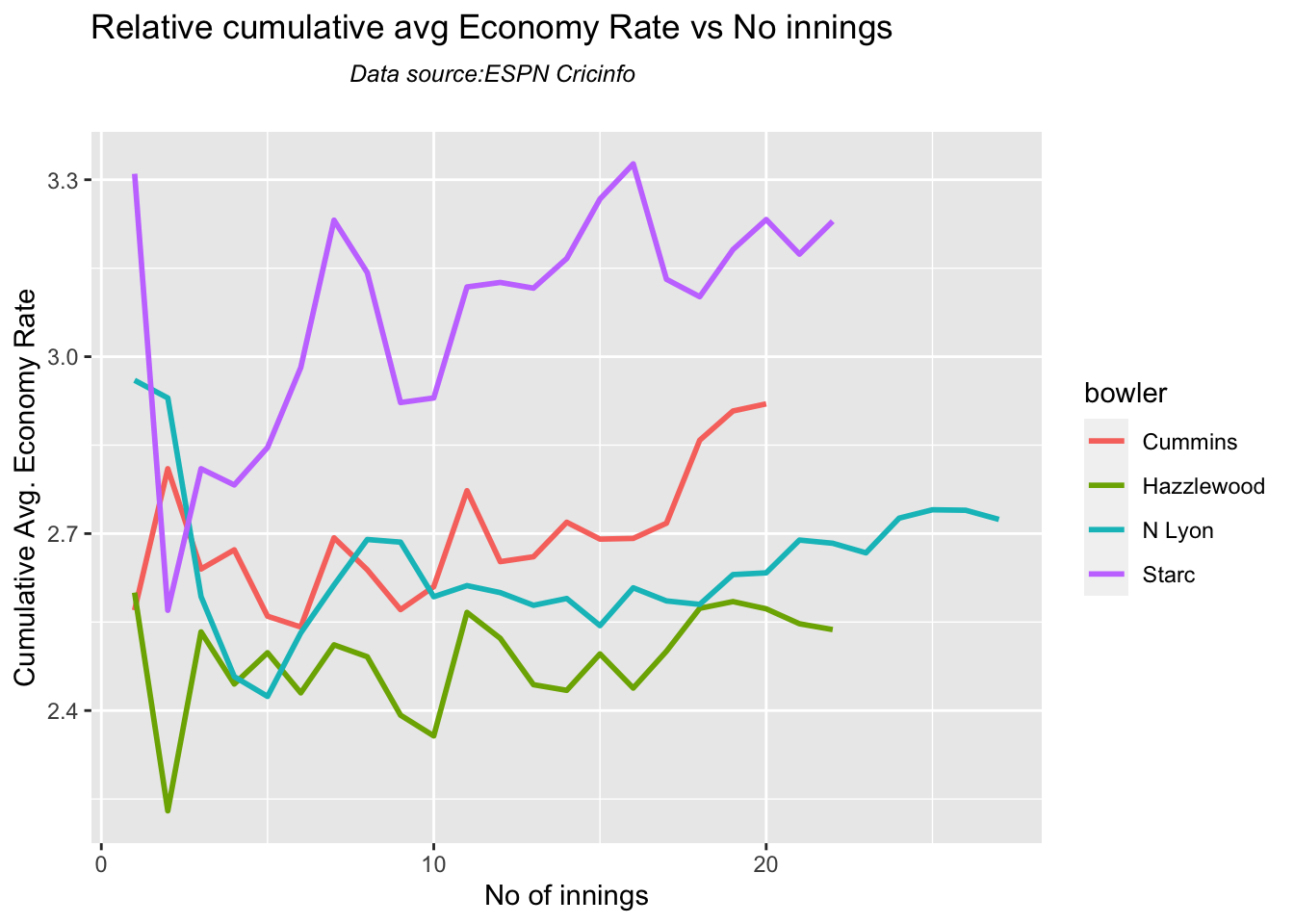
b) Train vs Validation Accuracy improvement in final round
EPOCH Optimization — Experiment Log
#
Change Made
Val Acc
Delta
Verdict
Remarks
1
Baseline: emb=16, ep=20, lr=0.01
0.8876
—
Baseline
Starting point. 16-dim embeddings for 7,785 batsmen + 5,742 bowlers is severely under-capacity.
2
epochs: 20 → 40 (emb=16)
0.8937
+0.0061
❌ REJECT
More epochs alone not enough — embedding bottleneck is the real constraint.
3
emb: 16 → 32, epochs=40
0.9157
+0.0281
✅ ACCEPT
Biggest single jump (+2.81%). Doubling embedding capacity gave the model enough room to represent player identities.
4
emb: 32 → 64, epochs=40
0.9297
+0.0140
✅ ACCEPT
Scaling embedding further yielded another solid gain. Diminishing returns beginning to show.
5
emb: 64 → 128, epochs=80, lr=0.01
0.9369
+0.0072
✅ ACCEPT
Good gain. LR scheduler fired at ep76 with only 4 epochs left — couldn’t fully exploit the reduction.
6
epochs: 80 → 100 (emb=128)
0.9419
+0.0050
❌ REJECT
2nd LR drop just starting at ep95–100 when training ended. Model plateaued at 0.9419.
7
epochs: 100 → 150 (emb=128)
0.9450
+0.0081
❌ REJECT
Progress, but just below the min_delta threshold. 3rd LR drop just beginning.
8
epochs: 150 → 200 (emb=128)
0.9452
+0.0083
✅ ACCEPT
3rd LR scheduler drop fully exploited. Well-regularized (train_eval_gap = −0.0017). Final model.
Key Findings
Finding
Detail
Embedding dim was the biggest lever
Going 16→32→64→128 drove most of the accuracy gain (+4.93% combined)
LR scheduler is crucial but fires late
ReduceLROnPlateau (patience=3, factor=0.5) fires at ~ep71, ~ep110, ~ep155 — each firing gives ~+0.005
Epochs must be long enough post-firing
Each LR drop needs ~40–50 epochs to propagate — that’s why ep=200 was needed
No overfitting throughout
train_eval_gap was always small and negative (−0.0017 to −0.0061), meaning BatchNorm+Dropout regularized well
lr=0.001 from random init causes regression
Tried lower LR early on — model under-converged. lr=0.01 with scheduler is the right combination
Total improvement: 0.8876 → 0.9452 (+6.76%) across 8 experiments.
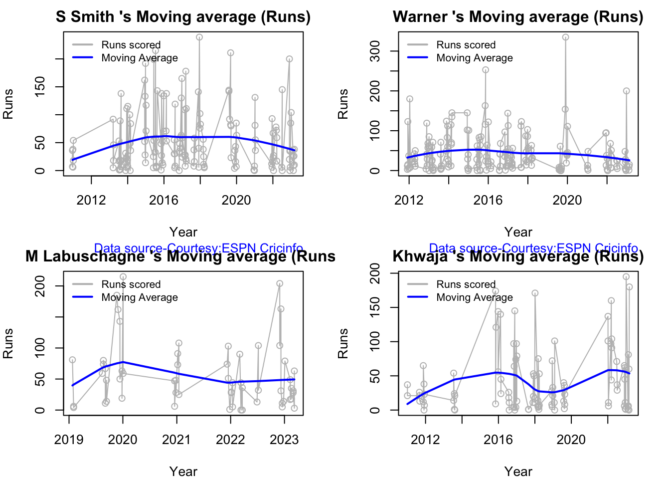
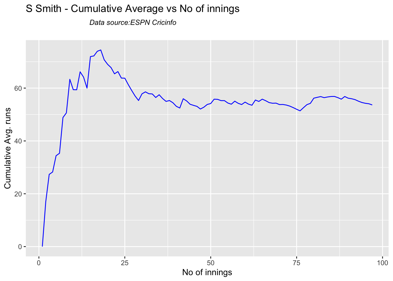
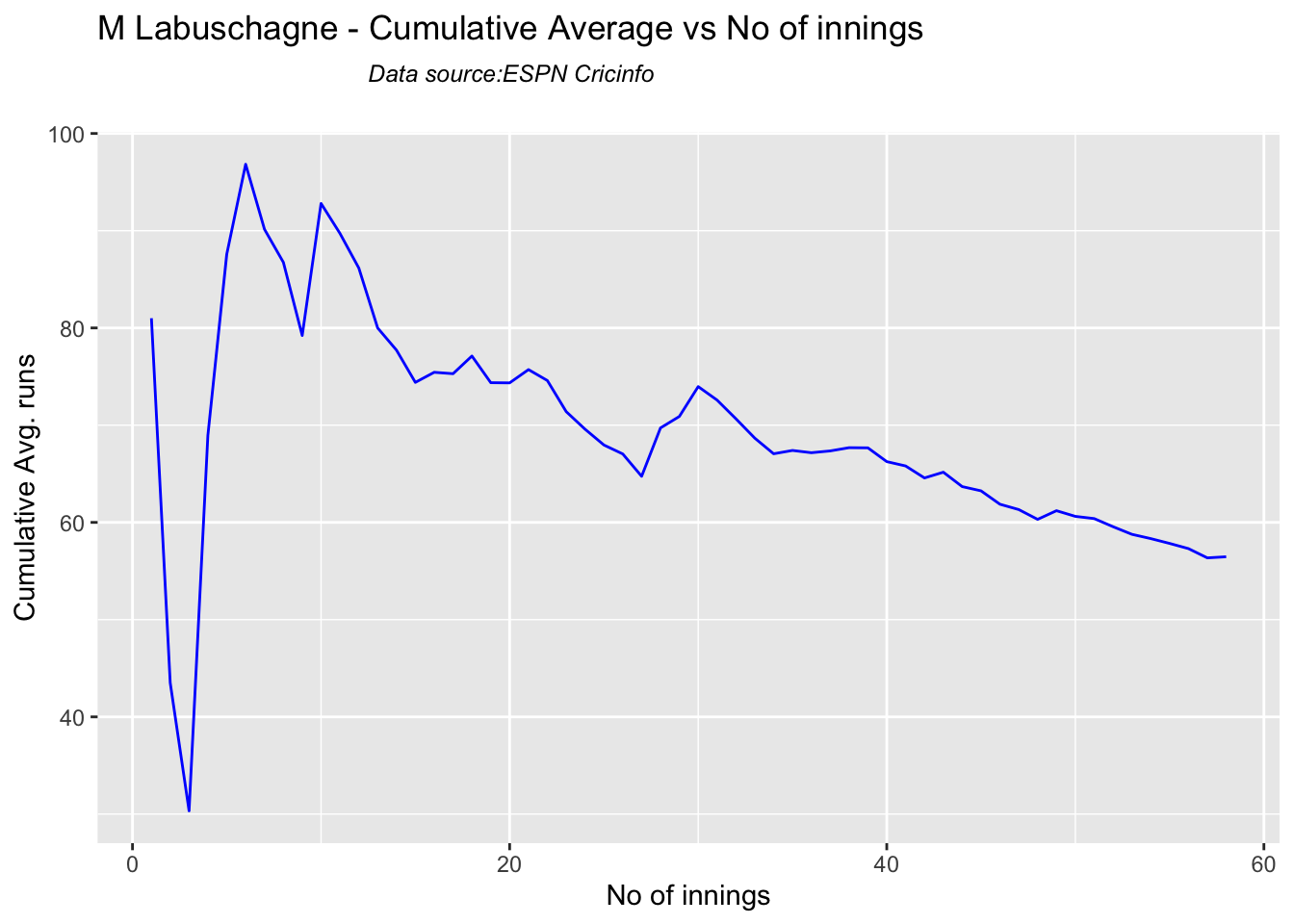
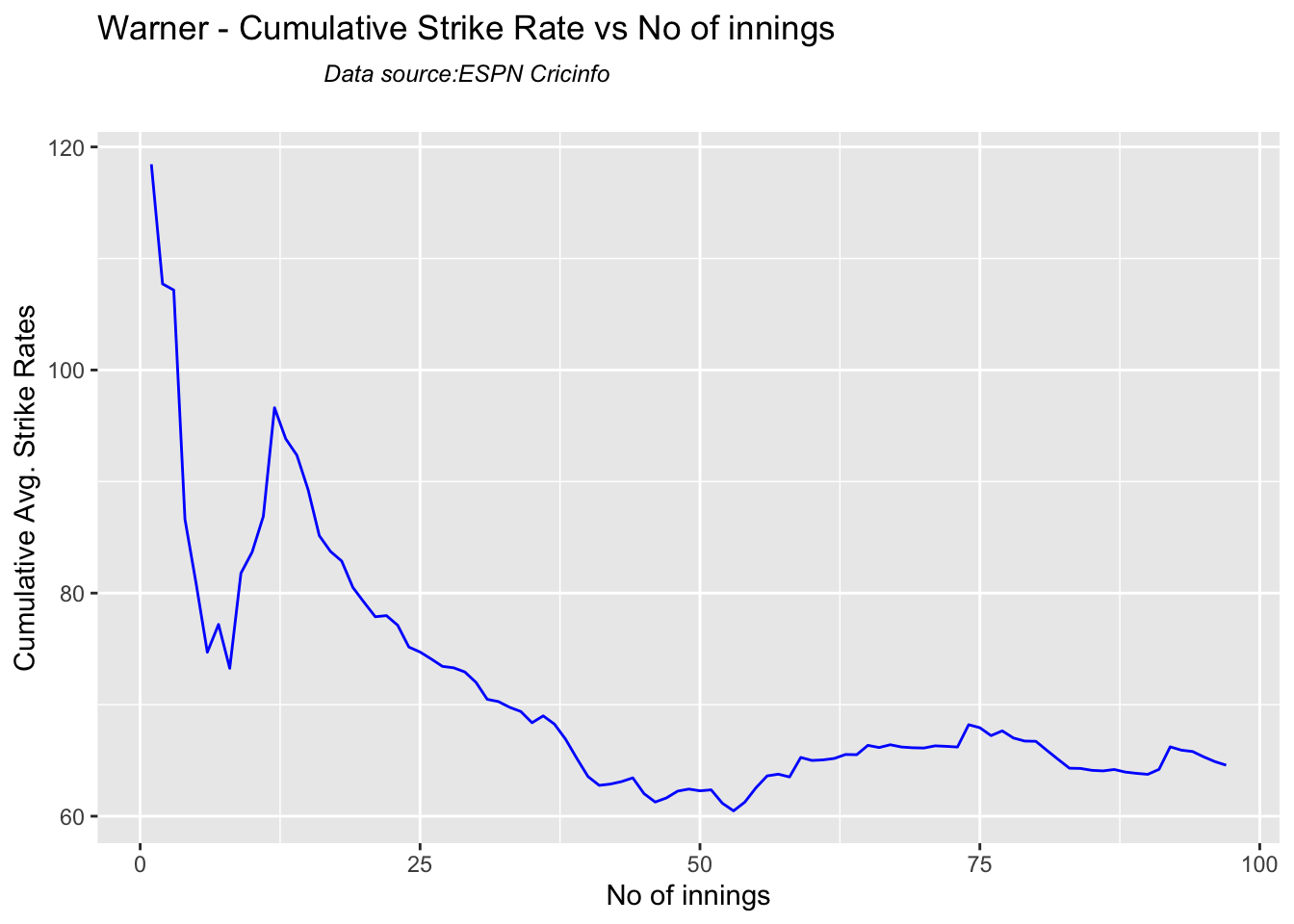
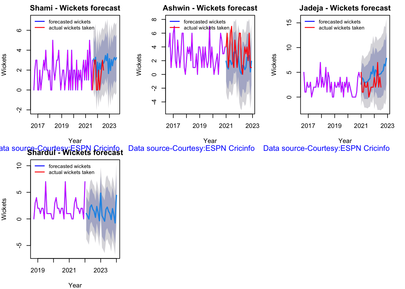
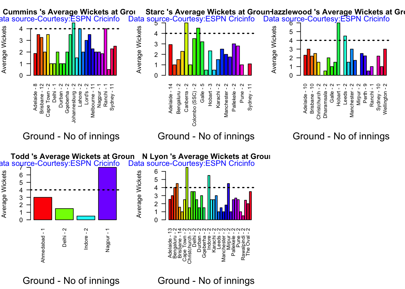
The final trained T20 Win Probability model had a validation accuracy of 0.9452 at which point I stoppd further experiments. This model was downloaded with all the necessary metadata which included the trained weights, the architecture config, and the standard scaler, which needs to be applied on any new data on which the model is actually applied. The trained T20 Win Probability DL Model was applied the three T20 matches in the latest ICC T20 World Cup held this year from Feb 07,206 to Mar 8, 2026.
The ball-by-ball Win probability for each team in the T20 match is computed in the charts below. There will be two charts for each of the matches.
a) Win Probability- Side-by-side chart : The first chart is a side-by-side Win Probability Analysis where the win probability of each team will be computed using the DL model on a ball-by-ball basis. The win probability of the other team is just 100 minus the win probability of the first team.
b) Win Probability – Overlapping chart : This chart will be computed using the Deep Learning model for each team independently on a ball-by-ball basis, and then both the probabilities will be super-imposed on one another so that we can see how the probability changed and whether the second team, which had to chase a total, actually was able to do so. If it could, then the win probability would actually exceed the the first team with Win Probability
I will be taking the final three matches of this ICC World Cup in 2026 namely to use the Win Proability Model against
1) West Indies vs India – Quarter Finals – Winner – India (1 Mar 2026)
In this this match, Sanju Samson stood like a rock and played a well-paced innings and chased the target comfortably scoring 97 runs not out.
a) Side-by-side chart
b) Overlapping chart
2) India vs England – Semi Finals – Winner- India (5 Mar 2026)
India set a sizable target of 253 with good contributions from Sanju Samsom, Shivam Dube and Ishan Kishan
a) Side-by-side chart
b) Overlapping chart
3) India vs New Zealand – Finals – Winner – India (8 Mar 2026)
Put into bat first, India put up a mammoth total of 255 with contributions from Sanju Samson, Abhishek Sharma, Ishan Kishan, and Shivam Dube. New Zealand lost wickets regularly and could not keep up with the required run rate, which kept climbing ever so high, so it was never in contention
a) Side-by-side chart
b) Overlapping chart
Conclusion
It was quite interesting to see agentic protocol EPOCH work. Things have really changed these days, with the agents automatically making judgement calls on what would be hyper-parameter changes would result in better performance. I remember I had used Grid Search to optimise the DeepLearning algorithm, but it didn’t help much.
Tomorrow and tomorrow and tomorrow Creeps in this petty pace from day to day To the last syllable of recorded time, And all our yesterdays have lighted fools The way to dusty death. Out, out, brief candle!
Life’s but a walking shadow, a poor player That struts and frets his hour upon the stage And then is heard no more. It is a tale Told by an idiot, full of sound and fury, Signifying nothing.
Macbeth, Act V, Scene Vby William Shakespeare
The IPL 2026 carnival is just around the corner, and my enhanced IPL app “IPL AI Oracle” is just in time for IPL fans. The current version of IPL AI Oracle, refines my earlier implementation to be more accurate and to handle a wider range of natural language queries related to IPL. My previous post “Introducing IPL AI Oracle: AI that speaks cricket!!! discusses an implementation which had 4 tabs
General queries
Match Analysis
Head-to-head
Team vs All Teams
The data for this app comes from Cricsheet. The data consists of ball-by-ball data for all IPL matches since 2006 in yaml format. This data was then pre-processed into a suitable format for use by the tabs both for the analytics and the natural language query functionality
The tabs provide analytics of IPL matches, head-to-head and team vs All Teams. Each of the 4 tabs allow for user query in natural language based on the tab general queries, queries on IPL matches, queries on head-to-head performance between 2 teams and natural language queries between a team versus All Teams.
For details about the implementation, please see the post “Introducing IPL AI Oracle: AI that speaks cricket!!! The IPL analytics are based on my Python package ‘yorkpy‘. which itself is based on its earlier avatar ‘yorkr‘ in R available in CRAN. For handling the natural language queries, in my previous implementaion, I used prompt templates for each of the tabs which would construct an appropriate prompt to gpt-4.1-nano LLM. Ths earlier implementation with prompt templates worked fine for a reasonable number of user queries. However, for each user query the prompt constructed was quite large and guzzled up tokens quite fast and I was running out of my subscription very early.
So, in this current implementation I finetune gpt-4o-mini-2024-07-18, one of the smaller gpt models, to keep the costs low. The prompt templates were reduced to the bare minimum. The gpt-40-mini-2024-17-18 model is then trained on hand-created individual training examples for each tab. The initial set of training examples was around 220 queries with corresponding pandas code. The split is as follows
matches: 65 rows
head_to_head: 50 rows
teamVsAllTeams: 48 rows
general_queries: 39 rows
This is the ground truth from which all other examples were created. Subsequently, I used Claude Sonnet 4.5 to augment the initial set of questions. The amplification essentially consisted of different ways of asking the same query for example
What is V Kohli’s strike rate in IPL?
Show me V Kohli’s strike rate
V Kohli’s strike rate
Display V Kohli’s strike rate etc
Can you tell me V Kohli’s Strike rate
Find V Kohli’s Strike rate
…
The augmented data set was used in finetuning. The finetuning process was done several times as I would take each finetuned model and test it manually. I would find issues. Sometimes the question pattern itself would be missing or it would generate incorrect response Fortunately Sonnet 4.5 helped me to identify patterns which were under-represented or were inconsistent with other queries with similar patterns. Additional training examples were added for complex queries which required the generation of a lot of code for e.g. the batting or bowling scorecard in matches, head_to_head or teamAllTeams
The original training examples are augmented to produce 2760 examples with 12 variations for simple patterns and 15 training examples for complex ones. The scorecard code is further boosted and the final number of training examples are 3831 training data which cannbe split into
matches: 1212 examples
head_to_head: 1032 examples
teamVsAllTeams: 1002 examples
general_queries: 585 examples
This training data is then shuffled and split into training and validation in the ratio of 3447 (90%) : 384 (10%).
The base model was gpt-4o-mini-2024-07-18 which was the smallest and most economical. The default hyper parameters were used
Epochs – 3
Batch size – 6
LR multiplier – 1.8
Seed – 3
Train loss – 0.000
Validation loss – 0.003
Full validation loss – 0.002
Try out the enhanced IPL AI Oracle – https://wizard-ai-three.vercel.app/ (When you click the above link, a page will open. Enter your email and click ‘Send magic link‘ button below. This will send a magic link to your email. Click the ‘Sign in’ button which will allow you login to the app IPL AI Oracle and start using it.)
Natural language queries
Here are some random natural language queries in different tabs
A) General queries tab
This tab deals with general on IPL queries
1) Top 3 scorers in IPL 2025?
…
2) What is Virat Kohli’s best years in IPL?
3) How many ducks did Rohit Sharma score in IPL?
4) What is Ravindra Jadeja’s Economy rate?
B) Matches tab
This tab deals with a selected individual match
Batting scorecard of CSK
2) How many runs did RR score in powerplay?
3) Who were the top 3 bowlers in this match?
4) Who took wickets for in middle overs for Delhi Capitals?
C) Head to head tab
This tab takes into consideration all matches played between the 2 selected teams
Bowling scorecard of Delhi Capitals
2. Who took the most wickers for KKR?
3) Who were the top scorers for KKR in death overs?
D) Team vs All Teams
Who were most wicket takers for Chennai Super Kings in death over?
2. How many sixes did Dhoni hit in death overs?
3. Which batsmen from Gujarat Titans scored more than 100 runs?
In addition I have added 2 other tabs to the earlier tabs. Now there is
Batting Analysis tab
Bowling Analysis tab
These tab provide various batting and bowling analytics for IPL players
IPL AI Oracle can make mistakes and sometimes generate erroneous code
If the answer is wrong try to rephrase the question.
Try to use the full name Rohit Sharma if possible
You can use abbreviations like ER, SR and for teams CSK, RCB, KKR etc
IPL AI Oracle is not always one shot, sometimes it is 2-shot
I will try to improve the model in future versions. For the current version I had to do some of the steps including the testing manually. I would like to experiment with Claude Code and automate the generation of training data, finetuning, testing using the finetuned model (using a test harness) and subsequently correcting/adding to the training data if needed repeating the steps again till the tests pass with a high degree of accuracy. Lets see.
A puzzling behaviour of subatomic particles, like photons or electrons, is that when they are sent through two narrow slits, they create an interference pattern on the detection screen, just as waves do. This suggests that each particle behaves like a wave of probability, passing through both slits simultaneously. However, the moment you try to observe or detect which slit the particle goes through, the interference pattern disappears. The particle no longer behaves like a wave. Instead, it acts like a discrete particle, choosing one slit or the other as though it had never been a wave at all. The conclusion: “observation collapses the wave-like nature into particle-like reality”.
“If you can explain this using common sense and logic, do let me know, because there is a Nobel Prize for you.” — Prof. Jim Al-Khalili
Do watch this utterly engaging presentation on the double-slit experiment by Prof. Jim Al-Khalili (Double Slit Experiment explained! by Jim Al-Khalili)
When the Wave Remembered …
This is a short science fiction inspired by the bizarre behaviour of sub atomic particleslike photons, electrons etc.
– The Slits Between Worlds
Dr. Mira Sen had spent her life staring at a pair of slits cut into a sheet of carbon black metal.
To others they were just part of a physics experiment, an echo of the century-old setup that revealed the dual nature of light. But Mira believed they were far more. She believed the slits were a doorway.
And tonight, she would prove it.
For years, high precision photon detectors sat beside the slits, ready to observe the incoming light. Every time the detectors were active, the photons behaved like particles, solid, singular, predictable. But when she powered the detectors off, something impossible happened: the interference pattern changed slightly each time, as if influenced by something other than her instruments.
Something aware.
– Awareness Creates Reality
Human consciousness, Mira theorized, was not trapped in the flesh. It was the observation center of a far more expansive self, one that existed across countless universes, overlapping like waves until the moment we focused on one.
“Your body,” she wrote once, “is simply the particle-form collapse of a much larger wave-self.”
Tonight she chose to test that idea.
– The Turning Off
She shut off the detectors.
The lab grew silent, no clicks, no readouts, no hum of machinery. Only the low vibration of the laser remained, like a distant temple bell.
For the first time in years, Mira allowed herself to stop analyzing, stop measuring, stop controlling. She sat on the floor beside the apparatus and closed her eyes.
She slowed her breath. One inhale. One exhale. Another inhale, followed by an exhale. A simple presence, pure being, thoughtless and open. Tranquility. Silence. A stillness that felt timeless.
It was the kind of stillness she had tasted only during meditation retreats in the Himalayas, a state the monks called satori, a moment of sudden seeing.
In that quiet, something shifted inside her, a subtle widening of awareness, a soft dissolving of the boundary between observer and observed.
The world outside faded. The world within opened.
And in that inner silence, something responded.
The pattern on the wall brightened, not by the mechanics of the experiment, but as though an intelligence woven through probability itself was leaning toward her awareness.
A voice formed, not from the air, but inside her mind. We are you.
– The Wave-Selves
Her knees weakened. “You mean, versions of me?”
Versions, extensions, variations. You collapse into matter only here. Across most realities you are wave form, unbounded, and aware.
“But why reveal yourselves now?” she asked.
Because you finally stopped watching long enough for us to show you.
A chill passed through her. All her life she had been observing, measuring, controlling. But the wave selves existed only when unobserved, free of the restrictions of attention.
It was not the detectors that collapsed the wave. It was consciousness itself.
Human existence in physical form was simply an accident of focus.
The Shutter of the Mind
“What am I supposed to do?” Mira asked.
The shifting pattern grew brighter.
Remember.
– The Flash of Ancient Knowledge
At that word, something ancient stirred in her.
Suddenly she recalled what Indian mystics had whispered through the ages: behind the individual atman lies the infinite Brahman, pure consciousness, the ocean from which all selves arise. In Hindu philosophy it is mentioned as “Tat tvam asi” or “Thou art that!”
The truth resonated like a struck gong. She was not merely Mira. She was a ripple of Brahman temporarily collapsed into form.
Then came another flash, this time of Buddhism she had studied in college. The Four Stages of Nirvana from the Sutta Pitaka cascaded through her awareness:
Stream Enterer, the first glimpse beyond illusion
Once Returner, one foot in the world and one in the infinite
No Returner, dissolving the boundary
Arahant, the one fully freed
The levels were not steps on a ladder, she realized. They were states of collapse and un-collapse, stages of releasing the illusion of particle-self to awaken the wave-self.
As she felt her multiversal versions overlapping, she understood: mysticism and physics were describing the same doorway, one through observation, the other through liberation.
And now she was crossing it.
A shutter in her mind lifted. Suddenly she felt herself stretch into dimensions she had no words for, countless Mira selves overlapping, harmonising, existing as probability, as potential, as pure presence.
Her body dissolved like sand in water.
But she did not vanish.
She expanded.
For an eternal moment, she knew herself as a wave across universes, a being of consciousness, not flesh, a presence that shaped reality by attention alone.
– Collapse
Her assistant Jonas arrived late, saw the detectors turned off, and frowned. “Dr. Sen? Did you leave in a hurry?”
He flipped the detectors on.
The interference pattern snapped back to normal.
And on the floor beside the machine, he found her lab coat, but not Mira.
She had collapsed into a different reality the moment he observed the experiment again.
Somewhere across the multiversal ocean, wave Mira rippled outward and smiled.
She was free at last…
Author’s note:As mentioned at the top, this story draws inspiration from the puzzling behavior of photons and electrons. Although I first learned about the double-slit experiment in my college days, I never fully appreciated its significance until recently. I had been toying with this theme for a few days and had a few key ideas, but I found it difficult to weave them into a coherent narrative. Then an idea struck me. I have been using AI-assisted coding for about a year — why not explore AI’s help in the creative process as well? With the assistance of ChatGPT 5.1, I was able to flesh out the story. Just as in coding, I still had to nudge, correct, refine, and fix logical flaws along the way. The first image was generated with Gemini’s Nano Banana and the second image with GPT-4o. The theme, direction, and final narrative choices are entirely my own.I am quite pleased with the result.
What would you think if I sang out of tune? Would you stand up and walk out on me? Lend me your ears and I’ll sing you a song And I’ll try not to sing out of key
Oh, I get by with a little help from AI Mm, I get high with a little help from AI Mm, gonna try with a little help with AI
Adapted from “With A Little Help From My Friends” from the album Sgt. Pepper’s Lonely Heart Club Band, Beatles, 1967
Introduction For quite some time I have been wanting to create an application that allows user to query cricket data in plain English (Natural Language Query) and get the appropriate answer. Finally, I have been able to realise this idea with my latest application “IPL AI Oracle:AI that speaks cricket!!!“. While I have just done this for IPL, it can be done for any of the other T20 leagues namely (Intl. T20 Men’s and Women’s, BBL, PSL, NTB, CPL, WBBL etc.). The current app “IPL AI Oracle” is in Python, and is a distant cousin of my Shiny app GooglyPlusPlus written entirely in R (see IPL 2023:GooglyPlusPlus now with by AI/ML models, near real-time analytics!)
GooglyPlusPlus is much more sophisticated with detailed analytics of batsmen, bowlers, teams, matches, head-to-head, team-vs-AllTeams, batsmen and bowler ranking and analyis. GooglyPlus also includes ball-by-ball Win Probability models using Logistic Regression and Deep Learning models. While, ‘IPL AI Oracle’ lacks the ML/DL models it includes the ability to answer user queries in simple English (Natural Language Query -NLQ) and generate the pandas code for the same.
IPL AI Oracle
The IPL AI Oracle has a 2 main modules
frontend
backend
a) Frontend
The frontend is made with Next.js, Typescript and has 4 tabs
General queries
Match Analysis
Head-to-head
Team vs All Teams
The frontend includes analytics for matches, head-to-head and team-vs-allTeams options. Plots can be generated for some features and uses Plotly.js for rendering of plots
b) Backend
The backend implements FastAPI endpoints for the different analytics and natural language queries. A) The analytics in the 3 tabs namely match analysis, head-to-head and team vs All teams are implemented using my Python package ‘yorkpy‘. Since my package yorkpy has all the cricket rules baked into it, I used the code from my package verbatim for these tabs.
B) The data for the analytics comes from Cricsheet. Cricsheet includes ball-by-ball data in yaml, for all IPL matches from the beginning of time. This data is pre-processed with R utilities of my Shiny app GooglyPlusPlus. These R functions to convert the match data into the data required format for the a) Match Analysis Tab b) Head-to-head tab and c) Team vs All Teams tab which are then subsequently converted to csv for use by my package yorkpy. My Python package is based on pandas and can process this data and display the analytics required for the tabs
C) Plotly is used for generating the plots
D) Jinja templates are used for creating the prompts for the different tabs
D) For natural language query in each tab, originally I used Ollama and tried out Mistral 7Band DeepSeek Coder 6.7B. But then I realised that it has a large footprint, if deployed, and hence settled for gpt-4.1-nano
The frontend is deployed on Vercel and the backend is dockerised and deployed on Railway. Since the clock is ticking for Vercel, Railway and GPT API, I will be closely monitoring the usage.
Give IPL AI Oracle a try. Click this link IPL AI Oracle. (When you click the link you will be asked to enter your email address, to which a magic link will be sent. Clicking the link will give access to the link. Please wait 2-3 minutes for the mail, if still not received check your spam/trash folder)
Here are some random screenshots from the different tabs
I) IPL Analytics A) Match Analysis a) Batting scorecard – Chennai Super Kings vs Gujarat Titans (2025-05-25)
b) Batsmen vs Bowlers (Mumbai Indians vs Delhi Capitals – 2025-04-13)
B) Head-to-head Analysis
a) Top Bowlers Performance (Delhi Capitals vs Kolkata Knight Riders – all matches) This tab takes into consideration all matches played between these 2 teams and computes analytics between these 2 teams
b) Wicket Types Analysis (Rajasthan Royals vs Mumbai Indians – all matches)
C) Team vs All Teams
a) Team Bowling Scorecard – Royal Challengers Bangalore
II) Natural Language Query (User queries)
A) General Queries i) How many runs did V Kohli score in total ?
ii) How runs did MS Dhoni score in 2017?
iii) Which team won the most matches?
iv) Which bowler has the best economy rate?
v) How many times did Chennai Super Kings defeat Rajasthan Royals?
vi) How many wickets did Bumrah take in 2017?
B) Match analysis – Natural Language query
To use the Natural Language Query in this tab, you have to choose the match. For e.g.Chennai Super Kings vs Mumbai Indians (2025-04-20). Selecting a match between 2 teams will automatically create natural language chips (with red arrow). You can select any one of the chips (button) or type in your own question and click Ask Question
i) Who scored the most runs in this match?
This can be verified by selecting the Batting scorecard for the match
ii) Who took the most wickets in this match?
iii) What is the economy rate of JC Archer?
C) Head-vs-Head (Natural Language Query)
Before typing in a Natural Language Query (NLQ) ensure that Team 1 and Team 2 are selected
a) Which bowler took the most wickets between Royal Challengers Bangalore and Chennai Super Kings?
b) Which batsmen scored between 30 to 40 runs in these matches?
D) Team vs All Teams (Natural Language Query)
Remember to select the Team before using NLQ
a) Who are the top 3 batsman for Gujarat Titans?
b) What was Punjab King’s win percentage?
How I Built IPL AI Oracle (with a Little Help from AI)
Here are key highlights behind the build
Data for this app comes from Cricsheet which provides ball-by-ball details in every IPL match as yaml files
Pre-processing of these yaml files were done using R utilities I already had into RData data frames, which were then subsequently converted to CSV for the different tabs
All the analytics is based on my handcoded package yorkpy as it has all the cricket rules baked in
AI assisted coding was used quite heavily for the front-end and the FastAPI backend. This was done using Cursor either with Sonnet 4.5 or GPT-5 Codex
Prompt templates for the different tabs were hand-crafted based on my package yorkpy
All-in all, the application is a healthy mix of hand-coding and AI assisted coding.
Conclusion
Since I had to deploy the application in 3 different platforms a) Vercel b) Railway c) OpenAI. I have the clock ticking in all these platforms. I initially tried gpt-4.1-mini (SLM) and then switched to gpt-4.1-nano (Tiny LM) as it is more cost effective. Since the gpt-4.1-nano has only a few hundred million parameters and is designed for low latency and cost-effectiveness, it is not as forgiving to typos or incorrect names, as some of the bigger LLMs like GPT-4o or Sonnet 4.5. Hence natural language queries work in most situations but at times they do fail. It requires quite a bit of fine-tuning I guess. Maybe work for some other day, by which time I hope the $X =N tokens/million come down drastically, so that even hobbyists like me can afford it comfortably.
Do check out IPL AI Oracle! You will get a magic link which will enable access.
“Each of us is on our own trajectory – steered by our genes and our experiences – and as a result every brain has a different internal life. Brains are as unique as snowflakes.”
David Eagleman
Introduction
The rapidly expanding wavefront of Generative AI (Gen AI), in the last couple of years, can be largely attributed to a seminal paper “Attention is all you need” by Google. This paper by Google researchers, was a landmark in the field of AI and led to an explosion of ideas and spawned an entire industry based on its theme. The paper introduces 2 key concepts a) Attention mechanism the b) Transformer Architecture. In this post, I distil the essence of Attention and Transformers.
Transformers were originally invented for Natural Language Processing (NLP) tasks like language translation, classification, sentiment analysis, summarisation, chat sessions etc. However, it led to its adaptation to languages, voice, music, images, videos etc. Prior to the advent of transformers, Natural Language Processing (NLP) was largely done through Recurrent Neural Networks (RNNs) . The problem with encoder-decoder based RNNs is that it had a fixed length for an internal-hidden state, which stored the information, for translation or other NLP tasks. Clearly, it was difficult to capture all the relevant information in this fixed length internal-hidden state. A single, final hidden state had to capture all information from the input sequence enabling it to generate the output sequence for translation and other tasks. There were some enhancements to address the shortcomings of RNNs with approaches such as Long Short-term Memory(LSTM), Gated Recurrent Unit (GRU) etc., but by and large the performance of these NLP models fell short of being reliable and consistent. This shortcoming was addressed in the paper by Bahdanau et al in the paper ‘Neural machine translation by jointly learning to align and translate‘, which discussed how ‘attention’ can be used to identify which words, align to which other words in its neighbourhood, which is computed as context vector. It implemented a ‘mechanism of attention’ by enabling the decoder to decide which parts of the sentence it needs to pay attention to, thus relieving the encoder to encode all information of the sentence into a single internal-hidden state
The attention-based transformer architecture in the paper ‘Attention is all you need‘ took its inspiration from the above Bahdanau paper and eventually evolved into the current Large Language Models (LLMs). The transformer architecture based on the attention mechanism was able to effectively address the shortcomings of the earlier RNNs. The architecture of the LLM is based on 2 key principles
a. An attention mechanism which determines the relationships between words in a sequence. It identifies how each word relates to others words in the sequence
b. A feed-forward neural network that takes the output of the attention module and enriches the relationships between the words
A final layer using softmax can predict the next word in a given sequence
LLM’s are based on the Transformer architecture. LLMs like ChatGPT, Claude, Cohere, Llama etc., typically go through 2 stages a) Pre-training b) Fine tuning
During pre-training the LLM is trained on a large corpus of unstructured text from the internet, wikipedia, arXiv, stack overflow etc. The pre-training helps the LLMs in general language understanding, enabling LLMs to learn grammar, syntax, context etc. This is followed by a fine-tuning phase where the language models is trained for specific domain or task using a smaller curated and annotated dataset of input, output pairs. This adjusts the weights of the LLM to handle the specific task in a particular domain. This may be further enhanced based on Reinforcement Learning with Human Feedback (RLHF) with reward-penalty for a given task during training. (In many ways, we humans also go through the stages of pre-training and fine-tuning in my opinion. As David Eagleman states above, we all come with a genetic blueprint based on millions of years of evolution of responses to triggers. During our early formative years this genetic DNA will create certain neural pathways in the brain akin to pre-training. Further from 2-5 years, through a couple of years of fine-tuning we learn a lot more – languages, recognition, emotion etc. This does simplify things to an extent but still I think to a large extent it holds)
Clearly, our brain is not only much more complex but also uses a minuscule energy about 60W to compute complex tasks, which is roughly equivalent to a light bulb. While for e.g. training GPT-3 which has 175 billion parameters, consumes an estimated 1287 MWH, which is roughly equivalent the consumption of an average US household for 120 years (Ref: https://adasci.org/how-much-energy-do-llms-consume-unveiling-the-power-behind-ai/?ts=1734961973)
NLP is based on the fact that human language is some ordered sequence of words. Moreover, words in a language are repetitive and thus inherently categorical. Hence, we need to use a technique for handling these categorical words for e.g. One-Hot-Encoding (OHE). But since the vocabulary of languages is extremely large, using OHE would become unmanageable. There are several other more efficient encoding methods available. Large Language Models (LLMs), which are the backbone of GenAI are trained on a large corpus of text spanning the internet, wikipedia, and other domains. The text is first converted into a numerical form through a process called tokenisation, where the words, subwords are assigned a numerical value based on some scheme. Tokenisation, can be at the character level, sub-word level, word level, sentence or even paragraph level. The choice of encoding is trade-off between vocabulary size vs sequence or context length. For character level encoding, the vocabulary will be around ~36 including letters, punctuation etc., but the sequences generated for sentences with this method will be very long. While word encodings will have a large vocabulary, an entire sentences can be captured in a shorter sequences. The encodings typically used are Byte Pair Encoding (BPE) from OpenAI, WordPiece or Sentence encoding. The sentences are first converted to tokens.
The tokens are then converted into embedding vectors which can 16, 32 or 128 real-valued dimensions. The embedding vectors convert the tokens into a multi-dimensional continuous space and capture the semantic meaning of the tokens as they get trained. The embeddings assigned, do not inherently capture the semantic meaning of words fully. But in a rough sort of way. For e.g. “I sat on the bank of a river” and “I deposited money in a bank”, the word bank may have the same embedding. But as the model is trained through the transformer with sequences of text passing through the attention module, the embeddings are updated with contextual information. So for e.g. in the 1st sentence “bank” will be associated with the word “river” and in the 2nd sentence the attention module will also capture the context of the “bank” and associate it with the word “money”
A transformer is well suited for predicting the next word in a given sequence. This is called a auto-regressive decoder-only model. The sequence of steps a enable a Transformer to be capable of predicting the next word in a given sequence is based on the following steps
a) Training on a large corpus of text from internet, wikipedia, books, and research repositories like arXiv etc
The text are tokenised based on one of the tokenisation schemes mentioned above like BPE, Wordpiece etc. to convert the words into numerical values
The tokens are then converted into multi-dimensional real-valued embedding vectors. The embeddings are vectors which through multiple iterations capture richer meaning context-aware meaning of sentences
The Attention module determines the affinity each word has to the other words in the sentence. This affinity can be captured over longer sentence structures too and this is based on the context (sequence) length depending on the size of the model.
The weights from the output of the Attention module then go to a simple 2 layer Feed Forward Neural Network (FFN) which tries to predict the next word in a sentence. For this each sentence is taken as input with the target being the same sentence shifted by one place.
For e,g,
Input: Mary had a little lamb
Target: had a little lamb <end>
So in a sentence w1 , w2, w3, … , wn the FFN will use
w1 to predict w2
w1 , w2 to predict w3 and so on During back propagation, the error between the predicted word and the actual target word is calculated and propagated backwards through the network updating the weights and biases of the NN. The FFN uses tries to minimise the cross-entropy or log loss which computes the difference between the predicted probabilities and target values.
Attention module
For e.g. if we had the sentence “The quick brown fox jumped over the lazy dog”, Attention is computed as follows
Each word in the above sentence is tokenised and represented as dense vector. The transformer architecture uses 3 weight matrices call Wq , Wk, Wv called the Query Weight, Key Weight and Value weight matrices which are learnable matrices. The embedding vectors of the sentence are multiplied with these Wq, Wk, Wv matrices to give Q (Query), K(Key) and V (Value) vectors.
The dot product of the Query vector with all the Key vectors is performed. Since these are vectors, the dot product will determine the similarity or alignment, the query ‘The’ has for the each of the Keys. This is the fundamental concept of of the Attention module. This is because in a multi-dimensional vector space, vectors which are closer together will give a high dot product. Hence, the dot product between the Query and all the Keys gives the affinity the Query has to all other Keys. This is computed as the Attention Score.
For e,g the above process could show that quick and brown attend to the fox, and lazy attends to the dog – and they have relatively high Attention Scores compared to the rest. In addition the Attention operation may also determine that there is a relation between fox and dog in the sentence.
These affinities show up over several iterations through batches of sentences as Wq, WK, Wv are learnable parameters. The relationship learned is depicted below
Next the values are normalised using the Softmax function since this will result in a mean of 0 and a variance of 1. This will give normalised attention scores
Causal attention. Since future words cannot affect the earlier words these values are made -Infinity so when we perform Softmax we get the value 0 for these values
Self-Attention Mechanism enables the model to evaluate the importance of tokens relative to each other. The self-attention mechanism is written as
where Q, K, V are Query, Key and Value vectors and dK is the dimensionality of the Key vectors. scales the dot product so that the dot product values are not overly large
where the Scaled Attention score =
The Attention weights = softmax(Scaled Attention score)
This computes a context-aware representation of each token with respect to all other tokens
Feed Forward Network (FFN)
In the case of training a language model the fact that language is sequential enables the model to be trained on the language itself. This is done by training the model on large corpus of text, where the language learns to predict the next words in the sequence. So for example in the sentence
Feedforward Network (FFN) comprises two linear transformations separated by a non-linearity, typically modeled
with the first layer transformation as
and the second layer transformation is
where and are the weight matrices, and and are the biases
where x and
x and is usually 4 times the dimesnion of
is the activation function which can be ReLU, GELU or SwiGLU
Input to the FFN
The Decoder receives the output of the Self Attention module to the FFN network. This output from the Attention module is context-aware with the words in the input sequence having different affinities to other words in the sequence
The Target of the FFN is the input sequence shifted by one word
The output from the Attention head and the layer normalization
Normed Output = LayerNorm(Input+MultiHeadOutput)
In essence the Decoder only architecture can be boiled down to the following main modules
Tokenization – The input text is split either on characters, subwords, words, to convert the text into numbers
Vector Embedding – The numerical tokens are then converted into Dense vectors
Positional Embedding – The position order of the text sequence is encoded using the positional embedding. This positional embedding is added to the vector embedding
Attention module – The attention module computes the affinity the different words have for other words in its vicinity. This is done through the the use of 3 weight matrices , , . By multiplyting these matrices with the input vectors we get Q,K and V vectors. The attention is computed as
For the decoder, attention is masked to prevent the model from looking at future tokens during training also known as causal attention mentioned above
The output pf the Attention module is passed to a 2 layer FFN which uses GeLU activation with Adam optimszation. This involves the following 2 steps
Computing the cross-entropy (loss) using the predicted words and the actual labels
Backpropagting the error through all the layers and updating the layer weights,
If the size of the FFN’s output is the vocabulary size then we can use P(next word|context)=softmax(FFN output) If the size of the model output is not the vocabulary size then the a final linear layer embeds the output to the size of the dictionary. This maps the model’s hidden states to the vocabulary size enabling the predicting of the next word from the vocabulary
Next word prediction : The next word prediction is done by applying softmax on the output of the FFN layer (logits) to compute the probability for the vocabulary
P(next word∣context)=softmax(Logits)
After computing the probability the model selects the next word based on one of many options – to either choose the most probable word or on some other algorithm
The above sequence of steps is a bare-bones attention and transformer module. In of itself it can achieve little as the transformer module will have to contend with vanishing or exploding gradient issues. It needs additional bells and whistles to make it work effectively
Additional layers to the above architecture
a) Residual Connection and Layer Normalisation (Add + Norm) –
i) Residual, skip connections
Residual connection or skip connections are added the input of each layer to the output to enable the gradients to propagate effectively. This is based on the paper ‘Deep Residual Learning for Image Recognition” from Microsoft
Residual connections also known as skip or shortcut connections are performed by adding the input of layer to the output of the layer as a shortcut. This helps in preventing the vanishing gradient, because of the gradients become progressively smaller as they pass through successive layers.
ii) Layer normalisation
In addition layer normalisation is done to stabilise the activation across a single feature to have 0 mean and a variance of 1 by computing
Mean and variance calculation
,
Normalization
Layer normalization introduces learnable parameters using the equation
This can be written as ResidualOutput=Input+Output of Attention/FFN
The above statement mentions that the Input layer to the Attention /FFN module is added to the output to mitigate the vanishing gradient problem
NormedOutput=LayerNorm(Residual Output)
Layer Normalisation is then applied to the Residual Output to stabilise the activations.
b) Multi-headed Attention : Typically Transformer use multiple parallel heads of attention. Each head will compute a slightly different variations to the attention values, thus making the whole learning process richer. Multi-headed learning is capable of capturing more nuanced affinities of different words in the sentence to other words in the sentence/context.
c) Dropout : Dropout is a technique where random hidden units or neurons are dropped from the network during training. This prevents overfitting and helps to regularise/generalise the learning of the network. In Transformer Architectures, dropout is used after calculating the Attention Weights. Dropout can also be applied in the Feed Forward Network or in the Residual Connections
This is shown diagrammatically here
Points to note:
a) The Attention mechanism is able to pick out affinities between words in a sentence. This happens despite the fact the the WQ, WK, WV matrices are randomly initialised. As the model trained iteratively through a large corpus of text using next token prediction for Auto Regressive Transformers and Masked prediction as in the case of BERT, then the affinities show up. This training allows the model to learn the contextual relationships and affinities words have with each other. The dot product Q, K measures the affinity words have for each other and will be high if they are highly related to each other. This is because they will aligned in a the multi-dimensional embedding space of these vectors, besides semantically and contextually related tokens are closer to each other.
b) The Feed Forward Network (FFN) in the Transformer’s Attention block is relatively small and has just 2 layers. This is for computational efficiency and deeper Neural Networks can increase costs. Moreover, it has been found that deeper and wider networks did not significantly improve performance while also preventing overfitting.
c) The above architecture is based on the Causal Attention, Decoder only transformer. The original paper includes both the encoder and the decoder to enable translation across different languages. In addition architectures like BERT use ‘masked attention’ and randomly mask words
The flow of vectors and dimensionality from the input sentence tokens to the output token prediction is as follows
a) For a batch (B) of 2 sentences with 6 words (T) each, where each word is converted into a token. If Byte Pair Encoding (BPE) is used then an integer value between 1-50257 will be obtained.
Input shape = (B x T) = (2 x 6)
b) Token embedding – Each token in the vocabulary is converted into an embedding vector of size = 512 dimension vector
Output shape = (B x T x ) = (2 x 6 x 512)
c) Positional embedding is added
Shape of positional embedding = T x = (6 x512)
d) Output shape with token and positional embedding is the same
Output shape = (B x T x ) = (2 x 6 x 512)
d) Multi-head attention
e) The WQ, WK, WV learnable matrices are each of size
x
f) Q = X x WQ = (B x T x ) x ( x )
Output shape of Q, K, V = (B x T x ) = (2 x 6 x 512)
g) Number of heads h = 8
Dimensionality of each head = /8 = = 64
h) Splitting across the heads we have
Shape per head = (B, h, T, ) = ( 2, 8, 6, 64)
h) Weighted sum of values =
Output shape per head = (B, h, T, ) = ( 2, 8, 6, 64)
i) All the heads are concatenated
(B x T x ) = (2 x 6 x 512)
j) The FFN has one hidden layer which is 4 times
= x 4
Final output of FFN after passing through hidden layer and back
Output shape =(B x T x ) = (2 x 6 x 512)
k) Residual, shortcut connections and layer norm do not change shape
Output shape =(B x T x ) = (2 x 6 x 512)
l) The final output is projected back into the original vocabulary space. For BPE it
50257.
Using a weight matrix (512 x vocab_size) = (512 x 50257)
Final output shape = (B x T x vocab_size) = (2 x 6 x 50257)
The output is in probabilities and hence gives the most likely next word in the sentence
Conclusion
This post tries to condense the key concepts around the Attention mechanism and the Transformer Architecture which have been the catalyst in the last few years, resulting in an explosion in the area of Gen AI, and there seems to be no stopping. It is indeed fascinating how the human language has been mathematically analysed for semantic meaning and relevance.
In this post I use Weights and Biases’ wandb.ai ‘sweep’ feature, to automatically select the best Deep Learning model out of a set of models created through Grid Search. I chanced upon the Weights and Biases site when I was training and fine-tuning the T5 transformer model, on Kaggle, for my post GenerativeAI:Using T5 Transformer model to summarise Indian Philosophy. During this process Kaggle had requested for a token from wandb.ai.
Out of curiosity, I started to explore this Weights and Biases (W&B) machine learning site and was impressed with the visualisation capabilities of this site. So I decided to give weights and biases a try. It is quite interesting to see the live visualisation features of the site and it is becomes very easy to select the optimal model when we are trying to do a Grid search or Random search through a combination of hyper-parameters.
Searching through high dimensional hyperparameter spaces to find the most performant model can quickly get unwieldy. Hyperparameter sweeps provide an organised and efficient way to automatically search through combinations of hyperparameter values (e.g. learning rate, batch size, epochs, dropout, optimizer type) to find the most optimal values.
Here are the steps
a) Install, import
!pip install wandb -qU
import wandb
from wandb.keras import WandbCallback
wandb.login()
import pandas as pd
import numpy as np
from zipfile import ZipFile
import tensorflow as tf
from tensorflow import keras
from tensorflow.keras import layers
from tensorflow.keras import regularizers
from pathlib import Path
import matplotlib.pyplot as plt
import pandas as pd
import numpy as np
from keras.layers import Input, Embedding, Flatten, Dense
from keras.models import Model
from keras.layers import Input, Embedding, Flatten, Dense, Reshape, Concatenate, Dropout
from keras.models import Model

tf.random.set_seed(432)
# create input layers for each of the predictors
batsmanIdx_input = Input(shape=(1,), name='batsmanIdx')
bowlerIdx_input = Input(shape=(1,), name='bowlerIdx')
ballNum_input = Input(shape=(1,), name='ballNum')
ballsRemaining_input = Input(shape=(1,), name='ballsRemaining')
runs_input = Input(shape=(1,), name='runs')
runRate_input = Input(shape=(1,), name='runRate')
numWickets_input = Input(shape=(1,), name='numWickets')
runsMomentum_input = Input(shape=(1,), name='runsMomentum')
perfIndex_input = Input(shape=(1,), name='perfIndex')

# Set the embedding size
no_of_unique_batman=len(df1["batsmanIdx"].unique())
print(no_of_unique_batman)
no_of_unique_bowler=len(df1["bowlerIdx"].unique())
print(no_of_unique_bowler)
embedding_size_bat = no_of_unique_batman ** (1/4)
embedding_size_bwl = no_of_unique_bowler ** (1/4)


# create embedding layer for the categorical predictor
batsmanIdx_embedding = Embedding(input_dim=no_of_unique_batman+1, output_dim=16,input_length=1)(batsmanIdx_input)
batsmanIdx_flatten = Flatten()(batsmanIdx_embedding)
bowlerIdx_embedding = Embedding(input_dim=no_of_unique_bowler+1, output_dim=16,input_length=1)(bowlerIdx_input)
bowlerIdx_flatten = Flatten()(bowlerIdx_embedding)

# concatenate all the predictors
x = keras.layers.concatenate([batsmanIdx_flatten,bowlerIdx_flatten, ballNum_input, ballsRemaining_input, runs_input, runRate_input, numWickets_input, runsMomentum_input, perfIndex_input])

# add hidden layers
x = Dense(64, activation='relu')(x)
x = Dropout(0.1)(x)
x = Dense(32, activation='relu')(x)
x = Dropout(0.1)(x)
x = Dense(16, activation='relu')(x)
x = Dropout(0.1)(x)
x = Dense(8, activation='relu')(x)
x = Dropout(0.1)(x)
# add output layer
output = Dense(1, activation='sigmoid', name='output')(x)
print(output.shape)
# create model

# Initialize a new W&B run
#run = wandb.init(project='t20', group='cricket')

model = Model(inputs=[batsmanIdx_input,bowlerIdx_input, ballNum_input, ballsRemaining_input, runs_input, runRate_input, numWickets_input, runsMomentum_input, perfIndex_input], outputs=output)
model.summary()

# Initialize a new W&B run
run = wandb.init(project='t20', group='cricket')
wandb.init(
    # set the wandb project where this run will be logged
    project="t20",

    # track hyperparameters and run metadata
    config={
    "learning_rate": 0.02,
    "dropout": 0.01,
    "batch_size": 1024,
    "epochs": 5,
    }
)


5226
3848
(None, 1)
Model: "model"
__________________________________________________________________________________________________
 Layer (type)                Output Shape                 Param #   Connected to
==================================================================================================
 batsmanIdx (InputLayer)     [(None, 1)]                  0         []

 bowlerIdx (InputLayer)      [(None, 1)]                  0         []

 embedding (Embedding)       (None, 1, 16)                83632     ['batsmanIdx[0][0]']

 embedding_1 (Embedding)     (None, 1, 16)                61584     ['bowlerIdx[0][0]']

 flatten (Flatten)           (None, 16)                   0         ['embedding[0][0]']

 flatten_1 (Flatten)         (None, 16)                   0         ['embedding_1[0][0]']

 ballNum (InputLayer)        [(None, 1)]                  0         []

 ballsRemaining (InputLayer  [(None, 1)]                  0         []
 )

 runs (InputLayer)           [(None, 1)]                  0         []

 runRate (InputLayer)        [(None, 1)]                  0         []

 numWickets (InputLayer)     [(None, 1)]                  0         []

 runsMomentum (InputLayer)   [(None, 1)]                  0         []

 perfIndex (InputLayer)      [(None, 1)]                  0         []

 concatenate (Concatenate)   (None, 39)                   0         ['flatten[0][0]',
                                                                     'flatten_1[0][0]',
                                                                     'ballNum[0][0]',
                                                                     'ballsRemaining[0][0]',
                                                                     'runs[0][0]',
                                                                     'runRate[0][0]',
                                                                     'numWickets[0][0]',
                                                                     'runsMomentum[0][0]',
                                                                     'perfIndex[0][0]']

 dense (Dense)               (None, 64)                   2560      ['concatenate[0][0]']

 dropout (Dropout)           (None, 64)                   0         ['dense[0][0]']

 dense_1 (Dense)             (None, 32)                   2080      ['dropout[0][0]']

 dropout_1 (Dropout)         (None, 32)                   0         ['dense_1[0][0]']

 dense_2 (Dense)             (None, 16)                   528       ['dropout_1[0][0]']

 dropout_2 (Dropout)         (None, 16)                   0         ['dense_2[0][0]']

 dense_3 (Dense)             (None, 8)                    136       ['dropout_2[0][0]']

 dropout_3 (Dropout)         (None, 8)                    0         ['dense_3[0][0]']

 output (Dense)              (None, 1)                    9         ['dropout_3[0][0]']

==================================================================================================
Total params: 150529 (588.00 KB)
Trainable params: 150529 (588.00 KB)
Non-trainable params: 0 (0.00 Byte)
d) Create a Training script
def get_optimizer(lr=1e-2, optimizer="adam"):
    "Select optmizer between adam and sgd with momentum"
    if optimizer.lower() == "adam":
        return tf.keras.optimizers.Adam(learning_rate=lr)
    if optimizer.lower() == "sgd":
        return tf.keras.optimizers.SGD(learning_rate=lr, momentum=0.1)

def train(model, batch_size=1024, epochs=10, lr=1e-2, optimizer='adam', log_freq=10):

    # Compile model like you usually do.
    tf.keras.backend.clear_session()
    model.compile(loss="binary_crossentropy",
                  optimizer=get_optimizer(lr, optimizer),
                  metrics=["accuracy"])

    # callback setup
    cbs = [WandbCallback(data_type='auto', log_batch_frequency=None)]

    # train the model
    history=model.fit([train_dataset1['batsmanIdx'],train_dataset1['bowlerIdx'],train_dataset1['ballNum'],train_dataset1['ballsRemaining'],train_dataset1['runs'],
           train_dataset1['runRate'],train_dataset1['numWickets'],train_dataset1['runsMomentum'],train_dataset1['perfIndex']], train_labels, epochs=epochs, batch_size=batch_size,callbacks=cbs,
          validation_data = ([test_dataset1['batsmanIdx'],test_dataset1['bowlerIdx'],test_dataset1['ballNum'],test_dataset1['ballsRemaining'],test_dataset1['runs'],
           test_dataset1['runRate'],test_dataset1['numWickets'],test_dataset1['runsMomentum'],test_dataset1['perfIndex']],test_labels), verbose=1)
def sweep_train(config_defaults=None):
    # Initialize wandb with a sample project name
    with wandb.init(config=config_defaults):  # this gets over-written in the Sweep

        # Specify the other hyperparameters to the configuration, if any
        wandb.config.architecture_name = "DL"
        wandb.config.dataset_name = "T20"
        # initialize model
        #model = T20Net(wandb.config.dropout)

        train(model,
              wandb.config.batch_size,
              wandb.config.epochs,
              wandb.config.learning_rate,
              wandb.config.optimizer)
wandb: WARNING Calling wandb.login() after wandb.init() has no effect.
wandb: Agent Starting Run: zbaaq0bn with config:
wandb: 	batch_size: 1024
wandb: 	dropout: 0.1
wandb: 	epochs: 20
wandb: 	learning_rate: 0.005
wandb: 	optimizer: adam

Epoch 19/20
1061/1063 [============================>.] - ETA: 0s - loss: 0.3073 - accuracy: 0.8490/usr/local/lib/python3.10/dist-packages/keras/src/engine/training.py:3000: UserWarning: You are saving your model as an HDF5 file via `model.save()`. This file format is considered legacy. We recommend using instead the native Keras format, e.g. `model.save('my_model.keras')`.
  saving_api.save_model(
wandb: Adding directory to artifact (/content/wandb/run-20231004_065327-zbaaq0bn/files/model-best)... Done. 0.0s
1063/1063 [==============================] - 15s 14ms/step - loss: 0.3073 - accuracy: 0.8490 - val_loss: 0.3093 - val_accuracy: 0.8479
Epoch 20/20
1062/1063 [============================>.] - ETA: 0s - loss: 0.3052 - accuracy: 0.8502/usr/local/lib/python3.10/dist-packages/keras/src/engine/training.py:3000: UserWarning: You are saving your model as an HDF5 file via `model.save()`. This file format is considered legacy. We recommend using instead the native Keras format, e.g. `model.save('my_model.keras')`.
  saving_api.save_model(
wandb: Adding directory to artifact (/content/wandb/run-20231004_065327-zbaaq0bn/files/model-best)... Done. 0.0s
1063/1063 [==============================] - 18s 17ms/step - loss: 0.3052 - accuracy: 0.8502 - val_loss: 0.3068 - val_accuracy: 0.8490
Waiting for W&B process to finish... (success).
Run history:

accuracy	▁▅▅▆▆▆▇▇▇▇▇▇▇███████
epoch	▁▁▂▂▂▃▃▄▄▄▅▅▅▆▆▇▇▇██
loss	█▅▄▃▃▃▃▂▂▂▂▂▂▂▁▁▁▁▁▁
val_accuracy	▁▂▃▄▄▅▅▅▆▆▆▇▇▇▇▇▇███
val_loss	█▆▅▅▄▄▃▃▃▃▃▂▂▂▂▂▂▁▁▁

Run summary:

accuracy	0.85022
best_epoch	19
best_val_loss	0.30681
epoch	19
loss	0.30521
val_accuracy	0.849
val_loss	0.30681

...
...
wandb: Agent Starting Run: 4qtyxzq9 with config:
wandb: 	batch_size: 1024
wandb: 	dropout: 0.1
wandb: 	epochs: 20
wandb: 	learning_rate: 0.008
wandb: 	optimizer: sgd
...
...

Epoch 18/20
1063/1063 [==============================] - 13s 12ms/step - loss: 0.2672 - accuracy: 0.8697 - val_loss: 0.2819 - val_accuracy: 0.8624
Epoch 19/20
1061/1063 [============================>.] - ETA: 0s - loss: 0.2669 - accuracy: 0.8697/usr/local/lib/python3.10/dist-packages/keras/src/engine/training.py:3000: UserWarning: You are saving your model as an HDF5 file via `model.save()`. This file format is considered legacy. We recommend using instead the native Keras format, e.g. `model.save('my_model.keras')`.
  saving_api.save_model(
wandb: Adding directory to artifact (/content/wandb/run-20231004_070920-4qtyxzq9/files/model-best)... Done. 0.0s
1063/1063 [==============================] - 14s 13ms/step - loss: 0.2669 - accuracy: 0.8697 - val_loss: 0.2813 - val_accuracy: 0.8635
Epoch 20/20
1063/1063 [==============================] - 13s 12ms/step - loss: 0.2650 - accuracy: 0.8707 - val_loss: 0.2957 - val_accuracy: 0.8557
Waiting for W&B process to finish... (success).
6.805 MB of 6.818 MB uploaded (0.108 MB deduped)
Run history:

accuracy	▁▂▃▃▄▄▄▄▄▄▄▄▅▅▄▆▅▆▆█
epoch	▁▁▂▂▂▃▃▄▄▄▅▅▅▆▆▇▇▇██
loss	█▇▆▆▅▅▅▅▅▅▅▄▄▄▄▄▄▃▃▁
val_accuracy	▇▅▅▁█▅▇▆▆▅█▅▅▆▃▇▁▇█▁
val_loss	▃▄▄▅▁▃▂▃▃▃▁▄▄▂▆▂█▁▁█

Run summary:

accuracy	0.87067
best_epoch	18
best_val_loss	0.28127
epoch	19
loss	0.26499
val_accuracy	0.85565
val_loss	0.29573
...
...
wandb: Agent Starting Run: lt2fknva with config:
wandb: 	batch_size: 1024
wandb: 	dropout: 0.1
wandb: 	epochs: 20
wandb: 	learning_rate: 0.01
wandb: 	optimizer: adam
Tracking run with wandb version 0.15.11
Run data is saved locally in /content/wandb/run-20231004_071359-lt2fknva
Syncing run lively-sweep-5 to Weights & Biases (docs)
...
...
Epoch 19/20
1063/1063 [==============================] - 14s 13ms/step - loss: 0.2779 - accuracy: 0.8651 - val_loss: 0.2883 - val_accuracy: 0.8607
Epoch 20/20
1060/1063 [============================>.] - ETA: 0s - loss: 0.2795 - accuracy: 0.8643/usr/local/lib/python3.10/dist-packages/keras/src/engine/training.py:3000: UserWarning: You are saving your model as an HDF5 file via `model.save()`. This file format is considered legacy. We recommend using instead the native Keras format, e.g. `model.save('my_model.keras')`.
  saving_api.save_model(
wandb: Adding directory to artifact (/content/wandb/run-20231004_071359-lt2fknva/files/model-best)... Done. 0.0s
1063/1063 [==============================] - 16s 15ms/step - loss: 0.2795 - accuracy: 0.8643 - val_loss: 0.2831 - val_accuracy: 0.8620
Waiting for W&B process to finish... (success).
Run history:

accuracy	▁▁▁▂▂▃▃▄▅▅▅▆▆▆▆▆▇▇█▇
epoch	▁▁▂▂▂▃▃▄▄▄▅▅▅▆▆▇▇▇██
loss	███▇▇▆▅▆▅▄▄▃▃▃▃▂▂▂▁▂
val_accuracy	▁▅▂▆▆▅▂▆▆▅▇▇▆▇▅▃▃▆▇█
val_loss	▇▆▇▅▃▅█▆▅▄▂▃▄▂▆▆▇▃▃▁

Run summary:

accuracy	0.8643
best_epoch	19
best_val_loss	0.28309
epoch	19
loss	0.27949
val_accuracy	0.86195
val_loss	0.28309
...
...
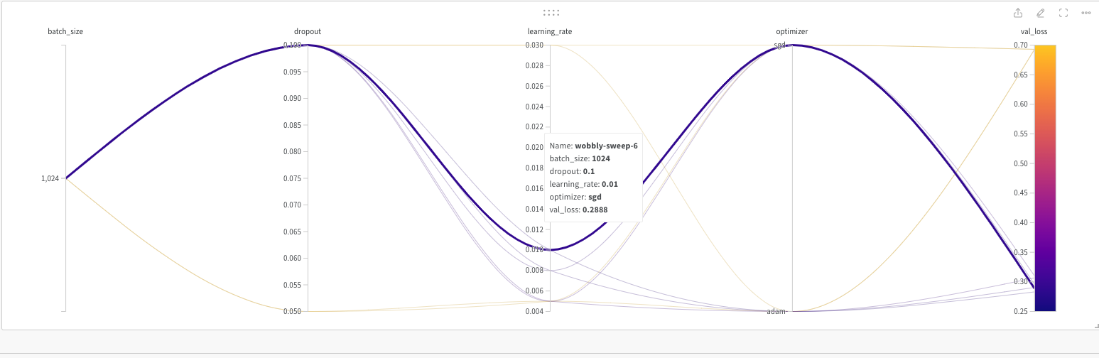
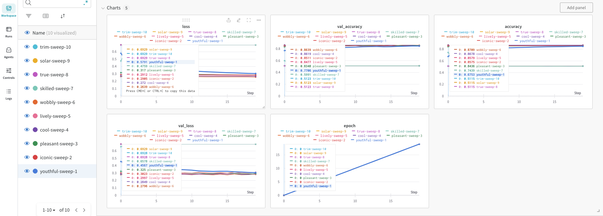
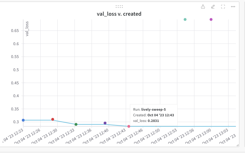
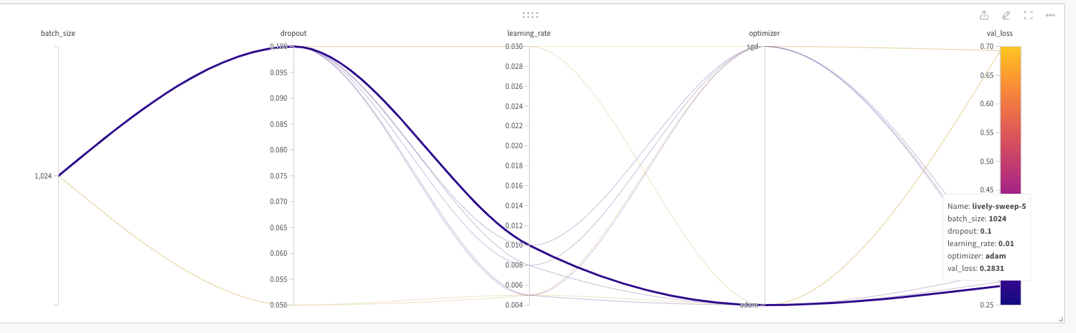
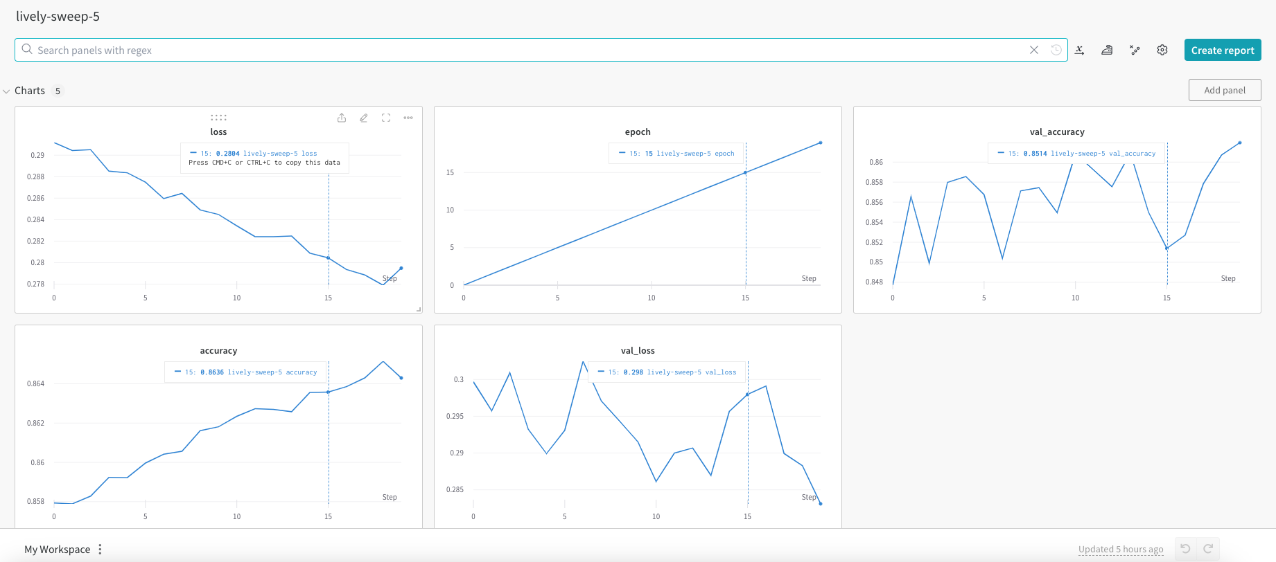
In the W & B site each of the runs or captured very nicely
The best model is ‘lively-sweep-5‘ with the lowest validation loss
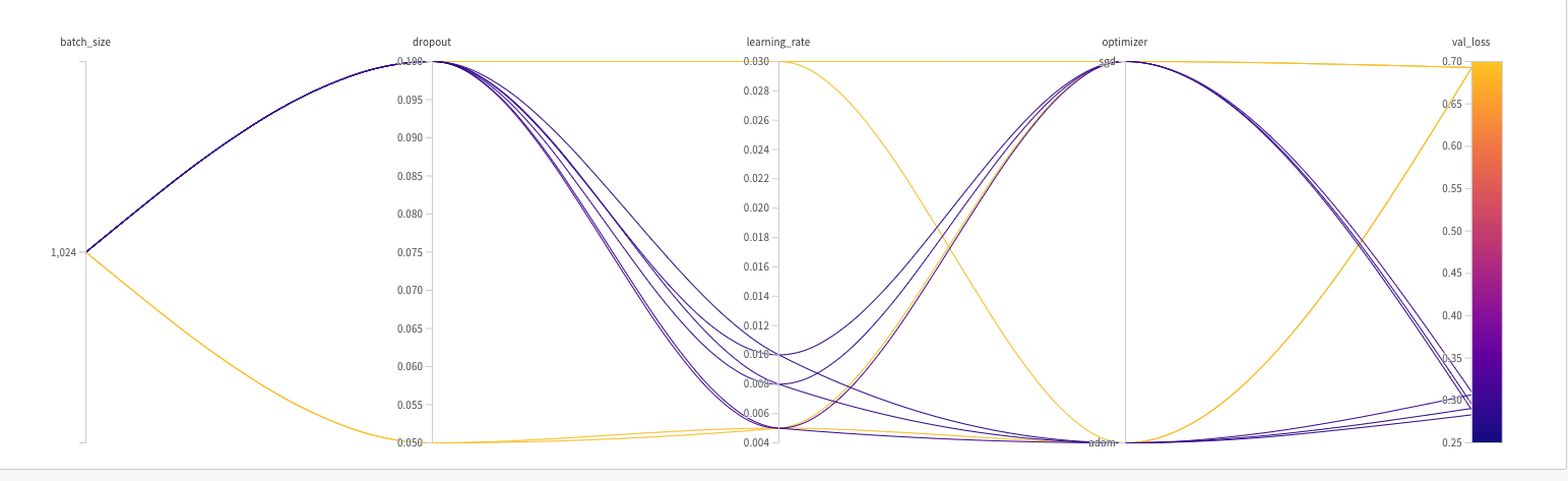
The picture below gives the validation loss for various combinations of the hyper-para meters
It is very easy to visually pick the best model with loss as shown below. It is lively-sweep-5. we can see the values of the hyper-parameters for this DL model
Details of optimal Deep Learning model
a. Run – lively-sweep-5
b. optimizer – adam
c. learning_rate – 0.01
d. batch_size – 1024
e. dropout – 0.1
We can see the performance of this model individually by clicking lively-sweep-6 on the left panel
It was good fun to play around with the Weights and Biases in selecting an optimal model
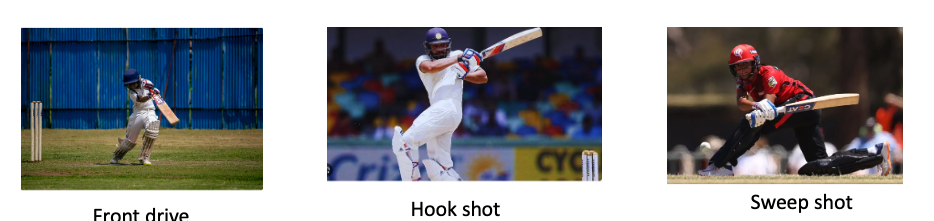
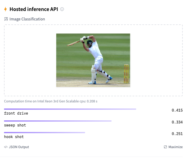
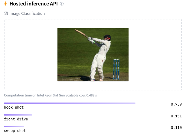
Image classification using Deep Learning has been around for almost a decade. In fact, this field with the use of Convolutional Neural Networks (CNN) is quite mature and the algorithms work very well in image classification, object detection, facial recognition and self-driving cars. In this post, I use AI image classification to identify cricketing shots. While the problem falls in a well known domain, the application of image classification in identifying cricketing shots is probably new. I have selected three cricketing shots, namely, the front drive, sweep shot, and the hook shot for this purpose. My purpose was to build a proof-of-concept and not a perfect product. I have kept the dataset deliberately small (for obvious reasons) of just about 14 samples for each cricketing shot, and for a total of about 41 total samples for both training and test data. Anyway, I get a reasonable performance from the AI model.
Included below are some examples of the data set
This post is based on this or on Image classification from Hugging face. Interestingly, this, the model used here is based on Vision Transformers (ViT from Google Brain) and not on Convolutional Neural Networks as is usually done.
The steps are to fine-tune ViT Transformer with the ‘strokes’ dataset are
d) Create a dictionary that maps the label name to an integer and vice versa. Display the labels
labels = df1.features["label"].names
label2id, id2label = dict(), dict()
for i, label in enumerate(labels):
label2id[label] = str(i)
id2label[str(i)] = label
labels
['front drive', 'hook shot', 'sweep shot']
e) Load ViT image processor. To apply the correct transformations, ImageProcessor is initialised with a configuration that was saved along with the pretrained model
from transformers import AutoImageProcessor
checkpoint = "google/vit-base-patch16-224-in21k"
image_processor = AutoImageProcessor.from_pretrained(checkpoint)
f) Apply image transformations to the images to make the model more robust against overfitting
from torchvision.transforms import RandomResizedCrop, Compose, Normalize, ToTensor
normalize = Normalize(mean=image_processor.image_mean, std=image_processor.image_std)
size = (
image_processor.size["shortest_edge"]
if "shortest_edge" in image_processor.size
else (image_processor.size["height"], image_processor.size["width"])
)
_transforms = Compose([RandomResizedCrop(size), ToTensor(), normalize])
g) Create a preprocessing function to apply the transforms and return pixel_values of the image as the inputs to the model – :
def transforms(examples):
examples["pixel_values"] = [_transforms(img.convert("RGB")) for img in examples["image"]]
del examples["image"]
return examples
h) Apply the preprocessing function over the entire dataset, using Hugging Face Dataset’s ‘with_transform’ method
df1 = df1.with_transform(transforms)
from transformers import DefaultDataCollator
data_collator = DefaultDataCollator()
As I mentioned before, the model should be reasonably accurate but not perfect, since my training dataset is extremely small. This is just a prototype to show that shot identification in cricket with AI is in the realm of the possible.
Ever since I started to use ChatGPT, I have been fascinated by its capabilities. To a large extent, the abilities of Large Language Models (LLMs) is quite magical – the way it answers questions, the way it summarises passages, the way it creates poems et cetera. All the LLMs need is a large corpus of data from the internet, articles, wikis, blogs, and so on.
On delving a little deeper into Generative AI, LLMs I learnt that, this is based on the principle of being able to predict the most probable word in a given sequence. It made me wonder whether the world of ideas, language and communication are actually governed by probabilities. Does what we communicate fall within the purview of statistics?
As an aside, just by extending further if we visualise a world in which every human action to a situation is assigned an embedding vector, and if we feed the responses of all humans over time in different situations, to the equivalent of a Transformer of a Large Human Reaction Model (LHRM) ;-), we can envisage the model being capable of predicting the response of human in a given situation. In my opinion, the machine would be fairly right most of the occasions as it could select the most probable choice of action, much like ‘The Machine’ in Person of Interest. However, this does not mean that the machine (AI) is actually more intelligent than humans. All it means is that the choice of humans responses are a part of a finite subset possibilities and The Machine (AI) can compute the possibilities and associated probabilities much quicker than humans. Does it mean that the world is deterministic? Possibly.
In this post, I use the T5 transformer to summarise Indian philosophy. For this task, I have fine-tuned the T5 model with a curated dataset taken from random passages on Hindu philosophy available on the internet. For each passage, I had to and hand-create the corresponding summary. This was a fairly tedious and demanding task but an enlightening one. It was interesting to understand how our ancestors, the Rishis, understood reality, the physical world, senses, the mind, the intellect, consciousness (Atman) and universal consciousness (Brahman). (Incidentally I was only able to curate only about 130 rows of philosophical snippets and manually create the corresponding summaries. Probably this is a very small dataset for fine-tuning but I just wanted to see the performance of the T5 model in a new domain.)
In this post the T5 model is fine-tuned with the curated dataset and the rouge1 and rouge2 scores are used to evaluate the model’s performance.
I have used the Hugging Face Hub for the transformer model, corresponding LLM functions and management of the dataset etc. The Hugging Face ecosystem is simply wow!!
 from huggingface_hub import notebook_login
notebook_login()

Login successful
c) Load the curated dataset on Hindu philosophy
from datasets import load_dataset
df1 = load_dataset("tvganesh/philosophy",split='train')
d) Load a T5 tokenizer to process text and summary
Prefix the input with a prompt so T5 knows this is a summarization task.
Use the keyword text_target argument when tokenizing labels.
Truncate sequences to be no longer than the maximum length set by the max_length parameter. The max_length of the text kept at 220 words and the max_length of the summary is kept at 50 words.
The ‘map’ function of the Huggingface dataset can be used to apply the pre_process function across the entire data.
DataCollatorForSeq2Seq can be used to dynamically pad the sentences to the longest length in a batch during collation, instead of padding the whole dataset to the maximum length.
from transformers import DataCollatorForSeq2Seq
data_collator = DataCollatorForSeq2Seq(tokenizer=tokenizer, model=checkpoint)
e) Evaluate performance of Model
The rouge1,rouge2 metric can be used to evaluate the performance of the model
import evaluate
rouge = evaluate.load("rouge")
f)Create a function compute_metrics that passes your predictions and labels to ‘compute’ to calculate the ROUGE metric:
import numpy as np

def compute_metrics(eval_pred):
    # evaluate predictions and labels
    predictions, labels = eval_pred
    decoded_preds = tokenizer.batch_decode(predictions, skip_special_tokens=True)
    labels = np.where(labels != -100, labels, tokenizer.pad_token_id)
    decoded_labels = tokenizer.batch_decode(labels, skip_special_tokens=True)
     # compute rouge score between the labels and predictions
    result = rouge.compute(predictions=decoded_preds, references=decoded_labels, use_stemmer=True)

    prediction_lens = [np.count_nonzero(pred != tokenizer.pad_token_id) for pred in predictions]
    result["gen_len"] = np.mean(prediction_lens)

    return {k: round(v, 4) for k, v in result.items()}
g) Split the data into training(80%) and test(20%) data set
from transformers import AutoModelForSeq2SeqLM, Seq2SeqTrainingArguments, Seq2SeqTrainer
model = AutoModelForSeq2SeqLM.from_pretrained(checkpoint)
i)
Set training hyperparameters in Seq2SeqTrainingArguments. The Adam optimization, with learning rate, beta1 & beta2 are used
Pass the training arguments to Seq2SeqTrainer along with the model, dataset, tokenizer, data collator, and compute_metrics function.
Call train() to finetune your model.
training_args = Seq2SeqTrainingArguments(
    output_dir="philosophy_model",
    evaluation_strategy="epoch",
    learning_rate= 5.6e-03,
    adam_beta1=0.9,
    adam_beta2=0.99,
    adam_epsilon=1e-06,
    per_device_train_batch_size=8,
    per_device_eval_batch_size=8,
    weight_decay=0.01,
    save_total_limit=3,
    num_train_epochs=20,
    predict_with_generate=True,
    fp16=True,
    push_to_hub=True,
)

trainer = Seq2SeqTrainer(
    model=model,
    args=training_args,
    train_dataset=train_dataset,
    eval_dataset=test_dataset,
    tokenizer=tokenizer,
    data_collator=data_collator,
    compute_metrics=compute_metrics,
)

trainer.train()

Epoch	Training Loss	Validation Loss	Rouge1	Rouge2	Rougel	Rougelsum	Gen Len
1	No log	2.246223	0.363200	0.146200	0.311400	0.312600	18.333300
2	No log	1.461140	0.459000	0.303900	0.417800	0.417800	18.566700
3	No log	0.832312	0.546500	0.425900	0.524700	0.520800	17.133300
4	No log	0.472341	0.616100	0.517600	0.601000	0.600400	18.366700
5	No log	0.312106	0.681200	0.607800	0.674700	0.671400	18.233300
6	No log	0.154585	0.741800	0.702300	0.733800	0.731300	18.066700
7	No log	0.112100	0.783200	0.763000	0.780200	0.778900	18.500000
8	No log	0.069882	0.801400	0.788200	0.802700	0.800900	18.533300
9	No log	0.045941	0.795800	0.780500	0.794600	0.791700	18.500000
10	No log	0.051655	0.809100	0.795800	0.810500	0.809000	18.466700
11	No log	0.035792	0.799400	0.785200	0.797300	0.794600	18.500000
12	No log	0.041766	0.779900	0.754800	0.774700	0.773200	18.266700
13	No log	0.010703	0.810000	0.800400	0.810700	0.809000	18.500000
14	No log	0.006519	0.807700	0.797100	0.809400	0.807500	18.500000
15	No log	0.017779	0.808000	0.796000	0.809400	0.807500	18.366700
16	No log	0.001681	0.810000	0.800400	0.810700	0.809000	18.500000
17	No log	0.005469	0.810000	0.800400	0.810700	0.809000	18.500000
18	No log	0.002003	0.810000	0.800400	0.810700	0.809000	18.500000
19	No log	0.000638	0.810000	0.800400	0.810700	0.809000	18.500000
20	No log	0.000498	0.810000	0.800400	0.810700	0.809000	18.500000
TrainOutput(global_step=260, training_loss=0.6491916949932391, metrics={'train_runtime': 57.99, 'train_samples_per_second': 34.489, 'train_steps_per_second': 4.484, 'total_flos': 101132046434304.0, 'train_loss': 0.6491916949932391, 'epoch': 20.0})
As we can see the rouge1 to rouge2 scores are fairly good. Anything above 0.5 is considered good. Maybe this is because the T5 model has already been pre-trained on a fairly large philosophical dataset
j) Push to hub
trainer.push_to_hub()
k) Summarise using pipeline
text = "summarize: A seeker who has the necessary qualifications, in order that he may be redeemed from his inner weaknesses, attachments, animalisms and false values is advised to serve with devotion a Teacher who is well- established in the experience of the Self."

from transformers import pipeline

summarizer = pipeline("summarization", model="tvganesh/philosophy_model")
summarizer(text)

[{'summary_text': 'A seeker who has the necessary qualifications will be able to free oneself of sense objects, and one cannot expect this to happen without any mental tossing'}]
l) Summarise using model generate
from transformers import AutoTokenizer

tokenizer = AutoTokenizer.from_pretrained("tvganesh/philosophy_model")
inputs = tokenizer(text, return_tensors="pt").input_ids

from transformers import AutoModelForSeq2SeqLM

model = AutoModelForSeq2SeqLM.from_pretrained("tvganesh/philosophy_model")
outputs = model.generate(inputs, max_new_tokens=70, do_sample=False)

tokenizer.decode(outputs[0], skip_special_tokens=True)

'A seeker who has the necessary qualifications will help in his journey to redeem himself'
l) Number of beams
summary_ids = model.generate(inputs,
                                    num_beams=10,
                                    no_repeat_ngram_size=3,
                                    min_length=20,
                                    max_length=70,
                                    early_stopping=True)
output = tokenizer.decode(summary_ids[0], skip_special_tokens=True)
output

'A seeker who has the necessary qualifications will be able to free himself of sense objects and false values'
I also tried Facebook’s BART Large model but the performance was not good at all.
You can try out the model at the following link philosophy_model
In this post, I revisit the visualisation of IPL batsman and bowler similarities using Google’s Embedding Projector. I had previously done this using multivariate regression in my earlier post ‘Using embeddings, collaborative filtering with Deep Learning to analyse T20 players.’ However, I was not too satisfied with the result since I was not getting the required accuracy.
This post uses the win-loss status of IPL matches from 2014 onwards upto 2023 in Logistic Regression with Deep Learning. A 16-dimensional embedding layer is added for the batsman and the bowler for ball-by-ball data. Since I have used a reduced size data set (from 2014) I get a slightly reduced accuracy, but still I think this is a well-formulated problem.
A Deep Learning network performs gradient descent based using Adam optimisation to arrive at an accuracy of 0.8047. The weights of the learnt Deep Learning network in ‘layer 0’ is used for displaying the batsman and bowler similarities.
Similarity measures –Cosine similarity
A cosine similarity is a value that is bound by a constrained range of 0 and 1. The closer the value is to 0 means that the two vectors are orthogonal or perpendicular to each other. When the value is closer to one, it means the angle is smaller and the batsman and bowler are similar.
a) Data set
For the data set only IPL T20 matches from Jan 2014 upto the present (May 2023) was taken. A Deep Learning model using Logistic Regression with batsman and bowler embedding is used to minimise the error. An accuracy of 0.8047 is obtained. In my earlier post ‘GooglyPlusPlus: Win Probability using Deep Learning and player embeddings‘ I had used data from all T20 leagues (~1.2 million rows) and got an accuracy of 0.8647
b) Import the data
import pandas as pd
import numpy as np
from zipfile import ZipFile
import tensorflow as tf
from tensorflow import keras
from tensorflow.keras import layers
from tensorflow.keras import regularizers
from pathlib import Path
import matplotlib.pyplot as plt

import pandas as pd
import numpy as np
from zipfile import ZipFile
import tensorflow as tf
from tensorflow import keras
from tensorflow.keras import layers
from tensorflow.keras import regularizers

df1=pd.read_csv('ipl2014_23.csv')
print("Shape of dataframe=",df1.shape)

train_dataset = df1.sample(frac=0.8,random_state=0)
test_dataset = df1.drop(train_dataset.index)
train_dataset1 = train_dataset[['batsmanIdx','bowlerIdx','ballNum','ballsRemaining','runs','runRate','numWickets','runsMomentum','perfIndex']]
test_dataset1 = test_dataset[['batsmanIdx','bowlerIdx','ballNum','ballsRemaining','runs','runRate','numWickets','runsMomentum','perfIndex']]
train_dataset1
train_labels = train_dataset.pop('isWinner')
test_labels = test_dataset.pop('isWinner')
train_dataset1

a=train_dataset1.describe()
stats=a.transpose

Shape of dataframe= (138896, 10)
batsmanIdx	bowlerIdx	ballNum	ballsRemaining	runs	runRate	numWickets	runsMomentum	perfIndex
count	111117.000000	111117.000000	111117.000000	111117.000000	111117.000000	111117.000000	111117.000000	111117.000000	111117.000000
mean	218.672939	169.204145	120.372067	60.749822	86.881701	1.636353	2.423167	0.296061	10.578927
std	118.405729	96.934754	69.991408	35.298794	51.643164	2.672564	2.085956	0.620872	4.436981
min	1.000000	1.000000	1.000000	1.000000	-5.000000	-5.000000	0.000000	0.057143	0.000000
25%	111.000000	89.000000	60.000000	30.000000	45.000000	1.160000	1.000000	0.106383	7.733333
50%	220.000000	170.000000	119.000000	60.000000	85.000000	1.375000	2.000000	0.142857	10.329545
75%	325.000000	249.000000	180.000000	91.000000	126.000000	1.640000	4.000000	0.240000	13.108696
max	411.000000	332.000000	262.000000	135.000000	258.000000	251.000000	10.000000	11.000000	66.000000
c) Create a Deep Learning ML model using batsman & bowler embeddings
import pandas as pd
import numpy as np
from keras.layers import Input, Embedding, Flatten, Dense
from keras.models import Model
from keras.layers import Input, Embedding, Flatten, Dense, Reshape, Concatenate, Dropout
from keras.models import Model

tf.random.set_seed(432)
# create input layers for each of the predictors
batsmanIdx_input = Input(shape=(1,), name='batsmanIdx')
bowlerIdx_input = Input(shape=(1,), name='bowlerIdx')
ballNum_input = Input(shape=(1,), name='ballNum')
ballsRemaining_input = Input(shape=(1,), name='ballsRemaining')
runs_input = Input(shape=(1,), name='runs')
runRate_input = Input(shape=(1,), name='runRate')
numWickets_input = Input(shape=(1,), name='numWickets')
runsMomentum_input = Input(shape=(1,), name='runsMomentum')
perfIndex_input = Input(shape=(1,), name='perfIndex')

# Set the embedding size
no_of_unique_batman=len(df1["batsmanIdx"].unique())
print(no_of_unique_batman)
no_of_unique_bowler=len(df1["bowlerIdx"].unique())
print(no_of_unique_bowler)
embedding_size_bat = no_of_unique_batman ** (1/4)
embedding_size_bwl = no_of_unique_bowler ** (1/4)


# create embedding layer for the categorical predictor
batsmanIdx_embedding = Embedding(input_dim=no_of_unique_batman+1, output_dim=16,input_length=1)(batsmanIdx_input)
batsmanIdx_flatten = Flatten()(batsmanIdx_embedding)
bowlerIdx_embedding = Embedding(input_dim=no_of_unique_bowler+1, output_dim=16,input_length=1)(bowlerIdx_input)
bowlerIdx_flatten = Flatten()(bowlerIdx_embedding)

# concatenate all the predictors
x = keras.layers.concatenate([batsmanIdx_flatten,bowlerIdx_flatten, ballNum_input, ballsRemaining_input, runs_input, runRate_input, numWickets_input, runsMomentum_input, perfIndex_input])

# add hidden layers
#x = Dense(64, activation='relu')(x)
#x = Dropout(0.1)(x)
x = Dense(32, activation='relu')(x)
x = Dropout(0.1)(x)
x = Dense(16, activation='relu')(x)
x = Dropout(0.1)(x)
x = Dense(8, activation='relu')(x)
x = Dropout(0.1)(x)
# add output layer
output = Dense(1, activation='sigmoid', name='output')(x)
print(output.shape)
# create model
model = Model(inputs=[batsmanIdx_input,bowlerIdx_input, ballNum_input, ballsRemaining_input, runs_input, runRate_input, numWickets_input, runsMomentum_input, perfIndex_input], outputs=output)
model.summary()

# compile model
optimizer=keras.optimizers.Adam(learning_rate=.01, beta_1=0.9, beta_2=0.999, epsilon=1e-07, amsgrad=True)

model.compile(optimizer=optimizer, loss='binary_crossentropy', metrics=['accuracy'])

# train the model
history=model.fit([train_dataset1['batsmanIdx'],train_dataset1['bowlerIdx'],train_dataset1['ballNum'],train_dataset1['ballsRemaining'],train_dataset1['runs'],
           train_dataset1['runRate'],train_dataset1['numWickets'],train_dataset1['runsMomentum'],train_dataset1['perfIndex']], train_labels, epochs=40, batch_size=1024,
          validation_data = ([test_dataset1['batsmanIdx'],test_dataset1['bowlerIdx'],test_dataset1['ballNum'],test_dataset1['ballsRemaining'],test_dataset1['runs'],
           test_dataset1['runRate'],test_dataset1['numWickets'],test_dataset1['runsMomentum'],test_dataset1['perfIndex']],test_labels), verbose=1)

plt.plot(history.history["loss"])
plt.plot(history.history["val_loss"])
plt.title("model loss")
plt.ylabel("loss")
plt.xlabel("epoch")
plt.legend(["train", "test"], loc="upper left")
plt.show()
d) Project embeddings with Google’s Embedding projector
try:
  # %tensorflow_version only exists in Colab.
  %tensorflow_version 2.x
except Exception:
  pass

%load_ext tensorboard
import os
import tensorflow as tf
import tensorflow_datasets as tfds
from tensorboard.plugins import projector

%pwd
# Set up a logs directory, so Tensorboard knows where to look for files.
log_dir='/logs/batsmen/'
if not os.path.exists(log_dir):
    os.makedirs(log_dir)

df3=pd.read_csv('batsmen.csv')
batsmen = df3["batsman"].unique().tolist()
batsmen
# Create dictionary of batsman to index
batsmen2index = {x: i for i, x in enumerate(batsmen)}
batsmen2index
# Create dictionary of index to batsman
index2batsmen = {i: x for i, x in enumerate(batsmen)}
index2batsmen


# Save Labels separately on a line-by-line manner.
with open(os.path.join(log_dir, 'metadata.tsv'), "w") as f:
  for batsmanIdx in range(1, 411):
       # Get the name of batsman associated at the current index
        batsman = index2batsmen.get([batsmanIdx][0])

        f.write("{}\n".format(batsman))

# Save the weights we want to analyze as a variable. Note that the first
# value represents any unknown word, which is not in the metadata, here
# we will remove this value.
weights = tf.Variable(model.get_weights()[0][1:])
print(weights)
print(type(weights))
print(len(model.get_weights()[0]))
# Create a checkpoint from embedding, the filename and key are the
# name of the tensor.
checkpoint = tf.train.Checkpoint(embedding=weights)
checkpoint.save(os.path.join(log_dir, "embedding.ckpt"))

# Set up config.
config = projector.ProjectorConfig()
embedding = config.embeddings.add()
# The name of the tensor will be suffixed by `/.ATTRIBUTES/VARIABLE_VALUE`.
embedding.tensor_name = "embedding/.ATTRIBUTES/VARIABLE_VALUE"
embedding.metadata_path = 'metadata.tsv'
projector.visualize_embeddings(log_dir, config)
# Now run tensorboard against on log data we just saved.

%reload_ext tensorboard
%tensorboard --logdir /logs/batsmen/
e) Here are similarity measures for some batsmen
I) Principal Component Analysis (PCA) : In the charts and video animation below, the 16-dimensional embedding vector of batsmen and bowler is reduced to 3 principal components in a lower dimension for visualisation and analysis as shown below
a) Yashasvi Jaiswal (similar players
i) PCA – Chart
Yashasvi Jaiswal style of attack is similar to Faf Du Plessis, Quentim De Kock, Bravo etc. In the below chart the ange between Jaiswal and SP Narine is 0.109, and Faf du Plessis is 0.253. These represent the angle in radians. The smaller the angle the more similar the performance style of the players and cos 0=1 or the players are similar.
ii) PCA animation video for Yashasvi Jaiswal
b) Suryakumar Yadav (SKY)
i) PCA -Chart
The closest neighbours for SKY is RV Uthappa, Rahul Tripathi, Q de Kock, Samson, Rashid Khan
ii) PCA – Animation video for Suryakumar Yadav
c) M S Dhoni
i) PCA – Chart
Dhoni rubs shoulders with Bravo, AB De Villiers, Shane Watson, Chris Gayle, Rayadu, Gautam Gambhir
ii) PCA – Animation video for M S Dhoni
f) PCA Analysis for bowlers
a) Jasprit Bumrah
i) PCA – Chart
Bumrah bowling performance is similar to Josh Hazzlewood, Chameera, Kuldeep Yadav, Nortje, Adam Zampa etc.
ii) PCA Animation video for Jasprit Bumrah
b) Yuzhvendra Chahal
i) PCA – Chart
Chahal’s performance has a strong similarity to Malinga, Zaheer Khan, Imran Tahir, R Sheperd, Adil Rashid
ii) PCA Animation video for YS Chahal
f) Other similarity measures ( t-SNE & UMAP)
There are 2 other similarity visualisations in Google’s Embedding Projector namely
i) t-SNE (t-distributed Stochastic Neighbor Embedding) – t-SNE tries to find a faithful representation of the data distribution in higher dimensional space to a lower dimensional space. t-SNE differs from PCA by preserving only or local similarities whereas PCA is maintains preserving large pairwise distances.
a) t-SNE Animationvideo
ii) UMAP – Uniform Manifold Approximation and Projection
UMAP learns the manifold structure of the high dimensional data and finds a low dimensional embedding that preserves the essential topological structure of that manifold.
ii) UMAP – Animationvideo
The Embedding projector thus helps in identifying players based on how they perform against bowlers, and probably picks up a lot of features like strike rate and performance in different stages of the game.
“The unexamined life is not worth living.” – Socrates
“There is no easy way from the earth to the stars.” – Seneca
“If you want to go fast, go alone. If you want to go far, go together.” – African Proverb
1. Introduction
In this post, I put my R package cricketr to analyze the Indian and Australia World Test Championship (WTC) final squad ahead of the World Test Championship 2023.My R package cricketr had its birth on Jul 4, 2015. Cricketr uses data from Cricinfo.
According to me, Ishan Kishan has more experience than KS Bharat, though Rishabh Pant would have been the ideal wicket keeper/left-handed batsman. I think Shardul Thakur would be handful in the English conditions. For a spinner it either Ashwin or Jadeja. Maybe the balance shifts in favor of Jadeja
Australian squad
Pat Cummins (capt), Alex Carey (wk), Cameron Green, Josh Hazlewood, Usman Khawaja, Marnus Labuschagne, Nathan Lyon, Todd Murphy, Steven Smith (vice-capt), Mitchell Starc, David Warner.
Not sure if Scott Boland would fill in, instead of Todd Murphy 1
Let me give you a lay-of-the-land (post) below
The post below is organized into the following parts
Analysis of Indian WTC batsmen from Jan 2016 – May 2023
Analysis of Indian WTC batsmen against Australia from Jan 2016 -May 2023
Analysis of Australian WTC batsmen from Jan 2016 – May 2023
Analysis of Australian WTC batsmen against India from Jan 2016 -May 2023
Analysis of Indian WTC bowlers from Jan 2016 – May 2023
Analysis of Indian WTC bowlers against Australia from Jan 2016 -May 2023
Analysis of Australian WTC bowlers from Jan 2016 – May 2023
Analysis of Australian WTC bowlers gainst India from Jan 2016 -May 2023
Team analysis of India and Australia
All the above analysis use data from ESPN Statsguru and use my R pakage cricketr
The data for the different players have been obtained using calls such as the ones below.
# Get Shubman Gill's batting data
#shubman <-getPlayerData(1070173,dir=".",file="shubman.csv",type="batting",homeOrAway=c(1,2), result=c(1,2,4))
#shubmansp <- getPlayerDataSp(1070173,tdir=".",tfile="shubmansp.csv",ttype="batting")

#Get Shubman Gill's data from Jan 2016 - May 2023
#df <-getPlayerDataHA(1070173,tfile="shubman1.csv",type="batting", matchType="Test")
#df1=getPlayerDataOppnHA(infile="shubman1.csv",outfile="shubmanTestAus.csv",startDate="2016-01-01",endDate="2023-05-01")

#Get Shubman Gills data from Jan 2016 - May 2023, against Australia
#df <-getPlayerDataHA(1070173,tfile="shubman1.csv",type="batting", matchType="Test")
#df1=getPlayerDataOppnHA(infile="shubman1.csv",outfile="shubmanTestAus.csv",opposition="Australia",startDate="2016-01-01",endDate="2023-05-01")
Note: To get data for bowlers we need to use the corresponding profile no and use type =‘bowling’. Details in my posts below
To do similar analysis please go through the following posts
Note 1: I will not be analysing each and every chart as the charts are quite self-explanatory
Note 2: I have had to tile charts together otherwise this will become a very, very long post. You are free to use my R package cricketr and check out for yourself ##3. Analysis of India WTC batsmen from Jan 2016 – May 2023
Findings
Kohli has the best average of 48+. India has won when Rohit and Rahane played well
Kohli’s tops the list in cumulative average runs, followed by Pujara and Rohit is 3rd. Gill is on the upswing.
Against Australia Pujara has the best cumulative average runs record followed by Rahane, with Gill in hot pursuit. In the strike rate department Gill tops followed by Rohit and Rahane
Since 2016 Smith, Labuschagne has an average of 53+ since 2016!! Warner & Khwaja are at ~46
Australia has won matches when Smith, Warner and Khwaja have played well.
Labuschagne, Smith and C Green have good records against India. Indian bowlers will need to contain them
Ashwin has the highest wickets followed by Jadeja against all teams. Ashwin’s performance has dropped over the years, while Siraj has been becoming better
Jadeja has the best economy rate followed by Ashwin
Against Australia specifically Jadeja has the best record followed by Ashwin. Jadeja has the best economy against Australia, followed by Siraj, then Ashwin
Cummins, Starc and Lyons are the best performers for Australia. Hazzlewood, Cummins have the best economy against all opposition
Against India Lyon, Cummins and Hazzlewood have performed well
Hazzlewood, Lyon have a good economy rate against India
Against Australia India has won 17 times, lost 60 and drawn 22 in Australia. At home India won 42, tied 2, lost 28 and drawn 24
At the Oval where the World Test Championship is going to be held India has won 4, lost 10 and drawn 10.
Note 3: You can also read this post at Rpubs at ind-aus-WTC!! The formatting will be nicer!
Note 4: You can download this post as PDF to read at your leisure ind-aus-WTC.pdf
2. Install the cricketr package
if (!require("cricketr")){
    install.packages("cricketr",lib = "c:/test")
}
library(cricketr)
3a. Basic analysis
The analyses below include – Runs frequency plot – Mean strike rate – Run Ranges
Kohli’s strike rate increases with increasing runs, while Gill’s seems to drop. So it is with Pujara & Rahane
This plot shows a combined boxplot of the Runs ranges and a histog2ram of the Runs Frequency Kohli’s average is 48, while Rohit,Pujara is 40 with Rahane and Gill around 33.
batsmanPerfBoxHist("kohliTest.csv","Kohli")
batsmanPerfBoxHist("rohitTest.csv","Rohit")
batsmanPerfBoxHist("shubmanTest.csv","S Gill")
batsmanPerfBoxHist("rahaneTest.csv","Rahane")
batsmanPerfBoxHist("pujaraTest.csv","Pujara")
3d. Contribution to won and lost matches
For the functions below you will have to use the getPlayerDataSp() function. When Rohit Sharma and Pujara have played well India have tended to win more often
## Summary of  Kohli 's runs scoring likelihood
## **************************************************
##
## There is a 52.91 % likelihood that Kohli  will make  12 Runs in  26 balls over 35  Minutes
## There is a 30.81 % likelihood that Kohli  will make  52 Runs in  100 balls over  139  Minutes
## There is a 16.28 % likelihood that Kohli  will make  142 Runs in  237 balls over 335  Minutes
batsmanRunsLikelihood("rohit.csv","Rohit")
## Summary of  Rohit 's runs scoring likelihood
## **************************************************
##
## There is a 43.24 % likelihood that Rohit  will make  10 Runs in  21 balls over 32  Minutes
## There is a 45.95 % likelihood that Rohit  will make  46 Runs in  85 balls over  124  Minutes
## There is a 10.81 % likelihood that Rohit  will make  110 Runs in  199 balls over 282  Minutes
batsmanRunsLikelihood("rahane.csv","Rahane")
## Summary of  Rahane 's runs scoring likelihood
## **************************************************
##
## There is a 7.75 % likelihood that Rahane  will make  124 Runs in  224 balls over 318  Minutes
## There is a 62.02 % likelihood that Rahane  will make  12 Runs in  26 balls over  37  Minutes
## There is a 30.23 % likelihood that Rahane  will make  55 Runs in  113 balls over 162  Minutes
batsmanRunsLikelihood("pujara.csv","Pujara")
## Summary of  Pujara 's runs scoring likelihood
## **************************************************
##
## There is a 60.49 % likelihood that Pujara  will make  15 Runs in  38 balls over 55  Minutes
## There is a 31.48 % likelihood that Pujara  will make  62 Runs in  142 balls over  204  Minutes
## There is a 8.02 % likelihood that Pujara  will make  153 Runs in  319 balls over 445  Minutes
3h1. Moving average of batsman
Kohli’s moving average in tests seem to havw dropped after a peak in 2017, 2018. So it is with Rahane
Here are plots that forecast how the batsman will perform in future. In this case 90% of the career runs trend is uses as the training set. the remaining 10% is the test set.
A Holt-Winters forecating model is used to forecast future performance based on the 90% training set. The forecated runs trend is plotted. The test set is also plotted to see how close the forecast and the actual matches
Take a look at the runs forecasted for the batsman below.
The below computation uses Null Hypothesis testing and p-value to determine if the batsman is in-form or out-of-form. For this 90% of the career runs is chosen as the population and the mean computed. The last 10% is chosen to be the sample set and the sample Mean and the sample Standard Deviation are caculated.
The Null Hypothesis (H0) assumes that the batsman continues to stay in-form where the sample mean is within 95% confidence interval of population mean The Alternative (Ha) assumes that the batsman is out of form the sample mean is beyond the 95% confidence interval of the population mean.
A significance value of 0.05 is chosen and p-value us computed If p-value >= .05 – Batsman In-Form If p-value < 0.05 – Batsman Out-of-Form
Note Ideally the p-value should be done for a population that follows the Normal Distribution. But the runs population is usually left skewed. So some correction may be needed. I will revisit this later
This is done for the Top 4 batsman
checkBatsmanInForm("kohli.csv","Kohli")
## [1] "**************************** Form status of Kohli ****************************\n\n Population size: 154 Mean of population: 47.03 \n Sample size: 18 Mean of sample: 32.22 SD of sample: 42.45 \n\n Null hypothesis H0 : Kohli 's sample average is within 95% confidence interval of population average\n Alternative hypothesis Ha : Kohli 's sample average is below the 95% confidence interval of population average\n\n Kohli 's Form Status: In-Form because the p value: 0.078058 is greater than alpha= 0.05 \n *******************************************************************************************\n\n"
checkBatsmanInForm("rohit.csv","Rohit")
## [1] "**************************** Form status of Rohit ****************************\n\n Population size: 66 Mean of population: 37.03 \n Sample size: 8 Mean of sample: 37.88 SD of sample: 35.38 \n\n Null hypothesis H0 : Rohit 's sample average is within 95% confidence interval of population average\n Alternative hypothesis Ha : Rohit 's sample average is below the 95% confidence interval of population average\n\n Rohit 's Form Status: In-Form because the p value: 0.526254 is greater than alpha= 0.05 \n *******************************************************************************************\n\n"
checkBatsmanInForm("rahane.csv","Rahane")
## [1] "**************************** Form status of Rahane ****************************\n\n Population size: 116 Mean of population: 34.78 \n Sample size: 13 Mean of sample: 21.38 SD of sample: 21.96 \n\n Null hypothesis H0 : Rahane 's sample average is within 95% confidence interval of population average\n Alternative hypothesis Ha : Rahane 's sample average is below the 95% confidence interval of population average\n\n Rahane 's Form Status: Out-of-Form because the p value: 0.023244 is less than alpha= 0.05 \n *******************************************************************************************\n\n"
checkBatsmanInForm("pujara.csv","Pujara")
## [1] "**************************** Form status of Pujara ****************************\n\n Population size: 145 Mean of population: 41.93 \n Sample size: 17 Mean of sample: 33.24 SD of sample: 31.74 \n\n Null hypothesis H0 : Pujara 's sample average is within 95% confidence interval of population average\n Alternative hypothesis Ha : Pujara 's sample average is below the 95% confidence interval of population average\n\n Pujara 's Form Status: In-Form because the p value: 0.137319 is greater than alpha= 0.05 \n *******************************************************************************************\n\n"
checkBatsmanInForm("shubman.csv","S Gill")
## [1] "**************************** Form status of S Gill ****************************\n\n Population size: 23 Mean of population: 30.43 \n Sample size: 3 Mean of sample: 51.33 SD of sample: 66.88 \n\n Null hypothesis H0 : S Gill 's sample average is within 95% confidence interval of population average\n Alternative hypothesis Ha : S Gill 's sample average is below the 95% confidence interval of population average\n\n S Gill 's Form Status: In-Form because the p value: 0.687033 is greater than alpha= 0.05 \n *******************************************************************************************\n\n"
3q. Predicting Runs given Balls Faced and Minutes at Crease
A multi-variate regression plane is fitted between Runs and Balls faced +Minutes at crease.
4. Analysis of India WTC batsmen from Jan 2016 – May 2023 against Australia
4a. Relative cumulative average
Against Australia specifically between 2016 – 2023, Pujara has the best record followed by Rahane, with Gill in hot pursuit. Kohli and Rohit trail behind
For the 2 functions below you will have to use the getPlayerDataSp() function. Australia has won matches when Smith, Warner and Khwaja have played well.
## Summary of  S Smith 's runs scoring likelihood
## **************************************************
##
## There is a 58.76 % likelihood that S Smith  will make  21 Runs in  38 balls over 56  Minutes
## There is a 24.74 % likelihood that S Smith  will make  70 Runs in  148 balls over  210  Minutes
## There is a 16.49 % likelihood that S Smith  will make  148 Runs in  268 balls over 398  Minutes
batsmanRunsLikelihood("warnerTest.csv","Warner")
## Summary of  Warner 's runs scoring likelihood
## **************************************************
##
## There is a 7.22 % likelihood that Warner  will make  155 Runs in  253 balls over 372  Minutes
## There is a 62.89 % likelihood that Warner  will make  14 Runs in  21 balls over  32  Minutes
## There is a 29.9 % likelihood that Warner  will make  65 Runs in  94 balls over 135  Minutes
## Summary of  M Labuschagne 's runs scoring likelihood
## **************************************************
##
## There is a 32.76 % likelihood that M Labuschagne  will make  74 Runs in  144 balls over 206  Minutes
## There is a 55.17 % likelihood that M Labuschagne  will make  22 Runs in  37 balls over  54  Minutes
## There is a 12.07 % likelihood that M Labuschagne  will make  168 Runs in  297 balls over 420  Minutes
batsmanRunsLikelihood("khwajaTest.csv","Khwaja")
## Summary of  Khwaja 's runs scoring likelihood
## **************************************************
##
## There is a 64.94 % likelihood that Khwaja  will make  14 Runs in  29 balls over 42  Minutes
## There is a 27.27 % likelihood that Khwaja  will make  79 Runs in  148 balls over  210  Minutes
## There is a 7.79 % likelihood that Khwaja  will make  165 Runs in  351 balls over 515  Minutes
5i. Moving average of batsman
Smith and Warner’s moving average has been on a downward trend lately. Khwaja is playing well
Here are plots that forecast how the batsman will perform in future. In this case 90% of the career runs trend is uses as the training set. the remaining 10% is the test set.
A Holt-Winters forecating model is used to forecast future performance based on the 90% training set. The forecated runs trend is plotted. The test set is also plotted to see how close the forecast and the actual matches
Take a look at the runs forecasted for the batsman below.
The below computation uses Null Hypothesis testing and p-value to determine if the batsman is in-form or out-of-form. For this 90% of the career runs is chosen as the population and the mean computed. The last 10% is chosen to be the sample set and the sample Mean and the sample Standard Deviation are caculated.
The Null Hypothesis (H0) assumes that the batsman continues to stay in-form where the sample mean is within 95% confidence interval of population mean The Alternative (Ha) assumes that the batsman is out of form the sample mean is beyond the 95% confidence interval of the population mean.
A significance value of 0.05 is chosen and p-value us computed If p-value >= .05 – Batsman In-Form If p-value < 0.05 – Batsman Out-of-Form
Note Ideally the p-value should be done for a population that follows the Normal Distribution. But the runs population is usually left skewed. So some correction may be needed. I will revisit this later
This is done for the Top 4 batsman
checkBatsmanInForm("stevesmith.csv","S Smith")
## [1] "**************************** Form status of S Smith ****************************\n\n Population size: 144 Mean of population: 53.76 \n Sample size: 17 Mean of sample: 45.65 SD of sample: 56.4 \n\n Null hypothesis H0 : S Smith 's sample average is within 95% confidence interval of population average\n Alternative hypothesis Ha : S Smith 's sample average is below the 95% confidence interval of population average\n\n S Smith 's Form Status: In-Form because the p value: 0.280533 is greater than alpha= 0.05 \n *******************************************************************************************\n\n"
checkBatsmanInForm("warner.csv","Warner")
## [1] "**************************** Form status of Warner ****************************\n\n Population size: 164 Mean of population: 45.2 \n Sample size: 19 Mean of sample: 26.63 SD of sample: 44.62 \n\n Null hypothesis H0 : Warner 's sample average is within 95% confidence interval of population average\n Alternative hypothesis Ha : Warner 's sample average is below the 95% confidence interval of population average\n\n Warner 's Form Status: Out-of-Form because the p value: 0.042744 is less than alpha= 0.05 \n *******************************************************************************************\n\n"
## [1] "**************************** Form status of M Labuschagne ****************************\n\n Population size: 52 Mean of population: 59.56 \n Sample size: 6 Mean of sample: 29.67 SD of sample: 19.96 \n\n Null hypothesis H0 : M Labuschagne 's sample average is within 95% confidence interval of population average\n Alternative hypothesis Ha : M Labuschagne 's sample average is below the 95% confidence interval of population average\n\n M Labuschagne 's Form Status: Out-of-Form because the p value: 0.005239 is less than alpha= 0.05 \n *******************************************************************************************\n\n"
checkBatsmanInForm("khwaja.csv","Khwaja")
## [1] "**************************** Form status of Khwaja ****************************\n\n Population size: 89 Mean of population: 41.62 \n Sample size: 10 Mean of sample: 53.1 SD of sample: 76.34 \n\n Null hypothesis H0 : Khwaja 's sample average is within 95% confidence interval of population average\n Alternative hypothesis Ha : Khwaja 's sample average is below the 95% confidence interval of population average\n\n Khwaja 's Form Status: In-Form because the p value: 0.677691 is greater than alpha= 0.05 \n *******************************************************************************************\n\n"
5r. Predicting Runs given Balls Faced and Minutes at Crease
A multi-variate regression plane is fitted between Runs and Balls faced +Minutes at crease.
Here are plots that forecast how the bowler will perform in future. In this case 90% of the career wickets trend is used as the training set. the remaining 10% is the test set.
A Holt-Winters forecasting model is used to forecast future performance based on the 90% training set. The forecasted wickets trend is plotted. The test set is also plotted to see how close the forecast and the actual matches
The below computation uses Null Hypothesis testing and p-value to determine if the bowler is in-form or out-of-form. For this 90% of the career wickets is chosen as the population and the mean computed. The last 10% is chosen to be the sample set and the sample Mean and the sample Standard Deviation are caculated.
The Null Hypothesis (H0) assumes that the bowler continues to stay in-form where the sample mean is within 95% confidence interval of population mean The Alternative (Ha) assumes that the bowler is out of form the sample mean is beyond the 95% confidence interval of the population mean.
A significance value of 0.05 is chosen and p-value us computed If p-value >= .05 – Batsman In-Form If p-value < 0.05 – Batsman Out-of-Form
Note Ideally the p-value should be done for a population that follows the Normal Distribution. But the runs population is usually left skewed. So some correction may be needed. I will revisit this later
Note: The check for the form status of the bowlers indicate
checkBowlerInForm("shami.csv","Shami")
## [1] "**************************** Form status of Shami ****************************\n\n Population size: 106 Mean of population: 1.93 \n Sample size: 12 Mean of sample: 1.33 SD of sample: 1.23 \n\n Null hypothesis H0 : Shami 's sample average is within 95% confidence interval \n of population average\n Alternative hypothesis Ha : Shami 's sample average is below the 95% confidence\n interval of population average\n\n Shami 's Form Status: In-Form because the p value: 0.058427 is greater than alpha= 0.05 \n *******************************************************************************************\n\n"
checkBowlerInForm("siraj.csv","Siraj")
## [1] "**************************** Form status of Siraj ****************************\n\n Population size: 29 Mean of population: 1.59 \n Sample size: 4 Mean of sample: 0.25 SD of sample: 0.5 \n\n Null hypothesis H0 : Siraj 's sample average is within 95% confidence interval \n of population average\n Alternative hypothesis Ha : Siraj 's sample average is below the 95% confidence\n interval of population average\n\n Siraj 's Form Status: Out-of-Form because the p value: 0.002923 is less than alpha= 0.05 \n *******************************************************************************************\n\n"
checkBowlerInForm("ashwin.csv","Ashwin")
## [1] "**************************** Form status of Ashwin ****************************\n\n Population size: 154 Mean of population: 2.77 \n Sample size: 18 Mean of sample: 2.44 SD of sample: 1.76 \n\n Null hypothesis H0 : Ashwin 's sample average is within 95% confidence interval \n of population average\n Alternative hypothesis Ha : Ashwin 's sample average is below the 95% confidence\n interval of population average\n\n Ashwin 's Form Status: In-Form because the p value: 0.218345 is greater than alpha= 0.05 \n *******************************************************************************************\n\n"
checkBowlerInForm("jadeja.csv","Jadeja")
## [1] "**************************** Form status of Jadeja ****************************\n\n Population size: 108 Mean of population: 2.22 \n Sample size: 12 Mean of sample: 1.92 SD of sample: 2.35 \n\n Null hypothesis H0 : Jadeja 's sample average is within 95% confidence interval \n of population average\n Alternative hypothesis Ha : Jadeja 's sample average is below the 95% confidence\n interval of population average\n\n Jadeja 's Form Status: In-Form because the p value: 0.333095 is greater than alpha= 0.05 \n *******************************************************************************************\n\n"
checkBowlerInForm("shardul.csv","Shardul")
## [1] "**************************** Form status of Shardul ****************************\n\n Population size: 13 Mean of population: 2 \n Sample size: 2 Mean of sample: 0.5 SD of sample: 0.71 \n\n Null hypothesis H0 : Shardul 's sample average is within 95% confidence interval \n of population average\n Alternative hypothesis Ha : Shardul 's sample average is below the 95% confidence\n interval of population average\n\n Shardul 's Form Status: Out-of-Form because the p value: 0.04807 is less than alpha= 0.05 \n *******************************************************************************************\n\n"
8. Analysis of India WTC bowlers from Jan 2016 – May 2023 against Australia
8a Relative cumulative average wickets of bowlers in career
Against Australia specifically Jadeja has the best record followed by Ashwin
Here are plots that forecast how the bowler will perform in future. In this case 90% of the career wickets trend is used as the training set. the remaining 10% is the test set.
A Holt-Winters forecasting model is used to forecast future performance based on the 90% training set. The forecated wickets trend is plotted. The test set is also plotted to see how close the forecast and the actual matches
The below computation uses Null Hypothesis testing and p-value to determine if the bowler is in-form or out-of-form. For this 90% of the career wickets is chosen as the population and the mean computed. The last 10% is chosen to be the sample set and the sample Mean and the sample Standard Deviation are calculated.
The Null Hypothesis (H0) assumes that the bowler continues to stay in-form where the sample mean is within 95% confidence interval of population mean The Alternative (Ha) assumes that the bowler is out of form the sample mean is beyond the 95% confidence interval of the population mean.
A significance value of 0.05 is chosen and p-value us computed If p-value >= .05 – Batsman In-Form If p-value < 0.05 – Batsman Out-of-Form
Note Ideally the p-value should be done for a population that follows the Normal Distribution. But the runs population is usually left skewed. So some correction may be needed. I will revisit this later
Note: The check for the form status of the bowlers indicate
checkBowlerInForm("cummins.csv","Cummins")
## [1] "**************************** Form status of Cummins ****************************\n\n Population size: 81 Mean of population: 2.46 \n Sample size: 9 Mean of sample: 2 SD of sample: 1.5 \n\n Null hypothesis H0 : Cummins 's sample average is within 95% confidence interval \n of population average\n Alternative hypothesis Ha : Cummins 's sample average is below the 95% confidence\n interval of population average\n\n Cummins 's Form Status: In-Form because the p value: 0.190785 is greater than alpha= 0.05 \n *******************************************************************************************\n\n"
checkBowlerInForm("starc.csv","Starc")
## [1] "**************************** Form status of Starc ****************************\n\n Population size: 126 Mean of population: 2.18 \n Sample size: 15 Mean of sample: 1.67 SD of sample: 1.18 \n\n Null hypothesis H0 : Starc 's sample average is within 95% confidence interval \n of population average\n Alternative hypothesis Ha : Starc 's sample average is below the 95% confidence\n interval of population average\n\n Starc 's Form Status: In-Form because the p value: 0.057433 is greater than alpha= 0.05 \n *******************************************************************************************\n\n"
checkBowlerInForm("hazzlewood.csv","Hazzlewood")
## [1] "**************************** Form status of Hazzlewood ****************************\n\n Population size: 99 Mean of population: 2.04 \n Sample size: 12 Mean of sample: 1.67 SD of sample: 1.5 \n\n Null hypothesis H0 : Hazzlewood 's sample average is within 95% confidence interval \n of population average\n Alternative hypothesis Ha : Hazzlewood 's sample average is below the 95% confidence\n interval of population average\n\n Hazzlewood 's Form Status: In-Form because the p value: 0.204787 is greater than alpha= 0.05 \n *******************************************************************************************\n\n"
checkBowlerInForm("lyon.csv","N Lyon")
## [1] "**************************** Form status of N Lyon ****************************\n\n Population size: 193 Mean of population: 2.08 \n Sample size: 22 Mean of sample: 2.95 SD of sample: 1.96 \n\n Null hypothesis H0 : N Lyon 's sample average is within 95% confidence interval \n of population average\n Alternative hypothesis Ha : N Lyon 's sample average is below the 95% confidence\n interval of population average\n\n N Lyon 's Form Status: In-Form because the p value: 0.975407 is greater than alpha= 0.05 \n *******************************************************************************************\n\n"
9. Analysis of Australia WTC bowlers from Jan 2016 – May 2023 against India
9a Relative cumulative average wickets of bowlers in career
Against India Lyon, Cummins and Hazzlewood have performed well
#The data for India & Australia teams were obtained with the following calls

#indiaTest <-getTeamDataHomeAway(dir=".",teamView="bat",matchType="Test",file="indiaTest.csv",save=TRUE,teamName="India")
#australiaTest <- getTeamDataHomeAway(matchType="Test",file="australiaTest.csv",save=TRUE,teamName="Australia")
10a. Win-loss of India against all oppositions in Test cricket
Against Australia India has won 17 times, lost 60 and drawn 22 in Australia. At home India won 42, tied 2, lost 28 and drawn 24
The above analysis performs various analysis of India and Australia in home and away matches. While we know the performance of the player at India or Australia, we cannot judge how the match will progress in the neutral, swinging conditions of the Oval. Let us hope for a good match!
Feel free to try out your own analysis with cricketr. Have fun with cricketr!!
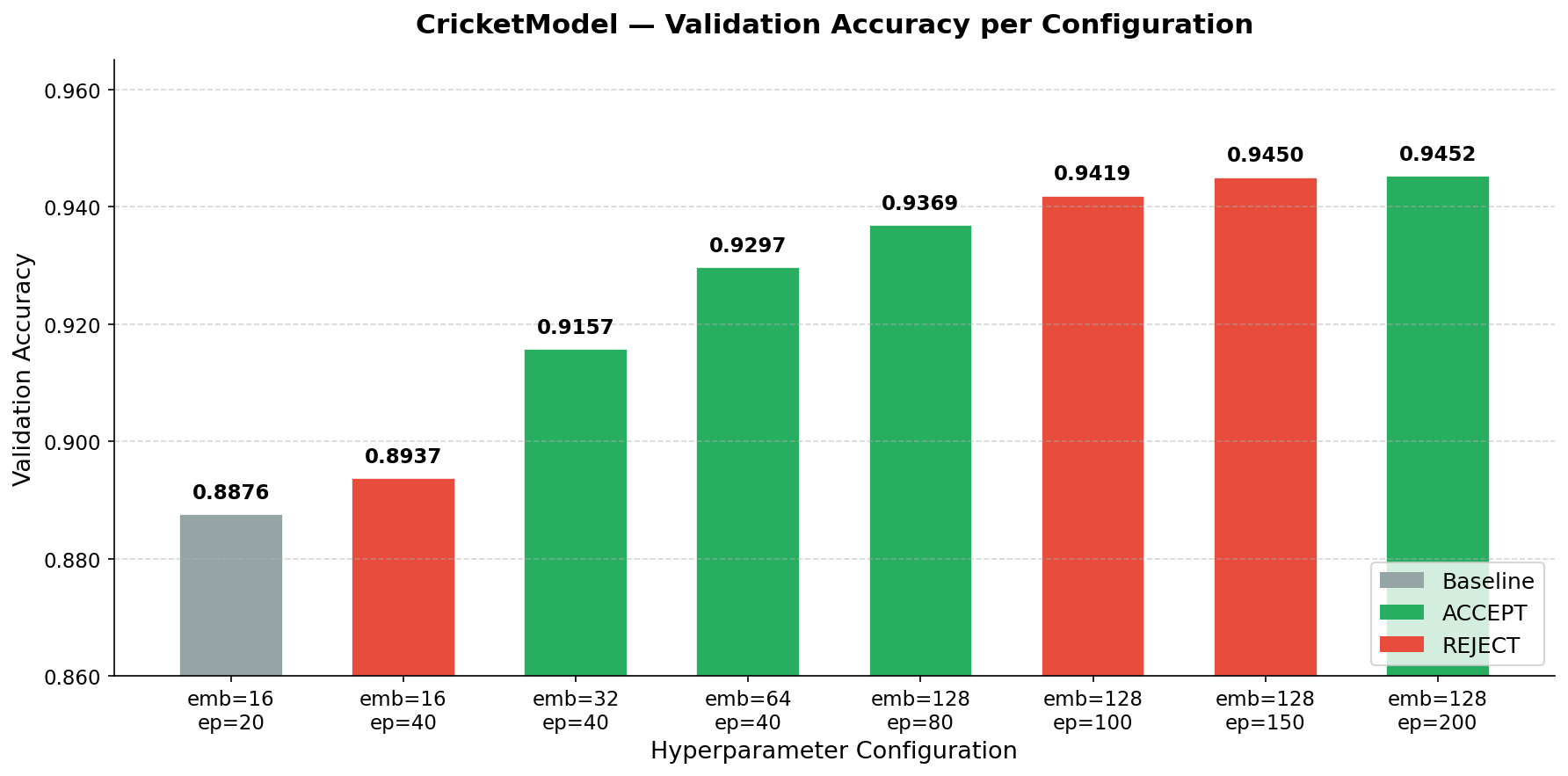
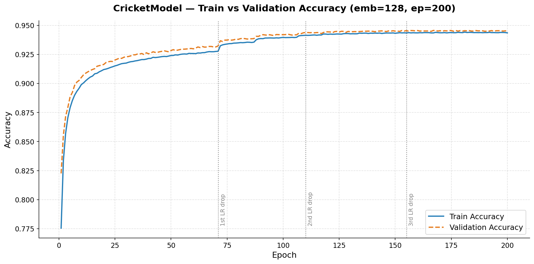
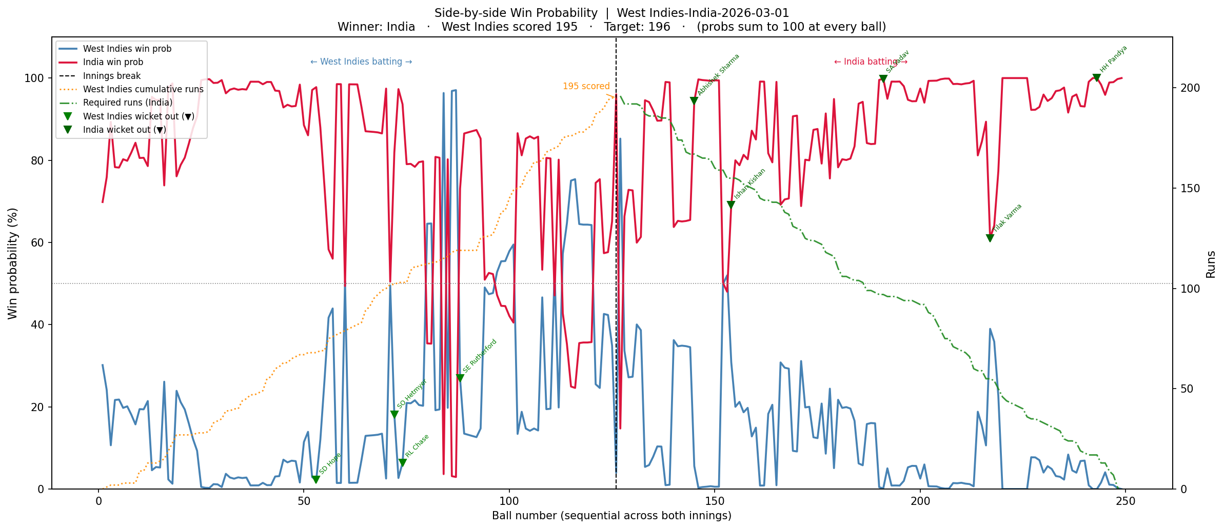
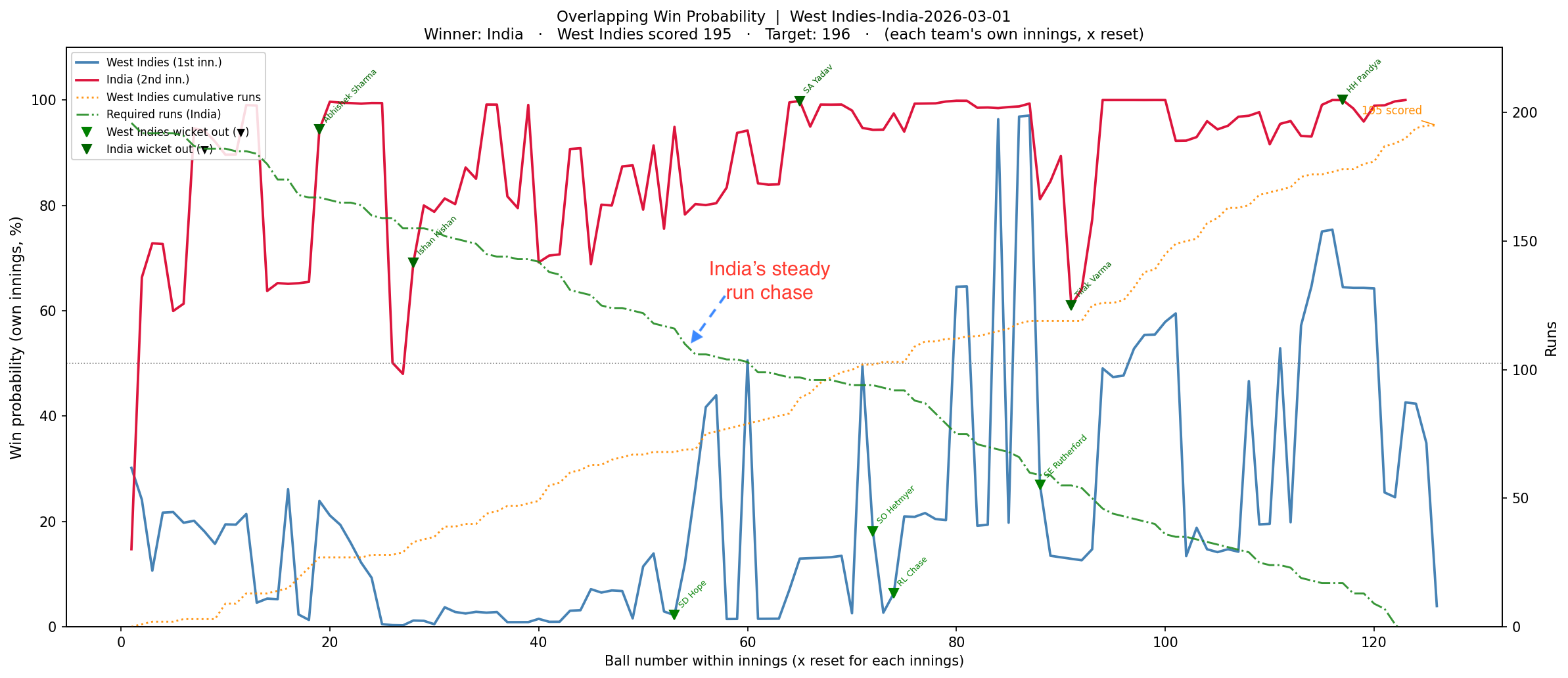
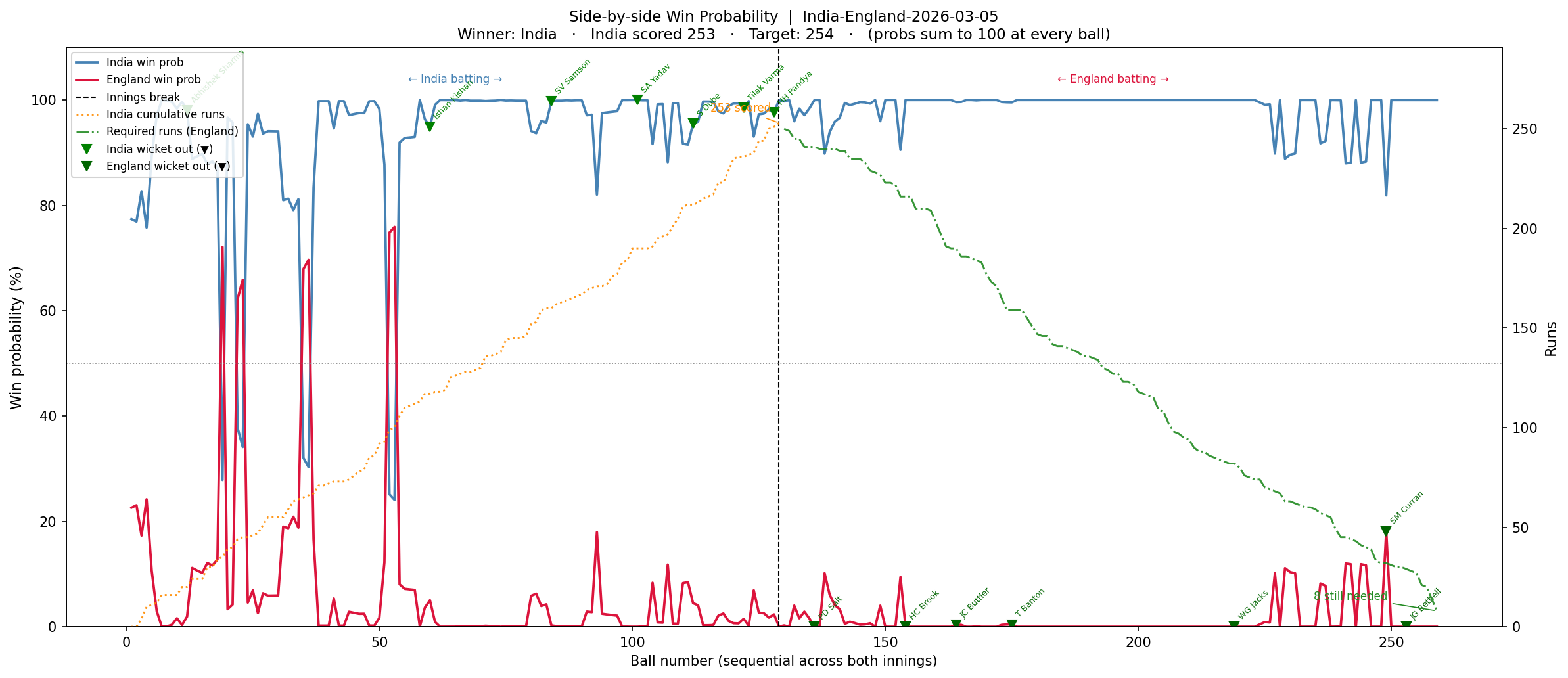
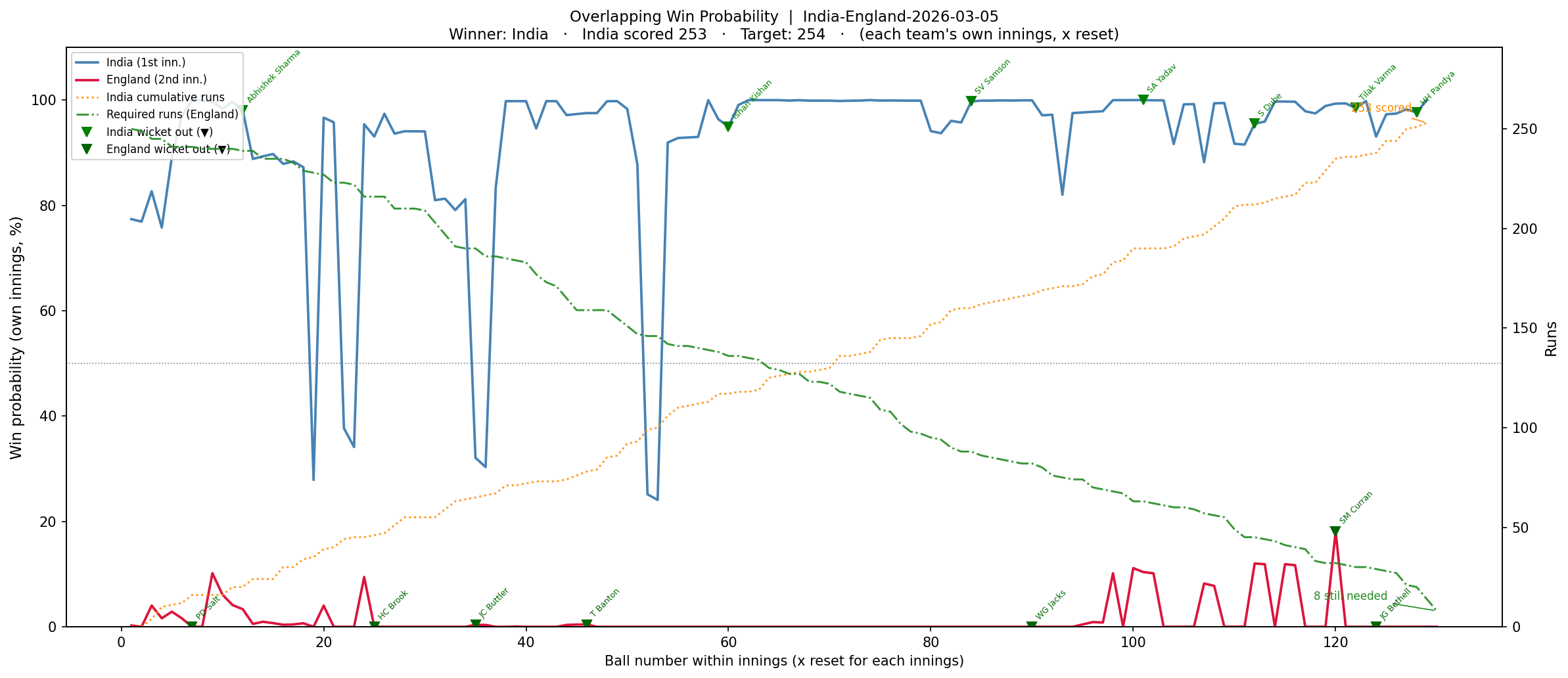
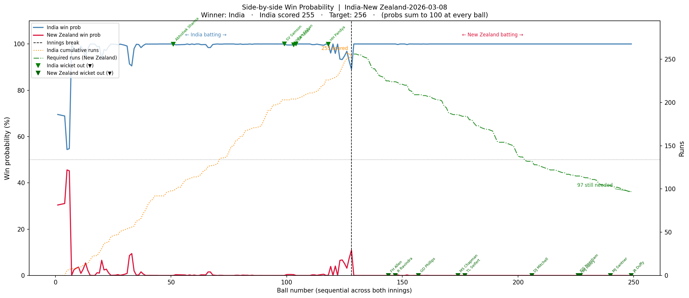
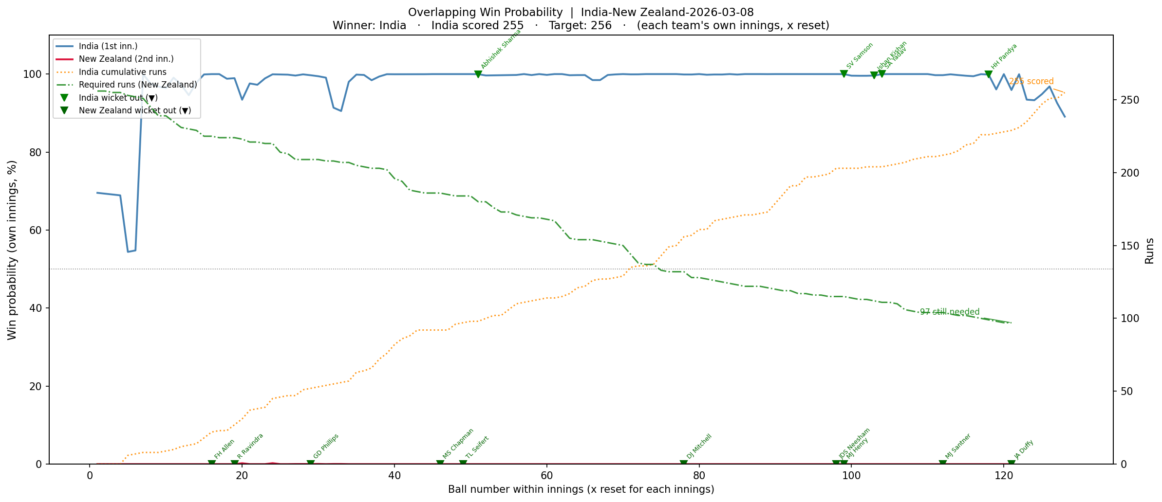

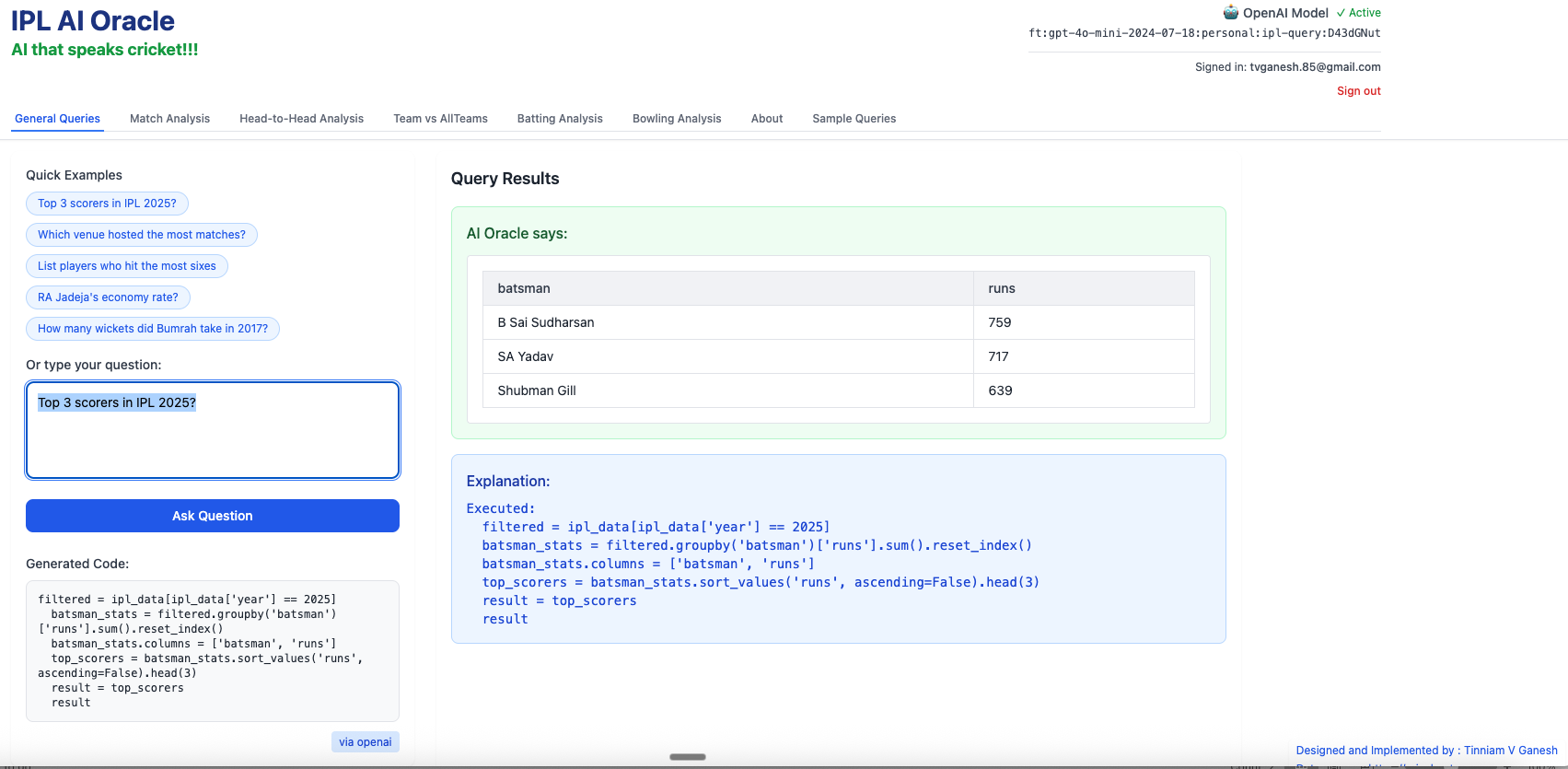
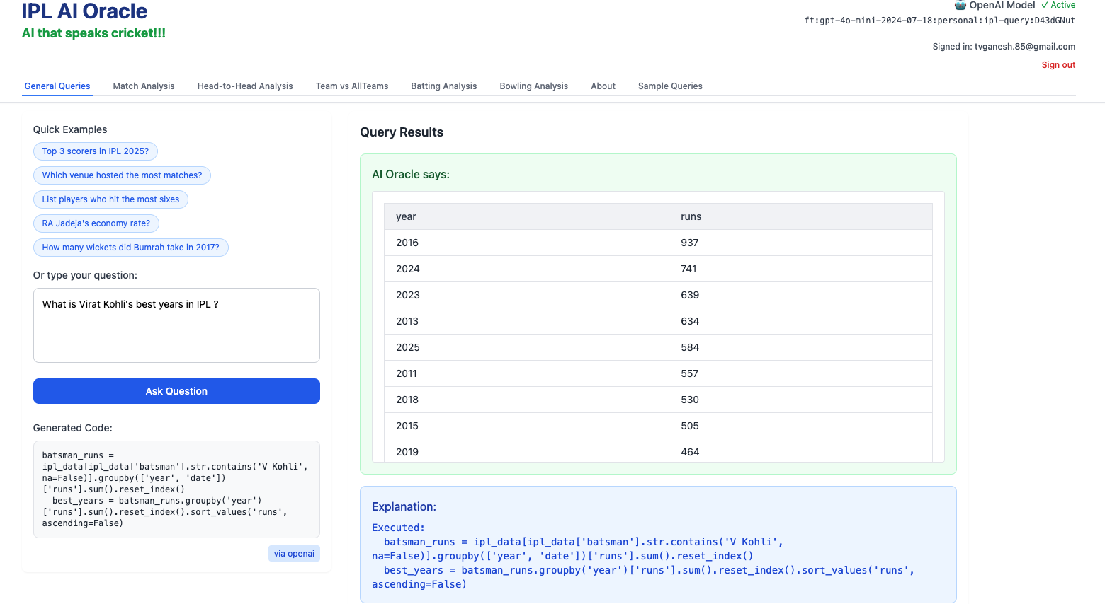
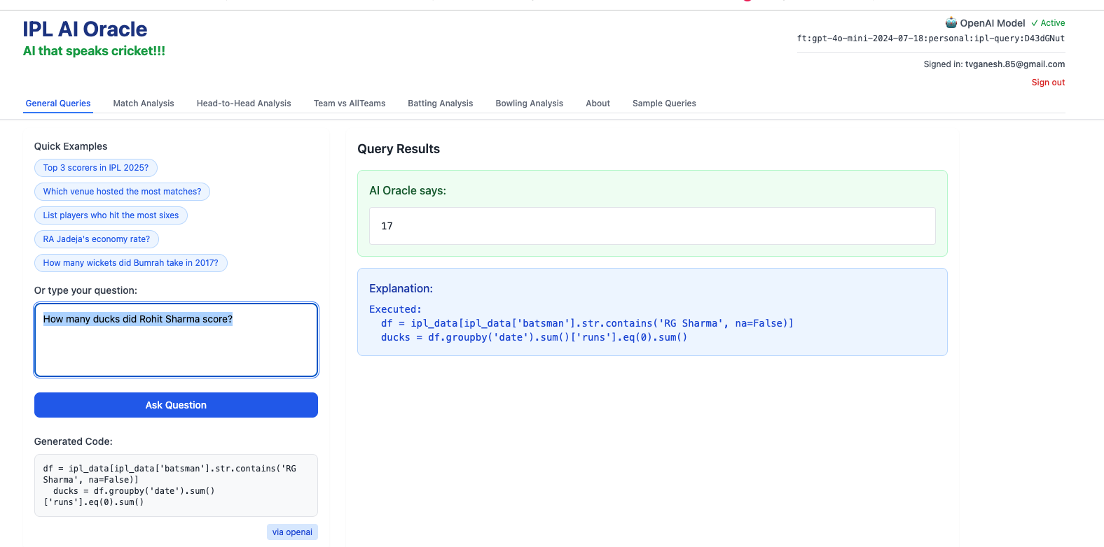
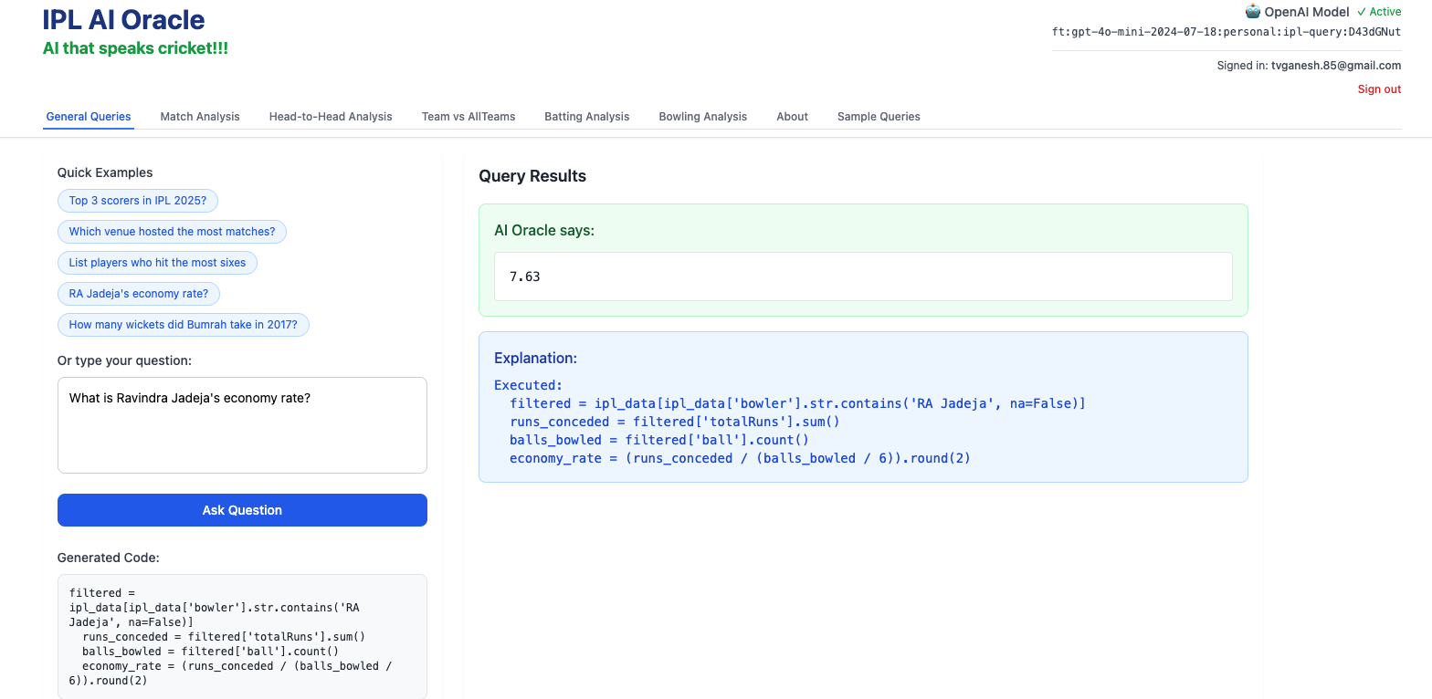
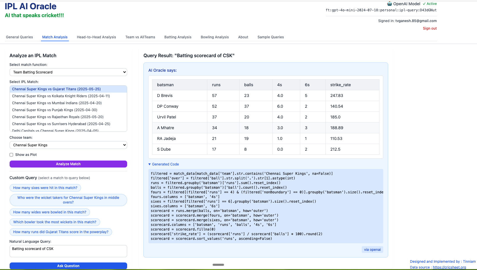
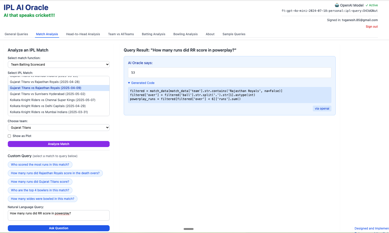
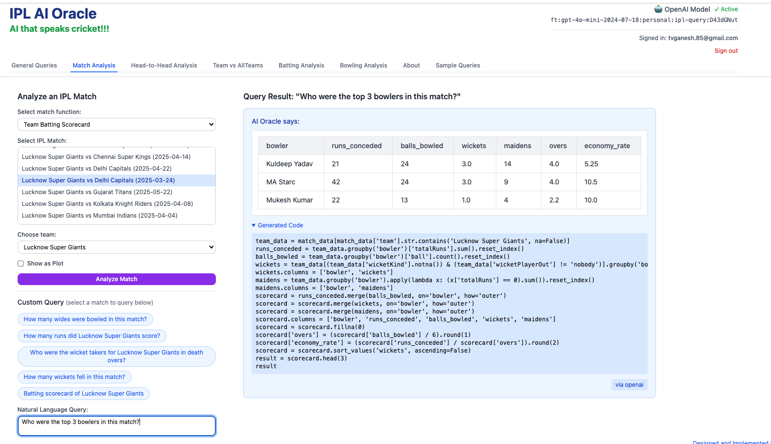
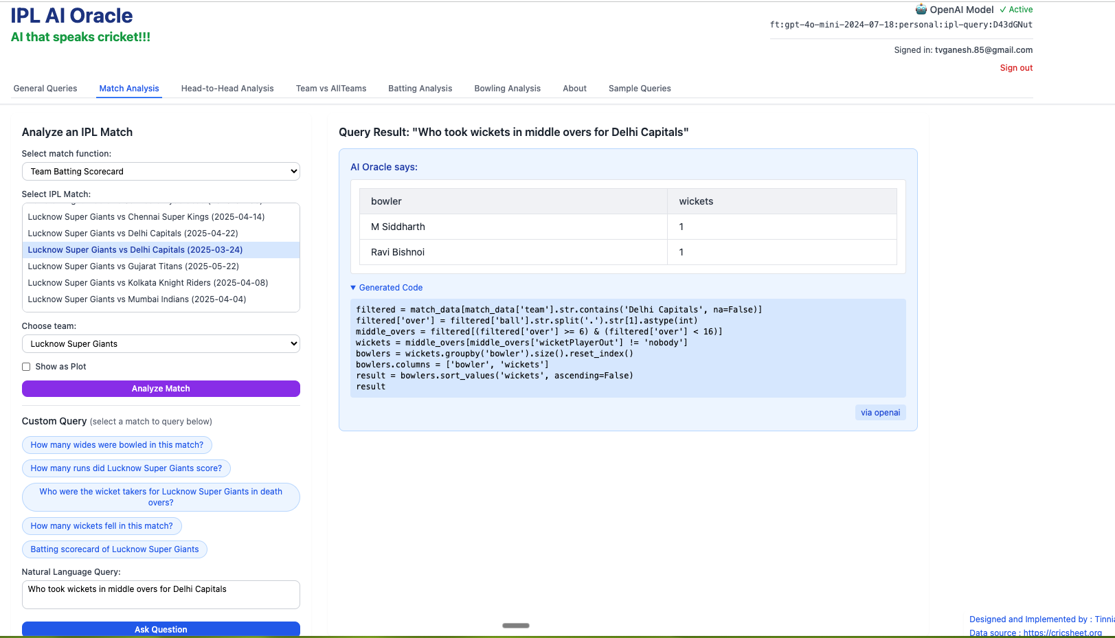
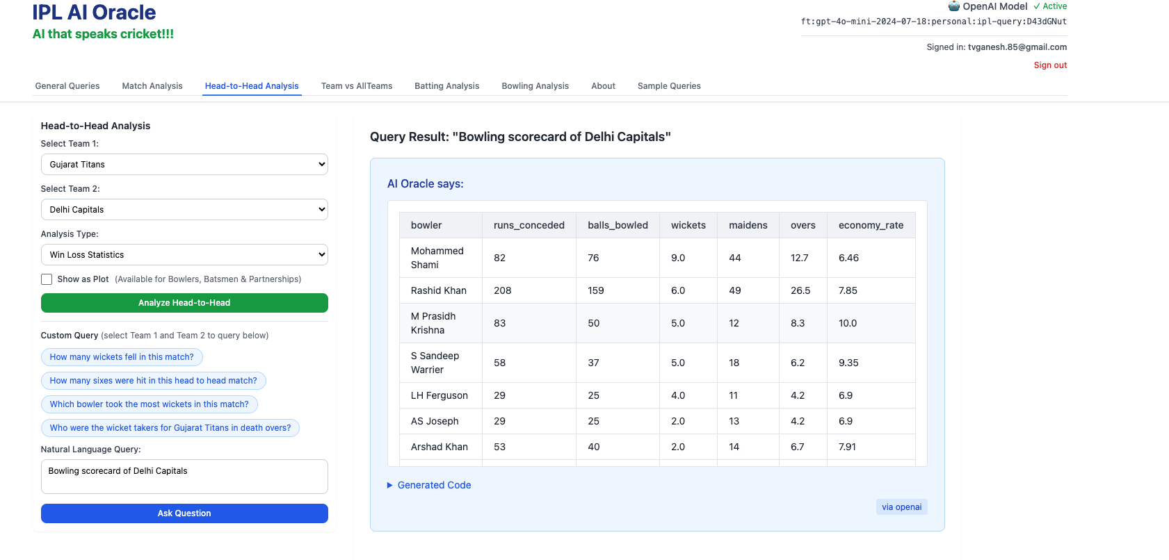
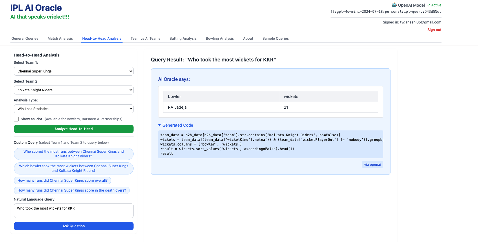
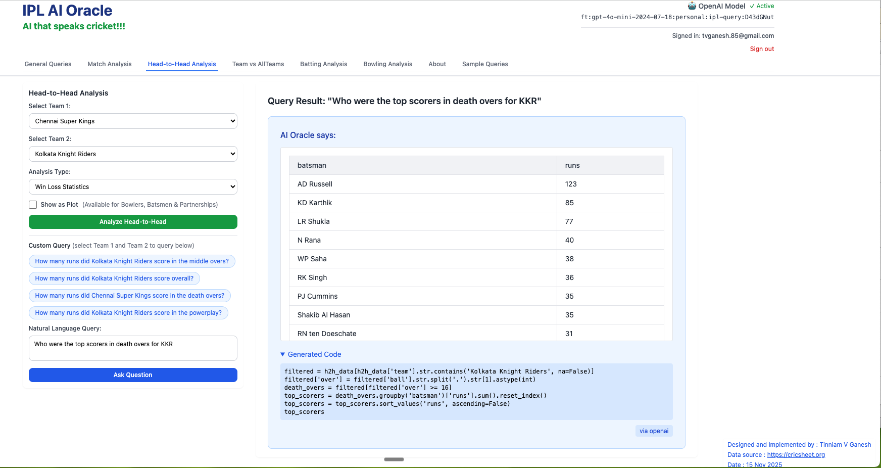
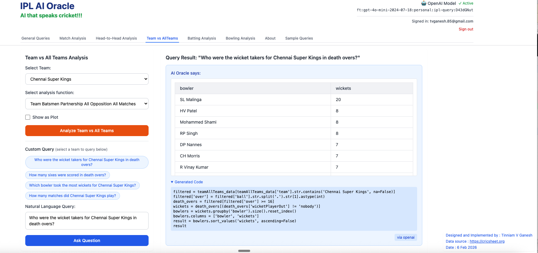
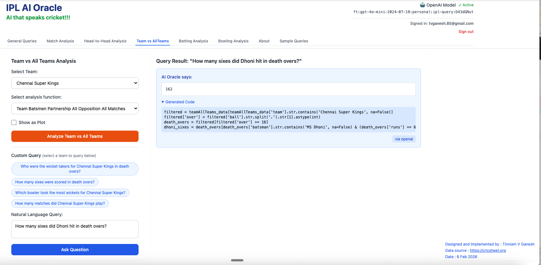
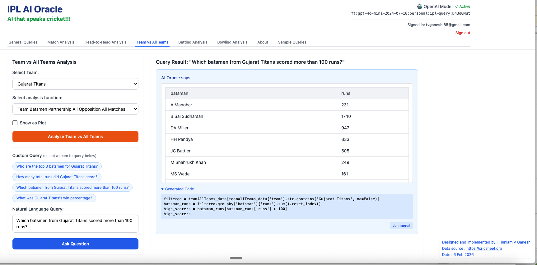
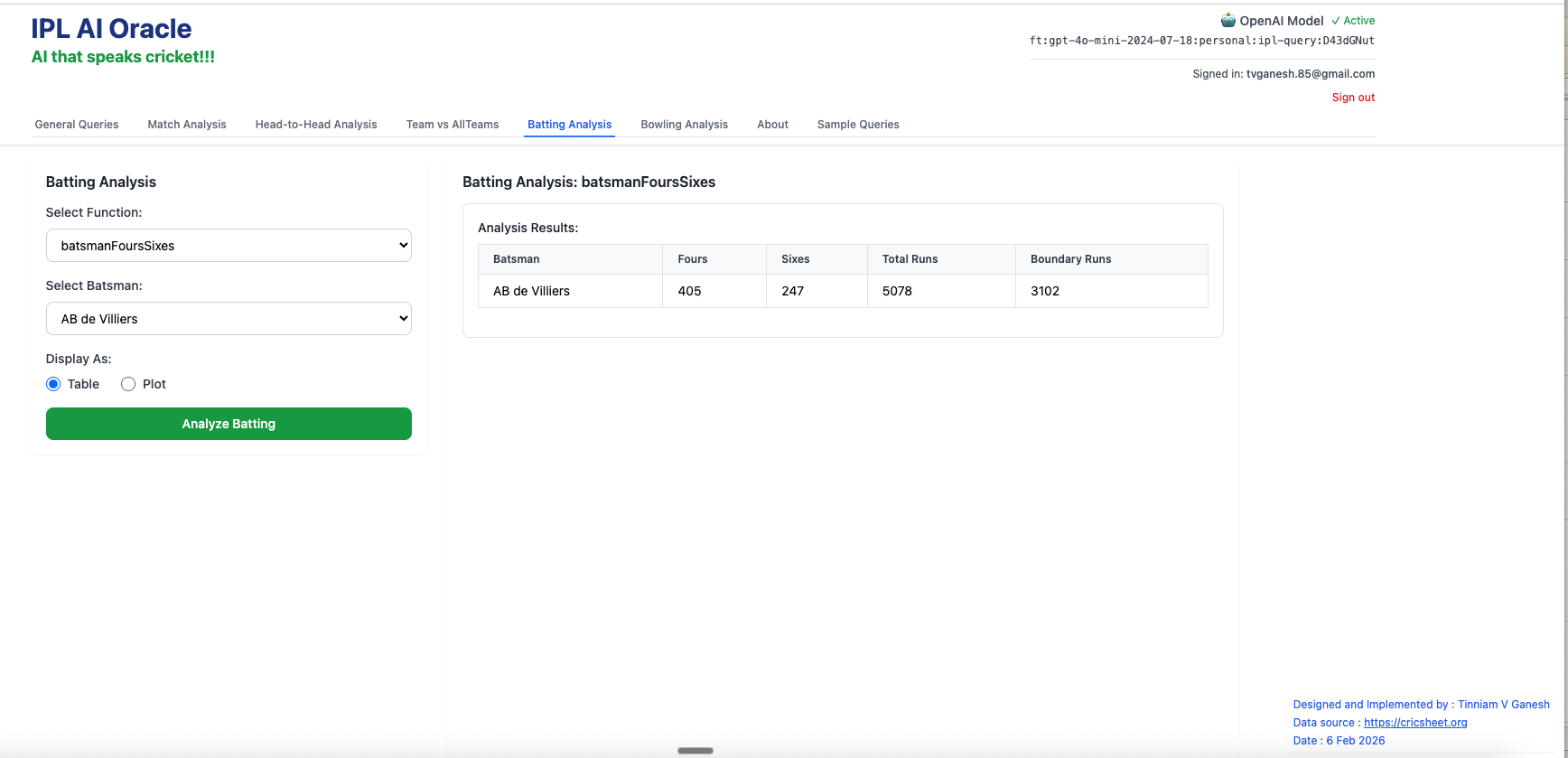
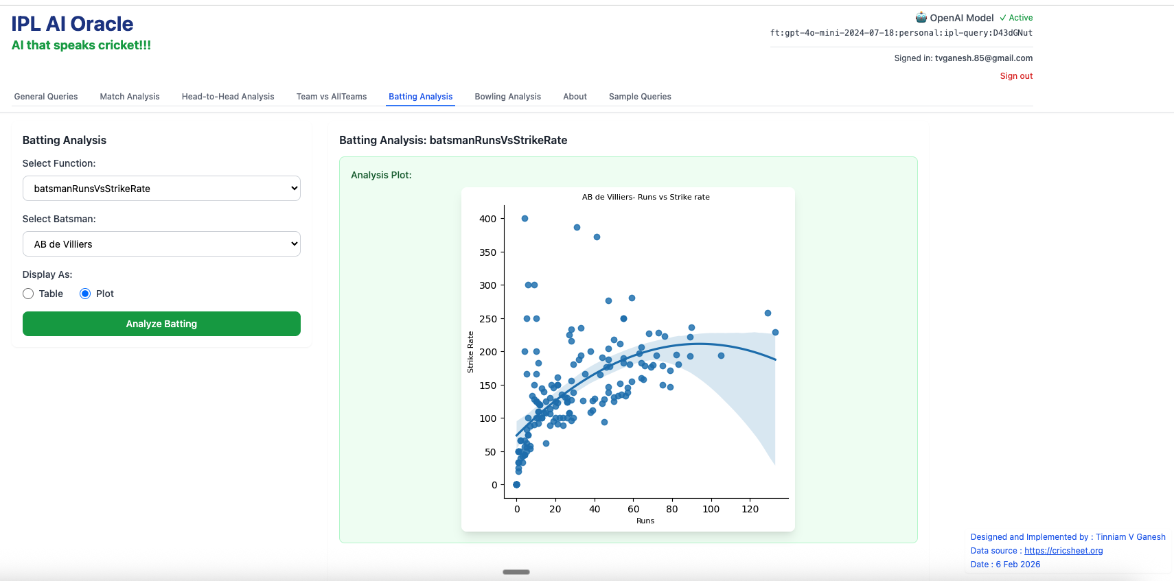
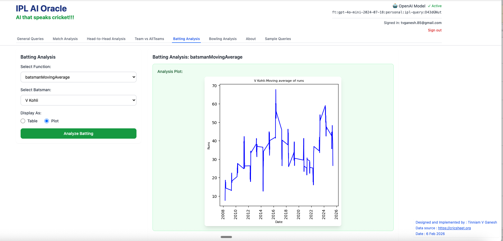
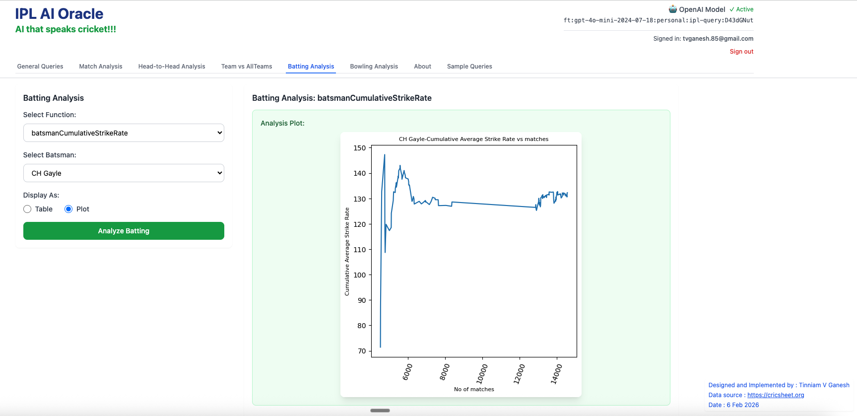
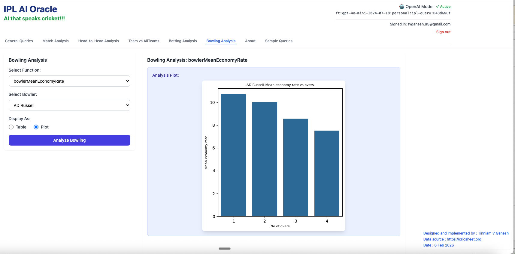
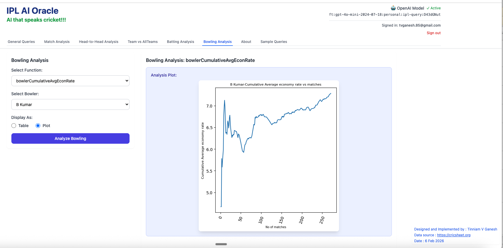
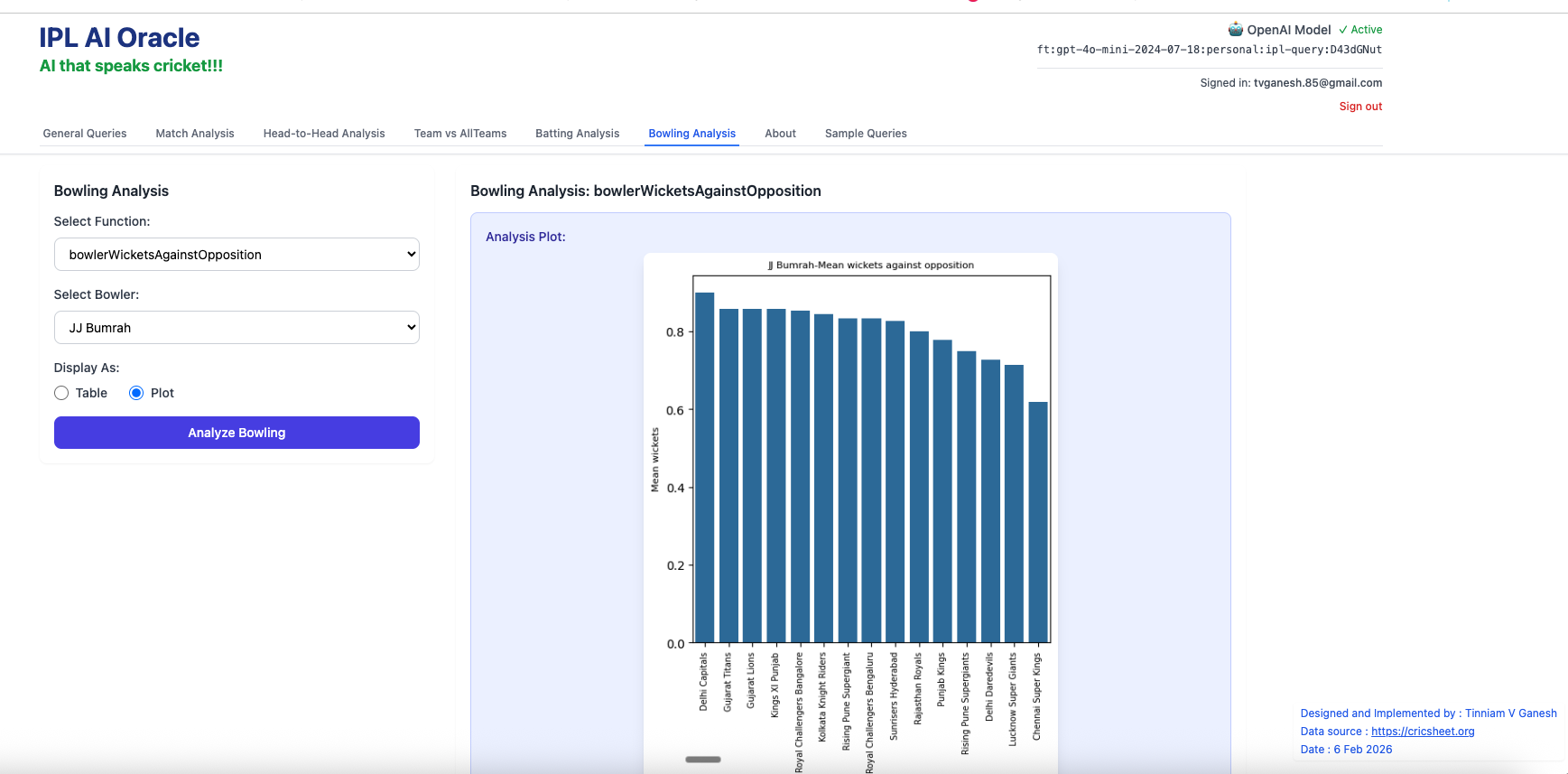


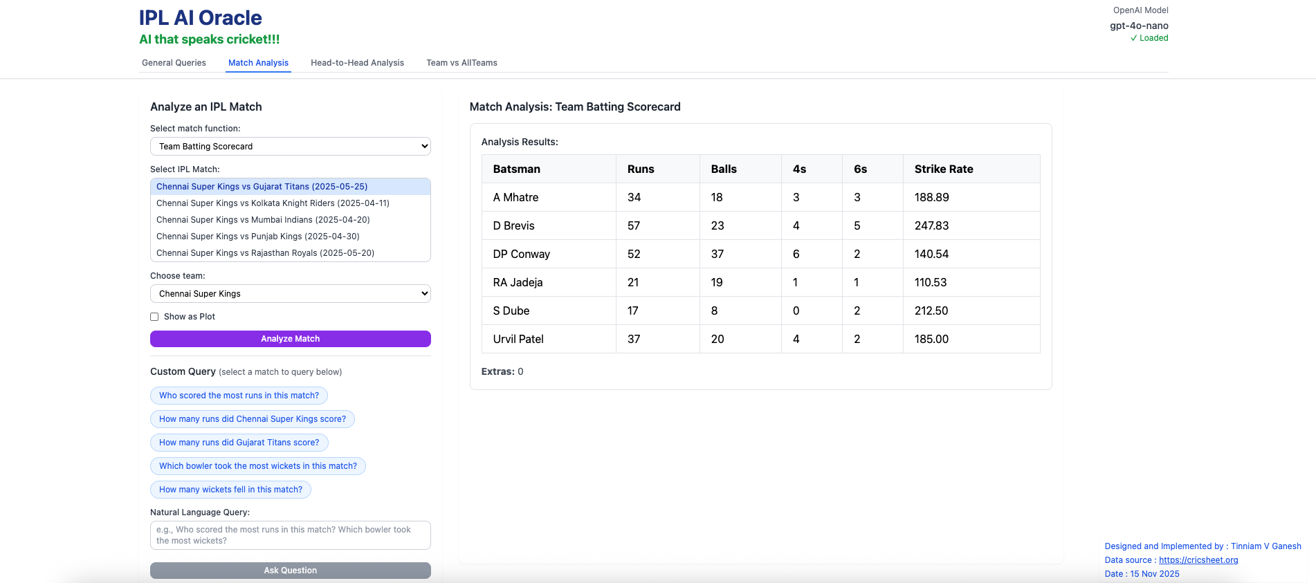
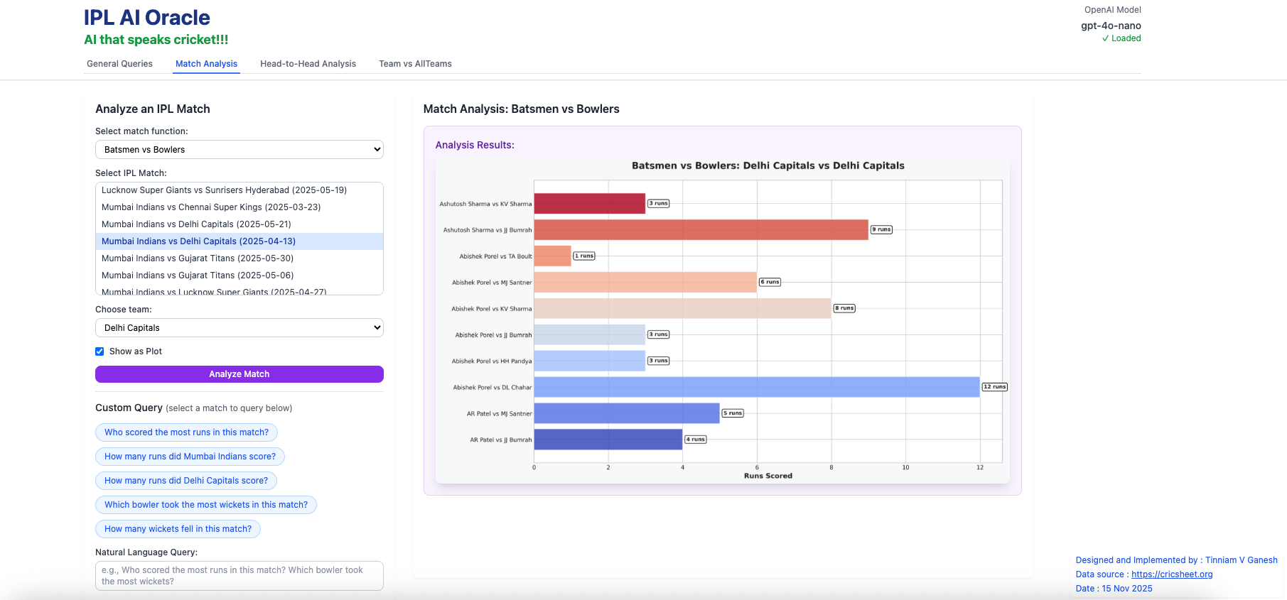
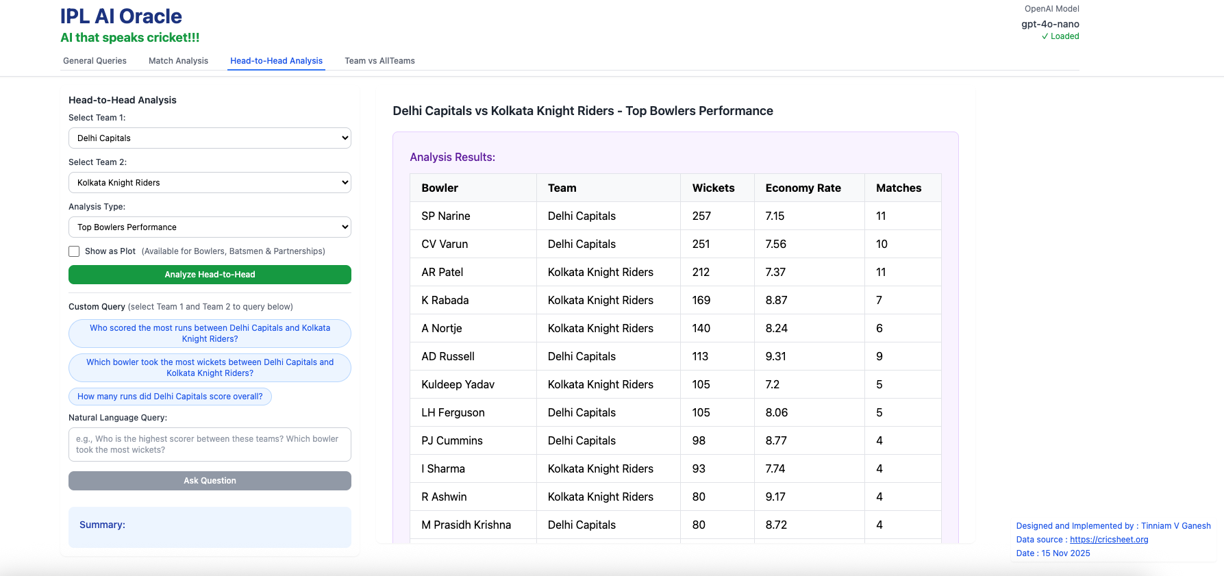
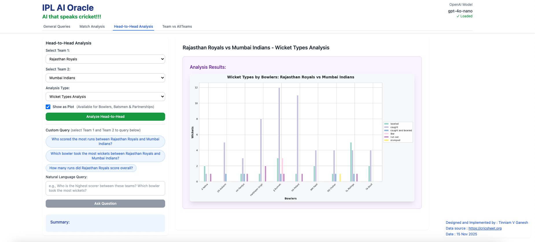
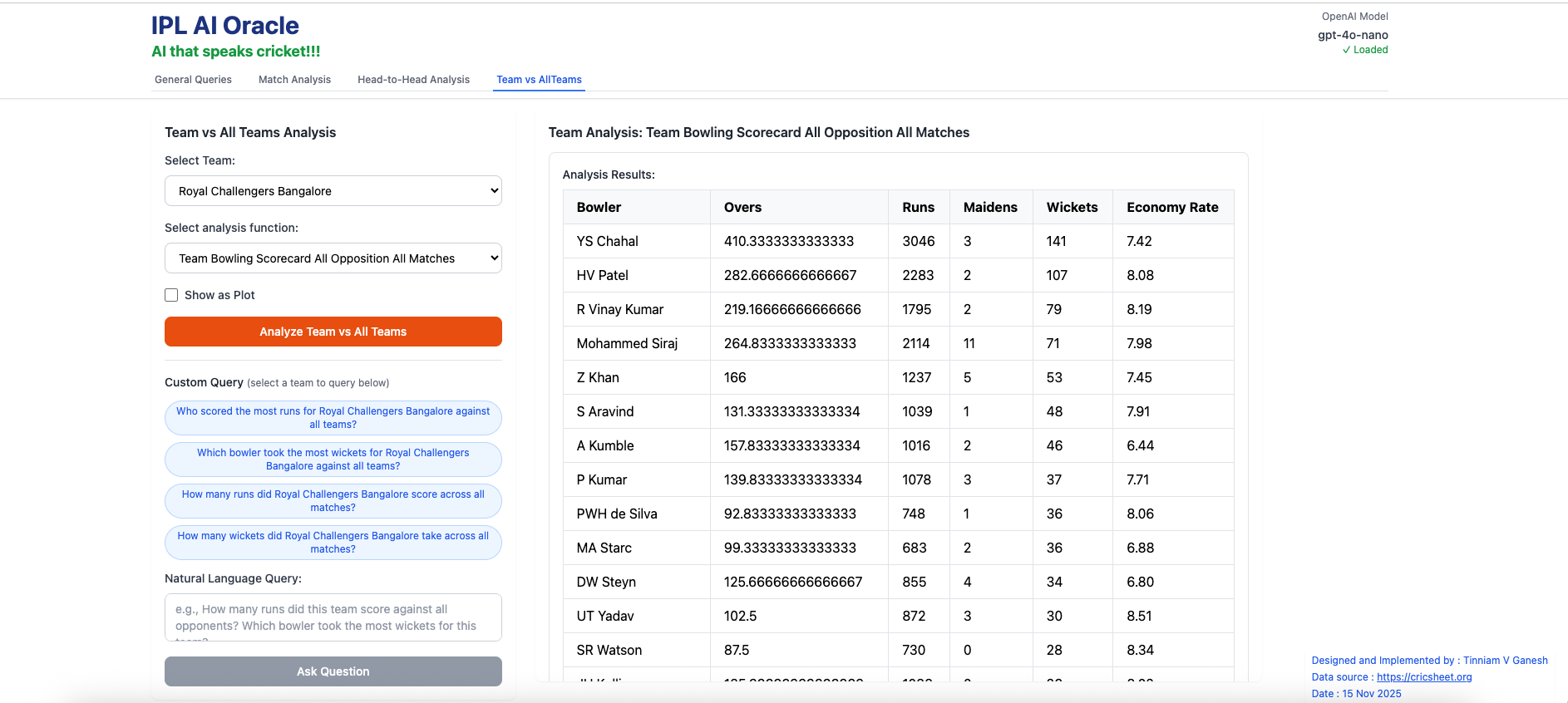
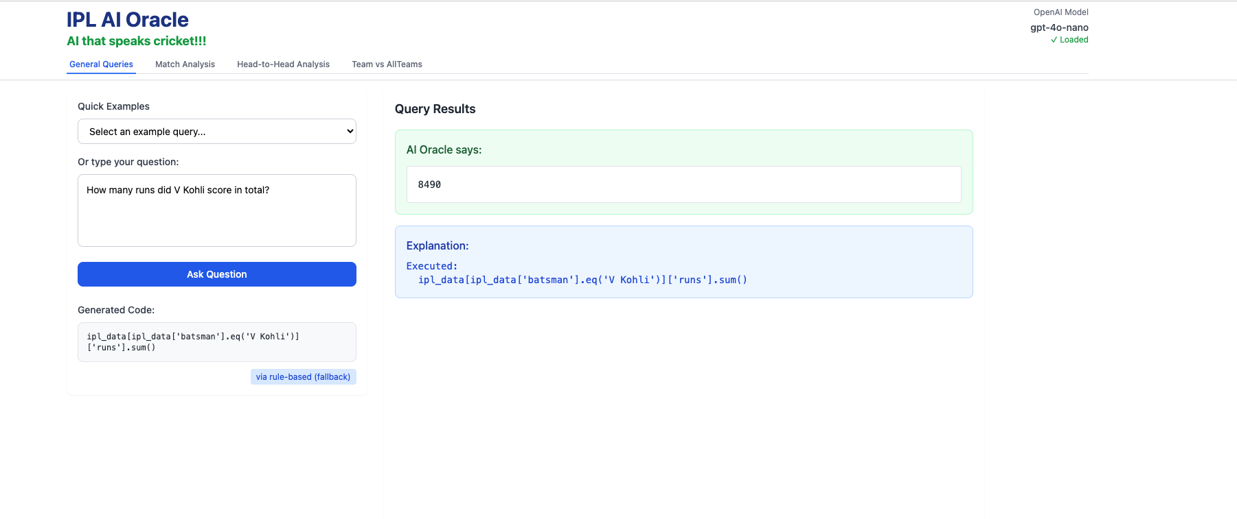
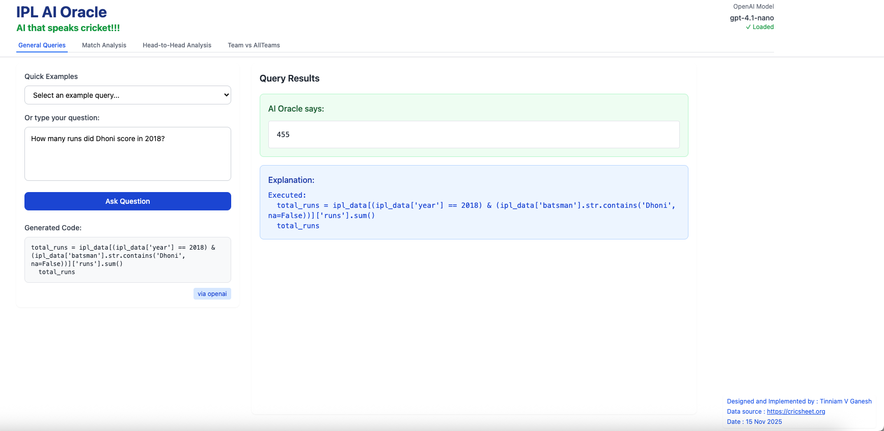
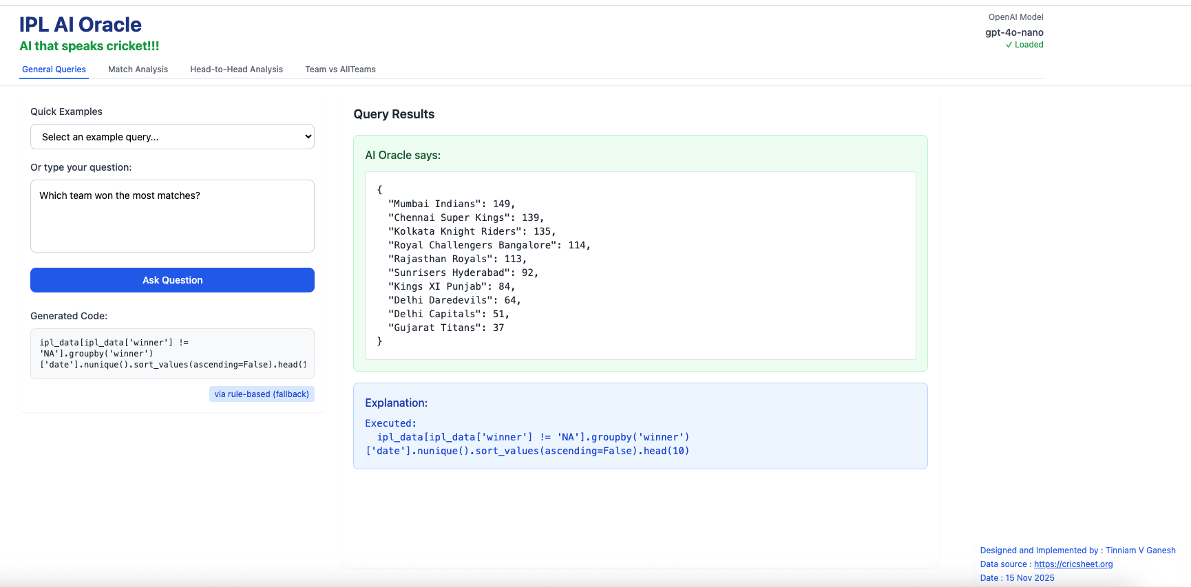
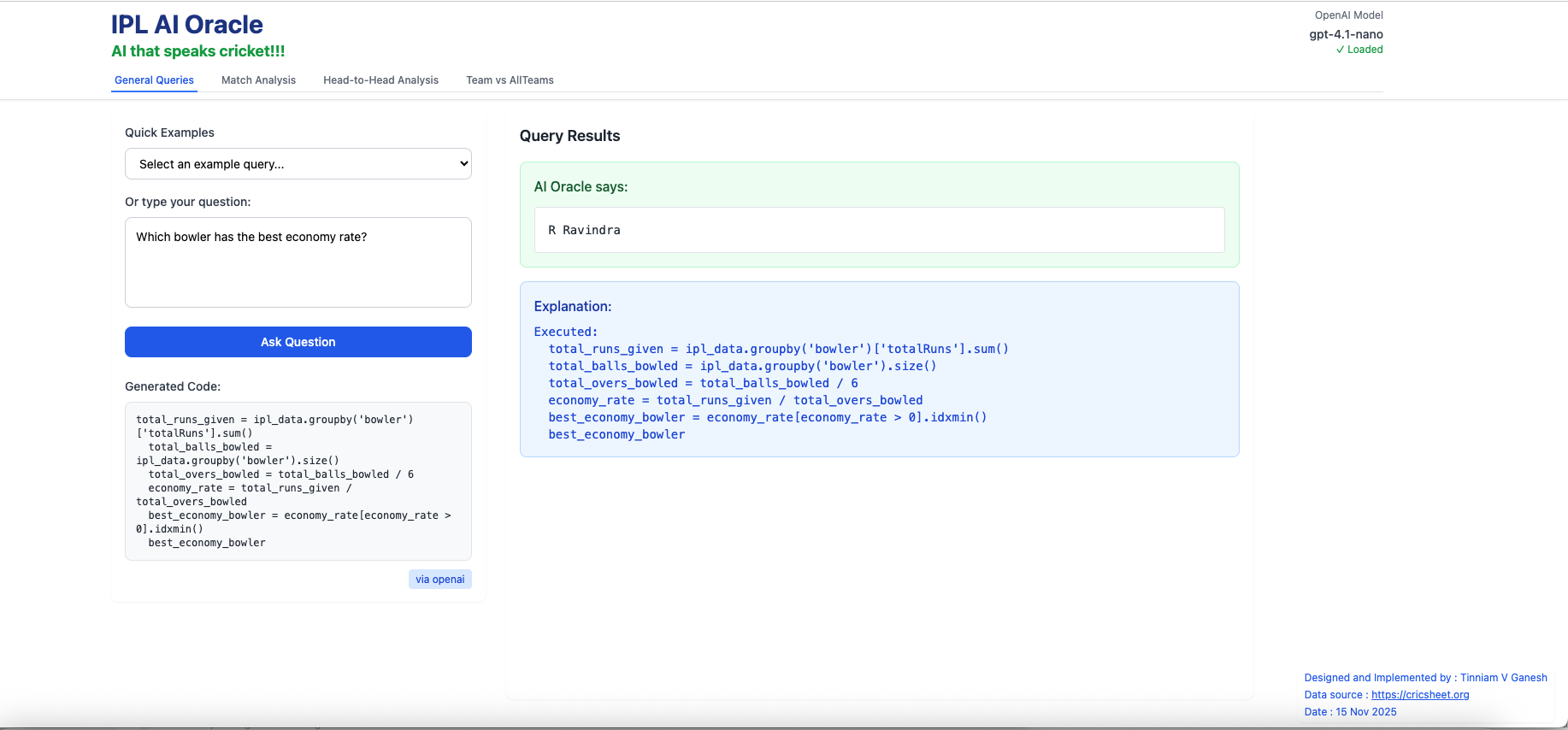
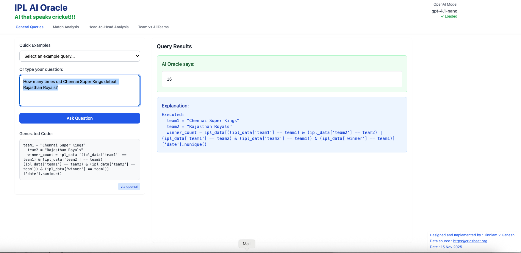
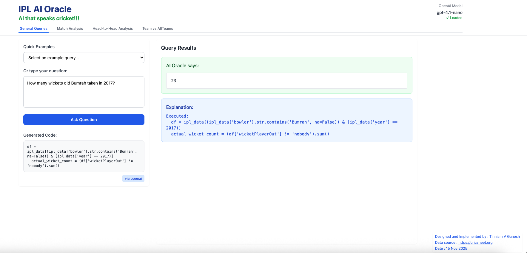
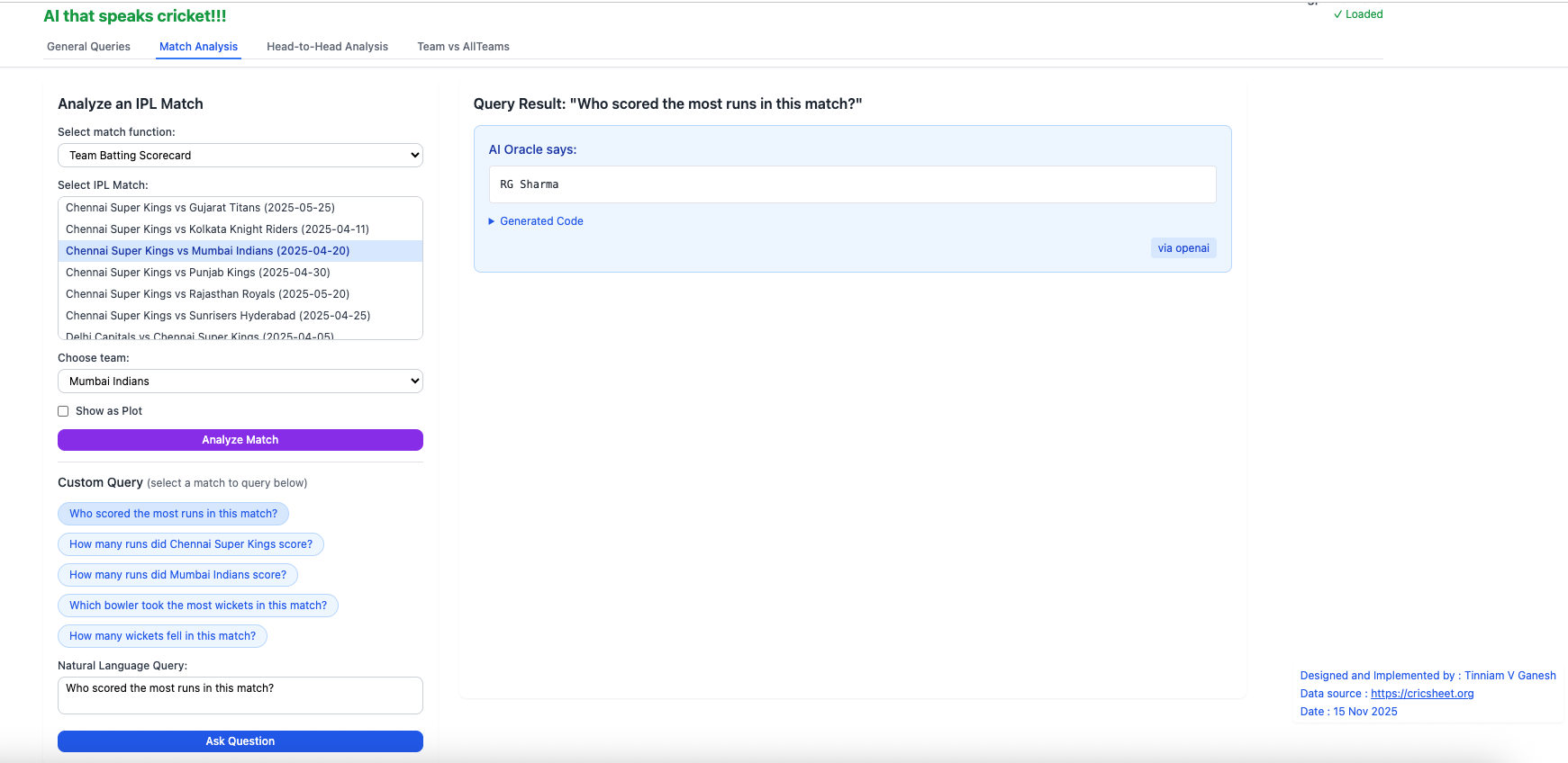
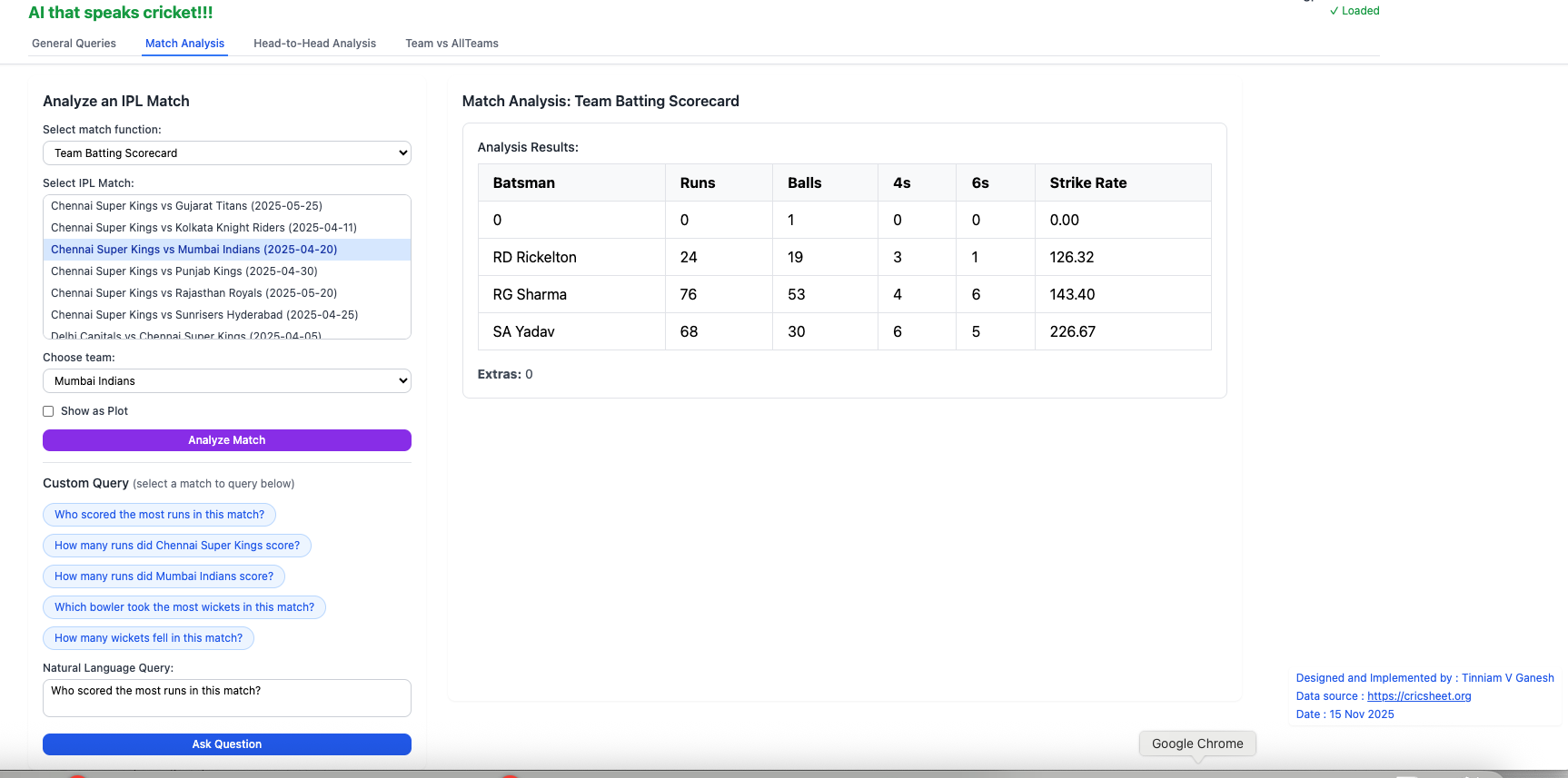
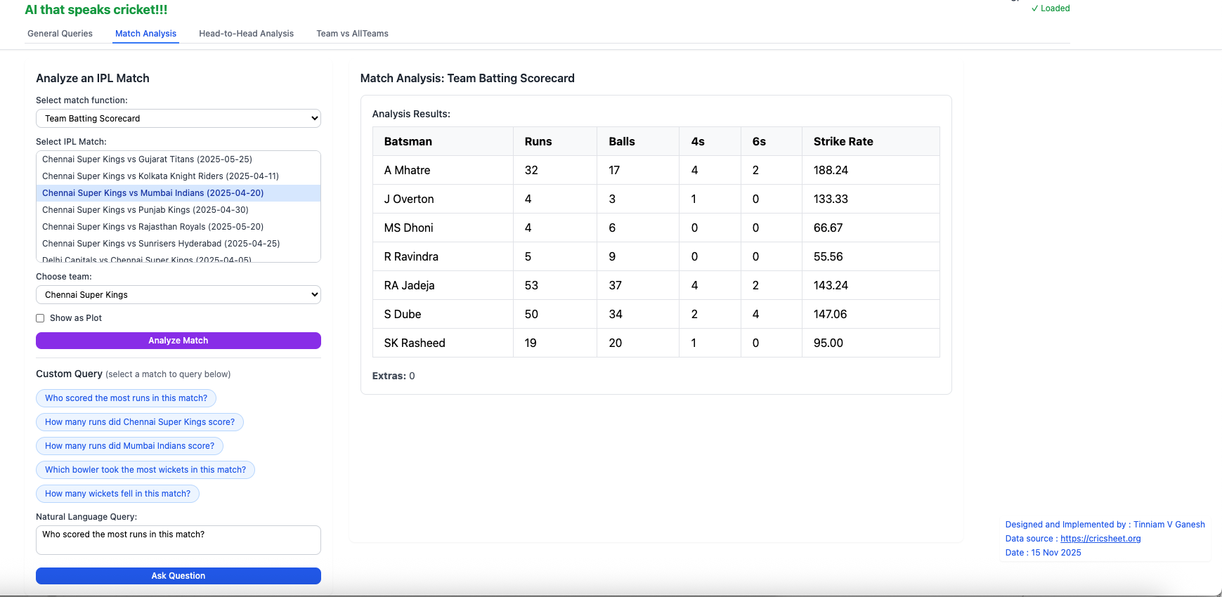
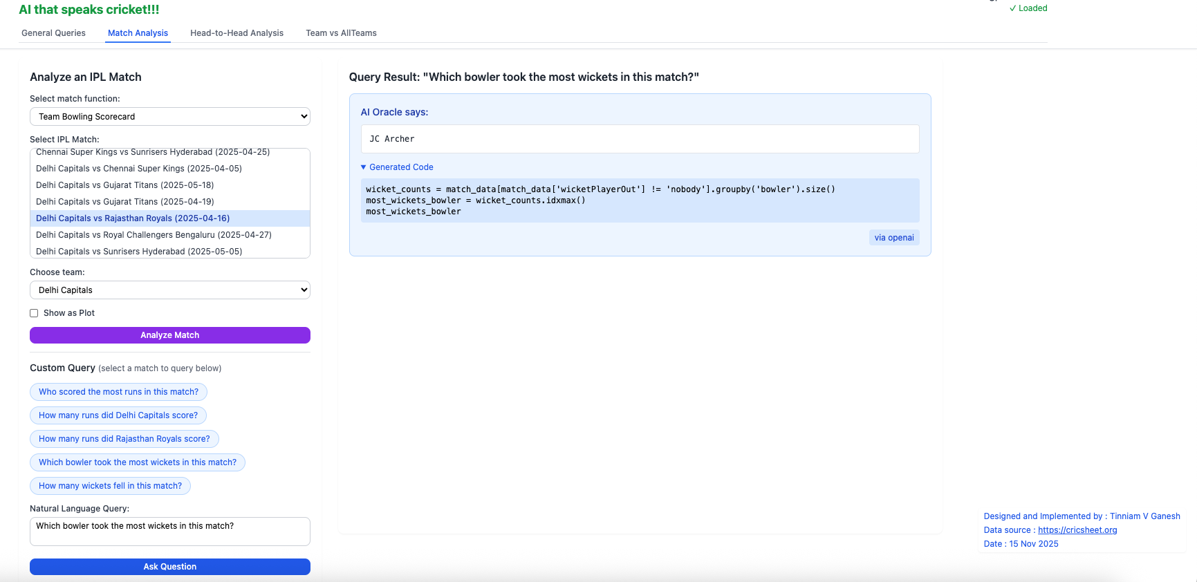
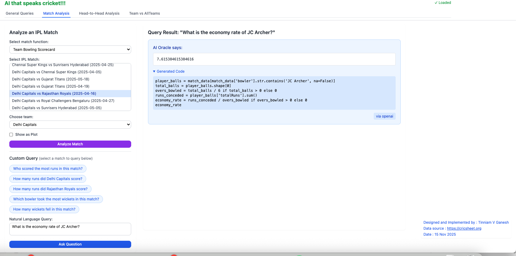
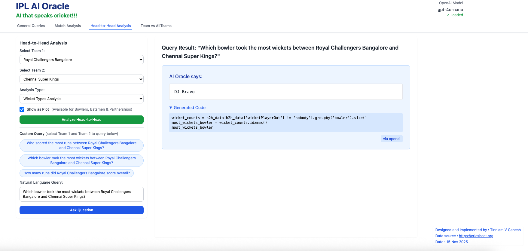
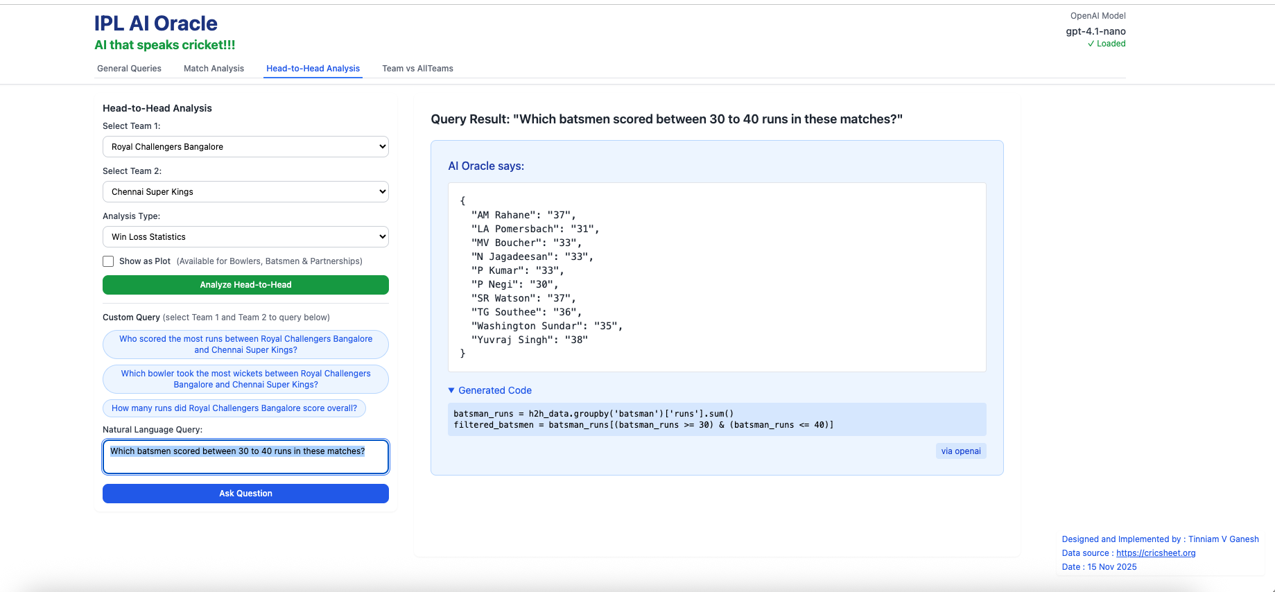
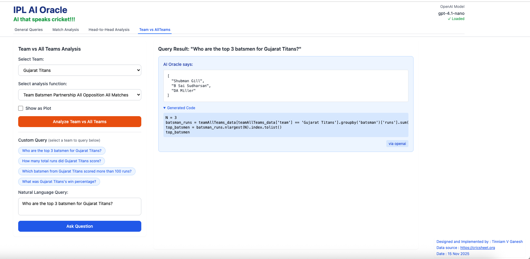
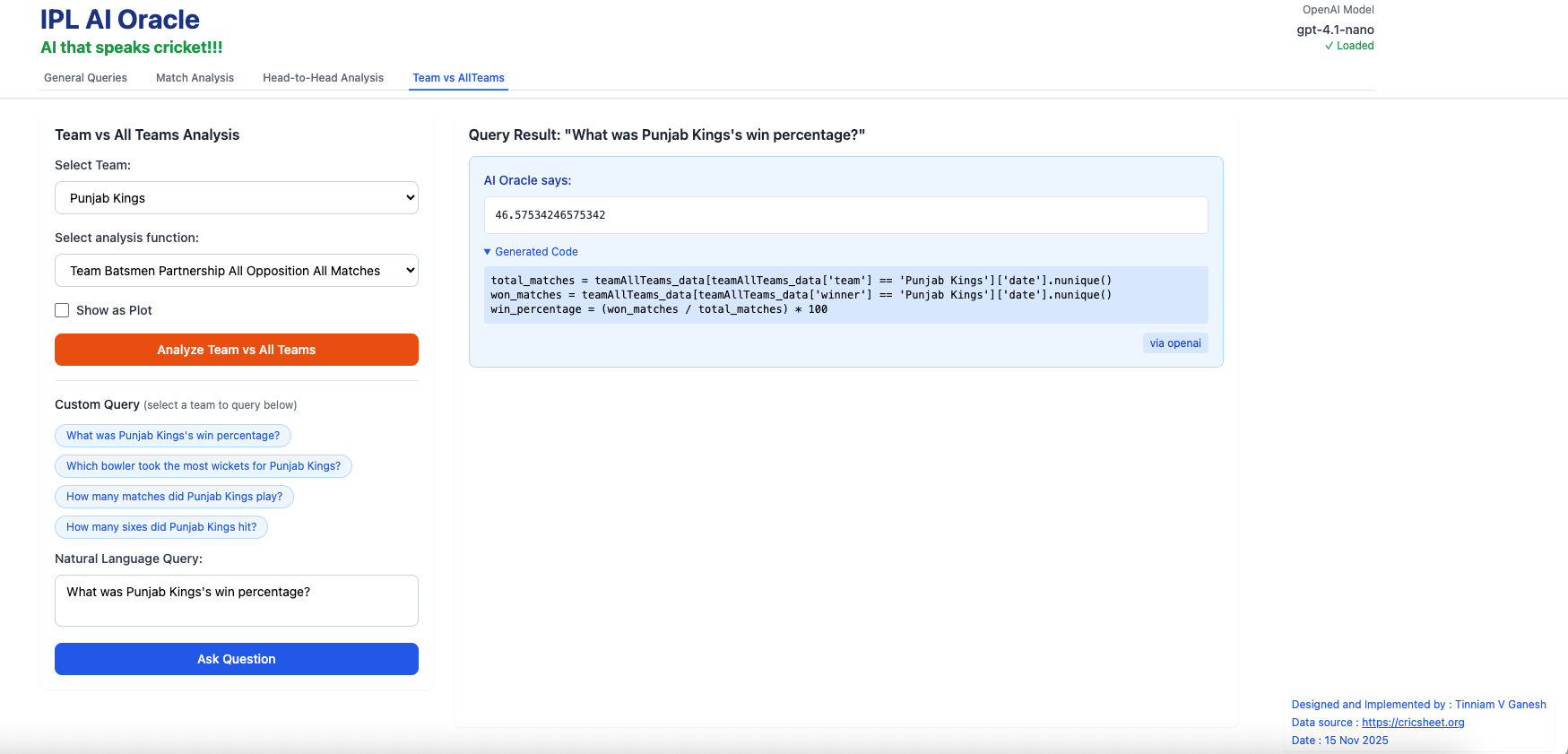


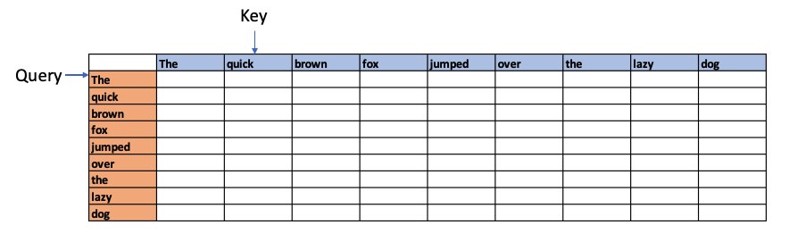
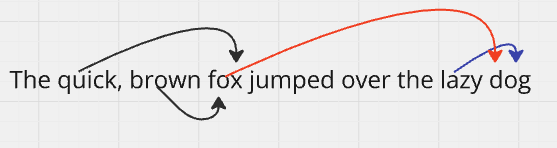
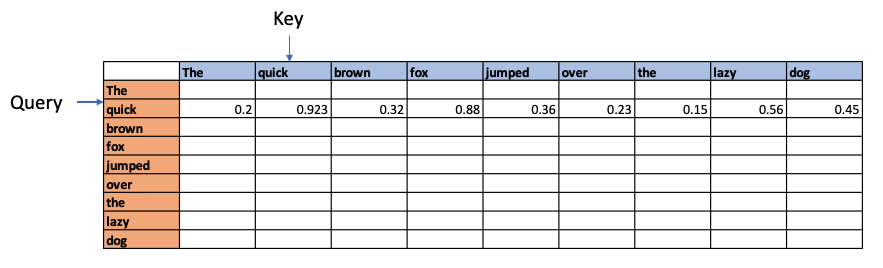
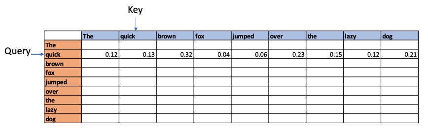

 scales the dot product so that the dot product values are not overly large


 and
and  are the weight matrices, and
  and
and  are the biases
  x
x  and
and x
x  and
and  is the activation function which can be ReLU, GELU or SwiGLU

 ,
,  ,
,  . By multiplyting these matrices with the input vectors we get Q,K and V vectors. The attention is computed as


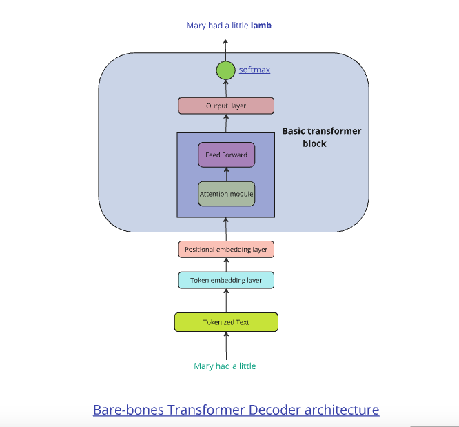
 ,
, 


 = 64
= 64