Analyzing World Bank data with WDI, googleVis Motion Charts

Recently I was surfing the web, when I came across a real cool post New R package to access World Bank data, by Markus Gesmann on using googleVis and motion charts with World Bank Data. The post also introduced me to Hans Rosling, Professor of Sweden’s Karolinska Institute. Hans Rosling, the creator of the famous Gapminder chart, the “Heath and Wealth of Nations” displays global trends through animated charts (A must see!!!). As they say, in Hans Rosling’s hands, data dances and sings. Take a look at some of his Ted talks for e.g. Hans Rosling:New insights on poverty. Prof Rosling developed the breakthrough software behind the visualizations, in the Gapminder. The free software, which can be loaded with any data – was purchased by Google in March 2007.

In this post, I recreate some of the Gapminder charts with the help of R packages WDI and googleVis. The WDI  package of  Vincent Arel-Bundock, provides a set of really useful functions to get to data based on the World Bank Data indicators.  googleVis provides motion charts with which you can animate the data.. Incidentally Datacamp has a very nice, short course on googleVis “Having fun with googleVis

See an updated version of this post Revisiting World Bank data analysis with WDI and gVisMotionChart

You can clone/download the code from Github at worldBankAnalysis which is in the form of an Rmd file.

library(WDI)
library(ggplot2)
library(googleVis)
library(plyr)

1.Get the data from 1960 to 2016 for the following

  1. Population – SP.POP.TOTL
  2. GDP in US $ – NY.GDP.MKTP.CD
  3. Life Expectancy at birth (Years) – SP.DYN.LE00.IN
  4. GDP Per capita income – NY.GDP.PCAP.PP.CD
  5. Fertility rate (Births per woman) – SP.DYN.TFRT.IN
  6. Poverty headcount ratio – SI.POV.2DAY
# World population total
population = WDI(indicator='SP.POP.TOTL', country="all",start=1960, end=2016)
# GDP in US $
gdp= WDI(indicator='NY.GDP.MKTP.CD', country="all",start=1960, end=2016)
# Life expectancy at birth (Years)
lifeExpectancy= WDI(indicator='SP.DYN.LE00.IN', country="all",start=1960, end=2016)
# GDP Per capita
income = WDI(indicator='NY.GDP.PCAP.PP.CD', country="all",start=1960, end=2016)
# Fertility rate (births per woman)
fertility = WDI(indicator='SP.DYN.TFRT.IN', country="all",start=1960, end=2016)
# Poverty head count
poverty= WDI(indicator='SI.POV.2DAY', country="all",start=1960, end=2016)

2.Rename the columns

names(population)[3]="Total population"
names(lifeExpectancy)[3]="Life Expectancy (Years)"
names(gdp)[3]="GDP (US$)"
names(income)[3]="GDP per capita income"
names(fertility)[3]="Fertility (Births per woman)"
names(poverty)[3]="Poverty headcount ratio"

3.Join the data frames

Join the individual data frames to one large wide data frame with all the indicators for the countries


j1 <- join(population, gdp)
j2 <- join(j1,lifeExpectancy)
j3 <- join(j2,income)
j4 <- join(j3,poverty)
wbData <- join(j4,fertility)

4.Use WDI_data

Use WDI_data to get the list of indicators and the countries. Join the countries and region

#This returns  list of 2 matrixes
wdi_data =WDI_data
# The 1st matrix is the list is the set of all World Bank Indicators
indicators=wdi_data[[1]]
# The 2nd  matrix gives the set of countries and regions
countries=wdi_data[[2]]
df = as.data.frame(countries)
aa <- df$region != "Aggregates"
# Remove the aggregates
countries_df <- df[aa,]
# Subset from the development data only those corresponding to the countries
bb = subset(wbData, country %in% countries_df$country)
cc = join(bb,countries_df)
dd = complete.cases(cc)
developmentDF = cc[dd,]

5.Create and display the motion chart

gg<- gvisMotionChart(cc,
                                idvar = "country",
                                timevar = "year",
                                xvar = "GDP",
                                yvar = "Life Expectancy",
                                sizevar ="Population",
                                colorvar = "region")
plot(gg)
cat(gg$html$chart, file="chart1.html")

Note: Unfortunately it is not possible to embed the motion chart in WordPress. It is has to hosted on a server as a Webpage. After exploring several possibilities I came up with the following process to display the animation graph. The plot is saved as a html file using ‘cat’ as shown above. The chart1.html page is then hosted as a Github page (gh-page) on Github.

Here is the ggvisMotionChart

Do give  World Bank Motion Chart1  a spin.  Here is how the Motion Chart has to be used

untitled

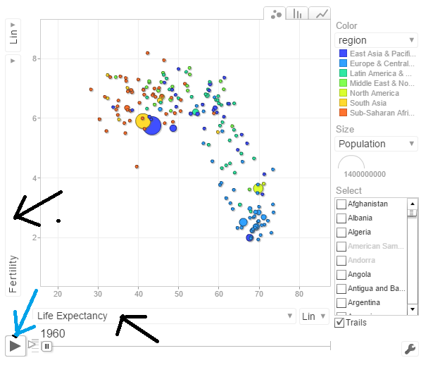
You can select Life Expectancy, Population, Fertility etc by clicking the black arrows. The blue arrow shows the ‘play’ button to set animate the motion chart. You can also select the countries and change the size of the circles. Do give it a try. Here are some quick analysis by playing around with the motion charts with different parameters chosen

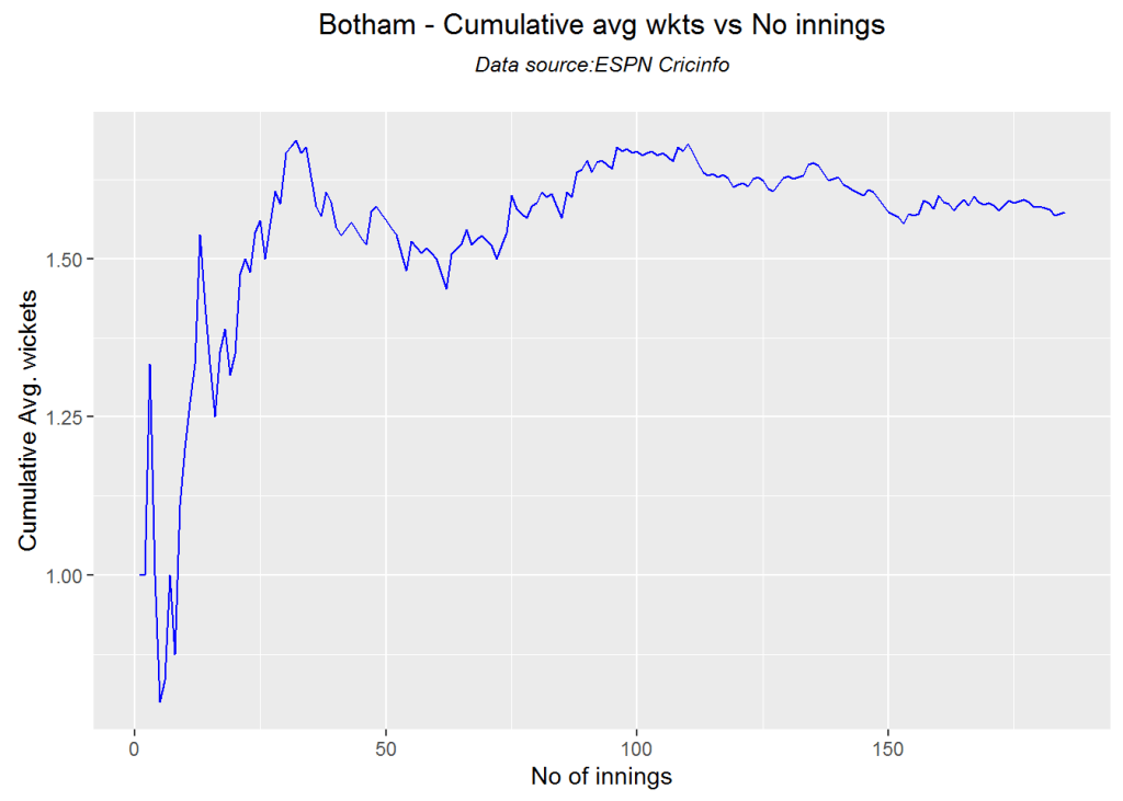
The set of charts below are screenshots captured by running the motion chart World Bank Motion Chart1

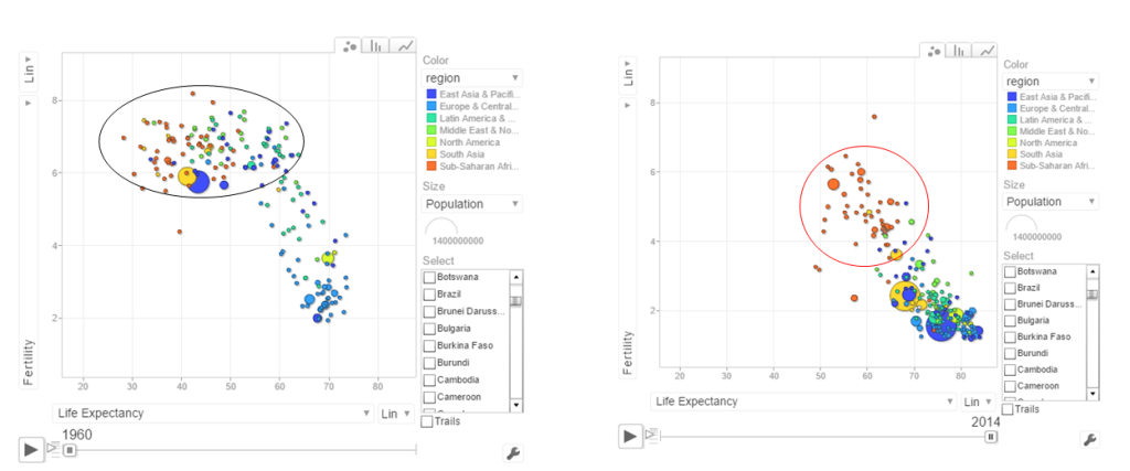
a. Life Expectancy vs Fertility chart

This chart is used by Hans Rosling in his Ted talk. The left chart shows low life expectancy and high fertility rate for several sub Saharan and East Asia Pacific countries in the early 1960’s. Today the fertility has dropped and the life expectancy has increased overall. However the sub Saharan countries still have a high fertility rate

pic1

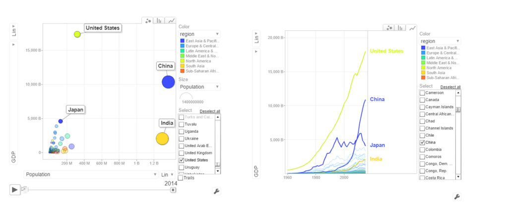
b. Population vs GDP

The chart below shows that GDP of India and China have the same GDP from 1973-1994 with US and Japan well ahead.

pic2

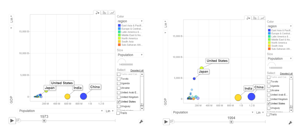
From 1998- 2014 China really pulls away from India and Japan as seen below

pic3

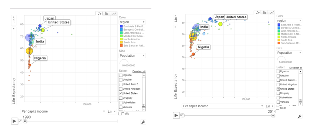
c. Per capita income vs Life Expectancy

In the 1990’s the per capita income and life expectancy of the sub -saharan countries are low (42-50). Japan and US have a good life expectancy in 1990’s. In 2014 the per capita income of the sub-saharan countries are still low though the life expectancy has marginally improved.

pic4

d. Population vs Poverty headcount

pic5

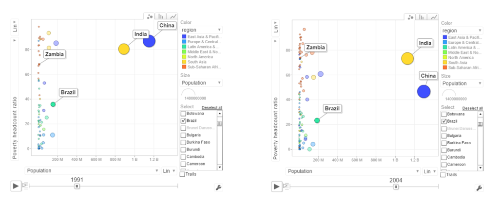
In the early 1990’s China had a higher poverty head count ratio than India. By 2004 China had this all figured out and the poverty head count ratio drops significantly. This can also be seen in the chart below.

pop_pov3

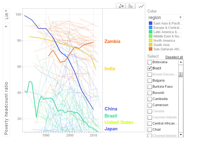
In the chart above China shows a drastic reduction in poverty headcount ratio vs India. Strangely Zambia shows an increase in the poverty head count ratio.

6.Get the data for the 2nd set of indicators

  1. Total population  – SP.POP.TOTL
  2. GDP in US$ – NY.GDP.MKTP.CD
  3. Access to electricity (% population) – EG.ELC.ACCS.ZS
  4. Electricity consumption KWh per capita -EG.USE.ELEC.KH.PC
  5. CO2 emissions -EN.ATM.CO2E.KT
  6. Sanitation Access – SH.STA.ACSN
# World population
population = WDI(indicator='SP.POP.TOTL', country="all",start=1960, end=2016)
# GDP in US $
gdp= WDI(indicator='NY.GDP.MKTP.CD', country="all",start=1960, end=2016)
# Access to electricity (% population)
elecAccess= WDI(indicator='EG.ELC.ACCS.ZS', country="all",start=1960, end=2016)
# Electric power consumption Kwh per capita
elecConsumption= WDI(indicator='EG.USE.ELEC.KH.PC', country="all",start=1960, end=2016)
#CO2 emissions
co2Emissions= WDI(indicator='EN.ATM.CO2E.KT', country="all",start=1960, end=2016)
# Access to sanitation (% population)
sanitationAccess= WDI(indicator='SH.STA.ACSN', country="all",start=1960, end=2016)

7.Rename the columns

names(population)[3]="Total population"
names(gdp)[3]="GDP US($)"
names(elecAccess)[3]="Access to Electricity (% popn)"
names(elecConsumption)[3]="Electric power consumption (KWH per capita)"
names(co2Emissions)[3]="CO2 emisions"
names(sanitationAccess)[3]="Access to sanitation(% popn)"

8.Join the individual data frames

Join the individual data frames to one large wide data frame with all the indicators for the countries


j1 <- join(population, gdp)
j2 <- join(j1,elecAccess)
j3 <- join(j2,elecConsumption)
j4 <- join(j3,co2Emissions)
wbData1 <- join(j3,sanitationAccess)


9.Use WDI_data

Use WDI_data to get the list of indicators and the countries. Join the countries and region

#This returns  list of 2 matrixes
wdi_data =WDI_data
# The 1st matrix is the list is the set of all World Bank Indicators
indicators=wdi_data[[1]]
# The 2nd  matrix gives the set of countries and regions
countries=wdi_data[[2]]
df = as.data.frame(countries)
aa <- df$region != "Aggregates"
# Remove the aggregates
countries_df <- df[aa,]
# Subset from the development data only those corresponding to the countries
ee = subset(wbData1, country %in% countries_df$country)
ff = join(ee,countries_df)
## Joining by: iso2c, country

10.Create and display the motion chart

gg1<- gvisMotionChart(ff,
                                idvar = "country",
                                timevar = "year",
                                xvar = "GDP",
                                yvar = "Access to Electricity",
                                sizevar ="Population",
                                colorvar = "region")
plot(gg1)
cat(gg1$html$chart, file="chart2.html")

This is World Bank Motion Chart2  which has a different set of parameters like Access to Energy, CO2 emissions etc

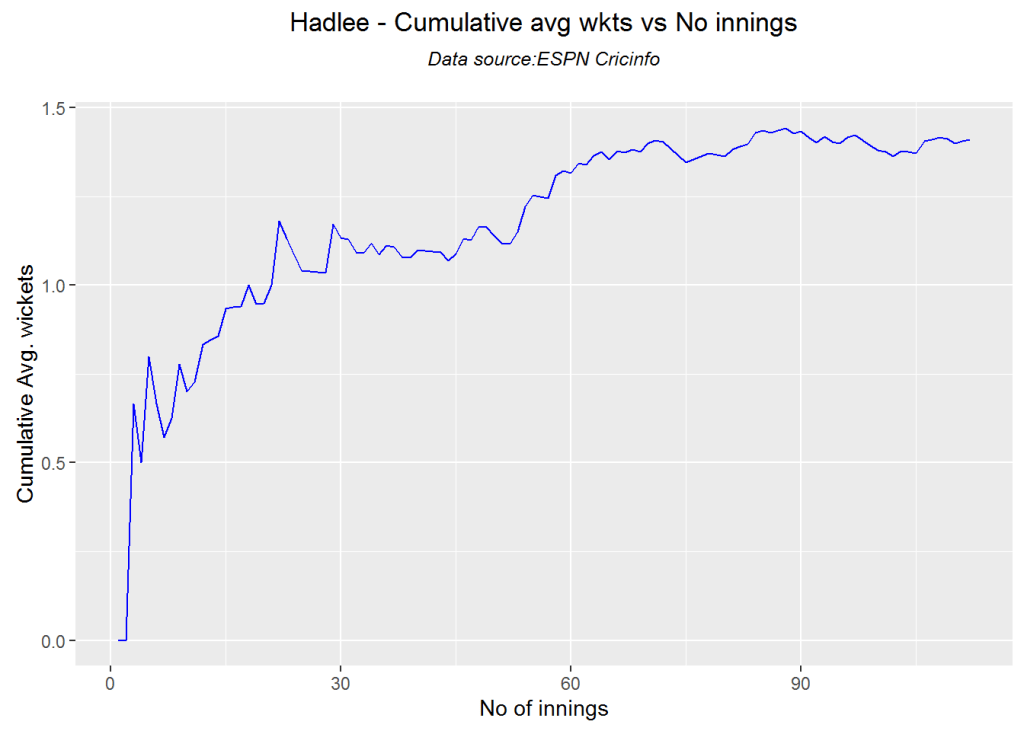
The set of charts below are screenshots of the motion chart World Bank Motion Chart 2

a. Access to Electricity vs Population
pic6
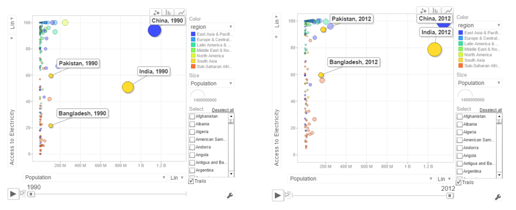
The above chart shows that in China 100% population have access to electricity. India has made decent progress from 50% in 1990 to 79% in 2012. However Pakistan seems to have been much better in providing access to electricity. Pakistan moved from 59% to close 98% access to electricity

b. Power consumption vs population

powercon

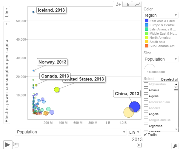
The above chart shows the Power consumption vs Population. China and India have proportionally much lower consumption that Norway, US, Canada

c. CO2 emissions vs Population

pic7

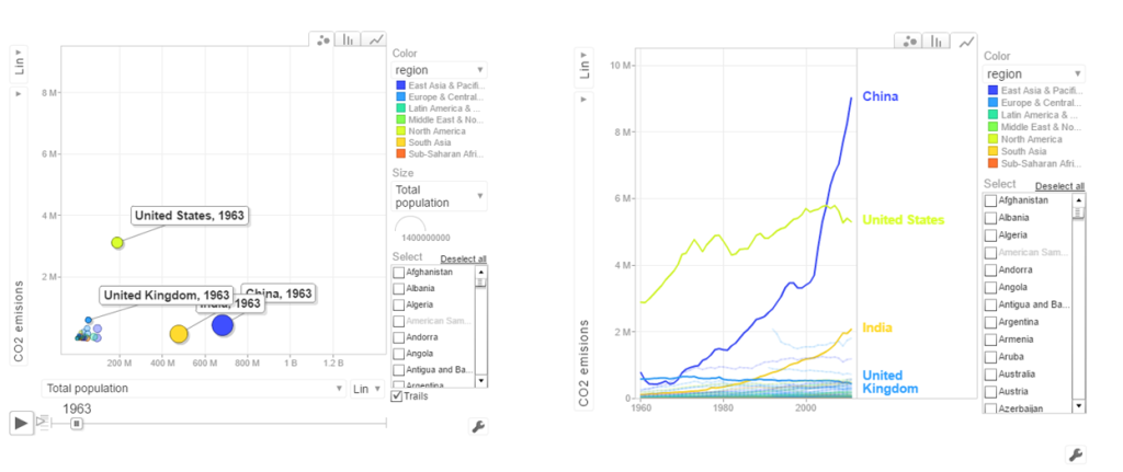
In 1963 the CO2 emissions were fairly low and about comparable for all countries. US, India have shown a steady increase while China shows a steep increase. Interestingly UK shows a drop in CO2 emissions

d.  Access to sanitation
san

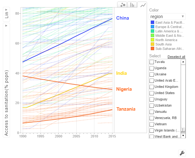
India shows an improvement but it has a long way to go with only 40% of population with access to sanitation. China has made much better strides with 80% having access to sanitation in 2015. Strangely Nigeria shows a drop in sanitation by almost about 20% of population.

The code is available at Github at worldBankAnalysys

Conclusion: So there you have it. I have shown some screenshots of some sample parameters of the World indicators. Please try to play around with World Bank Motion Chart1 & World Bank Motion Chart 2  with your own set of parameters and countries.  You can also create your own motion chart from the 100s of WDI indicators avaialable at  World Bank Data indicator.

Finally, I  would really like to thank Prof Hans Rosling, googleVis and  WDI (Vincent  Arel-Bundock) for making this visualization possible!

Also see
1.  Introducing QCSimulator: A 5-qubit quantum computing simulator in R
2. Dabbling with Wiener filter using OpenCV
3. Designing a Social Web Portal
4. Design Principles of Scalable, Distributed Systems
5. Re-introducing cricketr! : An R package to analyze performances of cricketers
6. Natural language processing: What would Shakespeare say?

To see all posts Index of posts

cricketr sizes up legendary All-rounders of yesteryear

Introduction

This is a post I have been wanting to write for several months, but had to put it off for one reason or another. In this post I use my R package cricketr to analyze the performance of All-rounder greats namely Kapil Dev, Ian Botham, Imran Khan and Richard Hadlee. All these players had talent that was natural and raw. They were good strikers of the ball and extremely lethal with their bowling. The ODI data for these players have been taken from ESPN Cricinfo.

Please be mindful of the ESPN Cricinfo Terms of Use

If you are passionate about cricket, and love analyzing cricket performances, then check out my racy book on cricket ‘Cricket analytics with cricketr and cricpy – Analytics harmony with R & Python’! This book discusses and shows how to use my R package ‘cricketr’ and my Python package ‘cricpy’ to analyze batsmen and bowlers in all formats of the game (Test, ODI and T20). The paperback is available on Amazon at $21.99 and  the kindle version at $9.99/Rs 449/-. A must read for any cricket lover! Check it out!!

You can download the latest PDF version of the book  at  ‘Cricket analytics with cricketr and cricpy: Analytics harmony with R and Python-6th edition

Untitled

You can also read this post at Rpubs as cricketr-AR. Dowload this report as a PDF file from cricketr-AR

Important note 1: The latest release of ‘cricketr’ now includes the ability to analyze performances of teams now!!  See Cricketr adds team analytics to its repertoire!!!

Important note 2 : Cricketr can now do a more fine-grained analysis of players, see Cricketr learns new tricks : Performs fine-grained analysis of players

Important note 3: Do check out the python avatar of cricketr, ‘cricpy’ in my post ‘Introducing cricpy:A python package to analyze performances of cricketers

Note: If you would like to do a similar analysis for a different set of batsman and bowlers, you can clone/download my skeleton cricketr template from Github (which is the R Markdown file I have used for the analysis below). You will only need to make appropriate changes for the players you are interested in. Just a familiarity with R and R Markdown only is needed.

Important note: Do check out my other posts using cricketr at cricketr-posts

All Rounders

  1. Kapil Dev (Ind)
  2. Ian Botham (Eng)
  3. Imran Khan (Pak)
  4. Richard Hadlee (NZ)

I have sprinkled the plots with a few of my comments. Feel free to draw your conclusions! The analysis is included below

if (!require("cricketr")){ 
    install.packages("cricketr",) 
} 

library(cricketr)

The data for any particular ODI player can be obtained with the getPlayerDataOD() function. To do you will need to go to ESPN CricInfo Playerand type in the name of the player for e.g Kapil Dev, etc. This will bring up a page which have the profile number for the player e.g. for Kapil Dev this would be http://www.espncricinfo.com/india/content/player/30028.html. Hence, Kapils’s profile is 30028. This can be used to get the data for Kapil Dev’s data as shown below. I have already executed the below 4 commands and I will use the files to run further commands

#kapil1 
#botham11 
#imran1 
#hadlee1 

Analyses of batting performances of the All Rounders

The following plots gives the analysis of the 4 ODI batsmen

  1. Kapil Dev (Ind) – Innings – 225, Runs = 3783, Average=23.79, Strike Rate= 95.07
  2. Ian Botham (Eng) – Innings – 116, Runs= 2113, Average=23.21, Strike Rate= 79.10
  3. Imran Khan (Pak) – Innings – 175, Runs= 3709, Average=33.41, Strike Rate= 72.65
  4. Richard Hadlee (NZ) – Innings – 115, Runs= 1751, Average=21.61, Strike Rate= 75.50

Plot of 4s, 6s and the scoring rate in ODIs

The 3 charts below give the number of

  1. 4s vs Runs scored
  2. 6s vs Runs scored
  3. Balls faced vs Runs scored

A regression line is fitted in each of these plots for each of the ODI batsmen

A. Kapil Dev
It can be seen that Kapil scores four 4’s when he scores 50. Also after facing 50 deliveries he scores around 43

par(mfrow=c(1,3))
par(mar=c(4,4,2,2))
batsman4s("./kapil1.csv","Kapil")
batsman6s("./kapil1.csv","Kapil")
batsmanScoringRateODTT("./kapil1.csv","Kapil")

kapil-4s6ssr-1

dev.off()
## null device 
##           1

B. Ian Botham
Botham scores around 39 runs after 50 deliveries

par(mfrow=c(1,3))
par(mar=c(4,4,2,2))
batsman4s("./botham1.csv","Botham")
batsman6s("./botham1.csv","Botham")
batsmanScoringRateODTT("./botham1.csv","Botham")

botham-4s6sr-1

dev.off()
## null device 
##           1

C. Imran Khan
Imran scores around 36 runs for 50 deliveries

par(mfrow=c(1,3))
par(mar=c(4,4,2,2))
batsman4s("./imran1.csv","Imran")
batsman6s("./imran1.csv","Imran")
batsmanScoringRateODTT("./imran1.csv","Imran")

imran-4s6ssr-1

dev.off()
## null device 
##           1

D. Richard Hadlee
Hadlee also scores around 30 runs facing 50 deliveries

par(mfrow=c(1,3))
par(mar=c(4,4,2,2))
batsman4s("./hadlee1.csv","Hadlee")
batsman6s("./hadlee1.csv","Hadlee")
batsmanScoringRateODTT("./hadlee1.csv","Hadlee")

hadlee-4s6sout-1

dev.off()
## null device 
##           1

Cumulative Average runs of batsman in career

Kapils cumulative avrerage runs drops towards the last 15 innings wheres Botham had a good run towards the end of his career. Imran performance as a batsman really peaks towards the end with a cumulative average of almost 25 runs. Hadlee has a stead performance

par(mfrow=c(2,2))
par(mar=c(4,4,2,2))
batsmanCumulativeAverageRuns("./kapil1.csv","Kapil")

kbih-car-1

batsmanCumulativeAverageRuns("./botham1.csv","Botham")

kbih-car-2

batsmanCumulativeAverageRuns("./imran1.csv","Imran")

kbih-car-3

batsmanCumulativeAverageRuns("./hadlee1.csv","Hadlee")

kbih-car-4

dev.off()
## null device 
##           1

Cumulative Average strike rate of batsman in career

Kapil’s strike rate is superlative touching the 90’s steadily. Botham’s strike drops dramatically towards the latter part of his career. Imran average at a steady 75 and Hadlee averages around 85.

par(mfrow=c(2,2))
par(mar=c(4,4,2,2))
batsmanCumulativeStrikeRate("./kapil1.csv","Kapil")

kbih-casr-1

batsmanCumulativeStrikeRate("./botham1.csv","Botham")

kbih-casr-2

batsmanCumulativeStrikeRate("./imran1.csv","Imran")

kbih-casr-3

batsmanCumulativeStrikeRate("./hadlee1.csv","Hadlee")

kbih-casr-4

dev.off()
## null device 
##           1

Relative Mean Strike Rate

Kapil tops the strike rate among all the all-rounders. This is really a revelation to me. This can also be seen in the original data in Kapil’s strike rate is at a whopping 95.07 in comparison to Botham, Inran and Hadlee who are at 79.1,72.65 and 75.50 respectively

par(mar=c(4,4,2,2))
frames <- list("./kapil1.csv","./botham1.csv","imran1.csv","hadlee1.csv")
names <- list("Kapil","Botham","Imran","Hadlee")
relativeBatsmanSRODTT(frames,names)

plot-1-1

Relative Runs Frequency Percentage

This plot shows that Imran has a much better average runs scored over the other all rounders followed by Kapil

frames <- list("./kapil1.csv","./botham1.csv","imran1.csv","hadlee1.csv")
names <- list("Kapil","Botham","Imran","Hadlee")
relativeRunsFreqPerfODTT(frames,names)

plot-2-1

Relative cumulative average runs in career

It can be seen clearly that Imran Khan leads the pack in cumulative average runs followed by Kapil Dev and then Botham

frames <- list("./kapil1.csv","./botham1.csv","imran1.csv","hadlee1.csv")
names <- list("Kapil","Botham","Imran","Hadlee")
relativeBatsmanCumulativeAvgRuns(frames,names)

kbih-relcar-1

Relative cumulative average strike rate in career

In the cumulative strike rate Hadlee and Kapil run a close race.

frames <- list("./kapil1.csv","./botham1.csv","imran1.csv","hadlee1.csv")
names <- list("Kapil","Botham","Imran","Hadlee")
relativeBatsmanCumulativeStrikeRate(frames,names)

kbih-relcsr-1

Percent 4’s,6’s in total runs scored

The plot below shows the contrib

frames <- list("./kapil1.csv","./botham1.csv","imran1.csv","hadlee1.csv")
names <- list("Kapil","Botham","Imran","Hadlee")
runs4s6s <-batsman4s6s(frames,names)

plot-46s-1

print(runs4s6s)
##                Kapil Botham Imran Hadlee
## Runs(1s,2s,3s) 72.08  66.53 77.53  73.27
## 4s             21.98  25.78 17.61  21.08
## 6s              5.94   7.68  4.86   5.65

Runs forecast

The forecast for the batsman is shown below.

par(mfrow=c(2,2))
par(mar=c(4,4,2,2))
batsmanPerfForecast("./kapil1.csv","Kapil")
batsmanPerfForecast("./botham1.csv","Botham")
batsmanPerfForecast("./imran1.csv","Imran")
batsmanPerfForecast("./hadlee1.csv","Hadlee")

plot-fcst-1

dev.off()
## null device 
##           1

3D plot of Runs vs Balls Faced and Minutes at Crease

The plot is a scatter plot of Runs vs Balls faced and Minutes at Crease. A prediction plane is fitted

par(mfrow=c(1,2))
par(mar=c(4,4,2,2))
battingPerf3d("./kapil1.csv","Kapil")
battingPerf3d("./botham1.csv","Botham")

plot-3-1

dev.off()
## null device 
##           1
par(mfrow=c(1,2))
par(mar=c(4,4,2,2))
battingPerf3d("./imran1.csv","Imran")
battingPerf3d("./hadlee1.csv","Hadlee")

plot-4-1

dev.off()
## null device 
##           1

Predicting Runs given Balls Faced and Minutes at Crease

A multi-variate regression plane is fitted between Runs and Balls faced +Minutes at crease.

BF <- seq( 10, 200,length=10)
Mins <- seq(30,220,length=10)
newDF <- data.frame(BF,Mins)

kapil <- batsmanRunsPredict("./kapil1.csv","Kapil",newdataframe=newDF)
botham <- batsmanRunsPredict("./botham1.csv","Botham",newdataframe=newDF)
imran <- batsmanRunsPredict("./imran1.csv","Imran",newdataframe=newDF)
hadlee <- batsmanRunsPredict("./hadlee1.csv","Hadlee",newdataframe=newDF)

The fitted model is then used to predict the runs that the batsmen will score for a hypotheticial Balls faced and Minutes at crease. It can be seen that Kapil is the best bet for a balls faced and minutes at crease followed by Botham.

batsmen <-cbind(round(kapil$Runs),round(botham$Runs),round(imran$Runs),round(hadlee$Runs))
colnames(batsmen) <- c("Kapil","Botham","Imran","Hadlee")
newDF <- data.frame(round(newDF$BF),round(newDF$Mins))
colnames(newDF) <- c("BallsFaced","MinsAtCrease")
predictedRuns <- cbind(newDF,batsmen)
predictedRuns
##    BallsFaced MinsAtCrease Kapil Botham Imran Hadlee
## 1          10           30    16      6    10     15
## 2          31           51    33     22    22     28
## 3          52           72    49     38    33     42
## 4          73           93    65     54    45     56
## 5          94          114    81     70    56     70
## 6         116          136    97     86    67     84
## 7         137          157   113    102    79     97
## 8         158          178   130    117    90    111
## 9         179          199   146    133   102    125
## 10        200          220   162    149   113    139

Highest runs likelihood

The plots below the runs likelihood of batsman. This uses K-Means . A. Kapil Dev

batsmanRunsLikelihood("./kapil1.csv","Kapil")

kapil11-1

## Summary of  Kapil 's runs scoring likelihood
## **************************************************
## 
## There is a 34.57 % likelihood that Kapil  will make  22 Runs in  24 balls over 34  Minutes 
## There is a 17.28 % likelihood that Kapil  will make  46 Runs in  46 balls over  65  Minutes 
## There is a 48.15 % likelihood that Kapil  will make  5 Runs in  7 balls over 9  Minutes

B. Ian Botham

batsmanRunsLikelihood("./botham1.csv","Botham")

devilliers-1

## Summary of  Botham 's runs scoring likelihood
## **************************************************
## 
## There is a 47.95 % likelihood that Botham  will make  9 Runs in  12 balls over 15  Minutes 
## There is a 39.73 % likelihood that Botham  will make  23 Runs in  32 balls over  44  Minutes 
## There is a 12.33 % likelihood that Botham  will make  59 Runs in  74 balls over 101  Minutes

C. Imran Khan

batsmanRunsLikelihood("./imran1.csv","Imran")

gaylecache-true-1

## Summary of  Imran 's runs scoring likelihood
## **************************************************
## 
## There is a 23.33 % likelihood that Imran  will make  36 Runs in  54 balls over 74  Minutes 
## There is a 60 % likelihood that Imran  will make  14 Runs in  18 balls over  23  Minutes 
## There is a 16.67 % likelihood that Imran  will make  53 Runs in  90 balls over 115  Minutes

D. Richard Hadlee

batsmanRunsLikelihood("./hadlee1.csv","Hadlee")

maxwell-1

## Summary of  Hadlee 's runs scoring likelihood
## **************************************************
## 
## There is a 6.1 % likelihood that Hadlee  will make  64 Runs in  79 balls over 90  Minutes 
## There is a 42.68 % likelihood that Hadlee  will make  25 Runs in  33 balls over  44  Minutes 
## There is a 51.22 % likelihood that Hadlee  will make  9 Runs in  11 balls over 15  Minutes

Average runs at ground and against opposition

A. Kapil Dev

par(mfrow=c(1,2))
par(mar=c(4,4,2,2))
batsmanAvgRunsGround("./kapil1.csv","Kapil")
batsmanAvgRunsOpposition("./kapil1.csv","Kapil")

avgrg-1-1

dev.off()
## null device 
##           1

B. Ian Botham

par(mfrow=c(1,2))
par(mar=c(4,4,2,2))
batsmanAvgRunsGround("./botham1.csv","Botham")
batsmanAvgRunsOpposition("./botham1.csv","Botham")

avgrg-2-1

dev.off()
## null device 
##           1

C. Imran Khan

par(mfrow=c(1,2))
par(mar=c(4,4,2,2))
batsmanAvgRunsGround("./imran1.csv","Imran")
batsmanAvgRunsOpposition("./imran1.csv","Imran")

avgrg-3-1

dev.off()
## null device 
##           1

D. Richard Hadlee

par(mfrow=c(1,2))
par(mar=c(4,4,2,2))
batsmanAvgRunsGround("./hadlee1.csv","Hadlee")
batsmanAvgRunsOpposition("./hadlee1.csv","Hadlee")

avgrg-4-1

dev.off()
## null device 
##           1

Moving Average of runs over career

The moving average for the 4 batsmen indicate the following

Kapil’s performance drops significantly while there is a slump in Botham’s performance. On the other hand Imran and Hadlee’s performance were on the upswing.

par(mfrow=c(2,2))
par(mar=c(4,4,2,2))
batsmanMovingAverage("./kapil1.csv","Kapil")
batsmanMovingAverage("./botham1.csv","Botham")
batsmanMovingAverage("./imran1.csv","Imran")
batsmanMovingAverage("./hadlee1.csv","Hadlee")

sdgm-ma-1

dev.off()
## null device 
##           1

Check batsmen in-form, out-of-form

[1] “**************************** Form status of Kapil ****************************\n\n
Population size: 72
Mean of population: 19.38 \n
Sample size: 9 Mean of sample: 6.78 SD of sample: 6.14 \n\n
Null hypothesis H0 : Kapil ‘s sample average is within 95% confidence interval of population average\n
Alternative hypothesis Ha : Kapil ‘s sample average is below the 95% confidence interval of population average\n\n
Kapil ‘s Form Status: Out-of-Form because the p value: 8.4e-05 is less than alpha= 0.05

“**************************** Form status of Botham ****************************\n\n
Population size: 65
Mean of population: 21.29 \n
Sample size: 8 Mean of sample: 15.38 SD of sample: 13.19 \n\n
Null hypothesis H0 : Botham ‘s sample average is within 95% confidence interval of population average\n
Alternative hypothesis Ha : Botham ‘s sample average is below the 95% confidence interval of population average\n\n
Botham ‘s Form Status: In-Form because the p value: 0.120342 is greater than alpha= 0.05 \n

“**************************** Form status of Imran ****************************\n\n
Population size: 54
Mean of population: 24.94 \n
Sample size: 6 Mean of sample: 30.83 SD of sample: 25.4 \n\n
Null hypothesis H0 : Imran ‘s sample average is within 95% confidence interval of population average\n
Alternative hypothesis Ha : Imran ‘s sample average is below the 95% confidence interval of population average\n\n
Imran ‘s Form Status: In-Form because the p value: 0.704683 is greater than alpha= 0.05 \n

“**************************** Form status of Hadlee ****************************\n\n
Population size: 73
Mean of population: 18 \n
Sample size: 9 Mean of sample: 27 SD of sample: 24.27 \n\n
Null hypothesis H0 : Hadlee ‘s sample average is within 95% confidence interval of population average\n
Alternative hypothesis Ha : Hadlee ‘s sample average is below the 95% confidence interval of population average\n\n
Hadlee ‘s Form Status: In-Form because the p value: 0.85262 is greater than alpha= 0.05 \n *******************************************************************************************\n\n”

Analyses of bowling performances of the All Rounders

The following plots gives the analysis of the 4 ODI batsmen

  1. Kapil Dev (Ind) – Innings – 225, Wickets = 253, Average=27.45, Economy Rate= 3.71
  2. Ian Botham (Eng) – Innings – 116, Wickets = 145, Average=28.54, Economy Rate= 3.96
  3. Imran Khan (Pak) – Innings – 175, Wickets = 182, Average=26.61, Economy Rate= 3.89
  4. Richard Hadlee (NZ) – Innings – 115, Wickets = 158, Average=21.56, Economy Rate= 3.30

Botham has the highest number of innings and wickets followed closely by Mitchell. Imran and Hadlee have relatively fewer innings.

To get the bowler’s data use

#kapil2 
#botham2 
#imran2 
#hadlee2 

“`

Wicket Frequency percentage

This plot gives the percentage of wickets for each wickets (1,2,3…etc).

par(mfrow=c(1,4))
par(mar=c(4,4,2,2))
bowlerWktsFreqPercent("./kapil2.csv","Kapil")
bowlerWktsFreqPercent("./botham2.csv","Botham")
bowlerWktsFreqPercent("./imran2.csv","Imran")
bowlerWktsFreqPercent("./hadlee2.csv","Hadlee")

relbowlfp-1

dev.off()
## null device 
##           1

Wickets Runs plot

The plot below gives a boxplot of the runs ranges for each of the wickets taken by the bowlers.

par(mfrow=c(1,4))
par(mar=c(4,4,2,2))

bowlerWktsRunsPlot("./kapil2.csv","Kapil")
bowlerWktsRunsPlot("./botham2.csv","Botham")
bowlerWktsRunsPlot("./imran2.csv","Imran")
bowlerWktsRunsPlot("./hadlee2.csv","Hadlee")

wktsrun-1

dev.off()
## null device 
##           1

Cumulative average wicket plot

Botham has the best cumulative average wicket touching almost 1.6 wickets followed by Hadlee

par(mfrow=c(1,3))
par(mar=c(4,4,2,2))
bowlerCumulativeAvgWickets("./kapil2.csv","Kapil")

kwm-bowlcaw-1

bowlerCumulativeAvgWickets("./botham2.csv","Botham")

kwm-bowlcaw-2

bowlerCumulativeAvgWickets("./imran2.csv","Imran")

kwm-bowlcaw-3

bowlerCumulativeAvgWickets("./hadlee2.csv","Hadlee")

kwm-bowlcaw-4

dev.off()
## null device 
##           1
par(mfrow=c(1,3))
par(mar=c(4,4,2,2))
bowlerCumulativeAvgEconRate("./kapil2.csv","Kapil")

kwm-bowlcer-1

bowlerCumulativeAvgEconRate("./botham2.csv","Botham")

kwm-bowlcer-2

bowlerCumulativeAvgEconRate("./imran2.csv","Imran")

kwm-bowlcer-3

bowlerCumulativeAvgEconRate("./hadlee2.csv","Hadlee")

kwm-bowlcer-4

dev.off()
## null device 
##           1

Average wickets in different grounds and opposition

A. Kapil Dev

par(mfrow=c(1,2))
par(mar=c(4,4,2,2))
bowlerAvgWktsGround("./kapil2.csv","Kapil")
bowlerAvgWktsOpposition("./kapil2.csv","Kapil")

gr-1-1

dev.off()
## null device 
##           1

B. Ian Botham

par(mfrow=c(1,2))
par(mar=c(4,4,2,2))
bowlerAvgWktsGround("./botham2.csv","Botham")
bowlerAvgWktsOpposition("./botham2.csv","Botham")

gr-2-1

dev.off()
## null device 
##           1

C. Imran Khan

par(mfrow=c(1,2))
par(mar=c(4,4,2,2))
bowlerAvgWktsGround("./imran2.csv","Imran")
bowlerAvgWktsOpposition("./imran2.csv","Imran")

gr-3-1

dev.off()
## null device 
##           1

D. Richard Hadlee

par(mfrow=c(1,2))
par(mar=c(4,4,2,2))
bowlerAvgWktsGround("./hadlee2.csv","Hadlee")
bowlerAvgWktsOpposition("./hadlee2.csv","Hadlee")

gr-4-1

dev.off()
## null device 
##           1

Relative bowling performance

It can be seen that Botham is the most effective wicket taker of the lot

frames <- list("./kapil2.csv","./botham2.csv","imran2.csv","hadlee2.csv")
names <- list("Kapil","Botham","Imran","Hadlee")
relativeBowlingPerf(frames,names)

relbowlperf-1

Relative Economy Rate against wickets taken

Hadlee has the best overall economy rate followed by Kapil Dev

frames <- list("./kapil2.csv","./botham2.csv","imran2.csv","hadlee2.csv")
names <- list("Kapil","Botham","Imran","Hadlee")
relativeBowlingERODTT(frames,names)

relbowler-1

Relative cumulative average wickets of bowlers in career

This plot confirms the wicket taking ability of Botham followed by Hadlee

frames <- list("./kapil2.csv","./botham2.csv","imran2.csv","hadlee2.csv")
names <- list("Kapil","Botham","Imran","Hadlee")
relativeBowlerCumulativeAvgWickets(frames,names)

rbcaw-1

Relative cumulative average economy rate of bowlers

frames <- list("./kapil2.csv","./botham2.csv","imran2.csv","hadlee2.csv")
names <- list("Kapil","Botham","Imran","Hadlee")
relativeBowlerCumulativeAvgEconRate(frames,names)

rbcer-1

Moving average of wickets over career

This plot shows that Hadlee has the best economy rate followed by Kapil

par(mfrow=c(2,2))
par(mar=c(4,4,2,2))
bowlerMovingAverage("./kapil2.csv","Kapil")
bowlerMovingAverage("./botham2.csv","Botham")
bowlerMovingAverage("./imran2.csv","Imran")
bowlerMovingAverage("./hadlee2.csv","Hadlee")

jmss-bowlma-1

dev.off()
## null device 
##           1

Wickets forecast

par(mfrow=c(2,2))
par(mar=c(4,4,2,2))
bowlerPerfForecast("./kapil2.csv","Kapil")
bowlerPerfForecast("./botham2.csv","Botham")
bowlerPerfForecast("./imran2.csv","Imran")
bowlerPerfForecast("./hadlee2.csv","Hadlee")

jjmss-pfcst-1

dev.off()
## null device 
##           1

Check bowler in-form, out-of-form

“**************************** Form status of Kapil ****************************\n\n
Population size: 198
Mean of population: 1.2 \n Sample size: 23 Mean of sample: 0.65 SD of sample: 0.83 \n\n
Null hypothesis H0 : Kapil ‘s sample average is within 95% confidence interval \n of population average\n
Alternative hypothesis Ha : Kapil ‘s sample average is below the 95% confidence\n interval of population average\n\n
Kapil ‘s Form Status: Out-of-Form because the p value: 0.002097 is less than alpha= 0.05 \n

“**************************** Form status of Botham ****************************\n\n
Population size: 166
Mean of population: 1.58 \n Sample size: 19 Mean of sample: 1.47 SD of sample: 1.12 \n\n
Null hypothesis H0 : Botham ‘s sample average is within 95% confidence interval \n of population average\n
Alternative hypothesis Ha : Botham ‘s sample average is below the 95% confidence\n interval of population average\n\n
Botham ‘s Form Status: In-Form because the p value: 0.336694 is greater than alpha= 0.05 \n

“**************************** Form status of Imran ****************************\n\n
Population size: 137
Mean of population: 1.23 \n Sample size: 16 Mean of sample: 0.81 SD of sample: 0.91 \n\n
Null hypothesis H0 : Imran ‘s sample average is within 95% confidence interval \n of population average\n
Alternative hypothesis Ha : Imran ‘s sample average is below the 95% confidence\n interval of population average\n\n
Imran ‘s Form Status: Out-of-Form because the p value: 0.041727 is less than alpha= 0.05 \n

“**************************** Form status of Hadlee ****************************\n\n
Population size: 100
Mean of population: 1.38 \n Sample size: 12 Mean of sample: 1.67 SD of sample: 1.37 \n\n
Null hypothesis H0 : Hadlee ‘s sample average is within 95% confidence interval \n of population average\n
Alternative hypothesis Ha : Hadlee ‘s sample average is below the 95% confidence\n interval of population average\n\n
Hadlee ‘s Form Status: In-Form because the p value: 0.761265 is greater than alpha= 0.05 \n *******************************************************************************************\n\n”

Key findings

Here are some key conclusions ODI batsmen

  1. Kapil Dev’s strike rate stands high above the other 3
  2. Imran Khan has the best cumulative average runs followed by Kapil
  3. Botham is the most effective wicket taker followed by Hadlee
  4. Hadlee is the most economical bowler and is followed by Kapil Dev
  5. For a hypothetical Balls Faced and Minutes at creases Kapil will score the most runs followed by Botham
  6. The moving average of indicates that the best is yet to come for Imran and Hadlee. Kapil and Botham were on the decline

Also see my other posts in R

  1. A primer on Qubits, Quantum gates abd Quantum operations
  2. Deblurring with OpenCV:Weiner filter reloaded
  3. Designing a Social Web Portal
  4. A crime map of India in R – Crimes against women
  5. Bend it like Bluemix, MongoDB with autoscaling – Part 2
  6. Mirror, mirror . the best batsman of them all?

For a full list of posts see Index of posts

IBM Data Science Experience:  First steps with yorkr

Fresh, and slightly dizzy, from my foray into Quantum Computing with IBM’s Quantum Experience, I now turn my attention to IBM’s Data Science Experience (DSE).

I am on the verge of completing a really great 3 module ‘Data Science and Engineering with Spark XSeries’ from the University of California, Berkeley and I have been thinking of trying out some form of integrated delivery platform for performing analytics, for quite some time.  Coincidentally,  IBM comes out with its Data Science Experience. a month back. There are a couple of other collaborative platforms available for playing around with Apache Spark or Data Analytics namely Jupyter notebooks, Databricks, Data.world.

I decided to go ahead with IBM’s Data Science Experience as  the GUI is a lot cooler, includes shared data sets and integrates with Object Storage, Cloudant DB etc,  which seemed a lot closer to the cloud, literally!  IBM’s DSE is an interactive, collaborative, cloud-based environment for performing data analysis with Apache Spark. DSE is hosted on IBM’s PaaS environment, Bluemix. It should be possible to access in DSE the plethora of cloud services available on Bluemix. IBM’s DSE uses Jupyter notebooks for creating and analyzing data which can be easily shared and has access to a few hundred publicly available datasets

Disclaimer: This article represents the author’s viewpoint only and doesn’t necessarily represent IBM’s positions, strategies or opinions

In this post, I use IBM’s DSE and my R package yorkr, for analyzing the performance of 1 ODI match (Aus-Ind, 2 Feb 2012)  and the batting performance of Virat Kohli in IPL matches. These are my ‘first’ steps in DSE so, I use plain old “R language” for analysis together with my R package ‘yorkr’. I intend to  do more interesting stuff on Machine learning with SparkR, Sparklyr and PySpark in the weeks and months to come.

You can checkout the Jupyter notebooks created with IBM’s DSE Y at Github  – “Using R package yorkr – A quick overview’ and  on NBviewer at “Using R package yorkr – A quick overview

Working with Jupyter notebooks are fairly straight forward which can handle code in R, Python and Scala. Each cell can either contain code (Python or Scala), Markdown text, NBConvert or Heading. The code is written into the cells and can be executed sequentially. Here is a screen shot of the notebook.

Untitled

The ‘File’ menu can be used for ‘saving and checkpointing’ or ‘reverting’ to a checkpoint. The ‘kernel’ menu can be used to start, interrupt, restart and run all cells etc. Data Sources icon can be used to load data sources to your code. The data is uploaded to Object Storage with appropriate credentials. You will have to  import this data from Object Storage using the credentials. In my notebook with yorkr I directly load the data from Github.  You can use the sharing to share the notebook. The shared notebook has an extension ‘ipynb’. You can use the ‘Sharing’ icon  to share the notebook. The shared notebook has an extension ‘ipynb’. You an import this notebook directly into your environment and can get started with the code available in the notebook.

You can import existing R, Python or Scala notebooks as shown below. My notebook ‘Using R package yorkr – A quick overview’ can be downloaded using the link ‘yorkrWithDSE’ and clicking the green download icon on top right corner.

Untitled2

I have also uploaded the file to Github and you can download from here too ‘yorkrWithDSE’. This notebook can be imported into your DSE as shown below

Untitled1

Jupyter notebooks have been integrated with Github and are rendered directly from Github.  You can view my Jupyter notebook here  – “Using R package yorkr – A quick overview’. You can also view it on NBviewer at “Using R package yorkr – A quick overview

So there it is. You can download my notebook, import it into IBM’s Data Science Experience and then use data from ‘yorkrData” as shown. As already mentioned yorkrData contains converted data for ODIs, T20 and IPL. For details on how to use my R package yorkr  please my posts on yorkr at “Index of posts

Hope you have fun playing wit IBM’s Data Science Experience and my package yorkr.

I will be exploring IBM’s DSE in weeks and months to come in the areas of Machine Learning with SparkR,SparklyR or pySpark.

Watch this space!!!

Disclaimer: This article represents the author’s viewpoint only and doesn’t necessarily represent IBM’s positions, strategies or opinions

Also see

1. Introducing QCSimulator: A 5-qubit quantum computing simulator in R
2. Natural Processing Language : What would Shakespeare say?
3. Introducing cricket package yorkr:Part 1- Beaten by sheer pace!
4. A closer look at “Robot horse on a Trot! in Android”
5.  Re-introducing cricketr! : An R package to analyze performances of cricketers
6.   What’s up Watson? Using IBM Watson’s QAAPI with Bluemix, NodeExpress – Part 1
7.  Deblurring with OpenCV: Wiener filter reloaded

To see all my posts check
Index of posts