In this post I introduce my new Shiny app,“GooglyPlus”, which is a more evolved version of my earlier Shiny app “Googly”. My R package ‘yorkr’, on which both these Shiny apps are based, has the ability to output either a dataframe or plot, depending on a parameter plot=TRUE or FALSE. My initial version of the app only included plots, and did not exercise the yorkr package fully. Moreover, I am certain, there may be a set of cricket aficionados who would prefer, numbers to charts. Hence I have created this enhanced version of the Googly app and appropriately renamed it as GooglyPlus. GooglyPlus is based on the yorkr package which uses data from Cricsheet. The app is based on IPL data from all IPL matches from 2008 up to 2016. Feel free to clone/fork or download the code from Github at GooglyPlus.
If you are passionate about cricket, and love analyzing cricket performances, then check out my 2 racy books on cricket! In my books, I perform detailed yet compact analysis of performances of both batsmen, bowlers besides evaluating team & match performances in Tests , ODIs, T20s & IPL. You can buy my books on cricket from Amazon at $12.99 for the paperback and $4.99/$6.99 respectively for the kindle versions. The books can be accessed at Cricket analytics with cricketr and Beaten by sheer pace-Cricket analytics with yorkr A must read for any cricket lover! Check it out!!
Click GooglyPlus to access the Shiny app!
The changes for GooglyPlus over the earlier Googly app is only in the following 3 tab panels
- IPL match
- Head to head
- Overall Performance
The analysis of IPL batsman and IPL bowler tabs are unchanged. These charts are as they were before.
The changes are only in tabs i) IPL match ii) Head to head and iii) Overall Performance. New functionality has been added and existing functions now have the dual option of either displaying a plot or a table.
The changes are
A) IPL Match
The following additions/enhancements have been done
-Match Batting Scorecard – Table
-Batting Partnerships – Plot, Table (New)
-Batsmen vs Bowlers – Plot, Table(New)
-Match Bowling Scorecard – Table (New)
-Bowling Wicket Kind – Plot, Table (New)
-Bowling Wicket Runs – Plot, Table (New)
-Bowling Wicket Match – Plot, Table (New)
-Bowler vs Batsmen – Plot, Table (New)
-Match Worm Graph – Plot
B) Head to head
The following functions have been added/enhanced
-Team Batsmen Batting Partnerships All Matches – Plot, Table {Summary (New) and Detailed (New)}
-Team Batting Scorecard All Matches – Table (New)
-Team Batsmen vs Bowlers all Matches – Plot, Table (New)
-Team Wickets Opposition All Matches – Plot, Table (New)
-Team Bowling Scorecard All Matches – Table (New)
-Team Bowler vs Batsmen All Matches – Plot, Table (New)
-Team Bowlers Wicket Kind All Matches – Plot, Table (New)
-Team Bowler Wicket Runs All Matches – Plot, Table (New)
-Win Loss All Matches – Plot
C) Overall Performance
The following additions/enhancements have been done in this tab
-Team Batsmen Partnerships Overall – Plot, Table {Summary (New) and Detailed (New)}
-Team Batting Scorecard Overall –Table (New)
-Team Batsmen vs Bowlers Overall – Plot, Table (New)
-Team Bowler vs Batsmen Overall – Plot, Table (New)
-Team Bowling Scorecard Overall – Table (New)
-Team Bowler Wicket Kind Overall – Plot, Table (New)
Included below are some random charts and tables. Feel free to explore the Shiny app further
1) IPL Match
a) Match Batting Scorecard (Table only)
This is the batting score card for the Chennai Super Kings & Deccan Chargers 2011-05-11

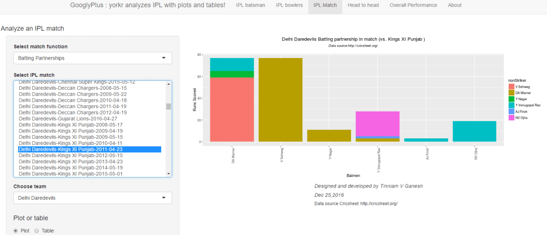
b) Match batting partnerships (Plot)
Delhi Daredevils vs Kings XI Punjab – 2011-04-23
c) Match batting partnerships (Table)
The same batting partnership Delhi Daredevils vs Kings XI Punjab – 2011-04-23 as a table

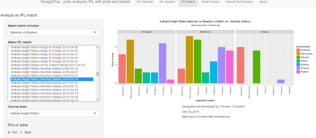
d) Batsmen vs Bowlers (Plot)
Kolkata Knight Riders vs Mumbai Indians 2010-04-19
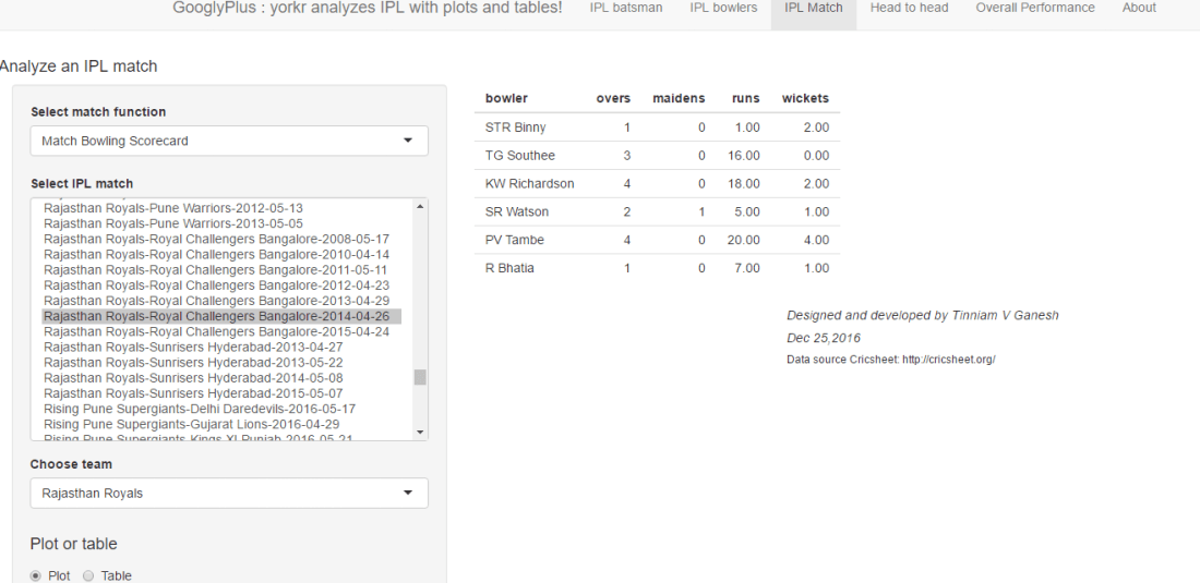
e) Match Bowling Scorecard (Table only)
B) Head to head
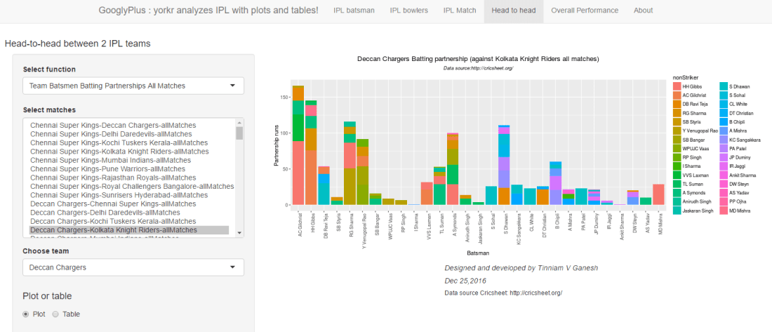
a) Team Batsmen Partnership (Plot)
Deccan Chargers vs Kolkata Knight Riders all matches
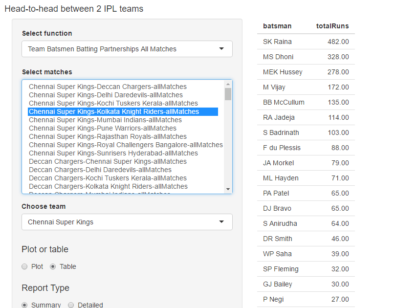
b) Team Batsmen Partnership (Summary – Table)
In the following tables it can be seen that MS Dhoni has performed better that SK Raina CSK against DD matches, whereas SK Raina performs better than Dhoni in CSK vs KKR matches
i) Chennai Super Kings vs Delhi Daredevils (Summary – Table)

ii) Chennai Super Kings vs Kolkata Knight Riders (Summary – Table)
iii) Rising Pune Supergiants vs Gujarat Lions (Detailed – Table)
This table provides the detailed partnership for RPS vs GL all matches

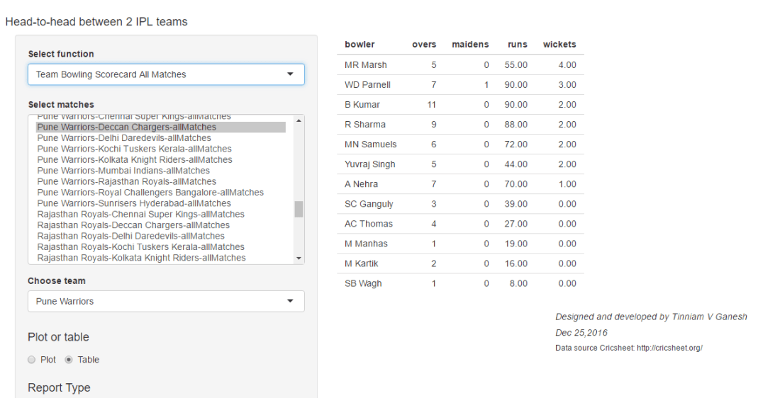
c) Team Bowling Scorecard (Table only)
This table gives the bowling scorecard of Pune Warriors vs Deccan Chargers in all matches
C) Overall performances
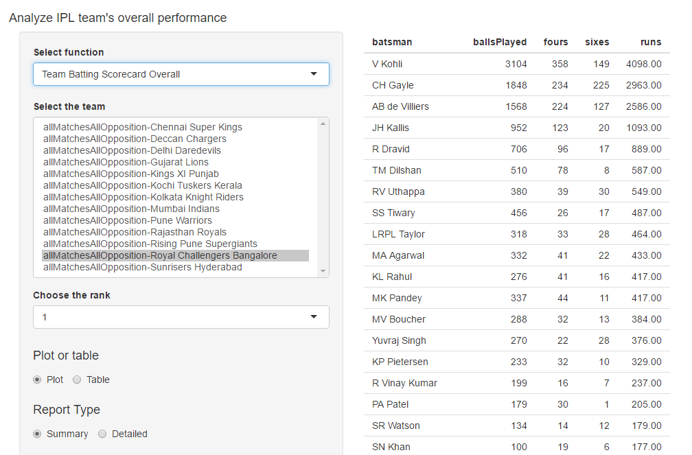
a) Batting Scorecard All Matches (Table only)
This is the batting scorecard of Royal Challengers Bangalore. The top 3 batsmen are V Kohli, C Gayle and AB Devilliers in that order
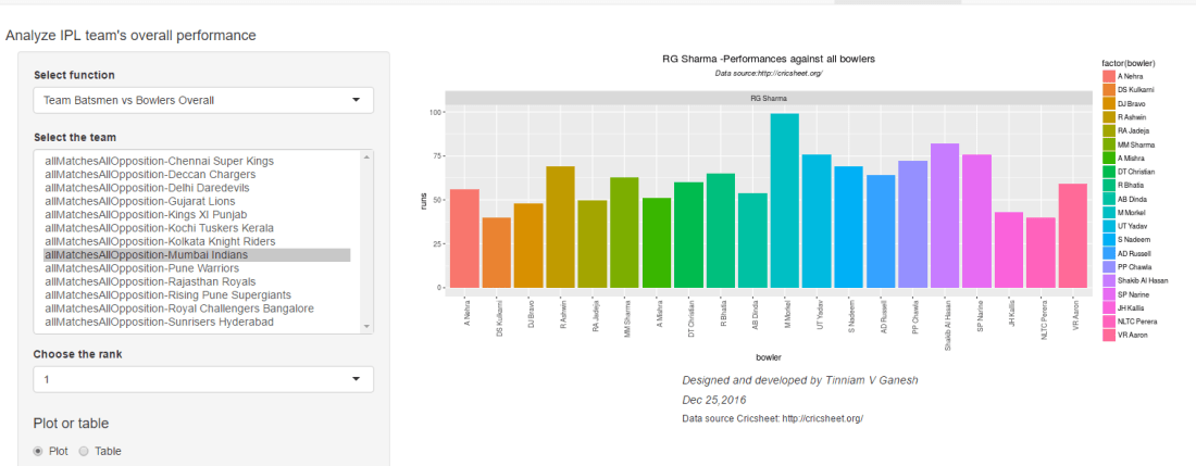
b) Batsman vs Bowlers all Matches (Plot)
This gives the performance of Mumbai Indian’s batsman of Rank=1, which is Rohit Sharma, against bowlers of all other teams
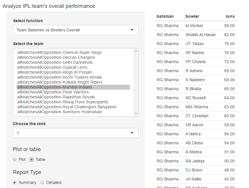
c) Batsman vs Bowlers all Matches (Table)
The above plot as a table. It can be seen that Rohit Sharma has scored maximum runs against M Morkel, then Shakib Al Hasan and then UT Yadav.
d) Bowling scorecard (Table only)
The table below gives the bowling scorecard of CSK. R Ashwin leads with a tally of 98 wickets followed by DJ Bravo who has 88 wickets and then JA Morkel who has 83 wickets in all matches against all teams

This is just a random selection of functions. Do play around with the app and checkout how the different IPL batsmen, bowlers and teams stack against each other. Do read my earlier post Googly: An interactive app for analyzing IPL players, matches and teams using R package yorkr for more details about the app and other functions available.
Click GooglyPlus to access the Shiny app!
You can clone/fork/download the code from Github at GooglyPlus
Hope you have fun playing around with the Shiny app!
Note: In the tabs, for some of the functions, not all controls are required. It is possible to enable the controls selectively but this has not been done in this current version. I may make the changes some time in the future.
Take a look at my other Shiny apps
a.Revisiting crimes against women in India
b. Natural language processing: What would Shakespeare say?
Check out some of my other posts
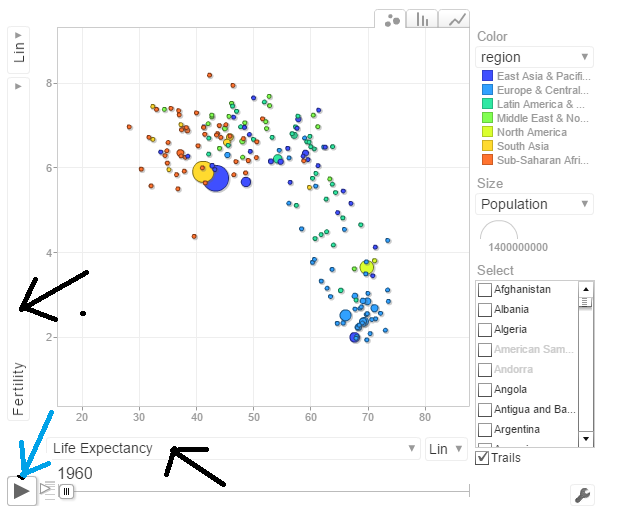
1. Analyzing World Bank data with WDI, googleVis Motion Charts
2. Video presentation on Machine Learning, Data Science, NLP and Big Data – Part 1
3. Singularity
4. Design principles of scalable, distributed systems
5. Simulating an Edge shape in Android
6. Dabbling with Wiener filter in OpenCV
To see all posts click Index of Posts


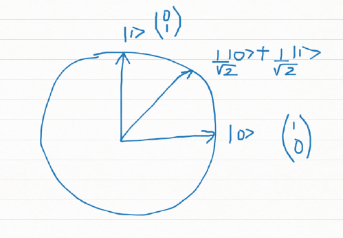
 and |1> =
 |0> =
|0> = 


 – (A)
– (A)


 and | β|2 = =

 representing the state of the electron
 and
and  then |0> =
 and
and  then |1> =
 with |0>
 is the projection of on one of the standard basis |0> or |1>
 and
and
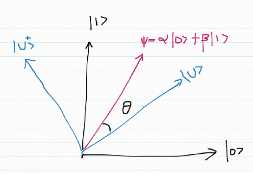
 with |u> then we can write


 which makes 60 degrees with the |0> basis
 which is the diagonal |+> basis

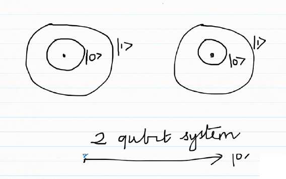

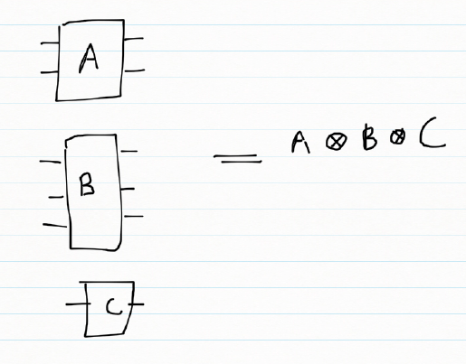
 is the tensor product
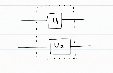


 *
* 


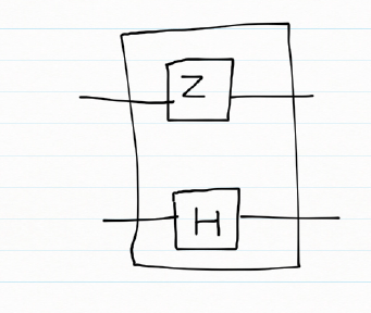
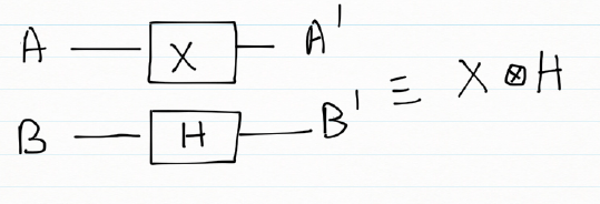
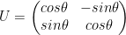
 and H =


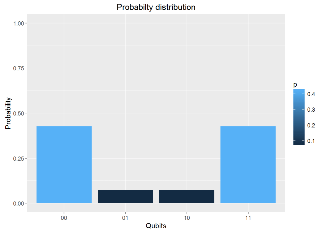
 possible configurations. However, at any