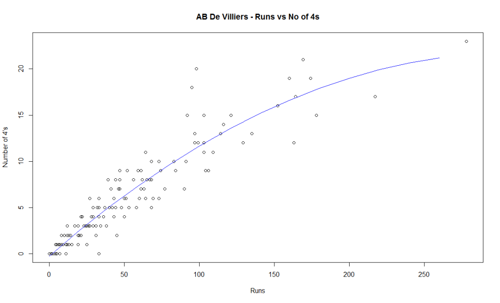
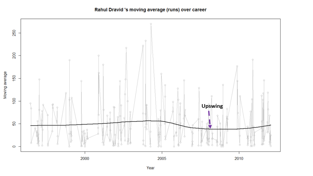
cricketr sizes up legendary All-rounders of yesteryear

Introduction

This is a post I have been wanting to write for several months, but had to put it off for one reason or another. In this post I use my R package cricketr to analyze the performance of All-rounder greats namely Kapil Dev, Ian Botham, Imran Khan and Richard Hadlee. All these players had talent that was natural and raw. They were good strikers of the ball and extremely lethal with their bowling. The ODI data for these players have been taken from ESPN Cricinfo.

Please be mindful of the ESPN Cricinfo Terms of Use

If you are passionate about cricket, and love analyzing cricket performances, then check out my racy book on cricket ‘Cricket analytics with cricketr and cricpy – Analytics harmony with R & Python’! This book discusses and shows how to use my R package ‘cricketr’ and my Python package ‘cricpy’ to analyze batsmen and bowlers in all formats of the game (Test, ODI and T20). The paperback is available on Amazon at $21.99 and the kindle version at $9.99/Rs 449/-. A must read for any cricket lover! Check it out!!

You can download the latest PDF version of the book at ‘Cricket analytics with cricketr and cricpy: Analytics harmony with R and Python-6th edition‘

Untitled

You can also read this post at Rpubs as cricketr-AR. Dowload this report as a PDF file from cricketr-AR

Important note 1: The latest release of ‘cricketr’ now includes the ability to analyze performances of teams now!! See Cricketr adds team analytics to its repertoire!!!

Important note 2 : Cricketr can now do a more fine-grained analysis of players, see Cricketr learns new tricks : Performs fine-grained analysis of players

Important note 3: Do check out the python avatar of cricketr, ‘cricpy’ in my post ‘Introducing cricpy:A python package to analyze performances of cricketers”

Note: If you would like to do a similar analysis for a different set of batsman and bowlers, you can clone/download my skeleton cricketr template from Github (which is the R Markdown file I have used for the analysis below). You will only need to make appropriate changes for the players you are interested in. Just a familiarity with R and R Markdown only is needed.

Important note: Do check out my other posts using cricketr at cricketr-posts

All Rounders

Kapil Dev (Ind)
Ian Botham (Eng)
Imran Khan (Pak)
Richard Hadlee (NZ)

I have sprinkled the plots with a few of my comments. Feel free to draw your conclusions! The analysis is included below

if (!require("cricketr")){ 
    install.packages("cricketr",) 
} 

library(cricketr)

The data for any particular ODI player can be obtained with the getPlayerDataOD() function. To do you will need to go to ESPN CricInfo Playerand type in the name of the player for e.g Kapil Dev, etc. This will bring up a page which have the profile number for the player e.g. for Kapil Dev this would be http://www.espncricinfo.com/india/content/player/30028.html. Hence, Kapils’s profile is 30028. This can be used to get the data for Kapil Dev’s data as shown below. I have already executed the below 4 commands and I will use the files to run further commands

#kapil1 
#botham11 
#imran1 
#hadlee1

Analyses of batting performances of the All Rounders

The following plots gives the analysis of the 4 ODI batsmen

Kapil Dev (Ind) – Innings – 225, Runs = 3783, Average=23.79, Strike Rate= 95.07
Ian Botham (Eng) – Innings – 116, Runs= 2113, Average=23.21, Strike Rate= 79.10
Imran Khan (Pak) – Innings – 175, Runs= 3709, Average=33.41, Strike Rate= 72.65
Richard Hadlee (NZ) – Innings – 115, Runs= 1751, Average=21.61, Strike Rate= 75.50

Plot of 4s, 6s and the scoring rate in ODIs

The 3 charts below give the number of

4s vs Runs scored
6s vs Runs scored
Balls faced vs Runs scored

A regression line is fitted in each of these plots for each of the ODI batsmen

A. Kapil Dev
It can be seen that Kapil scores four 4’s when he scores 50. Also after facing 50 deliveries he scores around 43

par(mfrow=c(1,3))
par(mar=c(4,4,2,2))
batsman4s("./kapil1.csv","Kapil")
batsman6s("./kapil1.csv","Kapil")
batsmanScoringRateODTT("./kapil1.csv","Kapil")

dev.off()

## null device 
##           1

B. Ian Botham
Botham scores around 39 runs after 50 deliveries

par(mfrow=c(1,3))
par(mar=c(4,4,2,2))
batsman4s("./botham1.csv","Botham")
batsman6s("./botham1.csv","Botham")
batsmanScoringRateODTT("./botham1.csv","Botham")

dev.off()

## null device 
##           1

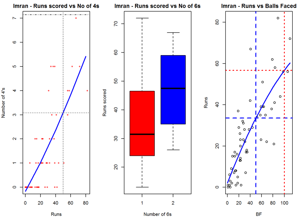
C. Imran Khan
Imran scores around 36 runs for 50 deliveries

par(mfrow=c(1,3))
par(mar=c(4,4,2,2))
batsman4s("./imran1.csv","Imran")
batsman6s("./imran1.csv","Imran")
batsmanScoringRateODTT("./imran1.csv","Imran")

dev.off()

## null device 
##           1

D. Richard Hadlee
Hadlee also scores around 30 runs facing 50 deliveries

par(mfrow=c(1,3))
par(mar=c(4,4,2,2))
batsman4s("./hadlee1.csv","Hadlee")
batsman6s("./hadlee1.csv","Hadlee")
batsmanScoringRateODTT("./hadlee1.csv","Hadlee")

dev.off()

## null device 
##           1

Cumulative Average runs of batsman in career

Kapils cumulative avrerage runs drops towards the last 15 innings wheres Botham had a good run towards the end of his career. Imran performance as a batsman really peaks towards the end with a cumulative average of almost 25 runs. Hadlee has a stead performance

par(mfrow=c(2,2))
par(mar=c(4,4,2,2))
batsmanCumulativeAverageRuns("./kapil1.csv","Kapil")

batsmanCumulativeAverageRuns("./botham1.csv","Botham")

batsmanCumulativeAverageRuns("./imran1.csv","Imran")

batsmanCumulativeAverageRuns("./hadlee1.csv","Hadlee")

dev.off()

## null device 
##           1

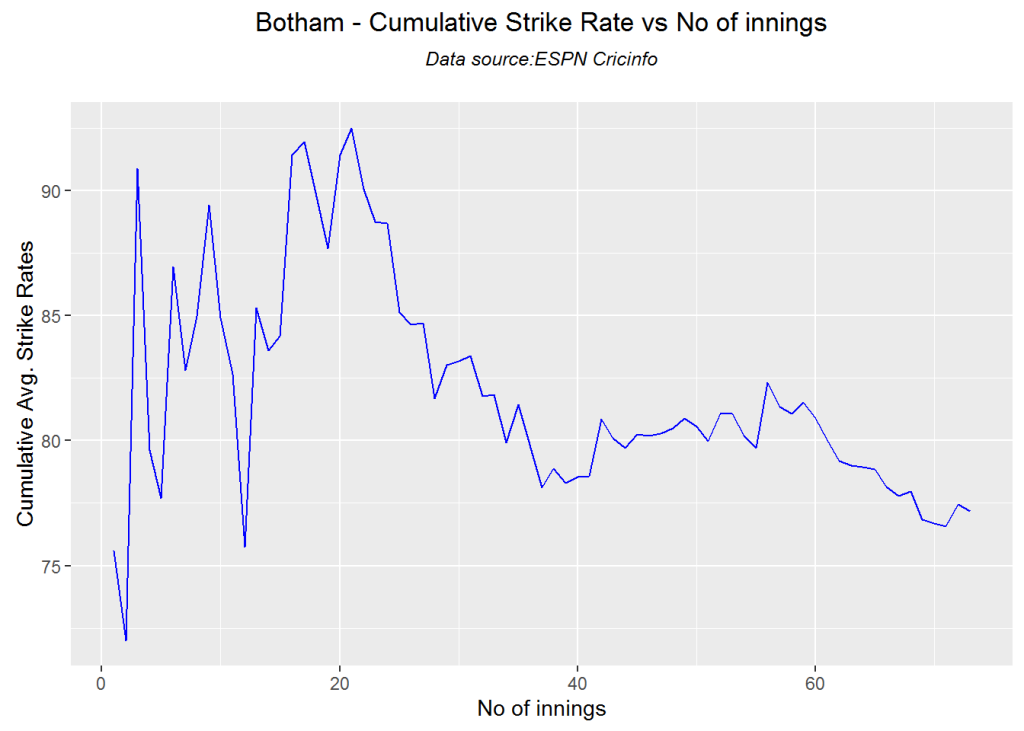
Cumulative Average strike rate of batsman in career

Kapil’s strike rate is superlative touching the 90’s steadily. Botham’s strike drops dramatically towards the latter part of his career. Imran average at a steady 75 and Hadlee averages around 85.

par(mfrow=c(2,2))
par(mar=c(4,4,2,2))
batsmanCumulativeStrikeRate("./kapil1.csv","Kapil")

batsmanCumulativeStrikeRate("./botham1.csv","Botham")

batsmanCumulativeStrikeRate("./imran1.csv","Imran")

batsmanCumulativeStrikeRate("./hadlee1.csv","Hadlee")

dev.off()

## null device 
##           1

Relative Mean Strike Rate

Kapil tops the strike rate among all the all-rounders. This is really a revelation to me. This can also be seen in the original data in Kapil’s strike rate is at a whopping 95.07 in comparison to Botham, Inran and Hadlee who are at 79.1,72.65 and 75.50 respectively

par(mar=c(4,4,2,2))
frames <- list("./kapil1.csv","./botham1.csv","imran1.csv","hadlee1.csv")
names <- list("Kapil","Botham","Imran","Hadlee")
relativeBatsmanSRODTT(frames,names)

Relative Runs Frequency Percentage

This plot shows that Imran has a much better average runs scored over the other all rounders followed by Kapil

frames <- list("./kapil1.csv","./botham1.csv","imran1.csv","hadlee1.csv")
names <- list("Kapil","Botham","Imran","Hadlee")
relativeRunsFreqPerfODTT(frames,names)

Relative cumulative average runs in career

It can be seen clearly that Imran Khan leads the pack in cumulative average runs followed by Kapil Dev and then Botham

frames <- list("./kapil1.csv","./botham1.csv","imran1.csv","hadlee1.csv")
names <- list("Kapil","Botham","Imran","Hadlee")
relativeBatsmanCumulativeAvgRuns(frames,names)

Relative cumulative average strike rate in career

In the cumulative strike rate Hadlee and Kapil run a close race.

frames <- list("./kapil1.csv","./botham1.csv","imran1.csv","hadlee1.csv")
names <- list("Kapil","Botham","Imran","Hadlee")
relativeBatsmanCumulativeStrikeRate(frames,names)

Percent 4’s,6’s in total runs scored

The plot below shows the contrib

frames <- list("./kapil1.csv","./botham1.csv","imran1.csv","hadlee1.csv")
names <- list("Kapil","Botham","Imran","Hadlee")
runs4s6s <-batsman4s6s(frames,names)

print(runs4s6s)

##                Kapil Botham Imran Hadlee
## Runs(1s,2s,3s) 72.08  66.53 77.53  73.27
## 4s             21.98  25.78 17.61  21.08
## 6s              5.94   7.68  4.86   5.65

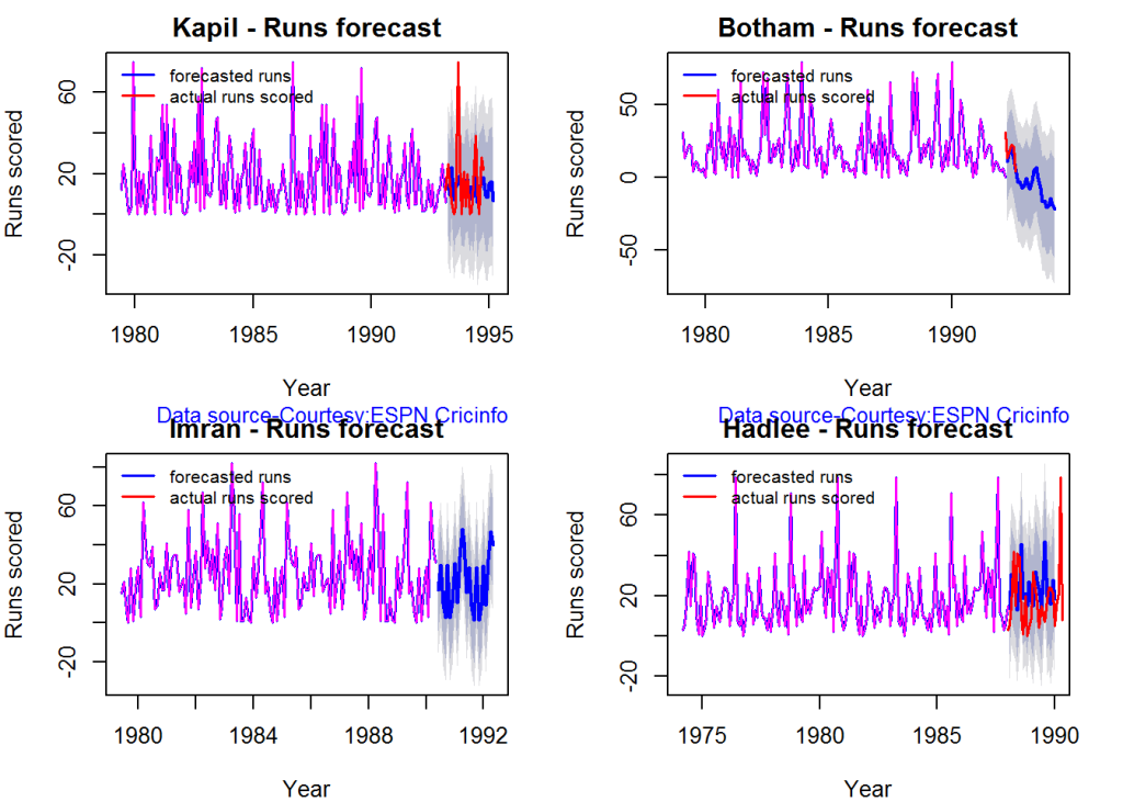
Runs forecast

The forecast for the batsman is shown below.

par(mfrow=c(2,2))
par(mar=c(4,4,2,2))
batsmanPerfForecast("./kapil1.csv","Kapil")
batsmanPerfForecast("./botham1.csv","Botham")
batsmanPerfForecast("./imran1.csv","Imran")

batsmanPerfForecast("./hadlee1.csv","Hadlee")

dev.off()

## null device 
##           1

3D plot of Runs vs Balls Faced and Minutes at Crease

The plot is a scatter plot of Runs vs Balls faced and Minutes at Crease. A prediction plane is fitted

par(mfrow=c(1,2))
par(mar=c(4,4,2,2))
battingPerf3d("./kapil1.csv","Kapil")
battingPerf3d("./botham1.csv","Botham")

dev.off()

## null device 
##           1

par(mfrow=c(1,2))
par(mar=c(4,4,2,2))
battingPerf3d("./imran1.csv","Imran")
battingPerf3d("./hadlee1.csv","Hadlee")

dev.off()

## null device 
##           1

Predicting Runs given Balls Faced and Minutes at Crease

A multi-variate regression plane is fitted between Runs and Balls faced +Minutes at crease.

BF <- seq( 10, 200,length=10)
Mins <- seq(30,220,length=10)
newDF <- data.frame(BF,Mins)

kapil <- batsmanRunsPredict("./kapil1.csv","Kapil",newdataframe=newDF)
botham <- batsmanRunsPredict("./botham1.csv","Botham",newdataframe=newDF)
imran <- batsmanRunsPredict("./imran1.csv","Imran",newdataframe=newDF)
hadlee <- batsmanRunsPredict("./hadlee1.csv","Hadlee",newdataframe=newDF)

The fitted model is then used to predict the runs that the batsmen will score for a hypotheticial Balls faced and Minutes at crease. It can be seen that Kapil is the best bet for a balls faced and minutes at crease followed by Botham.

batsmen <-cbind(round(kapil$Runs),round(botham$Runs),round(imran$Runs),round(hadlee$Runs))
colnames(batsmen) <- c("Kapil","Botham","Imran","Hadlee")
newDF <- data.frame(round(newDF$BF),round(newDF$Mins))
colnames(newDF) <- c("BallsFaced","MinsAtCrease")
predictedRuns <- cbind(newDF,batsmen)
predictedRuns

##    BallsFaced MinsAtCrease Kapil Botham Imran Hadlee
## 1          10           30    16      6    10     15
## 2          31           51    33     22    22     28
## 3          52           72    49     38    33     42
## 4          73           93    65     54    45     56
## 5          94          114    81     70    56     70
## 6         116          136    97     86    67     84
## 7         137          157   113    102    79     97
## 8         158          178   130    117    90    111
## 9         179          199   146    133   102    125
## 10        200          220   162    149   113    139

Highest runs likelihood

The plots below the runs likelihood of batsman. This uses K-Means . A. Kapil Dev

batsmanRunsLikelihood("./kapil1.csv","Kapil")

## Summary of  Kapil 's runs scoring likelihood
## **************************************************
## 
## There is a 34.57 % likelihood that Kapil  will make  22 Runs in  24 balls over 34  Minutes 
## There is a 17.28 % likelihood that Kapil  will make  46 Runs in  46 balls over  65  Minutes 
## There is a 48.15 % likelihood that Kapil  will make  5 Runs in  7 balls over 9  Minutes

B. Ian Botham

batsmanRunsLikelihood("./botham1.csv","Botham")

## Summary of  Botham 's runs scoring likelihood
## **************************************************
## 
## There is a 47.95 % likelihood that Botham  will make  9 Runs in  12 balls over 15  Minutes 
## There is a 39.73 % likelihood that Botham  will make  23 Runs in  32 balls over  44  Minutes 
## There is a 12.33 % likelihood that Botham  will make  59 Runs in  74 balls over 101  Minutes

C. Imran Khan

batsmanRunsLikelihood("./imran1.csv","Imran")

## Summary of  Imran 's runs scoring likelihood
## **************************************************
## 
## There is a 23.33 % likelihood that Imran  will make  36 Runs in  54 balls over 74  Minutes 
## There is a 60 % likelihood that Imran  will make  14 Runs in  18 balls over  23  Minutes 
## There is a 16.67 % likelihood that Imran  will make  53 Runs in  90 balls over 115  Minutes

D. Richard Hadlee

batsmanRunsLikelihood("./hadlee1.csv","Hadlee")

## Summary of  Hadlee 's runs scoring likelihood
## **************************************************
## 
## There is a 6.1 % likelihood that Hadlee  will make  64 Runs in  79 balls over 90  Minutes 
## There is a 42.68 % likelihood that Hadlee  will make  25 Runs in  33 balls over  44  Minutes 
## There is a 51.22 % likelihood that Hadlee  will make  9 Runs in  11 balls over 15  Minutes

Average runs at ground and against opposition

A. Kapil Dev

par(mfrow=c(1,2))
par(mar=c(4,4,2,2))
batsmanAvgRunsGround("./kapil1.csv","Kapil")
batsmanAvgRunsOpposition("./kapil1.csv","Kapil")

dev.off()

## null device 
##           1

B. Ian Botham

par(mfrow=c(1,2))
par(mar=c(4,4,2,2))
batsmanAvgRunsGround("./botham1.csv","Botham")
batsmanAvgRunsOpposition("./botham1.csv","Botham")

dev.off()

## null device 
##           1

C. Imran Khan

par(mfrow=c(1,2))
par(mar=c(4,4,2,2))
batsmanAvgRunsGround("./imran1.csv","Imran")
batsmanAvgRunsOpposition("./imran1.csv","Imran")

dev.off()

## null device 
##           1

D. Richard Hadlee

par(mfrow=c(1,2))
par(mar=c(4,4,2,2))
batsmanAvgRunsGround("./hadlee1.csv","Hadlee")
batsmanAvgRunsOpposition("./hadlee1.csv","Hadlee")

dev.off()

## null device 
##           1

Moving Average of runs over career

The moving average for the 4 batsmen indicate the following

Kapil’s performance drops significantly while there is a slump in Botham’s performance. On the other hand Imran and Hadlee’s performance were on the upswing.

par(mfrow=c(2,2))
par(mar=c(4,4,2,2))
batsmanMovingAverage("./kapil1.csv","Kapil")
batsmanMovingAverage("./botham1.csv","Botham")
batsmanMovingAverage("./imran1.csv","Imran")
batsmanMovingAverage("./hadlee1.csv","Hadlee")

dev.off()

## null device 
##           1

Check batsmen in-form, out-of-form

[1] “**************************** Form status of Kapil ****************************\n\n
Population size: 72
Mean of population: 19.38 \n
Sample size: 9 Mean of sample: 6.78 SD of sample: 6.14 \n\n
Null hypothesis H0 : Kapil ‘s sample average is within 95% confidence interval of population average\n
Alternative hypothesis Ha : Kapil ‘s sample average is below the 95% confidence interval of population average\n\n
Kapil ‘s Form Status: Out-of-Form because the p value: 8.4e-05 is less than alpha= 0.05

“**************************** Form status of Botham ****************************\n\n
Population size: 65
Mean of population: 21.29 \n
Sample size: 8 Mean of sample: 15.38 SD of sample: 13.19 \n\n
Null hypothesis H0 : Botham ‘s sample average is within 95% confidence interval of population average\n
Alternative hypothesis Ha : Botham ‘s sample average is below the 95% confidence interval of population average\n\n
Botham ‘s Form Status: In-Form because the p value: 0.120342 is greater than alpha= 0.05 \n

“**************************** Form status of Imran ****************************\n\n
Population size: 54
Mean of population: 24.94 \n
Sample size: 6 Mean of sample: 30.83 SD of sample: 25.4 \n\n
Null hypothesis H0 : Imran ‘s sample average is within 95% confidence interval of population average\n
Alternative hypothesis Ha : Imran ‘s sample average is below the 95% confidence interval of population average\n\n
Imran ‘s Form Status: In-Form because the p value: 0.704683 is greater than alpha= 0.05 \n

“**************************** Form status of Hadlee ****************************\n\n
Population size: 73
Mean of population: 18 \n
Sample size: 9 Mean of sample: 27 SD of sample: 24.27 \n\n
Null hypothesis H0 : Hadlee ‘s sample average is within 95% confidence interval of population average\n
Alternative hypothesis Ha : Hadlee ‘s sample average is below the 95% confidence interval of population average\n\n
Hadlee ‘s Form Status: In-Form because the p value: 0.85262 is greater than alpha= 0.05 \n *******************************************************************************************\n\n”

Analyses of bowling performances of the All Rounders

The following plots gives the analysis of the 4 ODI batsmen

Kapil Dev (Ind) – Innings – 225, Wickets = 253, Average=27.45, Economy Rate= 3.71
Ian Botham (Eng) – Innings – 116, Wickets = 145, Average=28.54, Economy Rate= 3.96
Imran Khan (Pak) – Innings – 175, Wickets = 182, Average=26.61, Economy Rate= 3.89
Richard Hadlee (NZ) – Innings – 115, Wickets = 158, Average=21.56, Economy Rate= 3.30

Botham has the highest number of innings and wickets followed closely by Mitchell. Imran and Hadlee have relatively fewer innings.

To get the bowler’s data use

#kapil2 
#botham2 
#imran2 
#hadlee2

“`

Wicket Frequency percentage

This plot gives the percentage of wickets for each wickets (1,2,3…etc).

par(mfrow=c(1,4))
par(mar=c(4,4,2,2))
bowlerWktsFreqPercent("./kapil2.csv","Kapil")
bowlerWktsFreqPercent("./botham2.csv","Botham")
bowlerWktsFreqPercent("./imran2.csv","Imran")
bowlerWktsFreqPercent("./hadlee2.csv","Hadlee")

dev.off()

## null device 
##           1

Wickets Runs plot

The plot below gives a boxplot of the runs ranges for each of the wickets taken by the bowlers.

par(mfrow=c(1,4))
par(mar=c(4,4,2,2))

bowlerWktsRunsPlot("./kapil2.csv","Kapil")
bowlerWktsRunsPlot("./botham2.csv","Botham")
bowlerWktsRunsPlot("./imran2.csv","Imran")
bowlerWktsRunsPlot("./hadlee2.csv","Hadlee")

dev.off()

## null device 
##           1

Cumulative average wicket plot

Botham has the best cumulative average wicket touching almost 1.6 wickets followed by Hadlee

par(mfrow=c(1,3))
par(mar=c(4,4,2,2))
bowlerCumulativeAvgWickets("./kapil2.csv","Kapil")

bowlerCumulativeAvgWickets("./botham2.csv","Botham")

bowlerCumulativeAvgWickets("./imran2.csv","Imran")

bowlerCumulativeAvgWickets("./hadlee2.csv","Hadlee")

dev.off()

## null device 
##           1

par(mfrow=c(1,3))
par(mar=c(4,4,2,2))
bowlerCumulativeAvgEconRate("./kapil2.csv","Kapil")

bowlerCumulativeAvgEconRate("./botham2.csv","Botham")

bowlerCumulativeAvgEconRate("./imran2.csv","Imran")

bowlerCumulativeAvgEconRate("./hadlee2.csv","Hadlee")

dev.off()

## null device 
##           1

Average wickets in different grounds and opposition

A. Kapil Dev

par(mfrow=c(1,2))
par(mar=c(4,4,2,2))
bowlerAvgWktsGround("./kapil2.csv","Kapil")
bowlerAvgWktsOpposition("./kapil2.csv","Kapil")

dev.off()

## null device 
##           1

B. Ian Botham

par(mfrow=c(1,2))
par(mar=c(4,4,2,2))
bowlerAvgWktsGround("./botham2.csv","Botham")
bowlerAvgWktsOpposition("./botham2.csv","Botham")

dev.off()

## null device 
##           1

C. Imran Khan

par(mfrow=c(1,2))
par(mar=c(4,4,2,2))
bowlerAvgWktsGround("./imran2.csv","Imran")
bowlerAvgWktsOpposition("./imran2.csv","Imran")

dev.off()

## null device 
##           1

D. Richard Hadlee

par(mfrow=c(1,2))
par(mar=c(4,4,2,2))
bowlerAvgWktsGround("./hadlee2.csv","Hadlee")
bowlerAvgWktsOpposition("./hadlee2.csv","Hadlee")

dev.off()

## null device 
##           1

Relative bowling performance

It can be seen that Botham is the most effective wicket taker of the lot

frames <- list("./kapil2.csv","./botham2.csv","imran2.csv","hadlee2.csv")
names <- list("Kapil","Botham","Imran","Hadlee")
relativeBowlingPerf(frames,names)

Relative Economy Rate against wickets taken

Hadlee has the best overall economy rate followed by Kapil Dev

frames <- list("./kapil2.csv","./botham2.csv","imran2.csv","hadlee2.csv")
names <- list("Kapil","Botham","Imran","Hadlee")
relativeBowlingERODTT(frames,names)

Relative cumulative average wickets of bowlers in career

This plot confirms the wicket taking ability of Botham followed by Hadlee

frames <- list("./kapil2.csv","./botham2.csv","imran2.csv","hadlee2.csv")
names <- list("Kapil","Botham","Imran","Hadlee")
relativeBowlerCumulativeAvgWickets(frames,names)

Relative cumulative average economy rate of bowlers

frames <- list("./kapil2.csv","./botham2.csv","imran2.csv","hadlee2.csv")
names <- list("Kapil","Botham","Imran","Hadlee")
relativeBowlerCumulativeAvgEconRate(frames,names)

Moving average of wickets over career

This plot shows that Hadlee has the best economy rate followed by Kapil

par(mfrow=c(2,2))
par(mar=c(4,4,2,2))
bowlerMovingAverage("./kapil2.csv","Kapil")
bowlerMovingAverage("./botham2.csv","Botham")
bowlerMovingAverage("./imran2.csv","Imran")
bowlerMovingAverage("./hadlee2.csv","Hadlee")

dev.off()

## null device 
##           1

Wickets forecast

par(mfrow=c(2,2))
par(mar=c(4,4,2,2))
bowlerPerfForecast("./kapil2.csv","Kapil")
bowlerPerfForecast("./botham2.csv","Botham")
bowlerPerfForecast("./imran2.csv","Imran")
bowlerPerfForecast("./hadlee2.csv","Hadlee")

dev.off()

## null device 
##           1

Check bowler in-form, out-of-form

“**************************** Form status of Kapil ****************************\n\n
Population size: 198
Mean of population: 1.2 \n Sample size: 23 Mean of sample: 0.65 SD of sample: 0.83 \n\n
Null hypothesis H0 : Kapil ‘s sample average is within 95% confidence interval \n of population average\n
Alternative hypothesis Ha : Kapil ‘s sample average is below the 95% confidence\n interval of population average\n\n
Kapil ‘s Form Status: Out-of-Form because the p value: 0.002097 is less than alpha= 0.05 \n

“**************************** Form status of Botham ****************************\n\n
Population size: 166
Mean of population: 1.58 \n Sample size: 19 Mean of sample: 1.47 SD of sample: 1.12 \n\n
Null hypothesis H0 : Botham ‘s sample average is within 95% confidence interval \n of population average\n
Alternative hypothesis Ha : Botham ‘s sample average is below the 95% confidence\n interval of population average\n\n
Botham ‘s Form Status: In-Form because the p value: 0.336694 is greater than alpha= 0.05 \n

“**************************** Form status of Imran ****************************\n\n
Population size: 137
Mean of population: 1.23 \n Sample size: 16 Mean of sample: 0.81 SD of sample: 0.91 \n\n
Null hypothesis H0 : Imran ‘s sample average is within 95% confidence interval \n of population average\n
Alternative hypothesis Ha : Imran ‘s sample average is below the 95% confidence\n interval of population average\n\n
Imran ‘s Form Status: Out-of-Form because the p value: 0.041727 is less than alpha= 0.05 \n

“**************************** Form status of Hadlee ****************************\n\n
Population size: 100
Mean of population: 1.38 \n Sample size: 12 Mean of sample: 1.67 SD of sample: 1.37 \n\n
Null hypothesis H0 : Hadlee ‘s sample average is within 95% confidence interval \n of population average\n
Alternative hypothesis Ha : Hadlee ‘s sample average is below the 95% confidence\n interval of population average\n\n
Hadlee ‘s Form Status: In-Form because the p value: 0.761265 is greater than alpha= 0.05 \n *******************************************************************************************\n\n”

Key findings

Here are some key conclusions ODI batsmen

Kapil Dev’s strike rate stands high above the other 3
Imran Khan has the best cumulative average runs followed by Kapil
Botham is the most effective wicket taker followed by Hadlee
Hadlee is the most economical bowler and is followed by Kapil Dev
For a hypothetical Balls Faced and Minutes at creases Kapil will score the most runs followed by Botham
The moving average of indicates that the best is yet to come for Imran and Hadlee. Kapil and Botham were on the decline

Also see my other posts in R

For a full list of posts see Index of posts

Sixer – R package cricketr’s new Shiny avatar

Published in R-bloggers: Sixer – R package cricketr’s new Shiny app

In this post I create a Shiny App, Sixer, based on my R package cricketr. I had developed the R package cricketr, a few months back for analyzing the performances of batsman and bowlers in all formats of the game (Test, ODI and Twenty 20). This package uses the statistics info available in ESPN Cricinfo Statsguru. I had written a series of posts using the cricketr package where I chose a few batsmen, bowlers and compared their performances of these players. Here I have created a complete Shiny app with a lot more players and with almost all the features of the cricketr package. The motivation for creating the Shiny app was to

To show case the ‘cricketr’ package and to highlight its functionalities
Perform analysis of more batsman and bowlers
Allow users to interact with the package and to allow them to try out the different features and functions of the package and to also check performances of some of their favorite crickets

Untitled

$4.99/Rs 320 and $6.99/Rs448 respectively

Important note 1: The latest release of ‘cricketr’ now includes the ability to analyze performances of teams now!! See Cricketr adds team analytics to its repertoire!!!

Important note 2 : Cricketr can now do a more fine-grained analysis of players, see Cricketr learns new tricks : Performs fine-grained analysis of players

Important note 3: Do check out the python avatar of cricketr, ‘cricpy’ in my post ‘Introducing cricpy:A python package to analyze performances of cricketers”

a) You can try out the interactive Shiny app Sixer at – Sixer
b) The code for this Shiny app project can be cloned/forked from GitHub – Sixer
Note: Please be mindful of ESPN Cricinfo Terms of Use.
(Take a look at my short video tutorial on my R package cricketr on Youtube – R package cricketr – A short tutorial)

Important note: Do check out my other posts using cricketr at cricketr-posts

In this Shiny app I have 5 tabs which perform the following function
1. Analyze Batsman
This tab analyzes batsmen based on different functions and plots the performances of the selected batsman. There are functions that compute and display batsman’s run-frequency ranges, Mean Strike rate, No of 4’s, dismissals, 3-D plot of Runs scored vs Balls Faced and Minutes at crease, Contribution to wins & losses, Home-Away record etc. The analyses can be done for Test cricketers, ODI and Twenty 20 batsman. I have included most of the Test batting giants including Tendulkar, Dravid, Sir Don Bradman, Viv Richards, Lara, Ponting etc. Similarly the ODI list includes Sehwag, Devilliers, Afridi, Maxwell etc. The Twenty20 list includes the Top 10 Twenty20 batsman based on their ICC rankings

2. Analyze bowler
This tab analyzes the bowling performances of bowlers, Wickets percentages, Mean Economy Rate, Wickets at different venues, Moving average of wickets etc. As earlier I have all the Top bowlers including Warne, Muralidharan, Kumble- the famed Indian spin quartet of Bedi, Chandrasekhar, Prasanna, Venkatraghavan, the deadly West Indies trio of Marshal, Roberts and Holding and the lethal combination of Imran Khan, Wasim Akram and Waqar Younis besides the dangerous Dennis Lillee and Jeff Thomson. Do give the functions a try and see for yourself the performances of these individual bowlers

3. Relative performances of batsman
This tab allows the selection of multiple batsmen (Test, ODI and Twenty 20) for comparisons. There are 2 main functions Relative Runs Frequency performance and Relative Mean Strike Rate

4. Relative performances of bowlers
Here we can compare bowling performances of multiple bowlers, which include functions Relative Bowling Performance and Relative Economy Rate. This can be done for Test, ODI and Twenty20 formats

5. Check for In-Form status of players
This tab checks the form status of batsman or bowler selected for all of the different formats of the game. The below computation uses Null Hypothesis testing and p-value to determine if the batsman is in-form or out-of-form. For this 90% of the career runs is chosen as the population and the mean computed. The last 10% is chosen to be the sample set and the sample Mean and the sample Standard Deviation are calculated. Note: The accuracy of the p-value test depends on the size of the population and the size of the sample set. It may not be very significant for players with a few innings played.

Some of my earlier posts based my R package cricketr are listed below
1. Introducing cricketr!: An R package for analyzing performances of cricketers
2. Taking cricketr for a spin – Part 1
3. cricketr plays the ODIs
4. cricketr adapts to the Twenty20 International
5. cricketr digs the Ashes

Do try out the interactive Sixer Shiny app – Sixer
You can clone the code from Github – Sixer

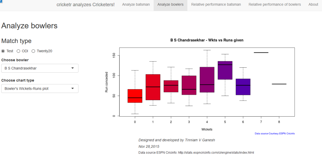
There is not much in way of explanation. The Shiny app’s use is self-explanatory. You can choose a match type ( Test,ODI or Twenty20), choose a batsman/bowler from the drop down list and select the plot you would like to seeHere a few sample plots
A. Analyze batsman tab
i) Batsman – Brian Lara , Match Type – Test, Function – Mean Strike Rate
ii) Batsman – Shahid Afridi, Match Type – ODI, Function – Runs vs Balls faced
The plot below shows that if Afridi faces around 50 balls he is likely to score around 60 runs in ODIs.
iii) Batsman – Chris Gayle, Match Type – Twenty20 Function – Moving Average
B. Analyze bowler tab

i. Bowler – B S Chandrasekhar, Match Type – Test, Function – Wickets vs Runs
ii) Bowler – Malcolm Marshall, Match Type – Test, Function – Mean Economy Rateiii) Bowler – Sunil Narine, Match Type – Twenty 20, Function – Bowler Wicket Rate

C. Relative performance of batsman (you can select more than 1)
The below plot gives the Mean Strike Rate of batsman. Viv Richards, Brian Lara, Sanath Jayasuriya and David Warner are best strikers of the ball.

Here are some of the great strikers of the ball in ODIs
D. Relative performance of bowlers (you can select more than 1)
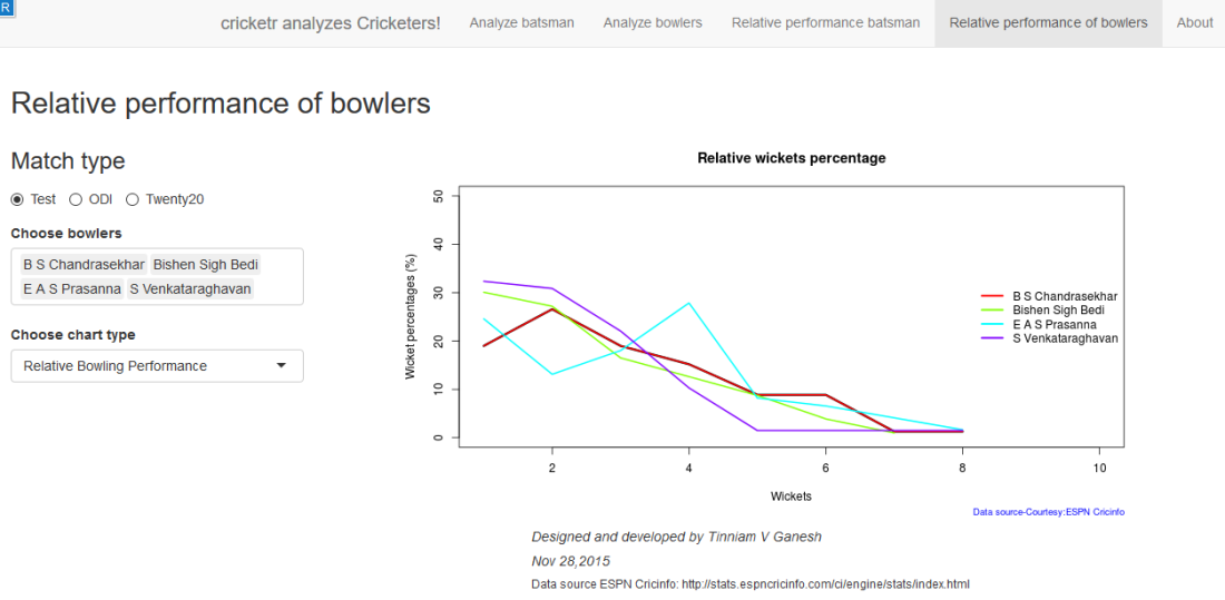
Finally a look at the famed Indian spin quartet. From the plot below it can be seen that B S Bedi & Venkatraghavan were more economical than Chandrasekhar and Prasanna.

But the latter have a better 4-5 wicket haul than the former two as seen in the plot below

Finally a look at the average number of balls to take a wicket by the Top 4 Twenty 20 bowlers.

E. Check for In-form status of players
Note: The accuracy of the p-value depends on the size of the population and the size of the sample set. It may not be very significant for smaller data sizes

i. Match Type – Test, Player Type – Batsman Name – Wickets v
In this plot the in-form status of Viv Richards is checked. This shows that Viv Richards was out-of-form
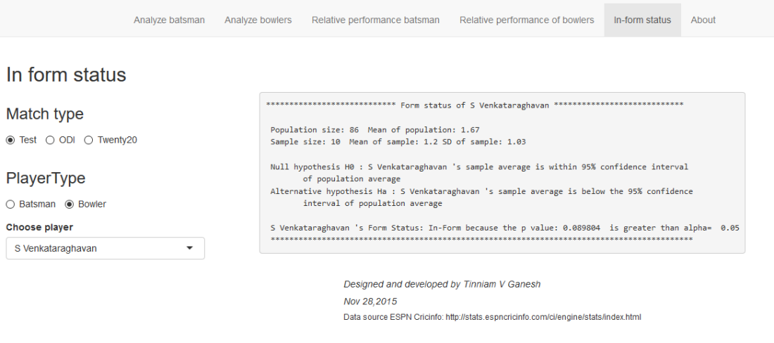
In the plot below the form status of S. Venkataraghavan is shown. According to this at the time of his retirement S Venkat was still in-form

Do give the Shiny app Sixer a try.

Also see
1. Literacy in India : A deepR dive.
2. Natural Language Processing: What would Shakespeare say?
3. Revisiting crimes against women in India
4. Informed choices through Machine Learning : Analyzing Kohli, Tendulkar and Dravid
5. Experiments with deblurring using OpenCV
6. What’s up Watson? Using IBM Watson’s QAAPI with Bluemix, NodeExpress – Part 1
7. Working with Node.js and PostgreSQL
8. A method for optimal bandwidth usage by auctioning available bandwidth using the OpenFlow Protocol
9. Latency, throughput implications for the cloud
10. A closer look at “Robot horse on a Trot! in Android”

cricketr adapts to the Twenty20 International!

Introduction

This should be last in the series of posts based on my R package cricketr. That is, unless some bright idea comes trotting along and light bulbs go on around my head.

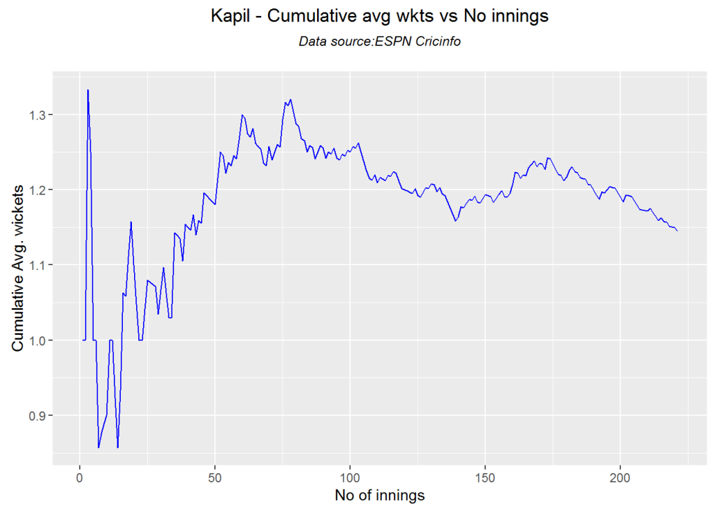
In this post cricketr adapts to the Twenty20 International format. Now cricketr can handle stats from all 3 formats of the game namely Test matches, ODIs and Twenty20 International from ESPN Cricinfo. You should be able to install the package from GitHub and use the many of the functions available in the package.

Please be mindful of the ESPN Cricinfo Terms of Use

You can download the latest PDF version of the book at ‘Cricket analytics with cricketr and cricpy: Analytics harmony with R and Python-6th edition‘

Untitled

Important note 1: The latest release of ‘cricketr’ now includes the ability to analyze performances of teams now!! See Cricketr adds team analytics to its repertoire!!!

Important note 2 : Cricketr can now do a more fine-grained analysis of players, see Cricketr learns new tricks : Performs fine-grained analysis of players

Important note 3: Do check out the python avatar of cricketr, ‘cricpy’ in my post ‘Introducing cricpy:A python package to analyze performances of cricketers”

You can also read this post at Rpubs as twenty20-cricketr. Download this report as a PDF file from twenty20-cricketr.pdf

Do check out my interactive Shiny app implementation using the cricketr package – Sixer – R package cricketr’s new Shiny avatar

Important note: Do check out my other posts using cricketr at cricketr-posts

I have chosen the Top 4 batsmen and top 4 bowlers based on ICC rankings and/or number of matches played.

Batsmen

Virat Kohli (Ind)
Faf du Plessis (SA)
A J Finch (Aus)
Brendon McCullum (Aus)

Bowlers

Samuel Badree (WI)
Sunil Narine (WI)
Ravichander Ashwin (Ind)
Ajantha Mendis (SL)

I have explained the plots and added my own observations. Please feel free to draw your conclusions!

The data for a particular player can be obtained with the getPlayerData() function. To do you will need to go to ESPN CricInfo Player and type in the name of the player for e.g Virat Kohli, Sunil Narine etc. This will bring up a page which have the profile number for the player e.g. for Virat Kohli this would be http://www.espncricinfo.com/india/content/player/253802.html.

The package can be installed directly from CRAN

if (!require("cricketr")){ 
    install.packages("cricketr",lib = "c:/test") 
} 
library(cricketr)

or from Github

library(devtools)
install_github("tvganesh/cricketr")
library(cricketr)

kohli <- getPlayerDataTT(253802,dir="..",file="kohli.csv",type="batting")

The analysis is included below

Analyses of Batsmen

The following plots gives the analysis of the 4 ODI batsmen

Virat Kohli (Ind) – Innings-26, Runs-972, Average-46.28,Strike Rate-131.70
Faf du Plessis (SA) – Innings-24, Runs-805, Average-42.36,Strike Rate-135.75
A J Finch (Aus) – Innings-22, Runs-756, Average-39.78,Strike Rate-152.41
Brendon McCullum (NZ) – Innings-70, Runs-2140, Average-35.66,Strike Rate-136.21

Plot of 4s, 6s and the scoring rate in ODIs

The 3 charts below give the number of

4s vs Runs scored
6s vs Runs scored
Balls faced vs Runs scored A regression line is fitted in each of these plots for each of the ODI batsmen

A. Virat Kohli
– The 1st plot shows that Kohli approximately hits about 5 4’s on his way to the 50s
– The 2nd box plot of no of 6s and runs shows the range of runs when Kohli scored 1,2 or 4 6s. The dark line in the box shows the average runs when he scored those number of 6s. So when he scored 1 6 the average runs he scored was 45
– The 3rd plot shows the number of runs scored against the balls faced. It can be seen when Kohli faced 50 balls he had scored around ~ 70 runs

par(mfrow=c(1,3))
par(mar=c(4,4,2,2))
batsman4s("./kohli.csv","Kohli")
batsman6s("./kohli.csv","Kohli")
batsmanScoringRateODTT("./kohli.csv","Kohli")

dev.off()

## null device 
##           1

B. Faf du Plessis

par(mfrow=c(1,3))
par(mar=c(4,4,2,2))
batsman4s("./plessis.csv","Du Plessis")
batsman6s("./plessis.csv","Du Plessis")
batsmanScoringRateODTT("./plessis.csv","Du Plessss")

dev.off()

## null device 
##           1

C. A J Finch

par(mfrow=c(1,3))
par(mar=c(4,4,2,2))
batsman4s("./finch.csv","A J Finch")
batsman6s("./finch.csv","A J Finch")
batsmanScoringRateODTT("./finch.csv","A J Finch")

dev.off()

## null device 
##           1

D. Brendon McCullum

par(mfrow=c(1,3))
par(mar=c(4,4,2,2))
batsman4s("./mccullum.csv","McCullum")
batsman6s("./mccullum.csv","McCullum")
batsmanScoringRateODTT("./mccullum.csv","McCullum")

dev.off()

## null device 
##           1

Relative Mean Strike Rate

This plot shows the Mean Strike Rate of the batsman in each run range. It can be seen the A J Finch has the best strike rate followed by B McCullum.

par(mar=c(4,4,2,2))
frames <- list("./kohli.csv","./plessis.csv","finch.csv","mccullum.csv")
names <- list("Kohli","Du Plessis","Finch","McCullum")
relativeBatsmanSRODTT(frames,names)

Relative Runs Frequency Percentage

The plot below provides the average runs scored in each run range 0-5,5-10,10-15 etc. Clearly Kohli has the most runs scored in most of the runs ranges. . This is also evident in the fact that Kohli has the highest average. He is followed by McCullum

frames <- list("./kohli.csv","./plessis.csv","finch.csv","mccullum.csv")
names <- list("Kohli","Du Plessis","Finch","McCullum")
relativeRunsFreqPerfODTT(frames,names)

Percent 4’s,6’s in total runs scored

The plot below shows the percentage of runs scored by way of 4s and 6s for each batsman. Du Plessis has the highest percentage of 4s, McCullum has the highest 6s. Finch has the highest percentage of 4s & 6s – 25.37 + 15.64= 41.01%

rames <- list("./kohli.csv","./plessis.csv","finch.csv","mccullum.csv")
names <- list("Kohli","Du Plessis","Finch","McCullum")
runs4s6s <-batsman4s6s(frames,names)

print(runs4s6s)

##                Kohli Du Plessis Finch McCullum
## Runs(1s,2s,3s) 64.29      64.55 58.99    61.45
## 4s             27.78      24.38 25.37    22.87
## 6s              7.94      11.07 15.64    15.69

3D plot of Runs vs Balls Faced and Minutes at Crease

The plot is a scatter plot of Runs vs Balls faced and Minutes at Crease. A prediction plane is then fitted based on the Balls Faced and Minutes at Crease to give the runs scored

par(mfrow=c(1,2))
par(mar=c(4,4,2,2))
battingPerf3d("./kohli.csv","Kohli")
battingPerf3d("./plessis.csv","Du Plessis")

dev.off()

## null device 
##           1

par(mfrow=c(1,2))
par(mar=c(4,4,2,2))
battingPerf3d("./finch.csv","A J Finch")
battingPerf3d("./mccullum.csv","McCullum")

dev.off()

## null device 
##           1

Predicting Runs given Balls Faced and Minutes at Crease

A hypothetical Balls faced and Minutes at Crease is used to predict the runs scored by each batsman based on the computed prediction plane

BF <- seq( 5, 70,length=10)
Mins <- seq(5,70,length=10)
newDF <- data.frame(BF,Mins)

kohli <- batsmanRunsPredict("./kohli.csv","Kohli",newdataframe=newDF)
plessis <- batsmanRunsPredict("./plessis.csv","Du Plessis",newdataframe=newDF)
finch <- batsmanRunsPredict("./finch.csv","A J Finch",newdataframe=newDF)
mccullum <- batsmanRunsPredict("./mccullum.csv","McCullum",newdataframe=newDF)

The predicted runs is displayed. As can be seen Finch has the best overall strike rate followed by McCullum.

batsmen <-cbind(round(kohli$Runs),round(plessis$Runs),round(finch$Runs),round(mccullum$Runs))
colnames(batsmen) <- c("Kohli","Du Plessis","Finch","McCullum")
newDF <- data.frame(round(newDF$BF),round(newDF$Mins))
colnames(newDF) <- c("BallsFaced","MinsAtCrease")
predictedRuns <- cbind(newDF,batsmen)
predictedRuns

##    BallsFaced MinsAtCrease Kohli Du Plessis Finch McCullum
## 1           5            5     2          1     5        3
## 2          12           12    12         10    22       16
## 3          19           19    22         19    40       28
## 4          27           27    31         28    57       41
## 5          34           34    41         37    74       54
## 6          41           41    51         47    91       66
## 7          48           48    60         56   108       79
## 8          56           56    70         65   125       91
## 9          63           63    79         74   142      104
## 10         70           70    89         84   159      117

Highest runs likelihood

The plots below the runs likelihood of batsman. This uses K-Means Kohli has the highest likelihood of scoring runs 34.2% likely to score 66 runs. Du Plessis has 25% likelihood to score 53 runs, A. Virat Kohli

batsmanRunsLikelihood("./kohli.csv","Kohli")

## Summary of  Kohli 's runs scoring likelihood
## **************************************************
## 
## There is a 23.08 % likelihood that Kohli  will make  10 Runs in  10 balls over 13  Minutes 
## There is a 42.31 % likelihood that Kohli  will make  29 Runs in  23 balls over  30  Minutes 
## There is a 34.62 % likelihood that Kohli  will make  66 Runs in  47 balls over 63  Minutes

B. Faf Du Plessis

batsmanRunsLikelihood("./plessis.csv","Du Plessis")

## Summary of  Du Plessis 's runs scoring likelihood
## **************************************************
## 
## There is a 62.5 % likelihood that Du Plessis  will make  14 Runs in  11 balls over 19  Minutes 
## There is a 25 % likelihood that Du Plessis  will make  53 Runs in  40 balls over  50  Minutes 
## There is a 12.5 % likelihood that Du Plessis  will make  94 Runs in  61 balls over 90  Minutes

C. A J Finch

batsmanRunsLikelihood("./finch.csv","A J Finch")

## Summary of  A J Finch 's runs scoring likelihood
## **************************************************
## 
## There is a 20 % likelihood that A J Finch  will make  95 Runs in  54 balls over 70  Minutes 
## There is a 25 % likelihood that A J Finch  will make  42 Runs in  27 balls over  35  Minutes 
## There is a 55 % likelihood that A J Finch  will make  8 Runs in  8 balls over 12  Minutes

D. Brendon McCullum

batsmanRunsLikelihood("./mccullum.csv","McCullum")

## Summary of  McCullum 's runs scoring likelihood
## **************************************************
## 
## There is a 50.72 % likelihood that McCullum  will make  11 Runs in  10 balls over 13  Minutes 
## There is a 28.99 % likelihood that McCullum  will make  36 Runs in  27 balls over  37  Minutes 
## There is a 20.29 % likelihood that McCullum  will make  74 Runs in  48 balls over 70  Minutes

Moving Average of runs over career

The moving average for the 4 batsmen indicate the following. It must be noted that there is not sufficient data yet on Twenty20 Internationals. Kpohli, Du Plessis and Finch average only 26 innings while McCullum has close to 70. So the moving average while an indication will regress towards the mean over time.

The moving average of Kohli and Du Plessis is on the way up.
McCullum has a consistent performance while Finch had a brief burst in 2013-2014

par(mfrow=c(2,2))
par(mar=c(4,4,2,2))
batsmanMovingAverage("./kohli.csv","Kohli")
batsmanMovingAverage("./plessis.csv","Du Plessis")
batsmanMovingAverage("./finch.csv","A J Finch")
batsmanMovingAverage("./mccullum.csv","McCullum")

dev.off()

## null device 
##           1

Analysis of bowlers

Samuel Badree (WI) – Innings-22, Runs -464, Wickets – 31, Econ Rate : 5.39
Sunil Narine (WI)- Innings-31,Runs-666, Wickets – 38 , Econ Rate : 5.70
Ravichander Ashwin (Ind)- Innings-26, Runs- 732, Wickets – 25, Econ Rate : 7.32
Ajantha Mendis (SL)- Innings-39, Runs – 952,Wickets – 66, Econ Rate : 6.45

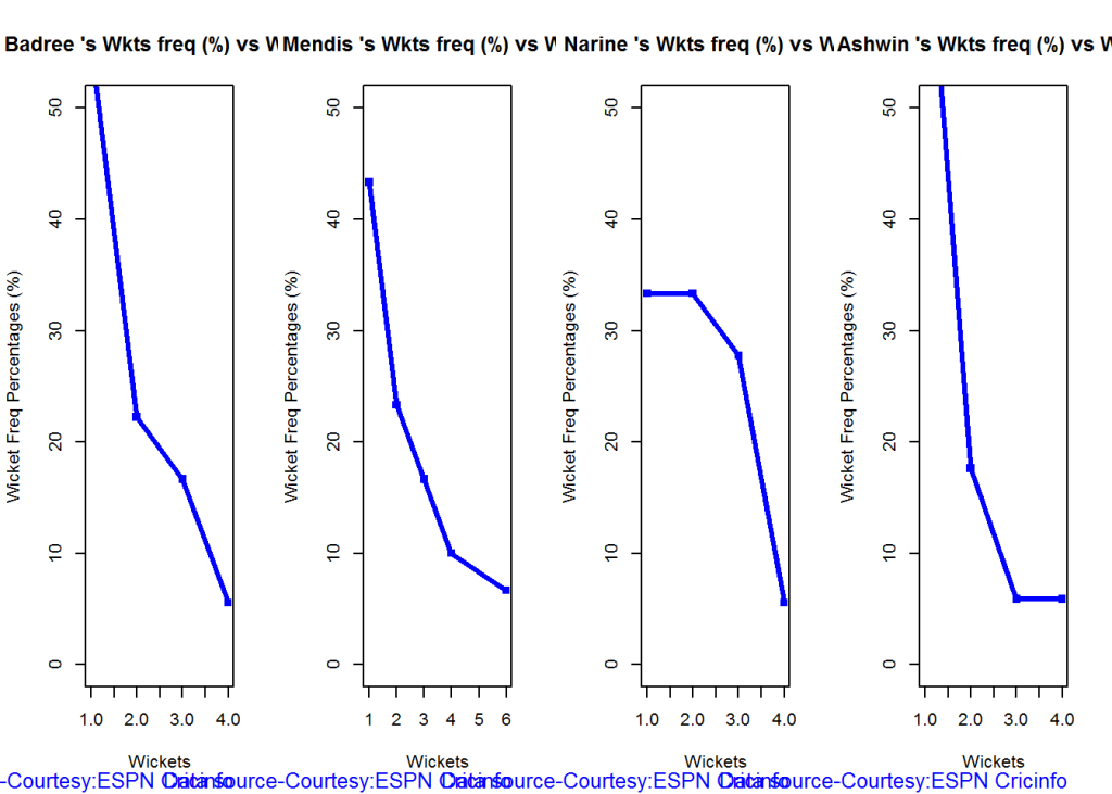
The plot shows the frequency with which the bowlers have taken 1,2,3 etc wickets. The most wickets taken is by Ajantha Mendis (6 wickets)

Wicket Frequency percentage

This plot gives the percentage of wickets for each wickets (1,2,3…etc)

par(mfrow=c(1,4))
par(mar=c(4,4,2,2))
bowlerWktsFreqPercent("./badree.csv","Badree")
bowlerWktsFreqPercent("./mendis.csv","Mendis")
bowlerWktsFreqPercent("./narine.csv","Narine")
bowlerWktsFreqPercent("./ashwin.csv","Ashwin")

dev.off()

## null device 
##           1

Wickets Runs plot

The plot below gives a boxplot of the runs ranges for each of the wickets taken by the bowlers. The ends of the box indicate the 25% and 75% percentile of runs scored for the wickets taken and the dark balck line is the average runs conceded.

par(mfrow=c(1,4))
par(mar=c(4,4,2,2))
bowlerWktsRunsPlot("./badree.csv","Badree")
bowlerWktsRunsPlot("./mendis.csv","Mendis")
bowlerWktsRunsPlot("./narine.csv","Narine")
bowlerWktsRunsPlot("./ashwin.csv","Ashwin")

dev.off()

## null device 
##           1

This plot below shows the average number of deliveries needed by the bowler to take the wickets (1,2,3 etc)

par(mfrow=c(1,2))
par(mar=c(4,4,2,2))
bowlerWktRateTT("./badree.csv","Badree")
bowlerWktRateTT("./mendis.csv","Mendis")

dev.off()

## null device 
##           1

par(mfrow=c(1,2))
par(mar=c(4,4,2,2))
bowlerWktRateTT("./narine.csv","Narine")
bowlerWktRateTT("./ashwin.csv","Ashwin")

dev.off()

## null device 
##           1

Relative bowling performance

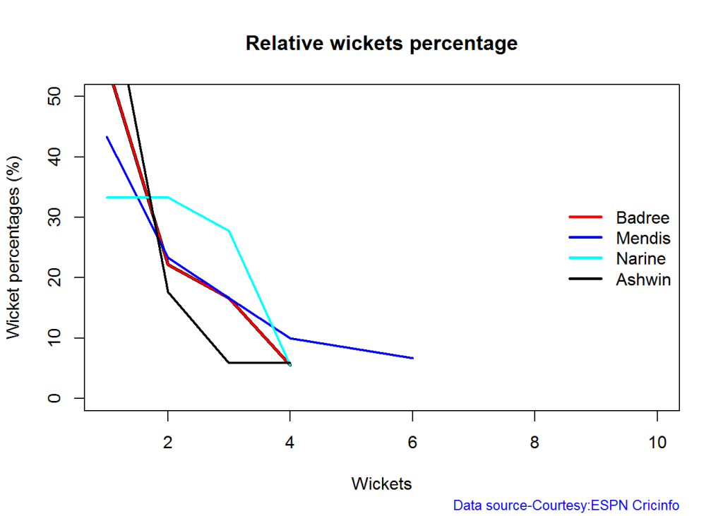
The plot below shows that Narine has the most wickets in the 2 -4 range followed by Mendis

frames <- list("./badree.csv","./mendis.csv","narine.csv","ashwin.csv")
names <- list("Badree","Mendis","Narine","Ashwin")
relativeBowlingPerf(frames,names)

Relative Economy Rate against wickets taken

The economy rate can be deduced as follows from the plot below. Narine has a good economy rate around 1 & 4 wickets, Ashwin around 2 wickets and Badree around 3. wickets

frames <- list("./badree.csv","./mendis.csv","narine.csv","ashwin.csv")
names <- list("Badree","Mendis","Narine","Ashwin")
relativeBowlingERODTT(frames,names)

Relative Wicket Rate

The relative wicket rate plots the mean number of deliveries needed to take the wickets namely (1,2,3,4). For e.g. Narine needed an average of 22 deliveries to take 1 wicket and 22.5,23.2, 24 deliveries to take 2,3 & 4 wickets respectively

frames <- list("./badree.csv","./mendis.csv","narine.csv","ashwin.csv")
names <- list("Badree","Mendis","Narine","Ashwin")
relativeWktRateTT(frames,names)

Moving average of wickets over career

par(mfrow=c(2,2))
par(mar=c(4,4,2,2))
bowlerMovingAverage("./badree.csv","Badree")
bowlerMovingAverage("./mendis.csv","Mendis")
bowlerMovingAverage("./narine.csv","Narine")
bowlerMovingAverage("./ashwin.csv","Ashwin")

## null device 
##           1

Key findings

Here are some key conclusions

Twenty 20 batsmen

Kohli has the a very consistent performance scoring high runs in the different run ranges. Kohli also has a 34.2% likelihood to score 6 runs. He is followed by McCullum for consisten performance
Finch has a best strike rate followed by McCullum.
Du Plessis has the highest percentage of 4s and McCullum has the percentage of 6s. Finch is superior in the percentage of runs scored in 4s and 6s
For a hypothetical balls faced and minutes at crease, Finch does best followed by McCullum
Kohli’s & Du Plessis Twenty20 career is on a upswing. Can they maintain the momentum. McCullum is consistent

Twenty20 bowlers

Narine has the highest wickets percentage for different wickets taken followed by Mendis
Mendis has taken 1,2,3,4,6 wickets in 24 deliveries
Narine has the lowest economy rate for 1 & 4 wickets, Ashwin for 2 wickets and Badree for 3 wickets. Mendis is comparatively expensive
Narine needed the least deliveries to get 1 (22.5) & 2 (23.2) wickets, Mendis needed 20.5 deliveries and Ashwin 19 deliveries for 4 wickets

Key takeaways 1. If all the above batsment and bowlers were in the same team we expect

Finch would be most useful when the run rate has to be greatly accelerated followed by McCullum
If the need is to consolidate, then Kohli is the best man for the job followed by McCullum
Overall McCullum is the best bet for Twenty20
When it comes to bowling Narine wins hands down as he has the most wickets, a good economy rate and a very good attack rate. So Narine is great bet for providing a vital breakthrough.

Also see my other posts in R

Taking cricketr for a spin – Part 1

“Curiouser and curiouser!” cried Alice
“The time has come,” the walrus said, “to talk of many things: Of shoes and ships – and sealing wax – of cabbages and kings”
“Begin at the beginning,”the King said, very gravely,“and go on till you come to the end: then stop.”
“And what is the use of a book,” thought Alice, “without pictures or conversation?”

            Excerpts from Alice in Wonderland by Lewis Carroll

Introduction

This post is a continuation of my previous post “Introducing cricketr! A R package to analyze the performances of cricketers.” In this post I take my package cricketr for a spin. For this analysis I focus on the Indian batting legends

– Sachin Tendulkar (Master Blaster)
– Rahul Dravid (The Will)
– Sourav Ganguly ( The Dada Prince)
– Sunil Gavaskar (Little Master)

This post is also hosted on RPubs – cricketr-1

If you are passionate about cricket, and love analyzing cricket performances, then check out my 2 racy books on cricket! In my books, I perform detailed yet compact analysis of performances of both batsmen, bowlers besides evaluating team & match performances in Tests , ODIs, T20s & IPL. You can buy my books on cricket from Amazon at $12.99 for the paperback and $4.99/$6.99 respectively for the kindle versions. The books can be accessed at Cricket analytics with cricketr and Beaten by sheer pace-Cricket analytics with yorkr A must read for any cricket lover! Check it out!!

You can download the latest PDF version of the book at ‘Cricket analytics with cricketr and cricpy: Analytics harmony with R and Python-6th edition‘

d $4.99/Rs 320 and $6.99/Rs448 respectively

Important note 1: The latest release of ‘cricketr’ now includes the ability to analyze performances of teams now!! See Cricketr adds team analytics to its repertoire!!!

Important note 2 : Cricketr can now do a more fine-grained analysis of players, see Cricketr learns new tricks : Performs fine-grained analysis of players

Important note 3: Do check out the python avatar of cricketr, ‘cricpy’ in my post ‘Introducing cricpy:A python package to analyze performances of cricketers”

(Do check out my interactive Shiny app implementation using the cricketr package – Sixer – R package cricketr’s new Shiny avatar)

The package can be installed directly from CRAN

if (!require("cricketr")){ 
    install.packages("cricketr",lib = "c:/test") 
} 
library(cricketr)

or from Github

library(devtools)
install_github("tvganesh/cricketr")
library(cricketr)

Box Histogram Plot

This plot shows a combined boxplot of the Runs ranges and a histogram of the Runs Frequency The plot below indicate the Tendulkar’s average is the highest. He is followed by Dravid, Gavaskar and then Ganguly

batsmanPerfBoxHist("./tendulkar.csv","Sachin Tendulkar")

batsmanPerfBoxHist("./dravid.csv","Rahul Dravid")

batsmanPerfBoxHist("./ganguly.csv","Sourav Ganguly")

batsmanPerfBoxHist("./gavaskar.csv","Sunil Gavaskar")

Relative Mean Strike Rate

In this first plot I plot the Mean Strike Rate of the batsmen. Tendulkar leads in the Mean Strike Rate for each runs in the range 100- 180. Ganguly has a very good Mean Strike Rate for runs range 40 -80

frames <- list("./tendulkar.csv","./dravid.csv","ganguly.csv","gavaskar.csv")
names <- list("Tendulkar","Dravid","Ganguly","Gavaskar")
relativeBatsmanSR(frames,names)

Relative Runs Frequency Percentage

The plot below show the percentage contribution in each 10 runs bucket over the entire career.The percentage Runs Frequency is fairly close but Gavaskar seems to lead most of the way

frames <- list("./tendulkar.csv","./dravid.csv","ganguly.csv","gavaskar.csv")
names <- list("Tendulkar","Dravid","Ganguly","Gavaskar")
relativeRunsFreqPerf(frames,names)

Moving Average of runs over career

The moving average for the 4 batsmen indicate the following – Tendulkar and Ganguly’s career has a downward trend and their retirement didn’t come too soon – Dravid and Gavaskar’s career definitely shows an upswing. They probably had a year or two left.

par(mfrow=c(2,2))
par(mar=c(4,4,2,2))
batsmanMovingAverage("./tendulkar.csv","Tendulkar")
batsmanMovingAverage("./dravid.csv","Dravid")
batsmanMovingAverage("./ganguly.csv","Ganguly")
batsmanMovingAverage("./gavaskar.csv","Gavaskar")

dev.off()

## null device 
##           1

Runs forecast

The forecast for the batsman is shown below. The plots indicate that only Tendulkar seemed to maintain a consistency over the period while the rest seem to score less than their forecasted runs in the last 10% of the career

par(mfrow=c(2,2))
par(mar=c(4,4,2,2))
batsmanPerfForecast("./tendulkar.csv","Sachin Tendulkar")
batsmanPerfForecast("./dravid.csv","Rahul Dravid")
batsmanPerfForecast("./ganguly.csv","Sourav Ganguly")
batsmanPerfForecast("./gavaskar.csv","Sunil Gavaskar")

dev.off()

## null device 
##           1

Check for batsman in-form/out-of-form

The following snippet checks whether the batsman is in-inform or ouyt-of-form during the last 10% innings of the career. This is done by choosing the null hypothesis (h0) to indicate that the batsmen are in-form. Ha is the alternative hypothesis that they are not-in-form. The population is based on the 1st 90% of career runs. The last 10% is taken as the sample and a check is made on the lower tail to see if the sample mean is less than 95% confidence interval. If this difference is >0.05 then the batsman is considered out-of-form.

The computation show that Tendulkar was out-of-form while the other’s weren’t. While Dravid and Gavaskar’s moving average do show an upward trend the surprise is Ganguly. This could be that Ganguly was able to keep his average in the last 10% to with the 95$ confidence interval. It has to be noted that Ganguly’s average was much lower than Tendulkar

checkBatsmanInForm("./tendulkar.csv","Tendulkar")

## *******************************************************************************************
## 
## Population size: 294  Mean of population: 50.48 
## Sample size: 33  Mean of sample: 32.42 SD of sample: 29.8 
## 
## Null hypothesis H0 : Tendulkar 's sample average is within 95% confidence interval 
##         of population average
## Alternative hypothesis Ha : Tendulkar 's sample average is below the 95% confidence
##         interval of population average
## 
## [1] "Tendulkar 's Form Status: Out-of-Form because the p value: 0.000713  is less than alpha=  0.05"
## *******************************************************************************************

checkBatsmanInForm("./dravid.csv","Dravid")

## *******************************************************************************************
## 
## Population size: 256  Mean of population: 46.98 
## Sample size: 29  Mean of sample: 43.48 SD of sample: 40.89 
## 
## Null hypothesis H0 : Dravid 's sample average is within 95% confidence interval 
##         of population average
## Alternative hypothesis Ha : Dravid 's sample average is below the 95% confidence
##         interval of population average
## 
## [1] "Dravid 's Form Status: In-Form because the p value: 0.324138  is greater than alpha=  0.05"
## *******************************************************************************************

checkBatsmanInForm("./ganguly.csv","Ganguly")

## *******************************************************************************************
## 
## Population size: 169  Mean of population: 38.94 
## Sample size: 19  Mean of sample: 33.21 SD of sample: 32.97 
## 
## Null hypothesis H0 : Ganguly 's sample average is within 95% confidence interval 
##         of population average
## Alternative hypothesis Ha : Ganguly 's sample average is below the 95% confidence
##         interval of population average
## 
## [1] "Ganguly 's Form Status: In-Form because the p value: 0.229006  is greater than alpha=  0.05"
## *******************************************************************************************

checkBatsmanInForm("./gavaskar.csv","Gavaskar")

## *******************************************************************************************
## 
## Population size: 125  Mean of population: 44.67 
## Sample size: 14  Mean of sample: 57.86 SD of sample: 58.55 
## 
## Null hypothesis H0 : Gavaskar 's sample average is within 95% confidence interval 
##         of population average
## Alternative hypothesis Ha : Gavaskar 's sample average is below the 95% confidence
##         interval of population average
## 
## [1] "Gavaskar 's Form Status: In-Form because the p value: 0.793276  is greater than alpha=  0.05"
## *******************************************************************************************

dev.off()

## null device 
##           1

3D plot of Runs vs Balls Faced and Minutes at Crease

The plot is a scatter plot of Runs vs Balls faced and Minutes at Crease. A prediction plane is fitted

par(mfrow=c(1,2))
par(mar=c(4,4,2,2))
battingPerf3d("./tendulkar.csv","Tendulkar")
battingPerf3d("./dravid.csv","Dravid")

par(mfrow=c(1,2))
par(mar=c(4,4,2,2))
battingPerf3d("./ganguly.csv","Ganguly")
battingPerf3d("./gavaskar.csv","Gavaskar")

dev.off()

## null device 
##           1

Predicting Runs given Balls Faced and Minutes at Crease

A multi-variate regression plane is fitted between Runs and Balls faced +Minutes at crease.

BF <- seq( 10, 400,length=15)
Mins <- seq(30,600,length=15)
newDF <- data.frame(BF,Mins)
tendulkar <- batsmanRunsPredict("./tendulkar.csv","Tendulkar",newdataframe=newDF)
dravid <- batsmanRunsPredict("./dravid.csv","Dravid",newdataframe=newDF)
ganguly <- batsmanRunsPredict("./ganguly.csv","Ganguly",newdataframe=newDF)
gavaskar <- batsmanRunsPredict("./gavaskar.csv","Gavaskar",newdataframe=newDF)

The fitted model is then used to predict the runs that the batsmen will score for a given Balls faced and Minutes at crease. It can be seen Tendulkar has a much higher Runs scored than all of the others.

Tendulkar is followed by Ganguly who we saw earlier had a very good strike rate. However it must be noted that Dravid and Gavaskar have a better average.

batsmen <-cbind(round(tendulkar$Runs),round(dravid$Runs),round(ganguly$Runs),round(gavaskar$Runs))
colnames(batsmen) <- c("Tendulkar","Dravid","Ganguly","Gavaskar")
newDF <- data.frame(round(newDF$BF),round(newDF$Mins))
colnames(newDF) <- c("BallsFaced","MinsAtCrease")
predictedRuns <- cbind(newDF,batsmen)
predictedRuns

##    BallsFaced MinsAtCrease Tendulkar Dravid Ganguly Gavaskar
## 1          10           30         7      1       7        4
## 2          38           71        23     14      21       17
## 3          66          111        39     27      35       30
## 4          94          152        54     40      50       43
## 5         121          193        70     54      64       56
## 6         149          234        86     67      78       69
## 7         177          274       102     80      93       82
## 8         205          315       118     94     107       95
## 9         233          356       134    107     121      108
## 10        261          396       150    120     136      121
## 11        289          437       165    134     150      134
## 12        316          478       181    147     165      147
## 13        344          519       197    160     179      160
## 14        372          559       213    173     193      173
## 15        400          600       229    187     208      186

Contribution to matches won and lost

par(mfrow=c(2,2))
par(mar=c(4,4,2,2))
batsmanContributionWonLost(35320,"Tendulkar")
batsmanContributionWonLost(28114,"Dravid")
batsmanContributionWonLost(28779,"Ganguly")
batsmanContributionWonLost(28794,"Gavaskar")

Home and overseas performance

From the plot below Tendulkar and Dravid have a lot more matches both home and abroad and their performance has good both at home and overseas. Tendulkar has the best performance home and abroad and is consistent all across. Dravid is also cossistent at all venues. Gavaskar played fewer matches than Tendulkar & Dravid. The range of runs at home is higher than overseas, however the average is consistent both at home and abroad. Finally we have Ganguly.

par(mfrow=c(2,2))
par(mar=c(4,4,2,2))
batsmanPerfHomeAway(35320,"Tendulkar")
batsmanPerfHomeAway(28114,"Dravid")
batsmanPerfHomeAway(28779,"Ganguly")
batsmanPerfHomeAway(28794,"Gavaskar")

Average runs at ground and against opposition

Tendulkar has above 50 runs average against Sri Lanka, Bangladesh, West Indies and Zimbabwe. The performance against Australia and England average very close to 50. Sydney, Port Elizabeth, Bloemfontein, Collombo are great huntings grounds for Tendulkar

par(mfrow=c(1,2))
par(mar=c(4,4,2,2))
batsmanAvgRunsGround("./tendulkar.csv","Tendulkar")
batsmanAvgRunsOpposition("./tendulkar.csv","Tendulkar")

dev.off()

## null device 
##           1

Dravid plundered runs at Adelaide, Georgetown, Oval, Hamiltom etc. Dravid has above average against England, Bangaldesh, New Zealand, Pakistan, West Indies and Zimbabwe

par(mfrow=c(1,2))
par(mar=c(4,4,2,2))
batsmanAvgRunsGround("./dravid.csv","Dravid")
batsmanAvgRunsOpposition("./dravid.csv","Dravid")

dev.off()

## null device 
##           1

Ganguly has good performance at the Oval, Rawalpindi, Johannesburg and Kandy. Ganguly averages 50 runs against England and Bangladesh.

par(mfrow=c(1,2))
par(mar=c(4,4,2,2))
batsmanAvgRunsGround("./ganguly.csv","Ganguly")
batsmanAvgRunsOpposition("./ganguly.csv","Ganguly")

dev.off()

## null device 
##           1

The Oval, Sydney, Perth, Melbourne, Brisbane, Manchester are happy hunting grounds for Gavaskar. Gavaskar averages around 50 runs Australia, Pakistan, Sri Lanka, West Indies.

par(mfrow=c(1,2))
par(mar=c(4,4,2,2))
batsmanAvgRunsGround("./gavaskar.csv","Gavaskar")
batsmanAvgRunsOpposition("./gavaskar.csv","Gavaskar")

dev.off()

## null device 
##           1

Key findings

Here are some key conclusions

Tendulkar has the highest average among the 4. He is followed by Dravid, Gavaskar and Ganguly.
Tendulkar’s predicted performance for a given number of Balls Faced and Minutes at Crease is superior to the rest
Dravid averages above 50 against 6 countries
West Indies and Australia are Gavaskar’s favorite batting grounds
Ganguly has a very good Mean Strike Rate for the range 40-80 and Tendulkar from 100-180
In home and overseas performance, Tendulkar is the best. Dravid and Gavaskar also have good performance overseas.
Dravid and Gavaskar probably retired a year or two earlier while Tendulkar and Ganguly’s time was clearly up

Final thoughts

Tendulkar is clearly the greatest batsman India has produced as he leads in almost all aspects of batting – number of centuries, strike rate, predicted runs and home and overseas performance. Dravid follows Tendulkar with 48 centuries, consistent performance home and overseas and a career that was still green. Gavaskar has fewer matches than rest but his performance overseas is very good in those helmetless times. Finally we have Ganguly.

Dravid and Gavaskar had a few more years of great batting while Tendulkar and Ganguly’s career was on a decline.

Note:It is really not fair to include Gavaskar in the analysis as he played in a different era when helmets were not used, even against the fiery pace of Thomson, Lillee, Roberts, Holding etc. In addition Gavaskar did not play against some of the newer countries like Bangladesh and Zimbabwe where he could have amassed runs. Yet I wanted to include him and his performance is clearly excellent

Also see my other posts in R

Analyzing cricket’s batting legends – Through the mirage with R

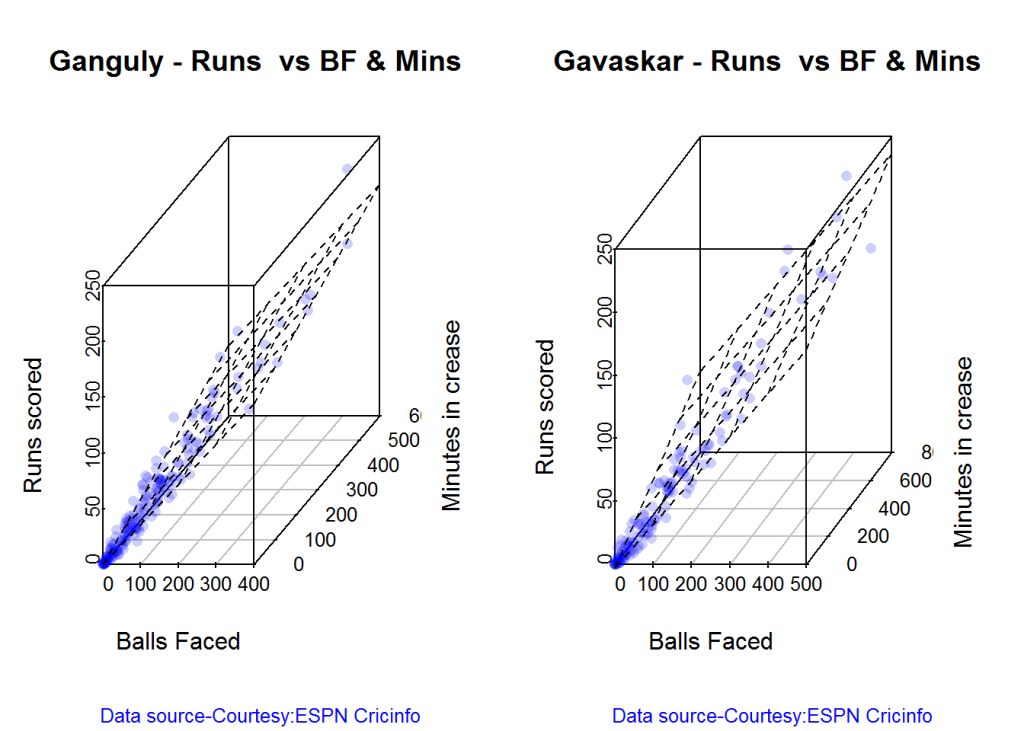
In this post I do a deep dive into the records of the all-time batting legends of cricket to identify interesting information about their achievements. In my opinion, the usual currency for batsman’s performance like most number of centuries or highest batting average are too gross in their significance. I wanted something finer where we can pin-point specific strengths of different players

This post will answer the following questions.
– How many times has a batsman scored runs in a specific range say 20-40 or 80-100 and so on?
– How do different batsmen compare against each other?
– Which of the batsmen stayed well beyond their sell-by date?
– Which of the batsmen retired too soon?
– What is the propensity for a batsman to get caught, bowled run out etc?

For this analysis I have chosen the batsmen below for the following reasons
Sir Don Bradman : With a batting average of 99.94 Bradman was an obvious choice
Sunil Gavaskar is one of India’s batting icons who amassed 774 runs in his debut against the formidable West Indies in West Indies
Brian Lara : A West Indian batting hero who has double, triple and quadruple centuries under his belt
Sachin Tendulkar: A prolific run getter, India’s idol, who holds the record for most test centuries by any batsman (51 centuries)
Ricky Ponting:A dangerous batsman against any bowling attack and who can demolish any bowler on his day
Rahul Dravid: He was India’s most dependable batsman who could weather any storm in a match single-handedly
AB De Villiers : The destructive South African batsman who can pulverize any attack when he gets going

The analysis has been performed on these batsmen on various parameters. Clearly different batsmen have shone in different batting aspects. The analysis focuses on each of these to see how the different players stack up against each other.

The data for the above batsmen has been taken from ESPN Cricinfo. Only the batting statistics of the above batsmen in Test cricket has been taken. The implementation for this analysis has been done using the R language. The R implementation, datasets and the plots can be accessed at GitHub at analyze-batting-legends. Feel free to fork or clone the code. You should be able to use the code with minor modifications on other players. Also go ahead make your own modifications and hack away!

Important note: Do check out the python avatar of cricketr, ‘cricpy’ in my post ‘Introducing cricpy:A python package to analyze performances of cricketers”

Key insights from my analysis below
a) Sir Don Bradman’s unmatchable record of 99.94 test average with several centuries, double and triple centuries makes him the gold standard of test batting as seen in the ‘All-time best batsman below’
b) Sunil Gavaskar is the king of batting in India, followed by Rahul Dravid and finally Sachin Tendulkar. See the charts below for details
c) Sunil Gavaskar and Rahul Dravid had at least 2 more years of good test cricket in them. Their retirement was premature. This is based on the individual batsmen’s career graph (moving average below)
d) Brian Lara, Sachin Tendulkar, Ricky Ponting, Vivian Richards retired at a time when their batting was clearly declining. The writing on the wall was clear and they had to go (see moving average below)
e) The biggest hitter of 4’s was Vivian Richards. In the 2nd place is Brian Lara. Tendulkar & Dravid follow behind. Dravid is a surprise as he has the image of a defender.
e) While Sir Don Bradman made huge scores, the number of 4’s in his innings was significantly less. This could be because the ground in those days did not carry the ball far enough
f) With respect to dismissals Richards was able to keep his wicket intact (11%) of the times , followed by Ponting Tendulkar, De Villiers, Dravid (10%) who carried the bat, and Gavaskar & Bradman (7%)

A) Runs frequency table and charts
These plots normalize the batting performance of different batsman, since the number of innings played ranges from 89 (Bradman) to 348 (Tendulkar), by calculating the percentage frequency the batsman scores runs in a particular range. For e.g. Sunil Gavaskar made scores between 60-80 10% of his total innings

This is shown in a tabular form below

The individual charts for each of the players are shwon belowThe top performers after removing ranges 0-20 & 20-40 are
Between 40-60 runs – 1) Ricky Ponting (16.4%) 2) Brian lara (15.8%) 3) AB De Villiers (14.6%)
Between 60-80 runs – 1) Vivian Richards (18%) 2) AB De Villiers (10.2%) 3) Sunil Gavaskar (10%)
Between 80-100 runs – 1) Rahul Dravid (7.6%) 2) Brian Lara (7.4%) 3) AB De Villiers (6.4%)
Between 100 -120 runs – 1) Sunil Gavaskar (7.5%) 2) Sir Don Bradman (6.8%) 3) Vivian Richards (5.8%)
Between 120-140 runs – 1) Sir Don Bradman (6.8%) 2) Sachin Tendulkar (2.5%) 3) Vivian Richards (2.3%)

The percentage frequency for Brian Lara is included below
1) Brian Lara

The above chart shows out of the total number of innings played by Brian Lara he scored runs in the range (40-60) 16% percent of the time. The chart also shows that Lara scored between 0-20, 40% while also scoring in the ranges 360-380 & 380-400 around 1%.
The same chart is displayed as continuous graph below

The run frequency charts for other batsman are
2) Sir Don Bradman
a) Run frequency

Note: Notice the significant contributions by Sir Don Bradman in the ranges 120-140,140-160,220-240,all the way up to 340
b) Performance

3) Sunil Gavaskar
a) Runs frequency chart

b) Performance chart

4) Sachin Tendulkar
a) Runs frequency chart

b) Performance chart

5) Ricky Ponting
a) Runs frequency

b) Performance

6) Rahul Dravid
a) Runs frequency chart

b) Performance chart

7) Vivian Richards
a) Runs frequency chart

b) Performance chart

8) AB De Villiers
a) Runs frequency chart

b) Performance chart

B) Relative performance of the players
In this section I try to measure the relative performance of the players by superimposing the performance graphs obtained above. You may say that “comparisons are odious!”. But equally odious are myths that are based on gross facts like highest runs, average or most number of centuries.
a) All-time best batsman
(Sir Don Bradman, Sunil Gavaskar, Vivian Richards, Sachin Tendulkar, Ricky Ponting, Brian Lara, Rahul Dravid, AB De Villiers)

From the above chart it is clear that Sir Don Bradman is the ‘gold’ standard in batting. He is well above others for run ranges above 100 – 350
b) Best Indian batsman (Sunil Gavaskar, Sachin Tendulkar, Rahul Dravid)

The above chart shows that Gavaskar is ahead of the other two for key ranges between 100 – 130 with almost 8% contribution of total runs. This followed by Dravid who is ahead of Tendulkar in the range 80-120. According to me the all time best Indian batsman is 1) Sunil Gavaskar 2) Rahul Dravid 3) Sachin Tendulkar

c) Best batsman -( Brian Lara, Ricky Ponting, Sachin Tendulkar, AB De Villiers)
This chart was prepared since this comparison was often made in recent times

This chart shows the following ranking 1) AB De Villiers 2) Sachin Tendulkar 3) Brian Lara/Ricky Ponting
C) Chart of 4’s

This chart is plotted with a 2nd order curve of the number of 4’s versus the total runs in the innings
1) Brian Lara

2) Sir Don Bradman

3) Sunil Gavaskar

4) Sachin Tendulkar

5) Ricky Ponting

6) Rahul Dravid

7) Vivian Richards

8) AB De Villiers

D) Proclivity for type of dismissal
The below charts show how often the batsman was out bowled, caught, run out etc
1) Brian Lara

2) Sir Don Bradman

3) Sunil Gavaskar

4) Sachin Tendulkar

5) Ricky Ponting

6) Rahul Dravid

7) Vivian Richard

8) AB De Villiers

E) Moving Average
The plots below provide the performance of the batsman as a time series (chronological) and is displayed as the continuous gray lines. A moving average is computed using ‘loess regression’ and is shown as the dark line. This dark line represents the players performance improvement or decline. The moving average plots are shown below
1) Brian Lara

2) Sir Don Bradman

Sir Don Bradman’s moving average shows a remarkably consistent performance over the years. He probably could have a continued for a couple more years
3)Sunil Gavaskar

Gavaskar moving average does show a good improvement from a dip around 1983. Gavaskar retired bowing to public pressure on a mistaken belief that he was under performing. Gavaskar could have a continued for a couple of more years
4) Sachin Tendulkar

Tendulkar’s performance is clearly on the decline from 2011. He could have announced his retirement at least 2 years prior
5) Ricky Ponting

Ponting peak performance was around 2005 and does go steeply downward from then on. Ponting could have also retired around 2012
6) Rahul Dravid

Dravid seems to have recovered very effectively from his poor for around 2009. His overall performance shows steady improvement. Dravid’s announcement appeared impulsive. Dravid had another 2 good years of test cricket in him
7) Vivian Richards

Richard’s performance seems to have dropped around 1984 and seems to remain that way.
8) AB De Villiers

AB De Villiers moving average shows a steady upward swing from 2009 onwards. De Villiers has at least 3-4 years of great test cricket ahead of him.

Finally as mentioned above the dataset, the R implementation and all the charts are available at GitHub at analyze-batting-legends. Feel free to fork and clone the code. The code should work for other batsman as-is. Also go ahead and make any modifications for obtaining further insights.

Conclusion: The batting legends have been analyzed from various angles namely i) What is the frequency of runs scored in a particular range ii) How each batsman compares with others for relative runs in a specified range iii) How does the batsman get out? iv) What were the peak and lean period of the batsman and whether they recovered or slumped from these periods. While the batsman themselves have played in different time periods I think in an overall sense the performance under the conditions of the time will be similar.
Anyway feel free to let me know your thoughts. If you see other patterns in the data also do drop in your comment.

Also see
– A crime map of India in R – Crimes against women
– What’s up Watson? Using IBM Watson’s QAAPI with Bluemix, NodeExpress – Part 1
– Bend it like Bluemix, MongoDB with autoscaling – Part 1

Introduction

Analyses of batting performances of the All Rounders

Plot of 4s, 6s and the scoring rate in ODIs

Cumulative Average runs of batsman in career

Cumulative Average strike rate of batsman in career

Relative Mean Strike Rate

Relative Runs Frequency Percentage

Relative cumulative average runs in career

Relative cumulative average strike rate in career

Percent 4’s,6’s in total runs scored

Runs forecast

3D plot of Runs vs Balls Faced and Minutes at Crease

Predicting Runs given Balls Faced and Minutes at Crease

Highest runs likelihood

Average runs at ground and against opposition

Moving Average of runs over career

Check batsmen in-form, out-of-form

Analyses of bowling performances of the All Rounders

Wicket Frequency percentage

Wickets Runs plot

Cumulative average wicket plot

Average wickets in different grounds and opposition

Relative bowling performance

Relative Economy Rate against wickets taken

Relative cumulative average wickets of bowlers in career

Relative cumulative average economy rate of bowlers

Moving average of wickets over career

Wickets forecast

Check bowler in-form, out-of-form

Key findings

Rate this:

Share:

Rate this:

Share:

Introduction

Analyses of Batsmen

Plot of 4s, 6s and the scoring rate in ODIs

Relative Mean Strike Rate

Relative Runs Frequency Percentage

Percent 4’s,6’s in total runs scored

3D plot of Runs vs Balls Faced and Minutes at Crease

Predicting Runs given Balls Faced and Minutes at Crease

Highest runs likelihood

Moving Average of runs over career

Analysis of bowlers

Wicket Frequency percentage

Wickets Runs plot

Relative bowling performance

Relative Economy Rate against wickets taken

Relative Wicket Rate

Key findings

Rate this:

Share:

Introduction

Box Histogram Plot

Relative Mean Strike Rate

Relative Runs Frequency Percentage

Moving Average of runs over career

Runs forecast

Check for batsman in-form/out-of-form

3D plot of Runs vs Balls Faced and Minutes at Crease

Predicting Runs given Balls Faced and Minutes at Crease

Contribution to matches won and lost

Home and overseas performance

Average runs at ground and against opposition

Key findings

Final thoughts

Rate this:

Share:

Rate this:

Share: