My 3 video presentations on “Essential R”

In this post I include my 3 video presentations on the topic “Essential R”. In these 3 presentations I cover the entire landscape of R. I cover the following

R Language – The essentials
Key R Packages (dplyr, lubridate, ggplot2, etc.)
How to create R Markdown and share reports
A look at Shiny apps
How to create a simple R package

You can download the relevant slide deck and practice code at Essential R

Essential R – Part 1
This video cover basic R data types – character, numeric, vectors, matrices, lists and data frames. It also touches on how to subset these data types

Essential R – Part 2
This video continues on how to subset dataframes (the most important data type) and some important packages. It also presents one of the most important job of a Data Scientist – that of cleaning and shaping the data. This is done with an example unclean data frame. It also touches on some key operations of dplyr like select, filter, arrange, summarise and mutate. Other packages like lubridate, quantmod are also included. This presentation also shows how to use base plot and ggplot2

Essential R – Part 3
This final session covers R Markdown , and touches on some of the key markdown elements. There is a brief overview of a simple Shiny app. Finally this presentation also shows the key steps to create an R package

These 3 R sessions cover most of the basic R topics that we tend to use in a our day-to-day R way of life. With this you should be able to hit the ground running!

Hope you enjoy these video presentation and also hope you have an even greater time with R!

Check out my 2 books on cricket, a) Cricket analytics with cricketr b) Beaten by sheer pace – Cricket analytics with yorkr, now available in both paperback & kindle versions on Amazon!!! Pick up your copies today!

Also see
1. Introducing QCSimulator: A 5-qubit quantum computing simulator in R
2. Computer Vision: Ramblings on derivatives, histograms and contours
3. Designing a Social Web Portal
4. Revisiting Whats up, Watson – Using Watson’s Question and Answer with Bluemix – Part 2
5. Re-introducing cricketr! : An R package to analyze performances of cricketers

To see all my posts click – Index of posts

cricketr flexes new muscles: The final analysis

Twas brillig, and the slithy toves
Did gyre and gimble in the wabe:
All mimsy were the borogoves,
And the mome raths outgrabe.

       Jabberwocky by Lewis Carroll

No analysis of cricket is complete, without determining how players would perform in the host country. Playing Test cricket on foreign pitches, in the host country, is a ‘real test’ for both batsmen and bowlers. Players, who can perform consistently both on domestic and foreign pitches are the genuinely ‘class’ players. Player performance on foreign pitches lets us differentiate the paper tigers, and home ground bullies among batsmen. Similarly, spinners who perform well, only on rank turners in home ground or pace bowlers who can only swing and generate bounce on specially prepared pitches are neither genuine spinners nor real pace bowlers.

So this post, helps in identifying those with real strengths, and those who play good only when the conditions are in favor, in home grounds. This post brings a certain level of finality to the analysis of players with my R package ‘cricketr’

Besides, I also meant ‘final analysis’ in the literal sense, as I intend to take a long break from cricket analysis/analytics and focus on some other domains like Neural Networks, Deep Learning and Spark.

If you are passionate about cricket, and love analyzing cricket performances, then check out my racy book on cricket ‘Cricket analytics with cricketr and cricpy – Analytics harmony with R & Python’! This book discusses and shows how to use my R package ‘cricketr’ and my Python package ‘cricpy’ to analyze batsmen and bowlers in all formats of the game (Test, ODI and T20). The paperback is available on Amazon at $21.99 and the kindle version at $9.99/Rs 449/-. A must read for any cricket lover! Check it out!!

You can download the latest PDF version of the book at ‘Cricket analytics with cricketr and cricpy: Analytics harmony with R and Python-6th edition‘

Untitled

As already mentioned, my R package ‘cricketr’ uses the statistics info available in ESPN Cricinfo Statsguru. You should be able to install the package from CRAN and use many of the functions available in the package. Please be mindful of ESPN Cricinfo Terms of Use

Important note 1: The latest release of ‘cricketr’ now includes the ability to analyze performances of teams now!! See Cricketr adds team analytics to its repertoire!!!

Important note 2 : Cricketr can now do a more fine-grained analysis of players, see Cricketr learns new tricks : Performs fine-grained analysis of players

Important note 3: Do check out the python avatar of cricketr, ‘cricpy’ in my post ‘Introducing cricpy:A python package to analyze performances of cricketers”

(Note: This page is also hosted at RPubs as cricketrFinalAnalysis. You can download the PDF file at cricketrFinalAnalysis.

Important note: Do check out my other posts using cricketr at cricketr-posts

For getting data of a player against a particular country for the match played in the host country, I just had to add 2 extra parameters to the getPlayerData() function. The cricketr package has been updated with the changed functions for getPlayerData() – Tests, getPlayerDataOD() – ODI and getPlayerDataTT() for the Twenty20s. The updated functions will be available in cricketr Version -0.0.14

The data for the following players have already been obtained with the new, changed getPlayerData() function and have been saved as *.csv files. I will be re-using these files, instead of getting them all over again. Hence the getPlayerData() lines have been commented below

library(cricketr)

1. Performance of a batsman against a host ountry in the host country

For e.g We can the get the data for Sachin Tendulkar for matches played against Australia and in Australia Here opposition=2 and host =2 indicate that the opposition is Australia and the host country is also Australia

#tendulkarAus=getPlayerData(35320,opposition=2,host=2,file="tendulkarVsAusInAus.csv",type="batting")

All cricketr functions can be used with this data frame, as before. All the charts show the performance of Tendulkar in Australia against Australia.

par(mfrow=c(2,3))
par(mar=c(4,4,2,2))
batsman4s("./data/tendulkarVsAusInAus.csv","Tendulkar")
batsman6s("./data/tendulkarVsAusInAus.csv","Tendulkar")
batsmanRunsRanges("./data/tendulkarVsAusInAus.csv","Tendulkar")
batsmanDismissals("./data/tendulkarVsAusInAus.csv","Tendulkar")
batsmanAvgRunsGround("./data/tendulkarVsAusInAus.csv","Tendulkar")
batsmanMovingAverage("./data/tendulkarVsAusInAus.csv","Tendulkar")

dev.off()

## null device 
##           1

2. Relative performances of international batsmen against England in England

While we can analyze the performance of a player against an opposition in some host country, I wanted to compare the relative performances of players, to see how players from different nations play in a host country which is not their home ground.

The following lines gets player’s data of matches played in England and against England.The Oval, Lord’s are famous for generating some dangerous swing and bounce. I chose the following players

Sir Don Bradman (Australia)
Steve Waugh (Australia)
Rahul Dravid (India)
Vivian Richards (West Indies)
Sachin Tendulkar (India)

#tendulkarEng=getPlayerData(35320,opposition=1,host=1,file="tendulkarVsEngInEng.csv",type="batting")
#bradmanEng=getPlayerData(4188,opposition=1,host=1,file="bradmanVsEngInEng.csv",type="batting")
#srwaughEng=getPlayerData(8192,opposition=1,host=1,file="srwaughVsEngInEng.csv",type="batting")
#dravidEng=getPlayerData(28114,opposition=1,host=1,file="dravidVsEngInEng.csv",type="batting")
#vrichardEng=getPlayerData(52812,opposition=1,host=1,file="vrichardsEngInEng.csv",type="batting")

frames <- list("./data/tendulkarVsEngInEng.csv","./data/bradmanVsEngInEng.csv","./data/srwaughVsEngInEng.csv",
               "./data/dravidVsEngInEng.csv","./data/vrichardsEngInEng.csv")
names <- list("S Tendulkar","D Bradman","SR Waugh","R Dravid","Viv Richards")

The Lords and the Oval in England are some of the best pitches in the world. Scoring on these pitches and weather conditions, where there is both swing and bounce really requires excellent batting skills. It can be easily seen that Don Bradman stands heads and shoulders over everybody else, averaging close a cumulative average of 100+. He is followed by Viv Richards, who averages around ~60. Interestingly in English conditions, Rahul Dravid edges out Sachin Tendulkar.

relativeBatsmanCumulativeAvgRuns(frames,names)

# The other 2 plots on relative strike rate and cumulative average strike rate,
shows Viv Richards really  blasts the bowling. Viv Richards has a strike rate 
of 70, while Bradman 62+, followed by Tendulkar.
relativeBatsmanSR(frames,names)

relativeBatsmanCumulativeStrikeRate(frames,names)

3. Relative performances of international batsmen against Australia in Australia

The following players from these countries were chosen

Sachin Tendulkar (India)
Viv Richard (West Indies)
David Gower (England)
Jacques Kallis (South Africa)
Alastair Cook (Emgland)

frames <- list("./data/tendulkarVsAusInAus.csv","./data/vrichardsVAusInAus.csv","./data/dgowerVsAusInAus.csv",
               "./data/kallisVsAusInAus.csv","./data/ancookVsWIInWI.csv")
names <- list("S Tendulkar","Viv Richards","David Gower","J Kallis","AN Cook")

Alastair Cook of England has fantastic cumulative average of 55+ on the pitches of Australia. There is a dip towards the end, but we cannot predict whether it would have continued. AN Cook is followed by Tendulkar who has a steady average of 50+ runs, after which there is Viv Richards.

relativeBatsmanCumulativeAvgRuns(frames,names)

#With respect to cumulative or relative strike rate Viv Richards is a class apart.He seems to really
#tear into bowlers. David Gower has an excellent strike rate and is followed by Tendulkar
relativeBatsmanSR(frames,names)

relativeBatsmanCumulativeStrikeRate(frames,names)

4. Relative performances of international batsmen against India in India

While England & Australia are famous for bouncy tracks with swing, Indian pitches are renowed for being extraordinary turners. Also India has always thrown up world class spinners, from the spin quartet of BS Chandraskehar, Bishen Singh Bedi, EAS Prasanna, S Venkatraghavan, to the times of dangerous Anil Kumble, and now to the more recent Ravichander Ashwon and Harbhajan Singh.

A batsmen who can score runs in India against Indian spinners has to be really adept in handling all kinds of spin.

While Clive Lloyd & Alvin Kallicharan had the best performance against India, they have not been included as ESPN Cricinfo had many of the columns missing.

So I chose the following international players for the analysis against India

Hashim Amla (South Africa)
Alastair Cook (England)
Matthew Hayden (Australia)
Viv Richards (West Indies)

frames <- list("./data/amlaVsIndInInd.csv","./data/ancookVsIndInInd.csv","./data/mhaydenVsIndInInd.csv",
               "./data/vrichardsVsIndInInd.csv")
names <- list("H Amla","AN Cook","M Hayden","Viv Riachards")

Excluding Clive Lloyd & Alvin Kallicharan the next best performer against India is Hashim Amla,followed by Alastair Cook, Viv Richards.

relativeBatsmanCumulativeAvgRuns(frames,names)

#With respect to strike rate, there is no contest when Viv Richards is around. He is clearly the best 
#striker of the ball regardless of whether it is the pacy wickets of 
#Australia/England or the spinning tracks of the subcontinent. After 
#Viv Richards, Hayden and Alastair Cook have good cumulative strike rates
#in India
relativeBatsmanSR(frames,names)

relativeBatsmanCumulativeStrikeRate(frames,names)

5. All time greats of Indian batting

I couldn’t resist checking out how the top Indian batsmen perform when playing in host countries So here is a look at how the top Indian batsmen perform against different host countries

6. Top Indian batsmen against Australia in Australia

The following Indian batsmen were chosen

Sunil Gavaskar
Sachin Tendulkar
Virat Kohli
Virendar Sehwag
VVS Laxman

frames <- list("./data/tendulkarVsAusInAus.csv","./data/gavaskarVsAusInAus.csv","./data/kohliVsAusInAus.csv",
               "./data/sehwagVsAusInAus.csv","./data/vvslaxmanVsAusInAus.csv")
names <- list("S Tendulkar","S Gavaskar","V Kohli","V Sehwag","VVS Laxman")

Virat Kohli has the best overall performance against Australia, with a current cumulative average of 60+ runs for the total number of innings played by him (15). With 15 matches the 2nd best is Virendar Sehwag, followed by VVS Laxman. Tendulkar maintains a cumulative average of 48+ runs for an excess of 30+ innings.

relativeBatsmanCumulativeAvgRuns(frames,names)

# Sehwag leads the strike rate against host Australia, followed by 
# Tendulkar in Australia and then Kohli
relativeBatsmanSR(frames,names)

relativeBatsmanCumulativeStrikeRate(frames,names)

7. Top Indian batsmen against England in England

The top Indian batmen’s performances against England are shown below

Rahul Dravid
Dilip Vengsarkar
Rahul Dravid
Sourav Ganguly
Virat Kohli

frames <- list("./data/tendulkarVsEngInEng.csv","./data/dravidVsEngInEng.csv","./data/vengsarkarVsEngInEng.csv",
               "./data/gangulyVsEngInEng.csv","./data/gavaskarVsEngInEng.csv","./data/kohliVsEngInEng.csv")
names <- list("S Tendulkar","R Dravid","D Vengsarkar","S Ganguly","S Gavaskar","V Kohli")

Rahul Dravid has the best performance against England and edges out Tendulkar. He is followed by Tendulkar and then Sourav Ganguly. Note:Incidentally Virat Kohli’s performance against England in England so far has been extremely poor and he averages around 13-15 runs per innings. However he has a long way to go and I hope he catches up. In any case it will be an uphill climb for Kohli in England.

relativeBatsmanCumulativeAvgRuns(frames,names)

#Tendulkar, Ganguly and Dravid have the best strike rate and in that order.
relativeBatsmanSR(frames,names)

relativeBatsmanCumulativeStrikeRate(frames,names)

8. Top Indian batsmen against West Indies in West Indies

frames <- list("./data/tendulkarVsWInWI.csv","./data/dravidVsWInWI.csv","./data/vvslaxmanVsWIInWI.csv",
               "./data/gavaskarVsWIInWI.csv")
names <- list("S Tendulkar","R Dravid","VVS Laxman","S Gavaskar")

Against the West Indies Sunil Gavaskar is heads and shoulders above the rest. Gavaskar has a very impressive cumulative average against West Indies

relativeBatsmanCumulativeAvgRuns(frames,names)

# VVS Laxman followed by  Tendulkar & then Dravid have a very 
# good strike rate against the West Indies
relativeBatsmanCumulativeStrikeRate(frames,names)

9. World’s best spinners on tracks suited for pace & bounce

In this part I compare the performances of the top 3 spinners in recent years and check out how they perform on surfaces that are known for pace, and bounce. I have taken the following 3 spinners

Anil Kumble (India)
M Muralitharan (Sri Lanka)
Shane Warne (Australia)

#kumbleEng=getPlayerData(30176  ,opposition=3,host=3,file="kumbleVsEngInEng.csv",type="bowling")
#muraliEng=getPlayerData(49636  ,opposition=3,host=3,file="muraliVsEngInEng.csv",type="bowling")
#warneEng=getPlayerData(8166  ,opposition=3,host=3,file="warneVsEngInEng.csv",type="bowling")

10. Top international spinners against England in England

frames <- list("./data/kumbleVsEngInEng.csv","./data/muraliVsEngInEng.csv","./data/warneVsEngInEng.csv")
names <- list("Anil KUmble","M Muralitharan","Shane Warne")

Against England and in England, Muralitharan shines with a cumulative average of nearly 5 wickets per match with a peak of almost 8 wickets. Shane Warne has a steady average at 5 wickets and then Anil Kumble.

relativeBowlerCumulativeAvgWickets(frames,names)

# The order relative cumulative Economy rate, Warne has the best figures,followed by Anil Kumble. Muralitharan
# is much more expensive.
relativeBowlerCumulativeAvgEconRate(frames,names)

11. Top international spinners against South Africa in South Africa

frames <- list("./data/kumbleVsSAInSA.csv","./data/muraliVsSAInSA.csv","./data/warneVsSAInSA.csv")
names <- list("Anil Kumble","M Muralitharan","Shane Warne")

In South Africa too, Muralitharan has the best wicket taking performance averaging about 4 wickets. Warne averages around 3 wickets and Kumble around 2 wickets

relativeBowlerCumulativeAvgWickets(frames,names)

# Muralitharan is expensive in South Africa too, while Kumble and Warne go neck-to-neck in the economy rate.
# Kumble edges out Warne and has a better cumulative average economy rate
relativeBowlerCumulativeAvgEconRate(frames,names)

11. Top international pacers against India in India

As a final analysis I check how the world’s pacers perform in India against India. India pitches are supposed to be flat devoid of bounce, while being terrific turners. Hence Indian pitches are more suited to spin bowling than pace bowling. This is changing these days.

The best performers against India in India are mostly the deadly pacemen of yesteryears

For this I have chosen the following bowlers

Courtney Walsh (West Indies)
Andy Roberts (West Indies)
Malcolm Marshall
Glenn McGrath

#cawalshInd=getPlayerData(53216  ,opposition=6,host=6,file="cawalshVsIndInInd.csv",type="bowling")
#arobertsInd=getPlayerData(52817  ,opposition=6,host=6,file="arobertsIndInInd.csv",type="bowling")
#mmarshallInd=getPlayerData(52419  ,opposition=6,host=6,file="mmarshallVsIndInInd.csv",type="bowling")
#gmccgrathInd=getPlayerData(6565  ,opposition=6,host=6,file="mccgrathVsIndInInd.csv",type="bowling")

frames <- list("./data/cawalshVsIndInInd.csv","./data/arobertsIndInInd.csv","./data/mmarshallVsIndInInd.csv",
               "./data/mccgrathVsIndInInd.csv")
names <- list("C Walsh","A Roberts","M Marshall","G McGrath")

Courtney Walsh has the best performance, followed by Andy Roberts followed by Andy Roberts and then Malcom Marshall who tips ahead of Glenn McGrath

relativeBowlerCumulativeAvgWickets(frames,names)

#On the other hand McGrath has the best economy rate, followed by A Roberts and then Courtney Walsh
relativeBowlerCumulativeAvgEconRate(frames,names)

12. ODI performance of a player against a specific country in the host country

This gets the data for MS Dhoni in ODI matches against Australia and in Australia

#dhoniAusODI=getPlayerDataOD(28081,opposition=2,host=2,file="dhoniVsAusInAusODI.csv",type="batting")

13. Twenty 20 performance of a player against a specific country in the host country

#dhoniAusTT=getPlayerDataOD(28081,opposition=2,host=2,file="dhoniVsAusInAusTT.csv",type="batting")

All the ODI and Twenty20 functions of cricketr can be used on the above dataframes of MS Dhoni.

Some key observations

Here are some key observations

At the top of the batting spectrum is Don Bradman with a very impressive average 100-120 in matches played in England and Australia. Unfortunately there weren’t matches he played in other countries and different pitches. 2.Viv Richard has the best cumulative strike rate overall.
Muralitharan strikes more often than Kumble or Warne even in pitches at ENgland, South Africa and West Indies. However Muralitharan is also the most expensive
Warne and Kumble have a much better economy rate than Muralitharan.
Sunil Gavaskar has an extremely impressive performance in West Indies.
Rahul Dravid performs much better than Tendulkar in both England and West Indies.
Virat Kohli has the best performance against Australia so far and hope he maintains his stellar performance followed by Sehwag. However Kohli’s performance in England has been very poor
West Indies batsmen and bowlers seem to thrive on Indian pitches, with Clive Lloyd and Alvin Kalicharan at the top of the list.

Analysis of International T20 matches with yorkr templates

Introduction

In this post I create yorkr templates for International T20 matches that are available on Cricsheet. With these templates you can convert all T20 data which is in yaml format to R dataframes. Further I create data and the necessary templates for analyzing. All of these templates can be accessed from Github at yorkrT20Template. The templates are

Template for conversion and setup – T20Template.Rmd
Any T20 match – T20Matchtemplate.Rmd
T20 matches between 2 nations – T20Matches2TeamTemplate.Rmd
A T20 nations performance against all other T20 nations – T20AllMatchesAllOppnTemplate.Rmd
Analysis of T20 batsmen and bowlers of all T20 nations – T20BatsmanBowlerTemplate.Rmd

Besides the templates the repository also includes the converted data for all T20 matches I downloaded from Cricsheet in Dec 2016, You can recreate the files as more matches are added to Cricsheet site. This post contains all the steps needed for T20 analysis, as more matches are played around the World and more data is added to Cricsheet. This will also be my reference in future if I decide to analyze T20 in future!

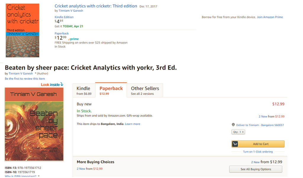
If you are passionate about cricket, and love analyzing cricket performances, then check out my 2 racy books on cricket! In my books, I perform detailed yet compact analysis of performances of both batsmen, bowlers besides evaluating team & match performances in Tests , ODIs, T20s & IPL. You can buy my books on cricket from Amazon at $12.99 for the paperback and $4.99/$6.99 respectively for the kindle versions. The books can be accessed at Cricket analytics with cricketr and Beaten by sheer pace-Cricket analytics with yorkr A must read for any cricket lover! Check it out!!

Feel free to download/clone these templates from Github yorkrT20Template and perform your own analysis

There will be 5 folders at the root

T20data – Match files as yaml from Cricsheet
T20Matches – Yaml match files converted to dataframes
T20MatchesBetween2Teams – All Matches between any 2 T20 teams
allMatchesAllOpposition – A T20 countries match data against all other teams
BattingBowlingDetails – Batting and bowling details of all countries

library(yorkr)
library(dplyr)

The first few steps take care of the data setup. This needs to be done before any of the analysis of T20 batsmen, bowlers, any T20 match, matches between any 2 T20 countries or analysis of a teams performance against all other countries

There will be 5 folders at the root

T20data
T20Matches
T20MatchesBetween2Teams
allMatchesAllOpposition
BattingBowlingDetails

The source YAML files will be in T20Data folder

1.Create directory T20Matches

Some files may give conversions errors. You could try to debug the problem or just remove it from the T20data folder. At most 2-4 file will have conversion problems and I usally remove then from the files to be converted.

Also take a look at my Inswinger shiny app which was created after performing the same conversion on the Dec 16 data .

convertAllYaml2RDataframesT20("T20Data","T20Matches")

2.Save all matches between all combinations of T20 nations

This function will create the set of all matches between every T20 country against every other T20 country. This uses the data that was created in T20Matches, with the convertAllYaml2RDataframesT20() function.

setwd("./T20MatchesBetween2Teams")
saveAllMatchesBetweenTeams(dir=".",odir=".")

3.Save all matches against all opposition

This will create a consolidated dataframe of all matches played by every T20 playing nation against all other nattions. This also uses the data that was created in T20Matches, with the convertAllYaml2RDataframesT20() function.

setwd("../allMatchesAllOpposition")
saveAllMatchesAllOpposition(dir=".",odir=".")

4. Create batting and bowling details for each T20 country

These are the current T20 playing nations. You can add to this vector as more countries start playing T20. You will get to know all T20 nations by also look at the directory created above namely allMatchesAllOpposition. his also uses the data that was created in T20Matches, with the convertAllYaml2RDataframesT20() function.

setwd("../BattingBowlingDetails")
teams <-c("Australia","India","Pakistan","West Indies", 'Sri Lanka',
          "England", "Bangladesh","Netherlands","Scotland", "Afghanistan",
          "Zimbabwe","Ireland","New Zealand","South Africa","Canada",
          "Bermuda","Kenya","Hong Kong","Nepal","Oman","Papua New Guinea",
          "United Arab Emirates")

for(i in seq_along(teams)){
    print(teams[i])
    val <- paste(teams[i],"-details",sep="")
    val <- getTeamBattingDetails(teams[i],dir="../T20Matches", save=TRUE)

}

for(i in seq_along(teams)){
    print(teams[i])
    val <- paste(teams[i],"-details",sep="")
    val <- getTeamBowlingDetails(teams[i],dir="../T20Matches", save=TRUE)

}

5. Get the list of batsmen for a particular country

For e.g. if you wanted to get the batsmen of Canada you would do the following. By replacing Canada for any other country you can get the batsmen of that country. These batsmen names can then be used in the batsmen analysis

country="Canada"
teamData <- paste(country,"-BattingDetails.RData",sep="")
load(teamData)
countryDF <- battingDetails
bmen <- countryDF %>% distinct(batsman) 
bmen <- as.character(bmen$batsman)
batsmen <- sort(bmen)
batsmen

6. Get the list of bowlers for a particular country

The method below can get the list of bowler names for any T20 nation. These names can then be used in the bowler analysis below

country="Netherlands"
teamData <- paste(country,"-BowlingDetails.RData",sep="")
load(teamData)
countryDF <- bowlingDetails
bwlr <- countryDF %>% distinct(bowler) 
bwlr <- as.character(bwlr$bowler)
bowler <- sort(bwlr)
bowler

Now we are all set

A) International T20 Match Analysis

Load any match data from the ./T20Matches folder for e.g. Afganistan-England-2016-03-23.RData

setwd("./T20Matches")
load("Afghanistan-England-2016-03-23.RData")
afg_eng<- overs
#The steps are
load("Country1-Country2-Date.Rdata")
country1_country2 <- overs

All analysis for this match can be done now

2. Scorecard

teamBattingScorecardMatch(country1_country2,"Country1")
teamBattingScorecardMatch(country1_country2,"Country2")

3.Batting Partnerships

teamBatsmenPartnershipMatch(country1_country2,"Country1","Country2")
teamBatsmenPartnershipMatch(country1_country2,"Country2","Country1")

4. Batsmen vs Bowler Plot

teamBatsmenVsBowlersMatch(country1_country2,"Country1","Country2",plot=TRUE)
teamBatsmenVsBowlersMatch(country1_country2,"Country1","Country2",plot=FALSE)

5. Team bowling scorecard

teamBowlingScorecardMatch(country1_country2,"Country1")
teamBowlingScorecardMatch(country1_country2,"Country2")

6. Team bowling Wicket kind match

teamBowlingWicketKindMatch(country1_country2,"Country1","Country2")
m <-teamBowlingWicketKindMatch(country1_country2,"Country1","Country2",plot=FALSE)
m

7. Team Bowling Wicket Runs Match

teamBowlingWicketRunsMatch(country1_country2,"Country1","Country2")
m <-teamBowlingWicketRunsMatch(country1_country2,"Country1","Country2",plot=FALSE)
m

8. Team Bowling Wicket Match

m <-teamBowlingWicketMatch(country1_country2,"Country1","Country2",plot=FALSE)
m
teamBowlingWicketMatch(country1_country2,"Country1","Country2")

9. Team Bowler vs Batsmen

teamBowlersVsBatsmenMatch(country1_country2,"Country1","Country2")
m <- teamBowlersVsBatsmenMatch(country1_country2,"Country1","Country2",plot=FALSE)
m

10. Match Worm chart

matchWormGraph(country1_country2,"Country1","Country2")

B) International T20 Matches between 2 teams

Load match data between any 2 teams from ./T20MatchesBetween2Teams for e.g.Australia-India-allMatches

setwd("./T20MatchesBetween2Teams")
load("Australia-India-allMatches.RData")
aus_ind_matches <- matches
#Replace below with your own countries
country1<-"England"
country2 <- "South Africa"
country1VsCountry2 <- paste(country1,"-",country2,"-allMatches.RData",sep="")
load(country1VsCountry2)
country1_country2_matches <- matches

2.Batsmen partnerships

m<- teamBatsmenPartnershiOppnAllMatches(country1_country2_matches,"country1",report="summary")
m
m<- teamBatsmenPartnershiOppnAllMatches(country1_country2_matches,"country2",report="summary")
m
m<- teamBatsmenPartnershiOppnAllMatches(country1_country2_matches,"country1",report="detailed")
m
teamBatsmenPartnershipOppnAllMatchesChart(country1_country2_matches,"country1","country2")

3. Team batsmen vs bowlers

teamBatsmenVsBowlersOppnAllMatches(country1_country2_matches,"country1","country2")

4. Bowling scorecard

a <-teamBattingScorecardOppnAllMatches(country1_country2_matches,main="country1",opposition="country2")
a

5. Team bowling performance

teamBowlingPerfOppnAllMatches(country1_country2_matches,main="country1",opposition="country2")

6. Team bowler wickets

teamBowlersWicketsOppnAllMatches(country1_country2_matches,main="country1",opposition="country2")
m <-teamBowlersWicketsOppnAllMatches(country1_country2_matches,main="country1",opposition="country2",plot=FALSE)
teamBowlersWicketsOppnAllMatches(country1_country2_matches,"country1","country2",top=3)
m

7. Team bowler vs batsmen

teamBowlersVsBatsmenOppnAllMatches(country1_country2_matches,"country1","country2",top=5)

8. Team bowler wicket kind

teamBowlersWicketKindOppnAllMatches(country1_country2_matches,"country1","country2",plot=TRUE)
m <- teamBowlersWicketKindOppnAllMatches(country1_country2_matches,"country1","country2",plot=FALSE)
m[1:30,]

9. Team bowler wicket runs

teamBowlersWicketRunsOppnAllMatches(country1_country2_matches,"country1","country2")

10. Plot wins and losses

setwd("./T20Matches")
plotWinLossBetweenTeams("country1","country2")

C) International T20 Matches for a team against all other teams

Load the data between for a T20 team against all other countries ./allMatchesAllOpposition for e.g all matches of India

load("allMatchesAllOpposition-India.RData")
india_matches <- matches
country="country1"
allMatches <- paste("allMatchesAllOposition-",country,".RData",sep="")
load(allMatches)
country1AllMatches <- matches

2. Team’s batting scorecard all Matches

m <-teamBattingScorecardAllOppnAllMatches(country1AllMatches,theTeam="country1")
m

3. Batting scorecard of opposing team

m <-teamBattingScorecardAllOppnAllMatches(matches=country1AllMatches,theTeam="country2")

4. Team batting partnerships

m <- teamBatsmenPartnershipAllOppnAllMatches(country1AllMatches,theTeam="country1")
m
m <- teamBatsmenPartnershipAllOppnAllMatches(country1AllMatches,theTeam='country1',report="detailed")
head(m,30)
m <- teamBatsmenPartnershipAllOppnAllMatches(country1AllMatches,theTeam='country1',report="summary")
m

5. Team batting partnerships plot

teamBatsmenPartnershipAllOppnAllMatchesPlot(country1AllMatches,"country1",main="country1")
teamBatsmenPartnershipAllOppnAllMatchesPlot(country1AllMatches,"country1",main="country2")

6, Team batsmen vs bowlers report

m <-teamBatsmenVsBowlersAllOppnAllMatchesRept(country1AllMatches,"country1",rank=0)
m
m <-teamBatsmenVsBowlersAllOppnAllMatchesRept(country1AllMatches,"country1",rank=1,dispRows=30)
m
m <-teamBatsmenVsBowlersAllOppnAllMatchesRept(matches=country1AllMatches,theTeam="country2",rank=1,dispRows=25)
m

7. Team batsmen vs bowler plot

d <- teamBatsmenVsBowlersAllOppnAllMatchesRept(country1AllMatches,"country1",rank=1,dispRows=50)
d
teamBatsmenVsBowlersAllOppnAllMatchesPlot(d)
d <- teamBatsmenVsBowlersAllOppnAllMatchesRept(country1AllMatches,"country1",rank=2,dispRows=50)
teamBatsmenVsBowlersAllOppnAllMatchesPlot(d)

8. Team bowling scorecard

teamBowlingScorecardAllOppnAllMatchesMain(matches=country1AllMatches,theTeam="country1")
teamBowlingScorecardAllOppnAllMatches(country1AllMatches,'country2')

9. Team bowler vs batsmen

teamBowlersVsBatsmenAllOppnAllMatchesMain(country1AllMatches,theTeam="country1",rank=0)
teamBowlersVsBatsmenAllOppnAllMatchesMain(country1AllMatches,theTeam="country1",rank=2)
teamBowlersVsBatsmenAllOppnAllMatchesRept(matches=country1AllMatches,theTeam="country1",rank=0)

10. Team Bowler vs bastmen

df <- teamBowlersVsBatsmenAllOppnAllMatchesRept(country1AllMatches,theTeam="country1",rank=1)
teamBowlersVsBatsmenAllOppnAllMatchesPlot(df,"country1","country1")

11. Team bowler wicket kind

teamBowlingWicketKindAllOppnAllMatches(country1AllMatches,t1="country1",t2="All")
teamBowlingWicketKindAllOppnAllMatches(country1AllMatches,t1="country1",t2="country2")

12.

teamBowlingWicketRunsAllOppnAllMatches(country1AllMatches,t1="country1",t2="All",plot=TRUE)
teamBowlingWicketRunsAllOppnAllMatches(country1AllMatches,t1="country1",t2="country2",plot=TRUE)

D) Batsman functions

Get the batsman’s details for a batsman

setwd("../BattingBowlingDetails")
kohli <- getBatsmanDetails(team="India",name="Kohli",dir=".")
batsmanDF <- getBatsmanDetails(team="country1",name="batsmanName",dir=".")

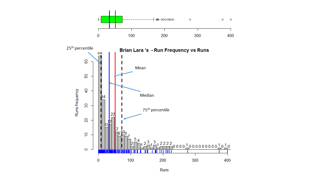
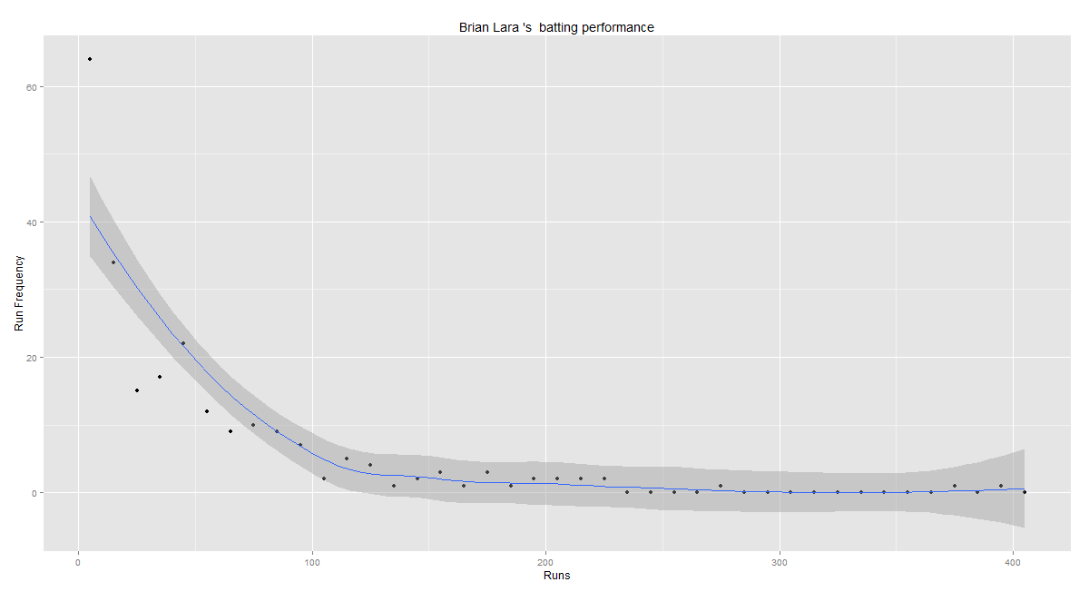
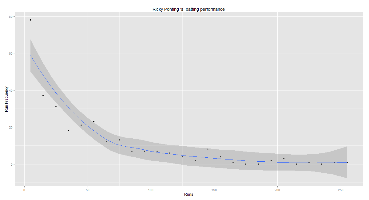
2. Runs vs deliveries

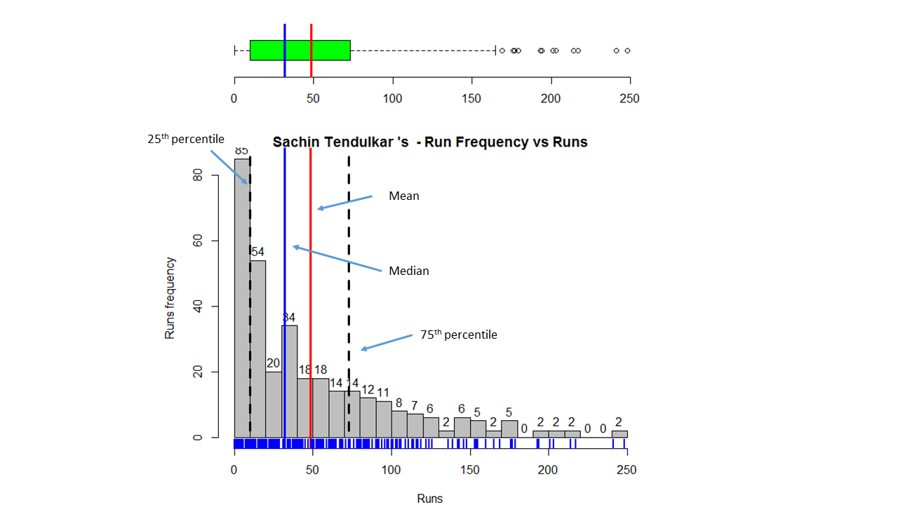
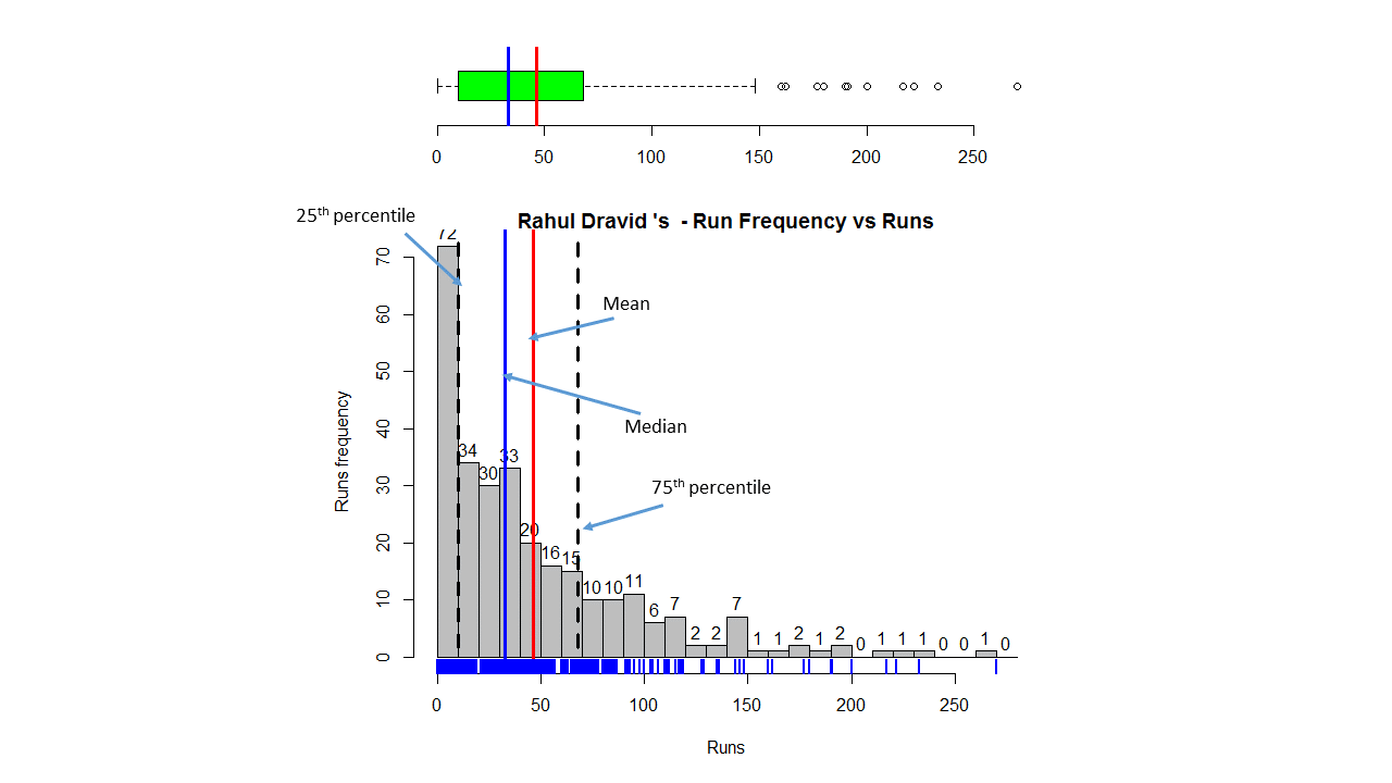
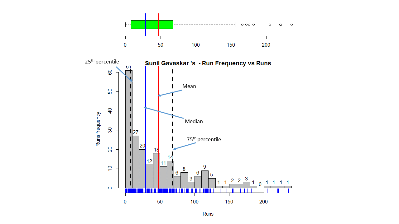
batsmanRunsVsDeliveries(batsmanDF,"batsmanName")

3. Batsman 4s & 6s

batsman46 <- select(batsmanDF,batsman,ballsPlayed,fours,sixes,runs)
p1 <- batsmanFoursSixes(batsman46,"batsmanName")

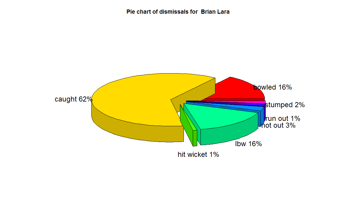
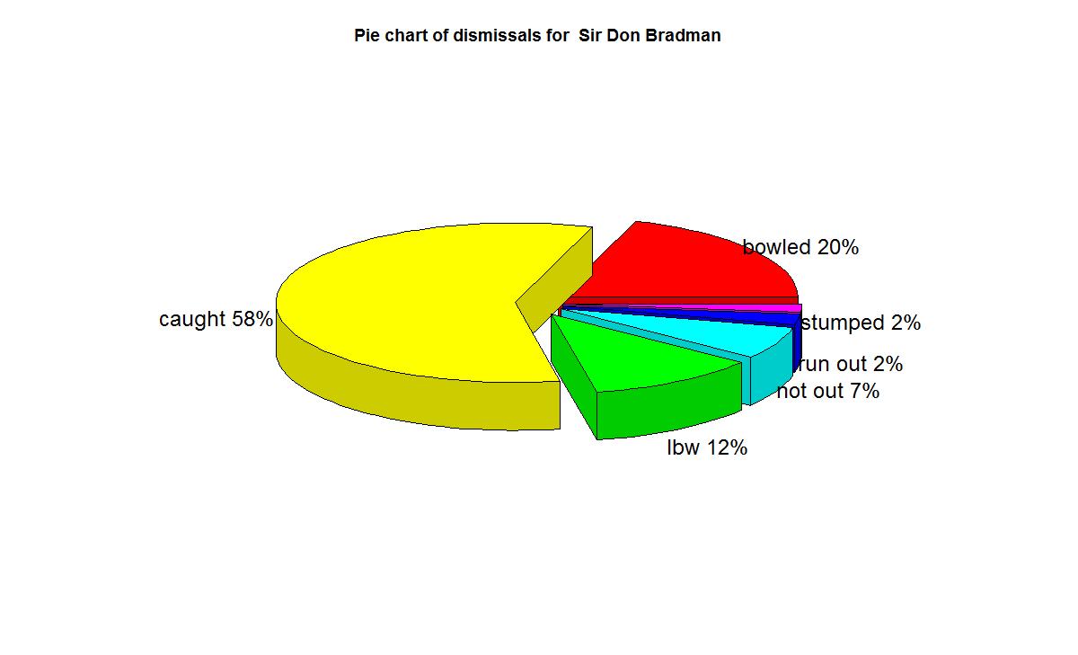
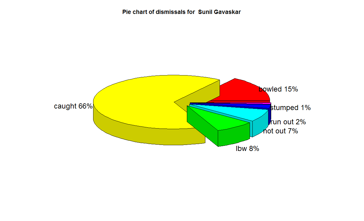
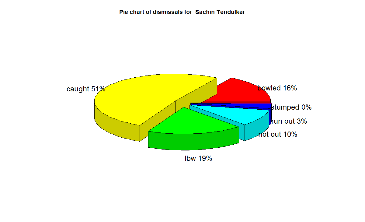
4. Batsman dismissals

batsmanDismissals(batsmanDF,"batsmanName")

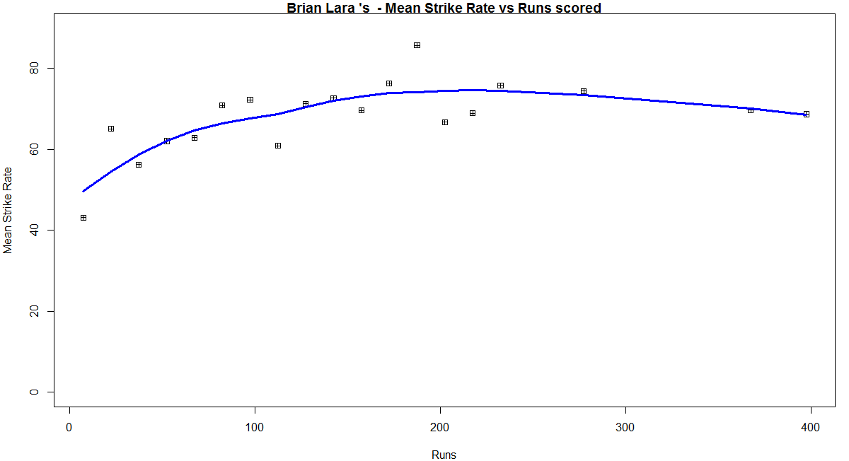
5. Runs vs Strike rate

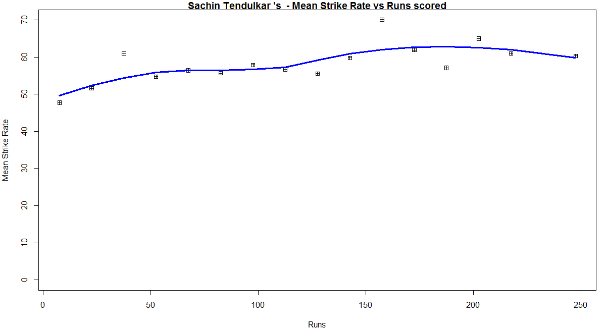
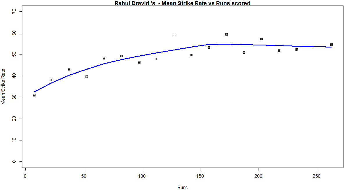
batsmanRunsVsStrikeRate(batsmanDF,"batsmanName")

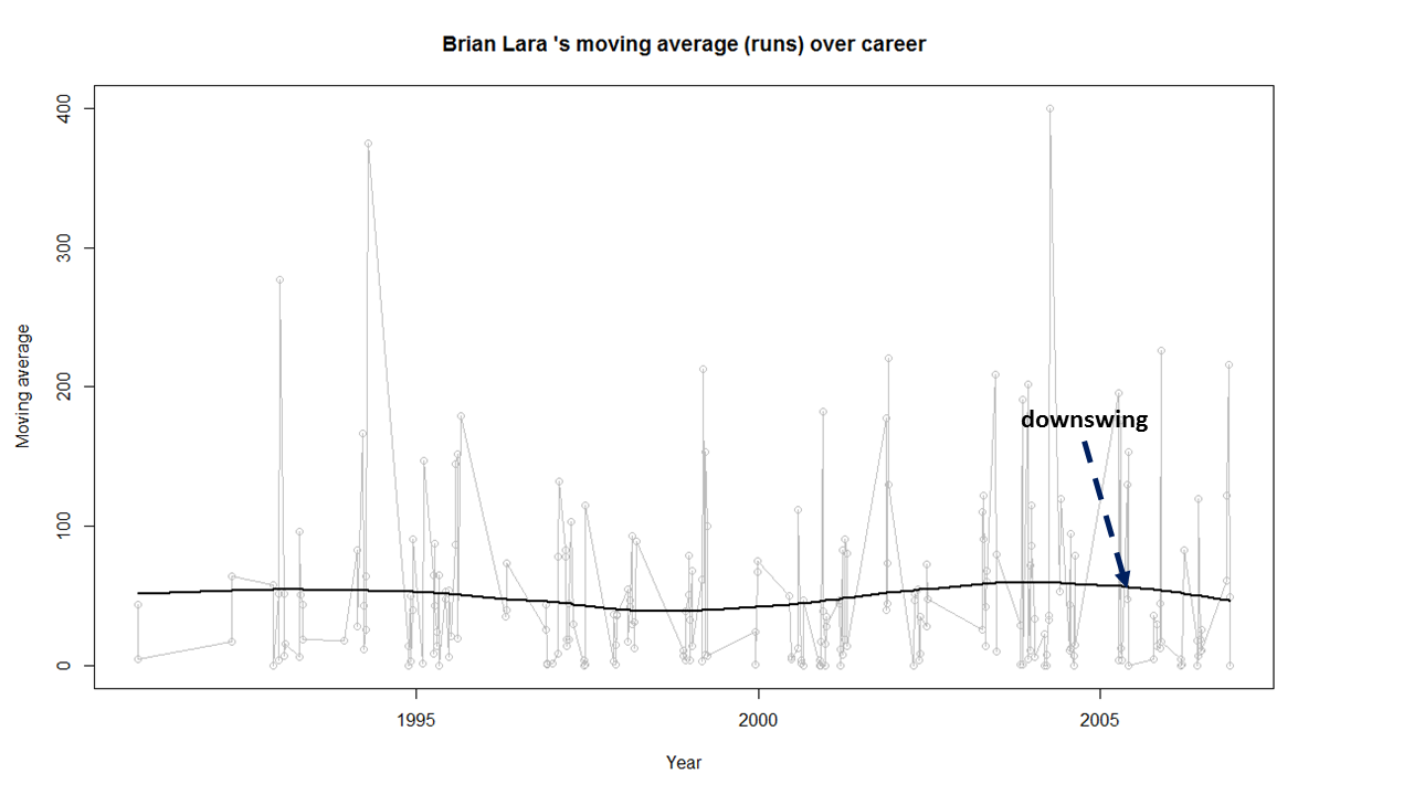
6. Batsman Moving Average

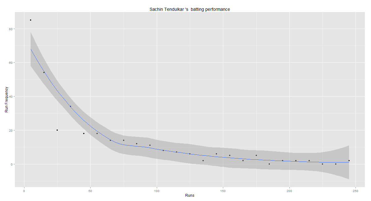
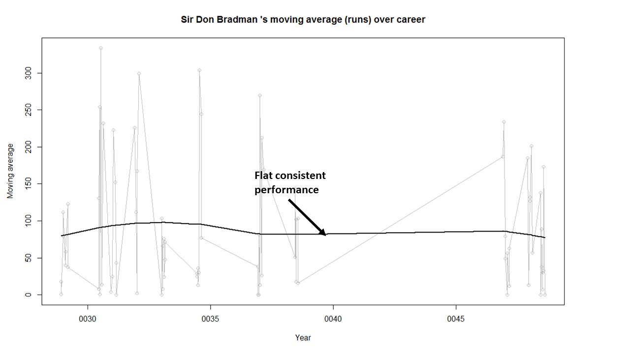
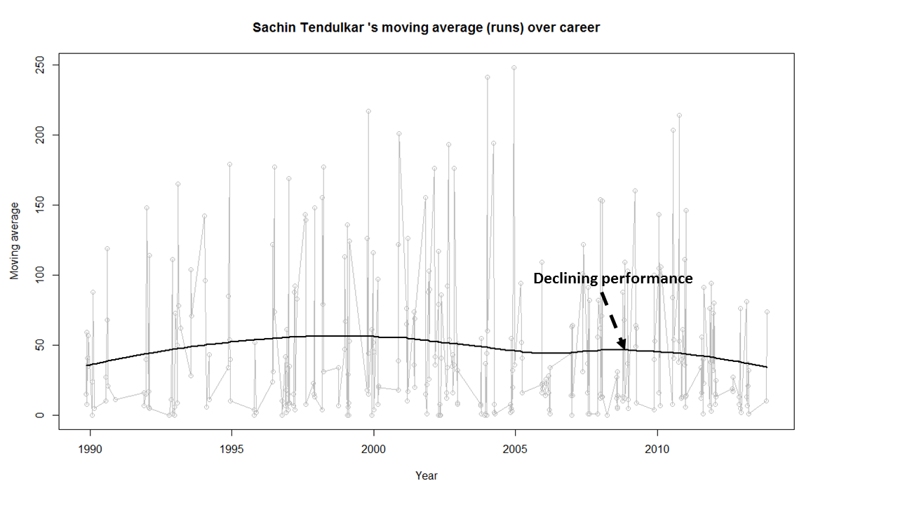
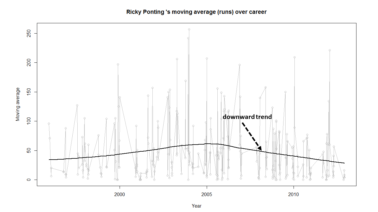
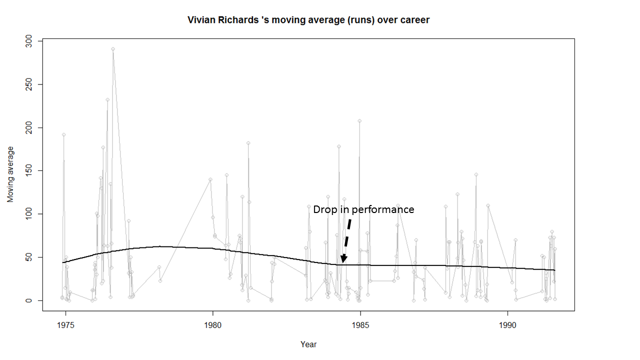
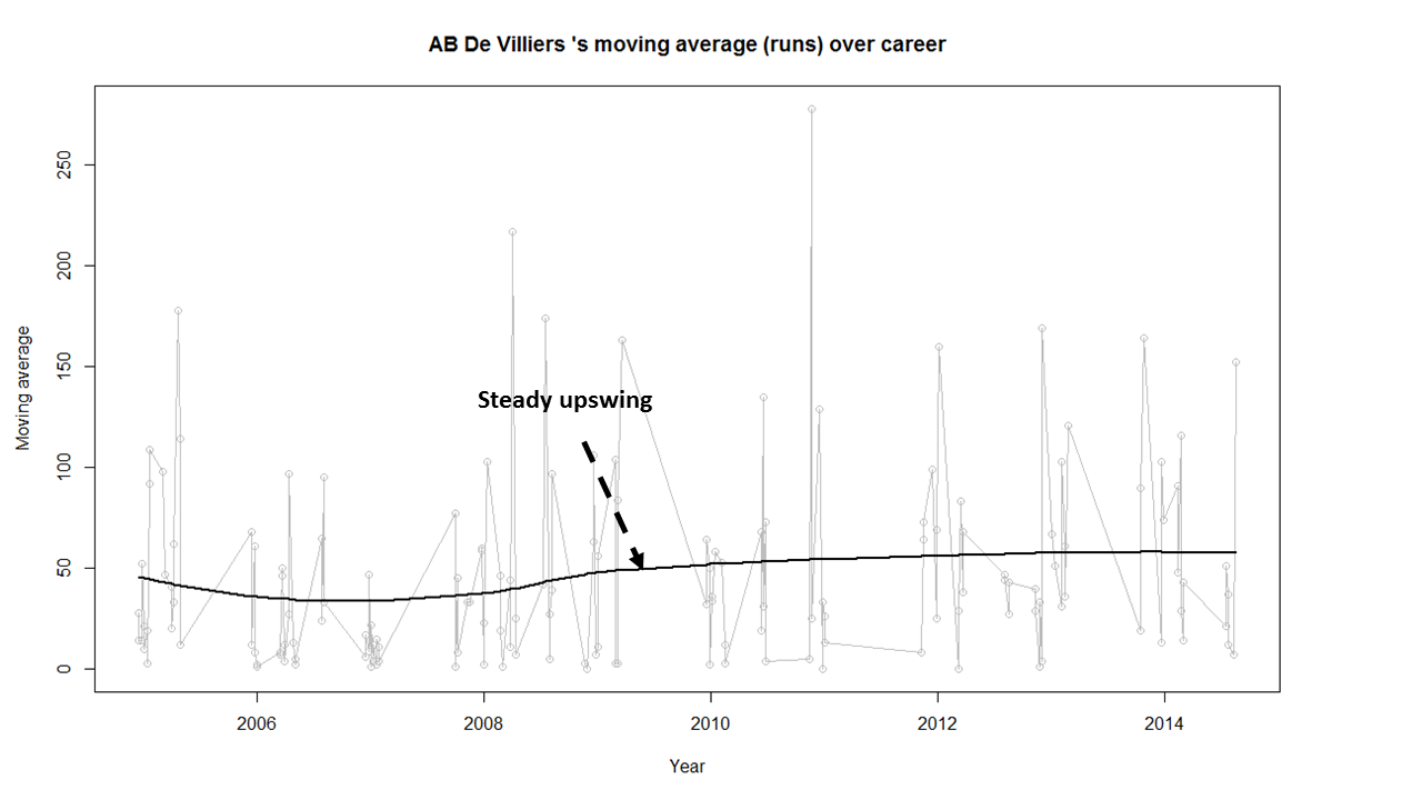
batsmanMovingAverage(batsmanDF,"batsmanName")

7. Batsman cumulative average

batsmanCumulativeAverageRuns(batsmanDF,"batsmanName")

8. Batsman cumulative strike rate

batsmanCumulativeStrikeRate(batsmanDF,"batsmanName")

9. Batsman runs against oppositions

batsmanRunsAgainstOpposition(batsmanDF,"batsmanName")

10. Batsman runs vs venue

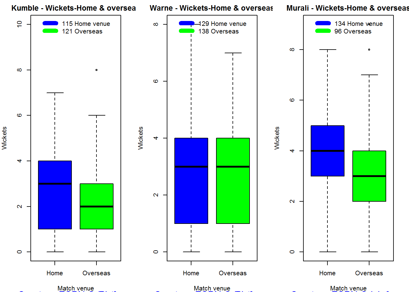
batsmanRunsVenue(batsmanDF,"batsmanName")

11. Batsman runs predict

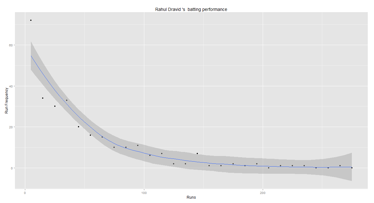
batsmanRunsPredict(batsmanDF,"batsmanName")

12. Bowler functions

For example to get Ravicahnder Ashwin’s bowling details

setwd("../BattingBowlingDetails")
ashwin <- getBowlerWicketDetails(team="India",name="Ashwin",dir=".")
bowlerDF <- getBatsmanDetails(team="country1",name="bowlerName",dir=".")

13. Bowler Mean Economy rate

bowlerMeanEconomyRate(bowlerDF,"bowlerName")

14. Bowler mean runs conceded

bowlerMeanRunsConceded(bowlerDF,"bowlerName")

15. Bowler Moving Average

bowlerMovingAverage(bowlerDF,"bowlerName")

16. Bowler cumulative average wickets

bowlerCumulativeAvgWickets(bowlerDF,"bowlerName")

17. Bowler cumulative Economy Rate (ER)

bowlerCumulativeAvgEconRate(bowlerDF,"bowlerName")

18. Bowler wicket plot

bowlerWicketPlot(bowlerDF,"bowlerName")

19. Bowler wicket against opposition

bowlerWicketsAgainstOpposition(bowlerDF,"bowlerName")

20. Bowler wicket at cricket grounds

bowlerWicketsVenue(bowlerDF,"bowlerName")

21. Predict number of deliveries to wickets

setwd("./T20Matches")
bowlerDF1 <- getDeliveryWickets(team="country1",dir=".",name="bowlerName",save=FALSE)
bowlerWktsPredict(bowlerDF1,"bowlerName")

Revisiting crimes against women in India

Here I go again, raking the muck about crimes against women in India. My earlier post “A crime map of India in R: Crimes against women in India” garnered a lot of responses from readers. In fact one of the readers even volunteered to create the only choropleth map in that post. The data for this post is taken from http://data.gov.in. You can download the data from the link “Crimes against women in India”

I was so impressed by the choropleth map that I decided to do that for all crimes against women.(Wikipedia definition: A choropleth map is a thematic map in which areas are shaded or patterned in proportion to the measurement of the statistical variable being displayed on the map). Personally, I think pictures tell the story better. I am sure you will agree!

So here, I have it a Shiny app which will plot choropleth maps for a chosen crime in a given year.

You can try out my interactive Shiny app at Crimes against women in India

Checkout out my book on Amazon available in both Paperback ($9.99) and a Kindle version($6.99/Rs449/). (see ‘Practical Machine Learning with R and Python – Machine Learning in stereo‘)

The following technique can be used to determine the ‘goodness’ of a hypothesis or how well the hypothesis can fit the data and can also generalize to new examples not in the training set.

In the picture below are the details of ‘Rape” in the year 2015.

Interestingly the ‘Total Crime against women’ in 2001 shows the Top 5 as
1) Uttar Pradresh 2) Andhra Pradesh 3) Madhya Pradesh 4) Maharashtra 5) Rajasthan

But in 2015 West Bengal tops the list, as the real heavy weight in crimes against women. The new pecking order in 2015 for ‘Total Crimes against Women’ is

1) West Bengal 2) Andhra Pradesh 3) Uttar Pradesh 4) Rajasthan 5) Maharashtra

Similarly for rapes, West Bengal is nowhere in the top 5 list in 2001. In 2015, it is in second only to the national rape leader Madhya Pradesh. Also in 2001 West Bengal is not in the top 5 for any of 6 crime heads. But in 2015, West Bengal is in the top 5 of 6 crime heads. The emergence of West Bengal as the leader in Crimes against Women is due to the steep increase in crime rate over the years.Clearly the law and order situation in West Bengal is heading south.

In Dowry Deaths, UP, Bihar, MP, West Bengal lead the pack, and in that order in 2015.

The usual suspects for most crime categories are West Bengal, UP, MP, AP & Maharashtra.

The state-wise crime charts plot the incidence of the crime (rape, dowry death, assault on women etc) over the years. Data for each state and for each crime was available from 2001-2013. The data for period 2014-2018 are projected using linear regression. The shaded portion in the plots indicate the 95% confidence level in the prediction (i.e in other words we can be 95% certain that the true mean of the crime rate in the projected years will lie within the shaded region)

Several interesting requests came from readers to my earlier post. Some of them were to to plot the crimes as function of population and per capita income of the State/Union Territory to see if the plots throw up new crime leaders. I have not got the relevant state-wise population distribution data yet. I intend to update this when I get my hands on this data.

I have included the crimes.csv which has been used to generate the visualization. However for the Shiny app I save this as .RData for better performance of the app.

You can clone/download the code for the Shiny app from GitHub at crimesAgainWomenIndia

Please checkout my Shiny app : Crimes against women

I also intend to add further interactivity to my visualizations in a future version. Watch this space. I’ll be back!

Introducing cricketr! : An R package to analyze performances of cricketers

Yet all experience is an arch wherethro’
Gleams that untravell’d world whose margin fades
For ever and forever when I move.
How dull it is to pause, to make an end,
To rust unburnish’d, not to shine in use!
Ulysses by Alfred Tennyson

Introduction

This is an initial post in which I introduce a cricketing package ‘cricketr’ which I have created. This package was a natural culmination to my earlier posts on cricket and my finishing 10 modules of Data Science Specialization, from John Hopkins University at Coursera. The thought of creating this package struck me some time back, and I have finally been able to bring this to fruition.

So here it is. My R package ‘cricketr!!!’

You can download the latest PDF version of the book at ‘Cricket analytics with cricketr and cricpy: Analytics harmony with R and Python-6th edition‘

Untitled

This package uses the statistics info available in ESPN Cricinfo Statsguru. The current version of this package can handle all formats of the game including Test, ODI and Twenty20 cricket.

You should be able to install the package from CRAN and use many of the functions available in the package. Please be mindful of ESPN Cricinfo Terms of Use

(Note: This page is also hosted as a GitHub page at cricketr and also at RPubs as cricketr: A R package for analyzing performances of cricketers

You can download this analysis as a PDF file from Introducing cricketr

Note: If you would like to do a similar analysis for a different set of batsman and bowlers, you can clone/download my skeleton cricketr template from Github (which is the R Markdown file I have used for the analysis below). You will only need to make appropriate changes for the players you are interested in. Just a familiarity with R and R Markdown only is needed.

You can clone the cricketr code from Github at cricketr

(Take a look at my short video tutorial on my R package cricketr on Youtube – R package cricketr – A short tutorial)

Do check out my interactive Shiny app implementation using the cricketr package – Sixer – R package cricketr’s new Shiny avatar

Please look at my recent post, which includes updates to this post, and 8 new functions added to the cricketr package “Re-introducing cricketr: An R package to analyze the performances of cricketers”

Important note 1: The latest release of ‘cricketr’ now includes the ability to analyze performances of teams now!! See Cricketr adds team analytics to its repertoire!!!

Important note 2 : Cricketr can now do a more fine-grained analysis of players, see Cricketr learns new tricks : Performs fine-grained analysis of players

Important note 3: Do check out the python avatar of cricketr, ‘cricpy’ in my post ‘Introducing cricpy:A python package to analyze performances of cricketers”

The cricketr package

The cricketr package has several functions that perform several different analyses on both batsman and bowlers. The package has functions that plot percentage frequency runs or wickets, runs likelihood for a batsman, relative run/strike rates of batsman and relative performance/economy rate for bowlers are available.

Other interesting functions include batting performance moving average, forecast and a function to check whether the batsman/bowler is in in-form or out-of-form.

The data for a particular player can be obtained with the getPlayerData() function from the package. To do this you will need to go to ESPN CricInfo Player and type in the name of the player for e.g Ricky Ponting, Sachin Tendulkar etc. This will bring up a page which have the profile number for the player e.g. for Sachin Tendulkar this would be http://www.espncricinfo.com/india/content/player/35320.html. Hence, Sachin’s profile is 35320. This can be used to get the data for Tendulkar as shown below

The cricketr package is now available from CRAN!!!. You should be able to install directly with

if (!require("cricketr")){ 
    install.packages("cricketr",lib = "c:/test") 
} 
library(cricketr)

?getPlayerData

## 
## getPlayerData(profile, opposition='', host='', dir='./data', file='player001.csv', type='batting', homeOrAway=[1, 2], result=[1, 2, 4], create=True)
##     Get the player data from ESPN Cricinfo based on specific inputs and store in a file in a given directory
##     
##     Description
##     
##     Get the player data given the profile of the batsman. The allowed inputs are home,away or both and won,lost or draw of matches. The data is stored in a .csv file in a directory specified. This function also returns a data frame of the player
##     
##     Usage
##     
##     getPlayerData(profile,opposition="",host="",dir="./data",file="player001.csv",
##     type="batting", homeOrAway=c(1,2),result=c(1,2,4))
##     Arguments
##     
##     profile     
##     This is the profile number of the player to get data. This can be obtained from http://www.espncricinfo.com/ci/content/player/index.html. Type the name of the player and click search. This will display the details of the player. Make a note of the profile ID. For e.g For Sachin Tendulkar this turns out to be http://www.espncricinfo.com/india/content/player/35320.html. Hence the profile for Sachin is 35320
##     opposition  
##     The numerical value of the opposition country e.g.Australia,India, England etc. The values are Australia:2,Bangladesh:25,England:1,India:6,New Zealand:5,Pakistan:7,South Africa:3,Sri Lanka:8, West Indies:4, Zimbabwe:9
##     host        
##     The numerical value of the host country e.g.Australia,India, England etc. The values are Australia:2,Bangladesh:25,England:1,India:6,New Zealand:5,Pakistan:7,South Africa:3,Sri Lanka:8, West Indies:4, Zimbabwe:9
##     dir 
##     Name of the directory to store the player data into. If not specified the data is stored in a default directory "./data". Default="./data"
##     file        
##     Name of the file to store the data into for e.g. tendulkar.csv. This can be used for subsequent functions. Default="player001.csv"
##     type        
##     type of data required. This can be "batting" or "bowling"
##     homeOrAway  
##     This is a vector with either 1,2 or both. 1 is for home 2 is for away
##     result      
##     This is a vector that can take values 1,2,4. 1 - won match 2- lost match 4- draw
##     Details
##     
##     More details can be found in my short video tutorial in Youtube https://www.youtube.com/watch?v=q9uMPFVsXsI
##     
##     Value
##     
##     Returns the player's dataframe
##     
##     Note
##     
##     Maintainer: Tinniam V Ganesh <tvganesh.85@gmail.com>
##     
##     Author(s)
##     
##     Tinniam V Ganesh
##     
##     References
##     
##     http://www.espncricinfo.com/ci/content/stats/index.html
##     https://gigadom.wordpress.com/
##     
##     See Also
##     
##     getPlayerDataSp
##     
##     Examples
##     
##     ## Not run: 
##     # Both home and away. Result = won,lost and drawn
##     tendulkar = getPlayerData(35320,dir=".", file="tendulkar1.csv",
##     type="batting", homeOrAway=c(1,2),result=c(1,2,4))
##     
##     # Only away. Get data only for won and lost innings
##     tendulkar = getPlayerData(35320,dir=".", file="tendulkar2.csv",
##     type="batting",homeOrAway=c(2),result=c(1,2))
##     
##     # Get bowling data and store in file for future
##     kumble = getPlayerData(30176,dir=".",file="kumble1.csv",
##     type="bowling",homeOrAway=c(1),result=c(1,2))
##     
##     #Get the Tendulkar's Performance against Australia in Australia
##     tendulkar = getPlayerData(35320, opposition = 2,host=2,dir=".", 
##     file="tendulkarVsAusInAus.csv",type="batting")

The cricketr package includes some pre-packaged sample (.csv) files. You can use these sample to test functions as shown below

# Retrieve the file path of a data file installed with cricketr
pathToFile ,"Sachin Tendulkar")

Alternatively, the cricketr package can be installed from GitHub with

if (!require("cricketr")){ 
    library(devtools) 
    install_github("tvganesh/cricketr") 
}
library(cricketr)

The pre-packaged files can be accessed as shown above.
To get the data of any player use the function getPlayerData()

tendulkar <- getPlayerData(35320,dir="..",file="tendulkar.csv",type="batting",homeOrAway=c(1,2),
                           result=c(1,2,4))

Important Note This needs to be done only once for a player. This function stores the player’s data in a CSV file (for e.g. tendulkar.csv as above) which can then be reused for all other functions. Once we have the data for the players many analyses can be done. This post will use the stored CSV file obtained with a prior getPlayerData for all subsequent analyses

Sachin Tendulkar’s performance – Basic Analyses

The 3 plots below provide the following for Tendulkar

Frequency percentage of runs in each run range over the whole career
Mean Strike Rate for runs scored in the given range
A histogram of runs frequency percentages in runs ranges

par(mfrow=c(1,3))
par(mar=c(4,4,2,2))
batsmanRunsFreqPerf("./tendulkar.csv","Sachin Tendulkar")
batsmanMeanStrikeRate("./tendulkar.csv","Sachin Tendulkar")
batsmanRunsRanges("./tendulkar.csv","Sachin Tendulkar")

dev.off()

## null device 
##           1

More analyses

par(mfrow=c(1,3))
par(mar=c(4,4,2,2))
batsman4s("./tendulkar.csv","Tendulkar")
batsman6s("./tendulkar.csv","Tendulkar")
batsmanDismissals("./tendulkar.csv","Tendulkar")

3D scatter plot and prediction plane

The plots below show the 3D scatter plot of Sachin’s Runs versus Balls Faced and Minutes at crease. A linear regression model is then fitted between Runs and Balls Faced + Minutes at crease

battingPerf3d("./tendulkar.csv","Sachin Tendulkar")

Average runs at different venues

The plot below gives the average runs scored by Tendulkar at different grounds. The plot also displays the number of innings at each ground as a label at x-axis. It can be seen Tendulkar did great in Colombo (SSC), Melbourne ifor matches overseas and Mumbai, Mohali and Bangalore at home

batsmanAvgRunsGround("./tendulkar.csv","Sachin Tendulkar")

Average runs against different opposing teams

This plot computes the average runs scored by Tendulkar against different countries. The x-axis also gives the number of innings against each team

batsmanAvgRunsOpposition("./tendulkar.csv","Tendulkar")

Highest Runs Likelihood

The plot below shows the Runs Likelihood for a batsman. For this the performance of Sachin is plotted as a 3D scatter plot with Runs versus Balls Faced + Minutes at crease using. K-Means. The centroids of 3 clusters are computed and plotted. In this plot. Sachin Tendulkar’s highest tendencies are computed and plotted using K-Means

batsmanRunsLikelihood("./tendulkar.csv","Sachin Tendulkar")

## Summary of  Sachin Tendulkar 's runs scoring likelihood
## **************************************************
## 
## There is a 16.51 % likelihood that Sachin Tendulkar  will make  139 Runs in  251 balls over 353  Minutes 
## There is a 58.41 % likelihood that Sachin Tendulkar  will make  16 Runs in  31 balls over  44  Minutes 
## There is a 25.08 % likelihood that Sachin Tendulkar  will make  66 Runs in  122 balls over 167  Minutes

A look at the Top 4 batsman – Tendulkar, Kallis, Ponting and Sangakkara

The batsmen with the most hundreds in test cricket are

Sachin Tendulkar :Average:53.78,100’s – 51, 50’s – 68
Jacques Kallis : Average: 55.47, 100’s – 45, 50’s – 58
Ricky Ponting : Average: 51.85, 100’s – 41 , 50’s – 62
Kumara Sangakarra: Average: 58.04 ,100’s – 38 , 50’s – 52

in that order.

The following plots take a closer at their performances. The box plots show the mean (red line) and median (blue line). The two ends of the boxplot display the 25th and 75th percentile.

Box Histogram Plot

This plot shows a combined boxplot of the Runs ranges and a histogram of the Runs Frequency. The calculated Mean differ from the stated means possibly because of data cleaning. Also not sure how the means were arrived at ESPN Cricinfo for e.g. when considering not out..

batsmanPerfBoxHist("./tendulkar.csv","Sachin Tendulkar")

batsmanPerfBoxHist("./kallis.csv","Jacques Kallis")

batsmanPerfBoxHist("./ponting.csv","Ricky Ponting")

batsmanPerfBoxHist("./sangakkara.csv","K Sangakkara")

Contribution to won and lost matches

The plot below shows the contribution of Tendulkar, Kallis, Ponting and Sangakarra in matches won and lost. The plots show the range of runs scored as a boxplot (25th & 75th percentile) and the mean scored. The total matches won and lost are also printed in the plot.

All the players have scored more in the matches they won than the matches they lost. Ricky Ponting is the only batsman who seems to have more matches won to his credit than others. This could also be because he was a member of strong Australian team

For the next 2 functions below you will have to use the getPlayerDataSp() function. I
have commented this as I already have these files

tendulkarsp

par(mfrow=c(2,2))
par(mar=c(4,4,2,2))
batsmanContributionWonLost("tendulkarsp.csv","Tendulkar")
batsmanContributionWonLost("kallissp.csv","Kallis")
batsmanContributionWonLost("pontingsp.csv","Ponting")
batsmanContributionWonLost("sangakkarasp.csv","Sangakarra")

dev.off()

## null device 
##           1

Performance at home and overseas

From the plot below it can be seen
Tendulkar has more matches overseas than at home and his performance is consistent in all venues at home or abroad. Ponting has lesser innings than Tendulkar and has an equally good performance at home and overseas.Kallis and Sangakkara’s performance abroad is lower than the performance at home.

This function also requires the use of getPlayerDataSp() as shown above

par(mfrow=c(2,2))
par(mar=c(4,4,2,2))
batsmanPerfHomeAway("tendulkarsp.csv","Tendulkar")
batsmanPerfHomeAway("kallissp.csv","Kallis")
batsmanPerfHomeAway("pontingsp.csv","Ponting")
batsmanPerfHomeAway("sangakkarasp.csv","Sangakarra")
dev.off()

dev.off()

## null device 
##           1

Relative Mean Strike Rate plot

The plot below compares the Mean Strike Rate of the batsman for each of the runs ranges of 10 and plots them. The plot indicate the following Range 0 – 50 Runs – Ponting leads followed by Tendulkar Range 50 -100 Runs – Ponting followed by Sangakkara Range 100 – 150 – Ponting and then Tendulkar

frames <- list("./tendulkar.csv","./kallis.csv","ponting.csv","sangakkara.csv")
names <- list("Tendulkar","Kallis","Ponting","Sangakkara")
relativeBatsmanSR(frames,names)

Relative Runs Frequency plot

The plot below gives the relative Runs Frequency Percetages for each 10 run bucket. The plot below show

Sangakkara leads followed by Ponting

frames <- list("./tendulkar.csv","./kallis.csv","ponting.csv","sangakkara.csv")
names <- list("Tendulkar","Kallis","Ponting","Sangakkara")
relativeRunsFreqPerf(frames,names)

Moving Average of runs in career

Take a look at the Moving Average across the career of the Top 4. Clearly . Kallis and Sangakkara have a few more years of great batting ahead. They seem to average on 50. . Tendulkar and Ponting definitely show a slump in the later years

par(mfrow=c(2,2))
par(mar=c(4,4,2,2))
batsmanMovingAverage("./tendulkar.csv","Sachin Tendulkar")
batsmanMovingAverage("./kallis.csv","Jacques Kallis")
batsmanMovingAverage("./ponting.csv","Ricky Ponting")
batsmanMovingAverage("./sangakkara.csv","K Sangakkara")

dev.off()

## null device 
##           1

Future Runs forecast

Here are plots that forecast how the batsman will perform in future. In this case 90% of the career runs trend is uses as the training set. the remaining 10% is the test set.

A Holt-Winters forecating model is used to forecast future performance based on the 90% training set. The forecated runs trend is plotted. The test set is also plotted to see how close the forecast and the actual matches

Take a look at the runs forecasted for the batsman below.

Tendulkar’s forecasted performance seems to tally with his actual performance with an average of 50
Kallis the forecasted runs are higher than the actual runs he scored
Ponting seems to have a good run in the future
Sangakkara has a decent run in the future averaging 50 runs

par(mfrow=c(2,2))
par(mar=c(4,4,2,2))
batsmanPerfForecast("./tendulkar.csv","Sachin Tendulkar")
batsmanPerfForecast("./kallis.csv","Jacques Kallis")
batsmanPerfForecast("./ponting.csv","Ricky Ponting")
batsmanPerfForecast("./sangakkara.csv","K Sangakkara")

dev.off()

## null device 
##           1

Check Batsman In-Form or Out-of-Form

The below computation uses Null Hypothesis testing and p-value to determine if the batsman is in-form or out-of-form. For this 90% of the career runs is chosen as the population and the mean computed. The last 10% is chosen to be the sample set and the sample Mean and the sample Standard Deviation are caculated.

The Null Hypothesis (H0) assumes that the batsman continues to stay in-form where the sample mean is within 95% confidence interval of population mean The Alternative (Ha) assumes that the batsman is out of form the sample mean is beyond the 95% confidence interval of the population mean.

A significance value of 0.05 is chosen and p-value us computed If p-value >= .05 – Batsman In-Form If p-value < 0.05 – Batsman Out-of-Form

Note Ideally the p-value should be done for a population that follows the Normal Distribution. But the runs population is usually left skewed. So some correction may be needed. I will revisit this later

This is done for the Top 4 batsman

checkBatsmanInForm("./tendulkar.csv","Sachin Tendulkar")

## *******************************************************************************************
## 
## Population size: 294  Mean of population: 50.48 
## Sample size: 33  Mean of sample: 32.42 SD of sample: 29.8 
## 
## Null hypothesis H0 : Sachin Tendulkar 's sample average is within 95% confidence interval 
##         of population average
## Alternative hypothesis Ha : Sachin Tendulkar 's sample average is below the 95% confidence
##         interval of population average
## 
## [1] "Sachin Tendulkar 's Form Status: Out-of-Form because the p value: 0.000713  is less than alpha=  0.05"
## *******************************************************************************************

checkBatsmanInForm("./kallis.csv","Jacques Kallis")

## *******************************************************************************************
## 
## Population size: 240  Mean of population: 47.5 
## Sample size: 27  Mean of sample: 47.11 SD of sample: 59.19 
## 
## Null hypothesis H0 : Jacques Kallis 's sample average is within 95% confidence interval 
##         of population average
## Alternative hypothesis Ha : Jacques Kallis 's sample average is below the 95% confidence
##         interval of population average
## 
## [1] "Jacques Kallis 's Form Status: In-Form because the p value: 0.48647  is greater than alpha=  0.05"
## *******************************************************************************************

checkBatsmanInForm("./ponting.csv","Ricky Ponting")

## *******************************************************************************************
## 
## Population size: 251  Mean of population: 47.5 
## Sample size: 28  Mean of sample: 36.25 SD of sample: 48.11 
## 
## Null hypothesis H0 : Ricky Ponting 's sample average is within 95% confidence interval 
##         of population average
## Alternative hypothesis Ha : Ricky Ponting 's sample average is below the 95% confidence
##         interval of population average
## 
## [1] "Ricky Ponting 's Form Status: In-Form because the p value: 0.113115  is greater than alpha=  0.05"
## *******************************************************************************************

checkBatsmanInForm("./sangakkara.csv","K Sangakkara")

## *******************************************************************************************
## 
## Population size: 193  Mean of population: 51.92 
## Sample size: 22  Mean of sample: 71.73 SD of sample: 82.87 
## 
## Null hypothesis H0 : K Sangakkara 's sample average is within 95% confidence interval 
##         of population average
## Alternative hypothesis Ha : K Sangakkara 's sample average is below the 95% confidence
##         interval of population average
## 
## [1] "K Sangakkara 's Form Status: In-Form because the p value: 0.862862  is greater than alpha=  0.05"
## *******************************************************************************************

3D plot of Runs vs Balls Faced and Minutes at Crease

The plot is a scatter plot of Runs vs Balls faced and Minutes at Crease. A prediction plane is fitted

par(mfrow=c(1,2))
par(mar=c(4,4,2,2))
battingPerf3d("./tendulkar.csv","Tendulkar")
battingPerf3d("./kallis.csv","Kallis")
par(mfrow=c(1,2))
par(mar=c(4,4,2,2))
battingPerf3d("./ponting.csv","Ponting")
battingPerf3d("./sangakkara.csv","Sangakkara")
dev.off()

## null device 
##           1

Predicting Runs given Balls Faced and Minutes at Crease

A multi-variate regression plane is fitted between Runs and Balls faced +Minutes at crease. A sample sequence of Balls Faced(BF) and Minutes at crease (Mins) is setup as shown below. The fitted model is used to predict the runs for these values

BF <- seq( 10, 400,length=15)
Mins <- seq(30,600,length=15)
newDF <- data.frame(BF,Mins)
tendulkar <- batsmanRunsPredict("./tendulkar.csv","Tendulkar",newdataframe=newDF)
kallis <- batsmanRunsPredict("./kallis.csv","Kallis",newdataframe=newDF)
ponting <- batsmanRunsPredict("./ponting.csv","Ponting",newdataframe=newDF)
sangakkara <- batsmanRunsPredict("./sangakkara.csv","Sangakkara",newdataframe=newDF)

The fitted model is then used to predict the runs that the batsmen will score for a given Balls faced and Minutes at crease. It can be seen Ponting has the will score the highest for a given Balls Faced and Minutes at crease.

Ponting is followed by Tendulkar who has Sangakkara close on his heels and finally we have Kallis. This is intuitive as we have already seen that Ponting has a highest strike rate.

batsmen <-cbind(round(tendulkar$Runs),round(kallis$Runs),round(ponting$Runs),round(sangakkara$Runs))
colnames(batsmen) <- c("Tendulkar","Kallis","Ponting","Sangakkara")
newDF <- data.frame(round(newDF$BF),round(newDF$Mins))
colnames(newDF) <- c("BallsFaced","MinsAtCrease")
predictedRuns <- cbind(newDF,batsmen)
predictedRuns

##    BallsFaced MinsAtCrease Tendulkar Kallis Ponting Sangakkara
## 1          10           30         7      6       9          2
## 2          38           71        23     20      25         18
## 3          66          111        39     34      42         34
## 4          94          152        54     48      59         50
## 5         121          193        70     62      76         66
## 6         149          234        86     76      93         82
## 7         177          274       102     90     110         98
## 8         205          315       118    104     127        114
## 9         233          356       134    118     144        130
## 10        261          396       150    132     161        146
## 11        289          437       165    146     178        162
## 12        316          478       181    159     194        178
## 13        344          519       197    173     211        194
## 14        372          559       213    187     228        210
## 15        400          600       229    201     245        226

Checkout my book ‘Deep Learning from first principles Second Edition- In vectorized Python, R and Octave’. My book is available on Amazon as paperback ($18.99) and in kindle version($9.99/Rs449).

You may also like my companion book “Practical Machine Learning with R and Python:Second Edition- Machine Learning in stereo” available in Amazon in paperback($12.99) and Kindle($9.99/Rs449) versions.

Analysis of Top 3 wicket takers

The top 3 wicket takes in test history are
1. M Muralitharan:Wickets: 800, Average = 22.72, Economy Rate – 2.47
2. Shane Warne: Wickets: 708, Average = 25.41, Economy Rate – 2.65
3. Anil Kumble: Wickets: 619, Average = 29.65, Economy Rate – 2.69

How do Anil Kumble, Shane Warne and M Muralitharan compare with one another with respect to wickets taken and the Economy Rate. The next set of plots compute and plot precisely these analyses.

Wicket Frequency Plot

This plot below computes the percentage frequency of number of wickets taken for e.g 1 wicket x%, 2 wickets y% etc and plots them as a continuous line

par(mfrow=c(1,3))
par(mar=c(4,4,2,2))
bowlerWktsFreqPercent("./kumble.csv","Anil Kumble")
bowlerWktsFreqPercent("./warne.csv","Shane Warne")
bowlerWktsFreqPercent("./murali.csv","M Muralitharan")

dev.off()

## null device 
##           1

Wickets Runs plot

par(mfrow=c(1,3))
par(mar=c(4,4,2,2))
bowlerWktsRunsPlot("./kumble.csv","Kumble")
bowlerWktsRunsPlot("./warne.csv","Warne")
bowlerWktsRunsPlot("./murali.csv","Muralitharan")

dev.off()

## null device 
##           1

Average wickets at different venues

The plot gives the average wickets taken by Muralitharan at different venues. Muralitharan has taken an average of 8 and 6 wickets at Oval & Wellington respectively in 2 different innings. His best performances are at Kandy and Colombo (SSC)

bowlerAvgWktsGround("./murali.csv","Muralitharan")

Average wickets against different opposition

The plot gives the average wickets taken by Muralitharan against different countries. The x-axis also includes the number of innings against each team

bowlerAvgWktsOpposition("./murali.csv","Muralitharan")

Relative Wickets Frequency Percentage

The Relative Wickets Percentage plot shows that M Muralitharan has a large percentage of wickets in the 3-8 wicket range

frames <- list("./kumble.csv","./murali.csv","warne.csv")
names <- list("Anil KUmble","M Muralitharan","Shane Warne")
relativeBowlingPerf(frames,names)

Relative Economy Rate against wickets taken

Clearly from the plot below it can be seen that Muralitharan has the best Economy Rate among the three

frames <- list("./kumble.csv","./murali.csv","warne.csv")
names <- list("Anil KUmble","M Muralitharan","Shane Warne")
relativeBowlingER(frames,names)

Wickets taken moving average

From th eplot below it can be see 1. Shane Warne’s performance at the time of his retirement was still at a peak of 3 wickets 2. M Muralitharan seems to have become ineffective over time with his peak years being 2004-2006 3. Anil Kumble also seems to slump down and become less effective.

par(mfrow=c(1,3))
par(mar=c(4,4,2,2))
bowlerMovingAverage("./kumble.csv","Anil Kumble")
bowlerMovingAverage("./warne.csv","Shane Warne")
bowlerMovingAverage("./murali.csv","M Muralitharan")

dev.off()

## null device 
##           1

Future Wickets forecast

Here are plots that forecast how the bowler will perform in future. In this case 90% of the career wickets trend is used as the training set. the remaining 10% is the test set.

A Holt-Winters forecating model is used to forecast future performance based on the 90% training set. The forecated wickets trend is plotted. The test set is also plotted to see how close the forecast and the actual matches

Take a look at the wickets forecasted for the bowlers below. – Shane Warne and Muralitharan have a fairly consistent forecast – Kumble forecast shows a small dip

par(mfrow=c(1,3))
par(mar=c(4,4,2,2))
bowlerPerfForecast("./kumble.csv","Anil Kumble")
bowlerPerfForecast("./warne.csv","Shane Warne")
bowlerPerfForecast("./murali.csv","M Muralitharan")

dev.off()

## null device 
##           1

Contribution to matches won and lost

The plot below is extremely interesting
1. Kumble wickets range from 2 to 4 wickets in matches wons with a mean of 3
2. Warne wickets in won matches range from 1 to 4 with more matches won. Clearly there are other bowlers contributing to the wins, possibly the pacers
3. Muralitharan wickets range in winning matches is more than the other 2 and ranges ranges 3 to 5 and clearly had a hand (pun unintended) in Sri Lanka’s wins

As discussed above the next 2 charts require the use of getPlayerDataSp()

kumblesp

par(mfrow=c(1,3))
par(mar=c(4,4,2,2))
bowlerContributionWonLost("kumblesp.csv","Kumble")
bowlerContributionWonLost("warnesp.csv","Warne")
bowlerContributionWonLost("muralisp.csv","Murali")

dev.off()

## null device 
##           1

Performance home and overseas

From the plot below it can be seen that Kumble & Warne have played more matches overseas than Muralitharan. Both Kumble and Warne show an average of 2 wickers overseas, Murali on the other hand has an average of 2.5 wickets overseas but a slightly less number of matches than Kumble & Warne

par(mfrow=c(1,3))
par(mar=c(4,4,2,2))
bowlerPerfHomeAway("kumblesp.csv","Kumble")
bowlerPerfHomeAway("warnesp.csv","Warne")
bowlerPerfHomeAway("muralisp.csv","Murali")

dev.off()

## null device 
##           1

Check for bowler in-form/out-of-form

The below computation uses Null Hypothesis testing and p-value to determine if the bowler is in-form or out-of-form. For this 90% of the career wickets is chosen as the population and the mean computed. The last 10% is chosen to be the sample set and the sample Mean and the sample Standard Deviation are caculated.

The Null Hypothesis (H0) assumes that the bowler continues to stay in-form where the sample mean is within 95% confidence interval of population mean The Alternative (Ha) assumes that the bowler is out of form the sample mean is beyond the 95% confidence interval of the population mean.

A significance value of 0.05 is chosen and p-value us computed If p-value >= .05 – Batsman In-Form If p-value < 0.05 – Batsman Out-of-Form

Note: The check for the form status of the bowlers indicate 1. That both Kumble and Muralitharan were out of form. This also shows in the moving average plot 2. Warne is still in great form and could have continued for a few more years. Too bad we didn’t see the magic later

checkBowlerInForm("./kumble.csv","Anil Kumble")

## *******************************************************************************************
## 
## Population size: 212  Mean of population: 2.69 
## Sample size: 24  Mean of sample: 2.04 SD of sample: 1.55 
## 
## Null hypothesis H0 : Anil Kumble 's sample average is within 95% confidence interval 
##         of population average
## Alternative hypothesis Ha : Anil Kumble 's sample average is below the 95% confidence
##         interval of population average
## 
## [1] "Anil Kumble 's Form Status: Out-of-Form because the p value: 0.02549  is less than alpha=  0.05"
## *******************************************************************************************

checkBowlerInForm("./warne.csv","Shane Warne")

## *******************************************************************************************
## 
## Population size: 240  Mean of population: 2.55 
## Sample size: 27  Mean of sample: 2.56 SD of sample: 1.8 
## 
## Null hypothesis H0 : Shane Warne 's sample average is within 95% confidence interval 
##         of population average
## Alternative hypothesis Ha : Shane Warne 's sample average is below the 95% confidence
##         interval of population average
## 
## [1] "Shane Warne 's Form Status: In-Form because the p value: 0.511409  is greater than alpha=  0.05"
## *******************************************************************************************

checkBowlerInForm("./murali.csv","M Muralitharan")

## *******************************************************************************************
## 
## Population size: 207  Mean of population: 3.55 
## Sample size: 23  Mean of sample: 2.87 SD of sample: 1.74 
## 
## Null hypothesis H0 : M Muralitharan 's sample average is within 95% confidence interval 
##         of population average
## Alternative hypothesis Ha : M Muralitharan 's sample average is below the 95% confidence
##         interval of population average
## 
## [1] "M Muralitharan 's Form Status: Out-of-Form because the p value: 0.036828  is less than alpha=  0.05"
## *******************************************************************************************

dev.off()

## null device 
##           1

Key Findings

The plots above capture some of the capabilities and features of my cricketr package. Feel free to install the package and try it out. Please do keep in mind ESPN Cricinfo’s Terms of Use.
Here are the main findings from the analysis above

Analysis of Top 4 batsman

The analysis of the Top 4 test batsman Tendulkar, Kallis, Ponting and Sangakkara show the folliwing

Sangakkara has the highest average, followed by Tendulkar, Kallis and then Ponting.
Ponting has the highest strike rate followed by Tendulkar,Sangakkara and then Kallis
The predicted runs for a given Balls faced and Minutes at crease is highest for Ponting, followed by Tendulkar, Sangakkara and Kallis
The moving average for Tendulkar and Ponting shows a downward trend while Kallis and Sangakkara retired too soon
Tendulkar was out of form about the time of retirement while the rest were in-form. But this result has to be taken along with the moving average plot. Ponting was clearly on the way out.
The home and overseas performance indicate that Tendulkar is the clear leader. He has the highest number of matches played overseas and his performance has been consistent. He is followed by Ponting, Kallis and finally Sangakkara

Analysis of Top 3 legs spinners

The analysis of Anil Kumble, Shane Warne and M Muralitharan show the following

Muralitharan has the highest wickets and best economy rate followed by Warne and Kumble
Muralitharan has higher wickets frequency percentage between 3 to 8 wickets
Muralitharan has the best Economy Rate for wickets between 2 to 7
The moving average plot shows that the time was up for Kumble and Muralitharan but Warne had a few years ahead
The check for form status shows that Muralitharan and Kumble time was over while Warne still in great form
Kumble’s has more matches abroad than the other 2, yet Kumble averages of 3 wickets at home and 2 wickets overseas liek Warne . Murali has played few matches but has an average of 4 wickets at home and 3 wickets overseas.

Final thoughts

Here are my final thoughts

Batting

Among the 4 batsman Tendulkar, Kallis, Ponting and Sangakkara the clear leader is Tendulkar for the following reasons

Tendulkar has the highest test centuries and runs of all time.Tendulkar’s average is 2nd to Sangakkara, Tendulkar’s predicted runs for a given Balls faced and Minutes at Crease is 2nd and is behind Ponting. Also Tendulkar’s performance at home and overseas are consistent throughtout despite the fact that he has a highest number of overseas matches
Ponting takes the 2nd spot with the 2nd highest number of centuries, 1st in Strike Rate and 2nd in home and away performance.
The 3rd spot goes to Sangakkara, with the highest average, 3rd highest number of centuries, reasonable run frequency percentage in different run ranges. However he has a fewer number of matches overseas and his performance overseas is significantly lower than at home
Kallis has the 2nd highest number of centuries but his performance overseas and strike rate are behind others
Finally Kallis and Sangakkara had a few good years of batting still left in them (pity they retired!) while Tendulkar and Ponting’s time was up

Bowling

Muralitharan leads the way followed closely by Warne and finally Kumble. The reasons are

Muralitharan has the highest number of test wickets with the best Wickets percentage and the best Economy Rate. Murali on average gas taken 4 wickets at home and 3 wickets overseas
Warne follows Murali in the highest wickets taken, however Warne has less matches overseas than Murali and average 3 wickets home and 2 wickets overseas
Kumble has the 3rd highest wickets, with 3 wickets on an average at home and 2 wickets overseas. However Kumble has played more matches overseas than the other two. In that respect his performance is great. Also Kumble has played less matches at home otherwise his numbers would have looked even better.
Also while Kumble and Muralitharan’s career was on the decline , Warne was going great and had a couple of years ahead.

You can download this analysis at Introducing cricketr

Hope you have fun using the cricketr package as I had in developing it. Do take a look at my follow up post Taking cricketr for a spin – Part 1

Important note: Do check out my other posts using cricketr at cricketr-posts

Do take a look at my 2nd package “The making of cricket package yorkr – Part 1”

Also see
1. My book “Deep Learning from first principles” now on Amazon
2. My book ‘Practical Machine Learning with R and Python’ on Amazon
3. Taking cricketr for a spin – Part 1
4. cricketr plays the ODIs
5. cricketr adapts to the Twenty20 International
6. Analyzing cricket’s batting legends – Through the mirage with R
7. Masters of spin: Unraveling the web with R
8. Mirror,mirror …best batsman of them all

Mirror, mirror … the best batsman of them all?

“Full many a gem of purest serene
The dark oceans of cave bear.”
Thomas Gray – Elegy in country churchyard

In this post I do a fine grained analysis of the batting performances of cricketing icons from India and also from the international scene to determine how they stack up against each other. I perform 2 separate analyses 1) Between Indian legends (Sunil Gavaskar, Sachin Tendulkar & Rahul Dravid) and another 2) Between contemporary cricketing stars (Brian Lara, Sachin Tendulkar, Ricky Ponting and A B De Villiers)

In the world and more so in India, Tendulkar is probably placed on a higher pedestal than all other cricketers. I was curious to know how much of this adulation is justified. In “Zen and the art of motorcycle maintenance” Robert Pirsig mentions that while we cannot define Quality (in a book, music or painting) we usually know it when we see it. So do the people see an ineffable quality in Tendulkar or are they intuiting his greatness based on overall averages?

In this context, we need to keep in mind the warning that Daniel Kahnemann highlights in his book, ‘Thinking fast and slow’. Kahnemann suggests that we should regard “statistical intuition with proper suspicion and replace impression formation by computation wherever possible”. This is because our minds usually detects patterns and associations even when none actually exist.

So this analysis tries to look deeper into these aspects by performing a detailed statistical analysis.

The data for all the batsman has been taken from ESPN Cricinfo. The data is then cleaned to remove ‘DNB’ (did not bat), ‘TDNB’ (Team did not bat) etc before generating the graphs.

The code, data and the plots can be cloned,forked from Github at the following link bestBatsman. You should be able to use the code as-is for any other batsman you choose to.

Feel free to agree, disagree, dispute or argue with my analysis.

Important note: Do check out the python avatar of cricketr, ‘cricpy’ in my post ‘Introducing cricpy:A python package to analyze performances of cricketers”

The batting performances of the each of the cricketers is described in 3 plots a) Combined boxplot & histogram b) Runs frequency vs Runs plot c) Mean Strike Rate vs Runs plot

A) Batting performance of Sachin Tendulkar

a) Combined Boxplot and histogram of runs scored

The above graph is combined boxplot and a histogram. The boxplot at the top shows the 1st quantile (25th percentile) which is the left side of the green rectangle, the 3rd quantile( 75% percentile) right side of the green rectangle and the mean and the median. These values are also shown in the histogram below. The histogram gives the frequency of Runs scored in the given range for e.g (0-10, 11-20, 21-30 etc) for Tendulkar

b) Batting performance – Runs frequency vs Runs

The graph above plots the best fitting curve for Runs scored in the frequency ranges.

c) Mean Strike Rate vs Runs

This plot computes the Mean Strike Rate for each interval for e.g if between the ranges 11-21 the Strike Rates were 40.5, 48.5, 32.7, 56.8 then the average of these values is computed for the range 11-21 = (40.5 + 48.5 + 32.7 + 56.8)/4. This is done for all ranges and the Mean Strike Rate in each range is plotted and the loess curve is fitted for this data.

B) Batting performance of Rahul Dravid
a) Combined Boxplot and histogram of runs scored

The mean, median, the 25th and 75 th percentiles for the runs scored by Rahul Dravid are shown above

b) Batting performance – Runs frequency vs Runs

c) Mean Strike Rate vs Runs

C) Batting performance of Sunil Gavaskar
a) Combined Boxplot and histogram of runs scored

The mean, median, the 25th and 75 th percentiles for the runs scored by Sunil Gavaskar are shown above
b) Batting performance – Runs frequency vs Runs

c) Mean Strike Rate vs Runs

D) Relative performances of Tendulkar, Dravid and Gavaskar

The above plot computes the percentage of the total career runs scored in a given range for each of the batsman.
For e.g if Dravid scored the runs 23, 22, 28, 21, 25 in the range 21-30 then the
Range 21 – 20 => percentageRuns = ( 23 + 22 + 28 + 21 + 25)/ Total runs in career * 100
The above plot shows that Rahul Dravid’s has a higher contribution in the range 20-70 while Tendulkar has a larger percentahe in the range 150-230

E) Relative Strike Rates of Tendulkar, Dravid and Gavaskar

With respect to the Mean Strike Rate Tendulkar is clearly superior to both Gavaskar & Dravid

F) Analysis of Tendulkar, Dravid and Gavaskar

The above table captures the the career details of each of the batsman
The following points can be noted
1) The ‘number of innings’ is the data you get after removing rows with DNB, TDNB etc
2) Tendulkar has the higher average 48.39 > Gavaskar (47.3) > Dravid (46.46)
3) The skew of Dravid (1.67) is greater which implies that there the runs scored are more skewed to right (greater runs) in comparison to mean

G) Batting performance of Brian Lara
a) Combined Boxplot and histogram of runs scored

The mean, median, 1st and 3rd quartile are shown above

b) Batting performance – Runs frequency vs Runs

c) Mean Strike Rate vs Runs

H) Batting performance of Ricky Ponting
a) Combined Boxplot and histogram of runs scored

b) Batting performance – Runs frequency vs Runs

c) Mean Strike Rate vs Runs

I) Batting performance of AB De Villiers
a) Combined Boxplot and histogram of runs scored

b) Batting performance – Runs frequency vs Runs

c) Mean Strike Rate vs Runs

J) Relative performances of Tendulkar, Lara, Ponting and De Villiers

Clearly De Villiers is ahead in the percentage Runs scores in the range 30-80. Tendulkar is better in the range between 80-120. Lara’s career has a long tail.

K) Relative Strike Rates of Tendulkar, Lara, Ponting and De Villiers

The Mean Strike Rate of Lara is ahead of the lot, followed by De Villiers, Ponting and then Tendulkar
L) Analysis of Tendulkar, Lara, Ponting and De Villiers

The following can be observed from the above table
1) Brian Lara has the highest average (51.52) > Sachin Tendulkar (48.39 > Ricky Ponting (46.61) > AB De Villiers (46.55)
2) Brian Lara also the highest skew which means that the data is more skewed to the right of the mean than the others

You can clone the code rom Github at the following link bestBatsman. You should be able to use the code as-is for any other batsman you choose to.

Also see
1. Informed choices through Machine Learning : Analyzing Kohli, Tendulkar and Dravid
2. Informed choices through Machine Learning-2: Pitting together Kumble, Kapil, Chandra
3. Analyzing cricket’s batting legends – Through the mirage with R
4. Masters of spin – Unraveling the web with R

Masters of Spin: Unraveling the web with R

Here is a look at some of the masters of spin bowling in cricket. Specifically this post analyzes 3 giants of spin bowling in recent times, namely Shane Warne of Australia, Muthiah Muralitharan of Sri Lanka and our very own Anil Kumble of India. As to “who is the best leggie” has been a hot topic in cricket in recent years. As in my earlier post “Analyzing cricket’s batting legends: Through the mirage with R”, I was not interested in gross statistics like most wickets taken.

In this post I try to analyze how each bowler has performed over his entire test career. All bowlers have bowled around ~240 innings. All other things being equal, it does take a sense to look a little deeper into what their performance numbers reveal about them. As in my earlier posts the data has been taken from ESPN CricInfo’s Statguru

acks), and $4.99/Rs 320 and $6.99/Rs448 respectively

Important note: Do check out the python avatar of cricketr, ‘cricpy’ in my post ‘Introducing cricpy:A python package to analyze performances of cricketers”

I have chosen these 3 spinners for the following reasons

Shane Warne : Clearly a deadly spinner who can turn the ball at absurd angles
Muthiah Muralitharan : While controversy dogged Muralitharan he was virtually unplayable on many cricketing venues
Anil Kumble: A master spinner whose chess like strategy usually outwitted the best of batsmen.

The King of Spin according to my analysis below is clearly Muthiah Muralitharan. This is clearly shown in the final charts where the performances of bowlers are plotted on a single graph. Muralitharan is clearly a much more lethal bowler and has a higher strike rate. In addition Muralitharan has the lowest mean economy rate amongst the 3 for wickets in the range 3 to 7. Feel free to add your own thoughts, comments and dissent.

The code for this implementation is available at GitHub at mastersOfSpin. Feel free to clone,fork or hack the code to your own needs. You should be able to use the code as-is on other bowlers with little or no modification

So here goes

Wickets frequency percentage vs Wickets plot
For this plot I determine how frequently the bowler takes ‘n’ wickets in his career and calculate the percentage over his entire career. In other words this is done as follows in R

# Create a table of Wickets vs the frequency of the wickts colnames(wktsDF) # Calculate wickets percentage wktsDF$freqPercent
and plot this as a graph.

This is shown for Warne below
1) Shane Warne – Wickets Frequency percentage vs Wickets plot

Wickets – Mean Economy rate chart
This chart plots the mean economy rate for ‘n’ wickets for the bowler. As an example to do this for 3 wickets for Shane Warne, a list is created of economy rates when Warne has taken 3 wickets in his entire career. The average of this list is then computed and stored against Warne’s 3 wickets. This is done for all wickets taken in Warne’s career. The R snippet for this implementation is shown below

econRate for (i in 0: max(as.numeric(as.character(bowler$Wkts)))) { # Create a vector of Economy rate for number of wickets 'i' a b # Compute the mean economy rate by using lapply on the list econRate[i+1] print(econRate[i]) }

Shane Warne – Wickets vs Mean Economy rate
This plot for Shane Warne is shown below

The plots for M Muralithan and Anil Kumble are included below

2) M Muralitharan – Wickets Frequency percentage vs Wickets plot

M Muralitharan – Wickets vs Mean Economy rate

3) Anil Kumble – Wickets Frequency percentage vs Wickets plot

Anil Kumble – Wickets vs Mean Economy rate

Finally the relative performance of the bowlers is generated by creating a single chart where the wicket frequencies and the mean economy rate vs wickets is plotted.

This is shown below

Relative wicket percentages

Relative mean economy rate

As can be seen in the above 2 charts M Muralidharan not only has a higher strike rate as far as wickets in 3 to 7 range, he also has a much lower mean economy rate

You can clone/fork the R code from GitHub at mastersOfSpin

Conclusion: The performance of Muthiah Muralitharan is clearly superior to both Shane Warne and Kumble. In my opinion the king of spin is M Muralitharan, followed by Shane Warne and finally Anil Kumble

Feel free to dispute my claims. Comments, suggestions are more than welcome

Also see

1. Informed choices through Machine Learning : Analyzing Kohli, Tendulkar and Dravid
2. Informed choices through Machine Learning-2: Pitting together Kumble, Kapil, Chandra
3. Analyzing cricket’s batting legends – Through the mirage with R

Analyzing cricket’s batting legends – Through the mirage with R

In this post I do a deep dive into the records of the all-time batting legends of cricket to identify interesting information about their achievements. In my opinion, the usual currency for batsman’s performance like most number of centuries or highest batting average are too gross in their significance. I wanted something finer where we can pin-point specific strengths of different players

This post will answer the following questions.
– How many times has a batsman scored runs in a specific range say 20-40 or 80-100 and so on?
– How do different batsmen compare against each other?
– Which of the batsmen stayed well beyond their sell-by date?
– Which of the batsmen retired too soon?
– What is the propensity for a batsman to get caught, bowled run out etc?

For this analysis I have chosen the batsmen below for the following reasons
Sir Don Bradman : With a batting average of 99.94 Bradman was an obvious choice
Sunil Gavaskar is one of India’s batting icons who amassed 774 runs in his debut against the formidable West Indies in West Indies
Brian Lara : A West Indian batting hero who has double, triple and quadruple centuries under his belt
Sachin Tendulkar: A prolific run getter, India’s idol, who holds the record for most test centuries by any batsman (51 centuries)
Ricky Ponting:A dangerous batsman against any bowling attack and who can demolish any bowler on his day
Rahul Dravid: He was India’s most dependable batsman who could weather any storm in a match single-handedly
AB De Villiers : The destructive South African batsman who can pulverize any attack when he gets going

The analysis has been performed on these batsmen on various parameters. Clearly different batsmen have shone in different batting aspects. The analysis focuses on each of these to see how the different players stack up against each other.

The data for the above batsmen has been taken from ESPN Cricinfo. Only the batting statistics of the above batsmen in Test cricket has been taken. The implementation for this analysis has been done using the R language. The R implementation, datasets and the plots can be accessed at GitHub at analyze-batting-legends. Feel free to fork or clone the code. You should be able to use the code with minor modifications on other players. Also go ahead make your own modifications and hack away!

Important note: Do check out the python avatar of cricketr, ‘cricpy’ in my post ‘Introducing cricpy:A python package to analyze performances of cricketers”

Key insights from my analysis below
a) Sir Don Bradman’s unmatchable record of 99.94 test average with several centuries, double and triple centuries makes him the gold standard of test batting as seen in the ‘All-time best batsman below’
b) Sunil Gavaskar is the king of batting in India, followed by Rahul Dravid and finally Sachin Tendulkar. See the charts below for details
c) Sunil Gavaskar and Rahul Dravid had at least 2 more years of good test cricket in them. Their retirement was premature. This is based on the individual batsmen’s career graph (moving average below)
d) Brian Lara, Sachin Tendulkar, Ricky Ponting, Vivian Richards retired at a time when their batting was clearly declining. The writing on the wall was clear and they had to go (see moving average below)
e) The biggest hitter of 4’s was Vivian Richards. In the 2nd place is Brian Lara. Tendulkar & Dravid follow behind. Dravid is a surprise as he has the image of a defender.
e) While Sir Don Bradman made huge scores, the number of 4’s in his innings was significantly less. This could be because the ground in those days did not carry the ball far enough
f) With respect to dismissals Richards was able to keep his wicket intact (11%) of the times , followed by Ponting Tendulkar, De Villiers, Dravid (10%) who carried the bat, and Gavaskar & Bradman (7%)

A) Runs frequency table and charts
These plots normalize the batting performance of different batsman, since the number of innings played ranges from 89 (Bradman) to 348 (Tendulkar), by calculating the percentage frequency the batsman scores runs in a particular range. For e.g. Sunil Gavaskar made scores between 60-80 10% of his total innings

This is shown in a tabular form below

The individual charts for each of the players are shwon belowThe top performers after removing ranges 0-20 & 20-40 are
Between 40-60 runs – 1) Ricky Ponting (16.4%) 2) Brian lara (15.8%) 3) AB De Villiers (14.6%)
Between 60-80 runs – 1) Vivian Richards (18%) 2) AB De Villiers (10.2%) 3) Sunil Gavaskar (10%)
Between 80-100 runs – 1) Rahul Dravid (7.6%) 2) Brian Lara (7.4%) 3) AB De Villiers (6.4%)
Between 100 -120 runs – 1) Sunil Gavaskar (7.5%) 2) Sir Don Bradman (6.8%) 3) Vivian Richards (5.8%)
Between 120-140 runs – 1) Sir Don Bradman (6.8%) 2) Sachin Tendulkar (2.5%) 3) Vivian Richards (2.3%)

The percentage frequency for Brian Lara is included below
1) Brian Lara

The above chart shows out of the total number of innings played by Brian Lara he scored runs in the range (40-60) 16% percent of the time. The chart also shows that Lara scored between 0-20, 40% while also scoring in the ranges 360-380 & 380-400 around 1%.
The same chart is displayed as continuous graph below

The run frequency charts for other batsman are
2) Sir Don Bradman
a) Run frequency

Note: Notice the significant contributions by Sir Don Bradman in the ranges 120-140,140-160,220-240,all the way up to 340
b) Performance

3) Sunil Gavaskar
a) Runs frequency chart

b) Performance chart

4) Sachin Tendulkar
a) Runs frequency chart

b) Performance chart

5) Ricky Ponting
a) Runs frequency

b) Performance

6) Rahul Dravid
a) Runs frequency chart

b) Performance chart

7) Vivian Richards
a) Runs frequency chart

b) Performance chart

8) AB De Villiers
a) Runs frequency chart

b) Performance chart

B) Relative performance of the players
In this section I try to measure the relative performance of the players by superimposing the performance graphs obtained above. You may say that “comparisons are odious!”. But equally odious are myths that are based on gross facts like highest runs, average or most number of centuries.
a) All-time best batsman
(Sir Don Bradman, Sunil Gavaskar, Vivian Richards, Sachin Tendulkar, Ricky Ponting, Brian Lara, Rahul Dravid, AB De Villiers)

From the above chart it is clear that Sir Don Bradman is the ‘gold’ standard in batting. He is well above others for run ranges above 100 – 350
b) Best Indian batsman (Sunil Gavaskar, Sachin Tendulkar, Rahul Dravid)

The above chart shows that Gavaskar is ahead of the other two for key ranges between 100 – 130 with almost 8% contribution of total runs. This followed by Dravid who is ahead of Tendulkar in the range 80-120. According to me the all time best Indian batsman is 1) Sunil Gavaskar 2) Rahul Dravid 3) Sachin Tendulkar

c) Best batsman -( Brian Lara, Ricky Ponting, Sachin Tendulkar, AB De Villiers)
This chart was prepared since this comparison was often made in recent times

This chart shows the following ranking 1) AB De Villiers 2) Sachin Tendulkar 3) Brian Lara/Ricky Ponting
C) Chart of 4’s

This chart is plotted with a 2nd order curve of the number of 4’s versus the total runs in the innings
1) Brian Lara

2) Sir Don Bradman

3) Sunil Gavaskar

4) Sachin Tendulkar

5) Ricky Ponting

6) Rahul Dravid

7) Vivian Richards

8) AB De Villiers

D) Proclivity for type of dismissal
The below charts show how often the batsman was out bowled, caught, run out etc
1) Brian Lara

2) Sir Don Bradman

3) Sunil Gavaskar

4) Sachin Tendulkar

5) Ricky Ponting

6) Rahul Dravid

7) Vivian Richard

8) AB De Villiers

E) Moving Average
The plots below provide the performance of the batsman as a time series (chronological) and is displayed as the continuous gray lines. A moving average is computed using ‘loess regression’ and is shown as the dark line. This dark line represents the players performance improvement or decline. The moving average plots are shown below
1) Brian Lara

2) Sir Don Bradman

Sir Don Bradman’s moving average shows a remarkably consistent performance over the years. He probably could have a continued for a couple more years
3)Sunil Gavaskar

Gavaskar moving average does show a good improvement from a dip around 1983. Gavaskar retired bowing to public pressure on a mistaken belief that he was under performing. Gavaskar could have a continued for a couple of more years
4) Sachin Tendulkar

Tendulkar’s performance is clearly on the decline from 2011. He could have announced his retirement at least 2 years prior
5) Ricky Ponting

Ponting peak performance was around 2005 and does go steeply downward from then on. Ponting could have also retired around 2012
6) Rahul Dravid

Dravid seems to have recovered very effectively from his poor for around 2009. His overall performance shows steady improvement. Dravid’s announcement appeared impulsive. Dravid had another 2 good years of test cricket in him
7) Vivian Richards

Richard’s performance seems to have dropped around 1984 and seems to remain that way.
8) AB De Villiers

AB De Villiers moving average shows a steady upward swing from 2009 onwards. De Villiers has at least 3-4 years of great test cricket ahead of him.

Finally as mentioned above the dataset, the R implementation and all the charts are available at GitHub at analyze-batting-legends. Feel free to fork and clone the code. The code should work for other batsman as-is. Also go ahead and make any modifications for obtaining further insights.

Conclusion: The batting legends have been analyzed from various angles namely i) What is the frequency of runs scored in a particular range ii) How each batsman compares with others for relative runs in a specified range iii) How does the batsman get out? iv) What were the peak and lean period of the batsman and whether they recovered or slumped from these periods. While the batsman themselves have played in different time periods I think in an overall sense the performance under the conditions of the time will be similar.
Anyway feel free to let me know your thoughts. If you see other patterns in the data also do drop in your comment.

Also see
– A crime map of India in R – Crimes against women
– What’s up Watson? Using IBM Watson’s QAAPI with Bluemix, NodeExpress – Part 1
– Bend it like Bluemix, MongoDB with autoscaling – Part 1

R incantations for the uninitiated

Here are some basic R incantations that will get you started with R

A) Scalars & Vectors:
Chant 1 – Now repeat after me, with your right hand forward at shoulder height “In R there are no scalars. There are only vectors of length 1”.
Just kidding:-)

To create an integer variable x with a value 5 we write
x <- 5 or x = 5
While the former notation may seem odd, it is actually more logical considering that the RHS is assigned to LHS. Anyway both seem to work
Vectors can be created as follows
a <- c( 2:10) b <- c("This", "is", 'R","language")

B) Sequences:
There are several ways of creating sequences of numbers which you intend to use for your computation
<- seq(5:25) # Sequence from 5 to 25

Other ways to create sequences
Increment by 2
> seq(5, 25, by=2) [1] 5 7 9 11 13 15 17 19 21 23 25

>seq(5,25,length=18) # Create sequence from 5 to 25 with a total length of 18 [1] 5.000000 6.176471 7.352941 8.529412 9.705882 10.882353 12.058824 13.235294 [9] 14.411765 15.588235 16.764706 17.941176 19.117647 20.294118 21.470588 22.647059 [17] 23.823529 25.000000

C) Conditions and loops
An if-else if-else construct goes like this
if(condition) { do something } else if (condition) { do something } else { do something }

Note: Make sure the statements appear as above with the else if and else appearing on the same line as the closing braces, otherwise R complains about ‘unexpected else’ in else statement

D) Loops
I would like to mention 2 ways of doing ‘for’ loops in R.
a) for (i in 1:10) { statement }
> a <- seq(5,25,length=10) > a [1] 5.000000 7.222222 9.444444 11.666667 13.888889 16.111111 18.333333 [8] 20.555556 22.777778 25.000000

b) Sequence along the vector sequence. Note: This is useful as we don’t have to know the length of the vector/sequence
for (i in seq_along(a)){ + print(a[i]) + }

[1] 5
[1] 7.222222
[1] 9.444444
[1] 11.66667
…

There are others ways of looping with ‘while’ and ‘repeat’ which I have not included in this post.

R makes manipulation of matrices and data frames really easy. All the elements in a matrix are numeric while data frames can have different types for each of the element

E) Matrix
> rnorm(12,5,2) [1] 2.699961 3.160208 5.087478 3.969129 3.317840 4.551565 2.585758 2.397780 [9] 5.297535 6.574757 7.468268 2.440835

a) Create a vector of 12 random numbers with a mean of 5 and SD of 2
> a <-rnorm(12,5,2) b) Convert the vector to a matrix with 4 rows and 3 columns > mat <- matrix(a,4,3) > mat[,1] [,2] [,3] [1,] 5.197010 3.839281 9.022818 [2,] 4.053590 5.321399 5.587495 [3,] 4.225763 4.873768 6.648151 [4,] 4.709784 4.129093 2.575523

c) Subset rows 1 & 2 from the matrix
> mat[1:2,] [,1]     [,2]     [,3] [1,] 5.19701 3.839281 9.022818 [2,] 4.05359 5.321399 5.587495
d) Subset matrix a rows 1& 2 and with columns 2 & 3
> mat[1:2,2:3] [,1]     [,2] [1,] 3.839281 9.022818 [2,] 5.321399 5.587495
e) Subset matrix a for all row elements for the column 3
> mat[,3] [1] 9.022818 5.587495 6.648151 2.575523
e) Add row names and column names for the matrix as follows
> names <- c(“tim”,”pat”,”joe”,”jim”)
> v <- data.frame(names,mat)
> v names       X1       X2       X3 1   tim 5.197010 3.839281 9.022818 2   pat 4.053590 5.321399 5.587495 3   joe 4.225763 4.873768 6.648151 4   jim 4.709784 4.129093 2.575523

> colnames(v) <- c("names","a","b","c") > v names a b c 1 tim 5.197010 3.839281 9.022818 2 pat 4.053590 5.321399 5.587495 3 joe 4.225763 4.873768 6.648151 4 jim 4.709784 4.129093 2.575523

F) Data Frames
In R data frames are the most important method to manipulate large amounts of data. One can read data in .csv format into data frame using
df <- read.csv(“mydata.csv”)
To get a feel of data frames it is useful to play around with the numerous data sets that are available with the installation of R
To check the available dataframes do
>data() AirPassengers Monthly Airline Passenger Numbers 1949-1960 BJsales Sales Data with Leading Indicator BJsales.lead (BJsales) Sales Data with Leading Indicator BOD Biochemical Oxygen Demand CO2 Carbon Dioxide Uptake in Grass Plants ChickWeight Weight versus age of chicks on different diets ...
…

I will be using the mtcars data frame. Here are some of the most important commands on data frames
a) load data from mtcars
data(mtcars)
b) > head(mtcars,3) # Display the top 3 rows of the data frame mpg cyl disp hp drat wt qsec vs am gear carb Mazda RX4 21.0 6 160 110 3.90 2.620 16.46 0 1 4 4 Mazda RX4 Wag 21.0 6 160 110 3.90 2.875 17.02 0 1 4 4 Datsun 710 22.8 4 108 93 3.85 2.320 18.61 1 1 4 1

c) > tail(mtcars,4) # Display the boittom 4 rows of the data frame mpg cyl disp hp drat wt qsec vs am gear carb Ford Pantera L 15.8 8 351 264 4.22 3.17 14.5 0 1 5 4 Ferrari Dino 19.7 6 145 175 3.62 2.77 15.5 0 1 5 6 Maserati Bora 15.0 8 301 335 3.54 3.57 14.6 0 1 5 8 Volvo 142E 21.4 4 121 109 4.11 2.78 18.6 1 1 4 2

d) > names(mtcars) # Display the names of the columns of the data frame [1] "mpg" "cyl" "disp" "hp" "drat" "wt" "qsec" "vs" "am" "gear" "carb"

e) > summary(mtcars) # Display the summary of the data frame mpg cyl disp hp drat wt Min. :10.40 Min. :4.000 Min. : 71.1 Min. : 52.0 Min. :2.760 Min. :1.513 1st Qu.:15.43 1st Qu.:4.000 1st Qu.:120.8 1st Qu.: 96.5 1st Qu.:3.080 1st Qu.:2.581 Median :19.20 Median :6.000 Median :196.3 Median :123.0 Median :3.695 Median :3.325 Mean :20.09 Mean :6.188 Mean :230.7 Mean :146.7 Mean :3.597 Mean :3.217 3rd Qu.:22.80 3rd Qu.:8.000 3rd Qu.:326.0 3rd Qu.:180.0 3rd Qu.:3.920 3rd Qu.:3.610 Max. :33.90 Max. :8.000 Max. :472.0 Max. :335.0 Max. :4.930 Max. :5.424 qsec vs am gear carb Min. :14.50 Min. :0.0000 Min. :0.0000 Min. :3.000 Min. :1.000 1st Qu.:16.89 1st Qu.:0.0000 1st Qu.:0.0000 1st Qu.:3.000 1st Qu.:2.000 Median :17.71 Median :0.0000 Median :0.0000 Median :4.000 Median :2.000 Mean :17.85 Mean :0.4375 Mean :0.4062 Mean :3.688 Mean :2.812 3rd Qu.:18.90 3rd Qu.:1.0000 3rd Qu.:1.0000 3rd Qu.:4.000 3rd Qu.:4.000 Max. :22.90 Max. :1.0000 Max. :1.0000 Max. :5.000 Max. :8.000

f) > str(mtcars) # Generate a concise description of the data frame - values in each column, factors 'data.frame': 32 obs. of 11 variables: $ mpg : num 21 21 22.8 21.4 18.7 18.1 14.3 24.4 22.8 19.2 ... $ cyl : num 6 6 4 6 8 6 8 4 4 6 ... $ disp: num 160 160 108 258 360 ... $ hp : num 110 110 93 110 175 105 245 62 95 123 ... $ drat: num 3.9 3.9 3.85 3.08 3.15 2.76 3.21 3.69 3.92 3.92 ... $ wt : num 2.62 2.88 2.32 3.21 3.44 ... $ qsec: num 16.5 17 18.6 19.4 17 ... $ vs : num 0 0 1 1 0 1 0 1 1 1 ... $ am : num 1 1 1 0 0 0 0 0 0 0 ... $ gear: num 4 4 4 3 3 3 3 4 4 4 ... $ carb: num 4 4 1 1 2 1 4 2 2 4 ...
g) > mtcars[mtcars$mpg == 10.4,] #Select all rows in mtcars where the mpg column has a value 10.4 mpg cyl disp hp drat wt qsec vs am gear carb Cadillac Fleetwood 10.4 8 472 205 2.93 5.250 17.98 0 0 3 4 Lincoln Continental 10.4 8 460 215 3.00 5.424 17.82 0 0 3 4

h) > mtcars[(mtcars$mpg >20) & (mtcars$mpg <24),] # Select all rows in mtcars where the mpg > 20 and mpg < 24 mpg cyl disp hp drat wt qsec vs am gear carb Mazda RX4 21.0 6 160.0 110 3.90 2.620 16.46 0 1 4 4 Mazda RX4 Wag 21.0 6 160.0 110 3.90 2.875 17.02 0 1 4 4 Datsun 710 22.8 4 108.0 93 3.85 2.320 18.61 1 1 4 1 Hornet 4 Drive 21.4 6 258.0 110 3.08 3.215 19.44 1 0 3 1 Merc 230 22.8 4 140.8 95 3.92 3.150 22.90 1 0 4 2 Toyota Corona 21.5 4 120.1 97 3.70 2.465 20.01 1 0 3 1 Volvo 142E 21.4 4 121.0 109 4.11 2.780 18.60 1 1 4 2

i) > myset <- mtcars[(mtcars$cyl == 6) | (mtcars$cyl == 4),] # Get all calls which are either 4 or 6 cylinder > myset mpg cyl disp hp drat wt qsec vs am gear carb Mazda RX4 21.0 6 160.0 110 3.90 2.620 16.46 0 1 4 4 Mazda RX4 Wag 21.0 6 160.0 110 3.90 2.875 17.02 0 1 4 4 Datsun 710 22.8 4 108.0 93 3.85 2.320 18.61 1 1 4 1 Hornet 4 Drive 21.4 6 258.0 110 3.08 3.215 19.44 1 0 3 1 Valiant 18.1 6 225.0 105 2.76 3.460 20.22 1 0 3 1 Merc 240D 24.4 4 146.7 62 3.69 3.190 20.00 1 0 4 2… … …

j) > mean(myset$mpg) # Determine the mean of the set created above [1] 23.97222
k) > table(mtcars$cyl) #Create a table of cars which have 4,6, or 8 cylinders

4 6 8
11 7 14

G) lapply,sapply,tapply
I use the iris data set for these commands
a) > data(iris) #Load iris data set

b)> names(iris) #Show the column names of the data set [1] "Sepal.Length" "Sepal.Width" "Petal.Length" "Petal.Width" "Species" c) > lapply(iris,class) #Show the class of all the columns in iris $Sepal.Length [1] "numeric" $Sepal.Width [1] "numeric" $Petal.Length [1] "numeric" $Petal.Width [1] "numeric" $Species [1] "factor"

d) > sapply(iris,class) # Display a summary of the class of the iris data set Sepal.Length Sepal.Width Petal.Length Petal.Width Species "numeric" "numeric" "numeric" "numeric" "factor"

e) tapply: Instead of getting the mean for each of the species as below we can use tapply > a <-iris[iris$Species == "setosa",] > mean(a$Sepal.Length) [1] 5.006 > b <-iris[iris$Species == "versicolor",] > mean(b$Sepal.Length) [1] 5.936 > c <-iris[iris$Species == "virginica",] > mean(c$Sepal.Length) [1] 6.588

> tapply(iris$Sepal.Length,iris$Species,mean)
setosa versicolor virginica
5.006 5.936 6.588

Hopefully this highly condensed version of R will set you on a R-oll.

A crime map of India in R – Crimes against women

In this post I take a look at the gory crime scene across India to determine which states are the heavy weights in crimes. Who is the undisputed champion of rapes in a year? Which state excels in cruelty by husbands and the relatives to wives? Which state leads in dowry deaths? To get the answers to these questions I perform analysis of the state-wise crime data against women with the data from Open Government Data (OGD) Platform India. The dataset for this analysis was taken for the Crime against Women from OGD.

(Do see my post Revisiting crimes against women in India which includes an interactive Shiny app)

The data in OGD is available for crimes against women in different states under different ‘crime heads’ like rape, dowry deaths, kidnapping & abduction etc. The data is available for years from 2001 to 2012. This data is plotted as a scatter plot and a linear regression line is then fit on the available data. Based on this linear model, the projected incidence of crimes likes rapes, dowry deaths, abduction & kidnapping is performed for each of the states. This is then used to build a table of different crime heads for all the states predicting the number of crimes till the year 2018. Fortunately, R crunches through the data sets quite easily. The overall projections of crimes against as women is shown below based on the linear regression for each of these states

Projections over the next couple of years
The tables below are based on the projected incidence of crimes under various categories assuming that these states maintain their torrid crime rate. A cursory look at the tables below clearly indicate the Uttar Pradesh is the undisputed heavy weight champion in 4 of 5 categories shown. Maharashtra and Andhra Pradesh take 2nd and 3rd ranks in the total crimes against women and are significant contenders in other categories too.

A) Projected rapes in India
The top 3 heavy weights in projected rapes over the next 5 years are 1) Madhya Pradesh 2) Uttar Pradesh 3) Maharashtra

Full table: Rape.csv
B) Projected Dowry deaths in India

Full table: Dowry Deaths.csv
C) Kidnapping & Abduction

Full table: Kidnapping&Abduction.csv
D) Cruelty by husband & relatives

Full table: Cruelty by husbands_relatives.csv
E) Total crimes against women

Full table: Total crimes.csv
Here is a visualization of ‘Total crimes against women’ created as a choropleth map

The implementation for this analysis was done using the R language. The R code, dataset, output and the crime charts can be accessed at GitHub at crime-against-women

Directory structure
– R code
– dataset used
– output
– statewise-crime-charts

The analysis has been completely parametrized. A quick look at the implementation is shown below. A function state crime was created as given below

statecrime.R
This function (statecrime.R) does the following
a) Creates a scatter plot for the state for the crime head
b) Computes a best linear regression fir and draws this line
c) Uses the model parameters (coefficients) to compute the projected crime in the years to come
d) Writes the projected values to a text file
c) Creates a directory with the name of the state if it does not exist and stores the jpeg of the plot there.

statecrime <- function(indiacrime, row, state,crime) { year <- c(2001:2012) # Make seperate folders for each state if(!file.exists(state)) { dir.create(state) } setwd(state) crimeplot <- paste(crime,".jpg") jpeg(crimeplot)

# Plot the details of the crime
plot(year,thecrime ,pch= 15, col="red", xlab = "Year", ylab= crime, main = atitle, ,xlim=c(2001,2018),ylim=c(ymin,ymax), axes=FALSE)
A linear regression line is fit using ‘lm’

# Fit a linear regression model lmfit <-lm(thecrime~year) # Draw the lmfit line abline(lmfit)

The model parameters are then used to draw the line and also project for the next 5 years from 2013 to 2018

nyears <-c(2013:2018) nthecrime <- rep(0,length(nyears)) # Projected crime incidents from 2013 to 2018 using a linear regression model for (i in seq_along(nyears)) { nthecrime[i] <- lmfit$coefficients[2] * nyears[i] + lmfit$coefficients[1] }

The projected data for each state is appended into an appropriate file which is then used to display the tables at the top of this post

# Write the projected crime rate in a file
nthecrime <- round(nthecrime,2) nthecrime <- c(state, nthecrime, "\n") print(nthecrime) #write(nthecrime,file=fileconn, ncolumns=9, append=TRUE,sep="\t") filename <- paste(crime,".txt") # Write the output in the ./output directory setwd("./output") cat(nthecrime, file=filename, sep=",",append=TRUE)

The above function is then repeatedly called for each state for the different crime heads. (Note: It is possible to check the read both the states and crime heads with R and perform the computation repeatedly. However, I have done this the manual way!)

crimereport.R
# 1. Andhra Pradesh i <- 1 statecrime(indiacrime, i, "Andhra Pradesh","Rape") i <- i+38 statecrime(indiacrime, i, "Andhra Pradesh","Kidnapping& Abduction") i <- i+38 statecrime(indiacrime, i, "Andhra Pradesh","Dowry Deaths") i <- i+38 statecrime(indiacrime, i, "Andhra Pradesh","Assault on Women") i <- i+38 statecrime(indiacrime, i, "Andhra Pradesh","Insult to modesty") i <- i+38 statecrime(indiacrime, i, "Andhra Pradesh","Cruelty by husband_relatives") i <- i+38 statecrime(indiacrime, i, "Andhra Pradesh","Imporation of girls from foreign country") i <- i+38 statecrime(indiacrime, i, "Andhra Pradesh","Immoral traffic act") i <- i+38 statecrime(indiacrime, i, "Andhra Pradesh","Dowry prohibition act") i <- i+38 statecrime(indiacrime, i, "Andhra Pradesh","Indecent representation of Women Act") i <- i+38 statecrime(indiacrime, i, "Andhra Pradesh","Commission of Sati Act") i <- i+38 statecrime(indiacrime, i, "Andhra Pradesh","Total crimes against women") ... ...