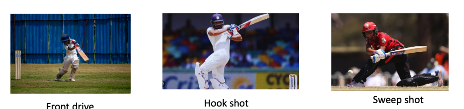
Image classification using Deep Learning has been around for almost a decade. In fact, this field with the use of Convolutional Neural Networks (CNN) is quite mature and the algorithms work very well in image classification, object detection, facial recognition and self-driving cars. In this post, I use AI image classification to identify cricketing shots. While the problem falls in a well known domain, the application of image classification in identifying cricketing shots is probably new. I have selected three cricketing shots, namely, the front drive, sweep shot, and the hook shot for this purpose. My purpose was to build a proof-of-concept and not a perfect product. I have kept the dataset deliberately small (for obvious reasons) of just about 14 samples for each cricketing shot, and for a total of about 41 total samples for both training and test data. Anyway, I get a reasonable performance from the AI model.
Included below are some examples of the data set
This post is based on this or on Image classification from Hugging face. Interestingly, this, the model used here is based on Vision Transformers (ViT from Google Brain) and not on Convolutional Neural Networks as is usually done.
The steps are to fine-tune ViT Transformer with the ‘strokes’ dataset are
- Install the necessary libraries
! pip install transformers[torch] datasets evaluate accelerate -U
! pip install -U accelerate
! pip install -U transformers
b) Login to Hugging Face account
 from huggingface_hub import notebook_login
notebook_login()

Login successful
c) Load the batting strokes dataset with 41 images
from datasets import load_dataset
df1 = load_dataset("tvganesh/strokes",split='train')
type(df1)
len(df1)

41
df1
Dataset({
features: ['image', 'label'],
num_rows: 41
})d) Create a dictionary that maps the label name to an integer and vice versa. Display the labels
labels = df1.features["label"].names
label2id, id2label = dict(), dict()
for i, label in enumerate(labels):
label2id[label] = str(i)
id2label[str(i)] = label

labels

['front drive', 'hook shot', 'sweep shot']
e) Load ViT image processor. To apply the correct transformations, ImageProcessor is initialised with a configuration that was saved along with the pretrained model
from transformers import AutoImageProcessor

checkpoint = "google/vit-base-patch16-224-in21k"
image_processor = AutoImageProcessor.from_pretrained(checkpoint)
f) Apply image transformations to the images to make the model more robust against overfitting
from torchvision.transforms import RandomResizedCrop, Compose, Normalize, ToTensor

normalize = Normalize(mean=image_processor.image_mean, std=image_processor.image_std)
size = (
    image_processor.size["shortest_edge"]
    if "shortest_edge" in image_processor.size
    else (image_processor.size["height"], image_processor.size["width"])
)
_transforms = Compose([RandomResizedCrop(size), ToTensor(), normalize])
g) Create a preprocessing function to apply the transforms and return pixel_values of the image as the inputs to the model – :
def transforms(examples):
    examples["pixel_values"] = [_transforms(img.convert("RGB")) for img in examples["image"]]
    del examples["image"]
    return examples
h) Apply the preprocessing function over the entire dataset, using Hugging Face Dataset’s ‘with_transform’ method
df1 = df1.with_transform(transforms)from transformers import DefaultDataCollator
data_collator = DefaultDataCollator()i) Evaluate model’s performance with evaluate
import evaluate
accuracy = evaluate.load("accuracy")
j) Calculate accuracy by passing in predictions and labels
import numpy as np
def compute_metrics(eval_pred):
    predictions, labels = eval_pred
    predictions = np.argmax(predictions, axis=1)
    return accuracy.compute(predictions=predictions, references=labels)
k) Load ViT by specifying the number of labels along with the number of expected labels, and the label mapping
 from transformers import AutoModelForImageClassification, TrainingArguments, Trainer

model = AutoModelForImageClassification.from_pretrained(
    checkpoint,
    num_labels=len(labels),
    id2label=id2label,
    label2id=label2id,
)
l)
- Pass the training arguments to Trainer along with the model, dataset, tokenizer, data collator, and
compute_metricsfunction. - Call train() to finetune your model.
training_args = TrainingArguments(
    output_dir="data_classify",
    remove_unused_columns=False,
    evaluation_strategy="epoch",
    save_strategy="epoch",
    learning_rate=5e-5,
    per_device_train_batch_size=8,
    #gradient_accumulation_steps=4,
    per_device_eval_batch_size=6,
    num_train_epochs=20,
    warmup_ratio=0.1,
    logging_steps=10,
    load_best_model_at_end=True,
    metric_for_best_model="accuracy",
    push_to_hub=True,
)

trainer = Trainer(
    model=model,
    args=training_args,
    data_collator=data_collator,
    train_dataset=train_dataset,
    eval_dataset=test_dataset,
    tokenizer=image_processor,
    compute_metrics=compute_metrics,
)

trainer.train()

Epoch	Training Loss	Validation Loss	Accuracy
1	No log	0.434451	1.000000
2	No log	0.388312	1.000000
3	0.361200	0.409932	0.888889
4	0.361200	0.245226	1.000000
5	0.293400	0.196930	1.000000
6	0.293400	0.167858	1.000000
7	0.293400	0.140349	1.000000
8	0.203000	0.153016	1.000000
9	0.203000	0.116115	1.000000
10	0.150500	0.129171	1.000000
11	0.150500	0.103121	1.000000
12	0.150500	0.108433	1.000000
13	0.138800	0.107799	1.000000
14	0.138800	0.093700	1.000000
15	0.107600	0.100769	1.000000
16	0.107600	0.113148	1.000000
17	0.107600	0.100740	1.000000
18	0.104700	0.177483	0.888889
19	0.104700	0.084438	1.000000
20	0.090200	0.112654	1.000000
TrainOutput(global_step=80, training_loss=0.18118578270077706, metrics={'train_runtime': 176.3834, 'train_samples_per_second': 3.628, 'train_steps_per_second': 0.454, 'total_flos': 4.959531785650176e+16, 'train_loss': 0.18118578270077706, 'epoch': 20.0})
m) Push to Hub
trainer.push_to_hub()You can try out my fine-tuned model at identify_stroke̱
Here are a couple of trials
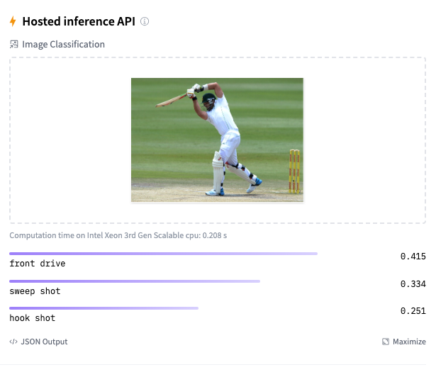
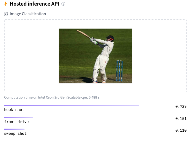
As I mentioned before, the model should be reasonably accurate but not perfect, since my training dataset is extremely small. This is just a prototype to show that shot identification in cricket with AI is in the realm of the possible.
References
Do take a look at
- Using Reinforcement Learning to solve Gridworld
- Deconstructing Convolutional Neural Networks with Tensorflow and Keras
- GenerativeAI:Using T5 Transformer model to summarise Indian Philosophy
- GooglyPlusPlus: Win Probability using Deep Learning and player embeddings
- T20 Win Probability using CTGANs, synthetic data
- Deep Learning from first principles in Python, R and Octave – Part 6
- Introducing QCSimulator: A 5-qubit quantum computing simulator in R
- Big Data 6: The T20 Dance of Apache NiFi and yorkpy
- Re-introducing cricketr! : An R package to analyze performances of cricketers
To see all posts click Index of posts


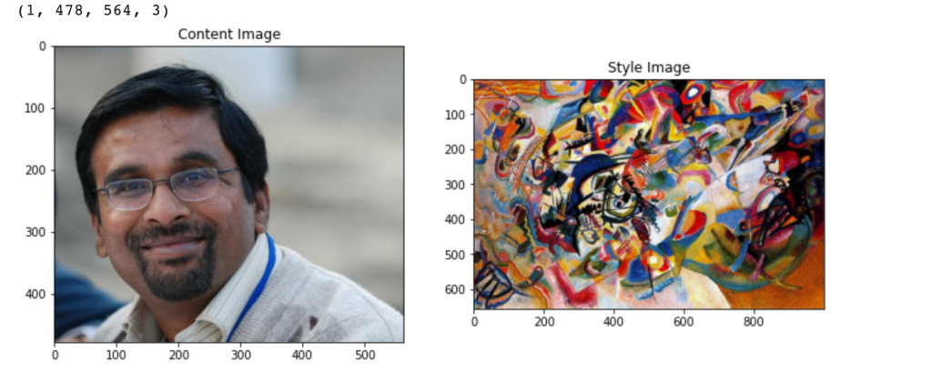
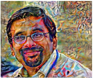
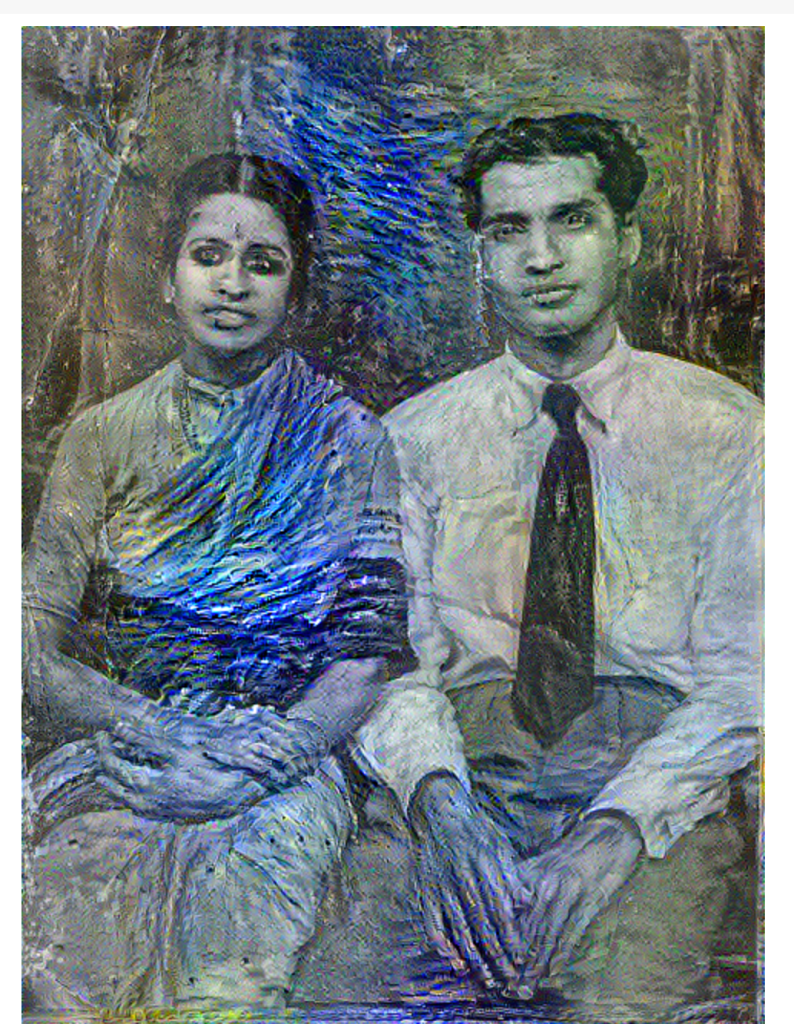
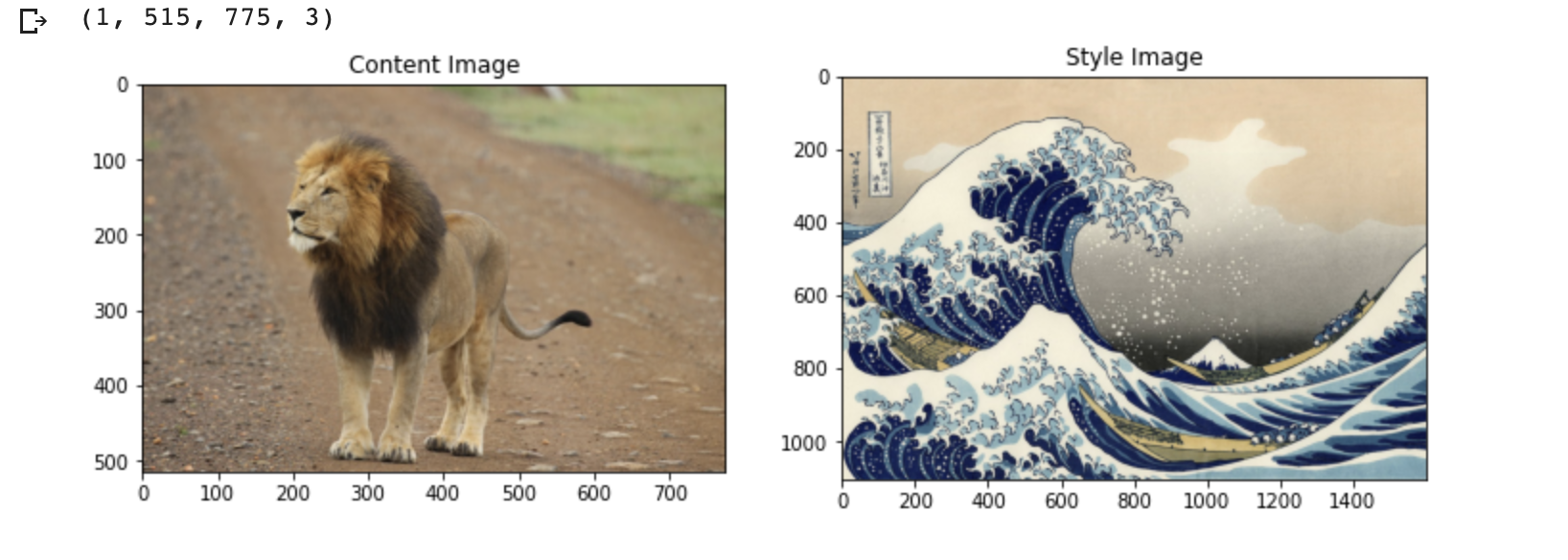
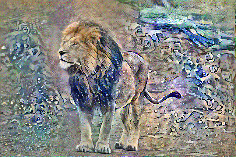
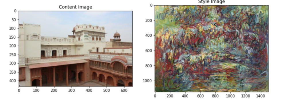
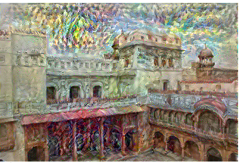
 and
and  represent the activations at layer ‘l’ in a filter i, at position ‘j’. The intuition is that the activations will be same for similar source and generated image. We need to minimise the content loss so that the generated stylized image is as close to the original image as possible. An intermediate layer of VGG19 block5_conv2 is used
 x
x 
 and width
  with
with  channels
 and
and  are the Gram matrices of the style and generated images respectively. By minimising the distance in the gram matrices of the style and generated image we can ensure that generated image is a stylized version of the original image similar to the style image