“Curiouser and curiouser!” cried Alice
“The time has come,” the walrus said, “to talk of many things: Of shoes and ships – and sealing wax – of cabbages and kings”
“Begin at the beginning,”the King said, very gravely,“and go on till you come to the end: then stop.”
“And what is the use of a book,” thought Alice, “without pictures or conversation?”
Excerpts from Alice in Wonderland by Lewis CarrollIntroduction
This post is a continuation of my previous post “Introducing cricketr! A R package to analyze the performances of cricketers.” In this post I take my package cricketr for a spin. For this analysis I focus on the Indian batting legends
– Sachin Tendulkar (Master Blaster)
– Rahul Dravid (The Will)
– Sourav Ganguly ( The Dada Prince)
– Sunil Gavaskar (Little Master)
This post is also hosted on RPubs – cricketr-1
If you are passionate about cricket, and love analyzing cricket performances, then check out my 2 racy books on cricket! In my books, I perform detailed yet compact analysis of performances of both batsmen, bowlers besides evaluating team & match performances in Tests , ODIs, T20s & IPL. You can buy my books on cricket from Amazon at $12.99 for the paperback and $4.99/$6.99 respectively for the kindle versions. The books can be accessed at Cricket analytics with cricketr and Beaten by sheer pace-Cricket analytics with yorkr A must read for any cricket lover! Check it out!!
You can download the latest PDF version of the book at ‘Cricket analytics with cricketr and cricpy: Analytics harmony with R and Python-6th edition‘
d $4.99/Rs 320 and $6.99/Rs448 respectively
Important note 1: The latest release of ‘cricketr’ now includes the ability to analyze performances of teams now!! See Cricketr adds team analytics to its repertoire!!!
Important note 2 : Cricketr can now do a more fine-grained analysis of players, see Cricketr learns new tricks : Performs fine-grained analysis of players
Important note 3: Do check out the python avatar of cricketr, ‘cricpy’ in my post ‘Introducing cricpy:A python package to analyze performances of cricketers”
(Do check out my interactive Shiny app implementation using the cricketr package – Sixer – R package cricketr’s new Shiny avatar)
Note: If you would like to do a similar analysis for a different set of batsman and bowlers, you can clone/download my skeleton cricketr template from Github (which is the R Markdown file I have used for the analysis below). You will only need to make appropriate changes for the players you are interested in. Just a familiarity with R and R Markdown only is needed.
The package can be installed directly from CRAN
if (!require("cricketr")){
    install.packages("cricketr",lib = "c:/test")
}
library(cricketr)
or from Github
library(devtools)
install_github("tvganesh/cricketr")
library(cricketr)
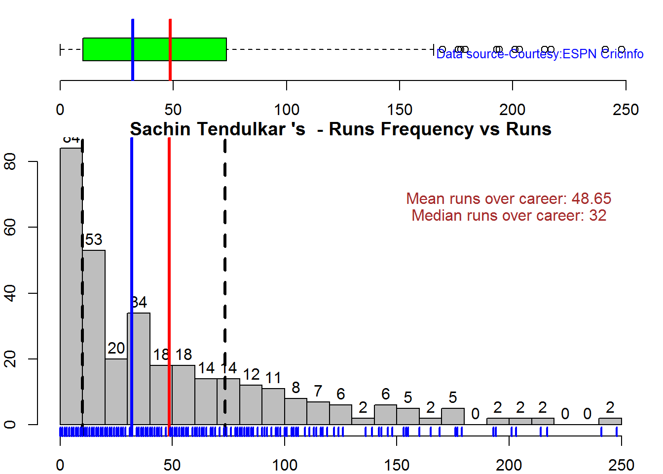
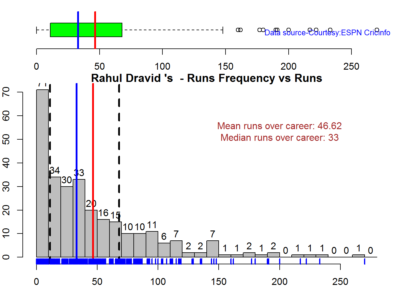
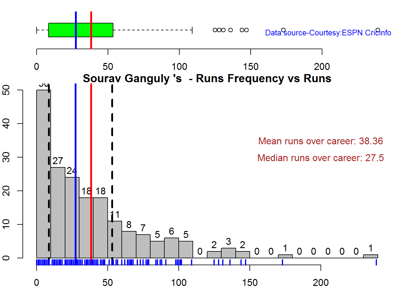
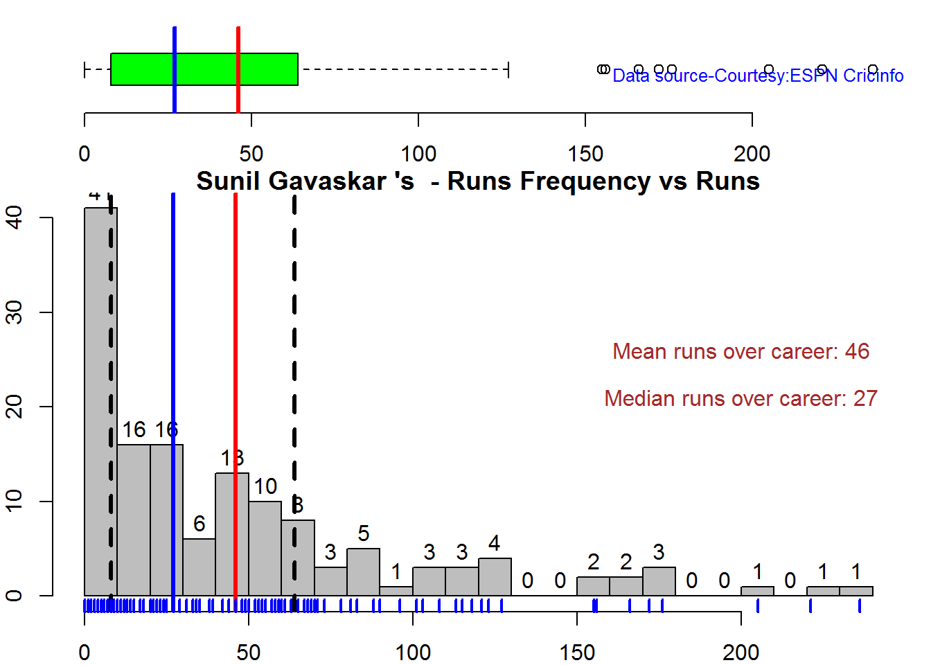
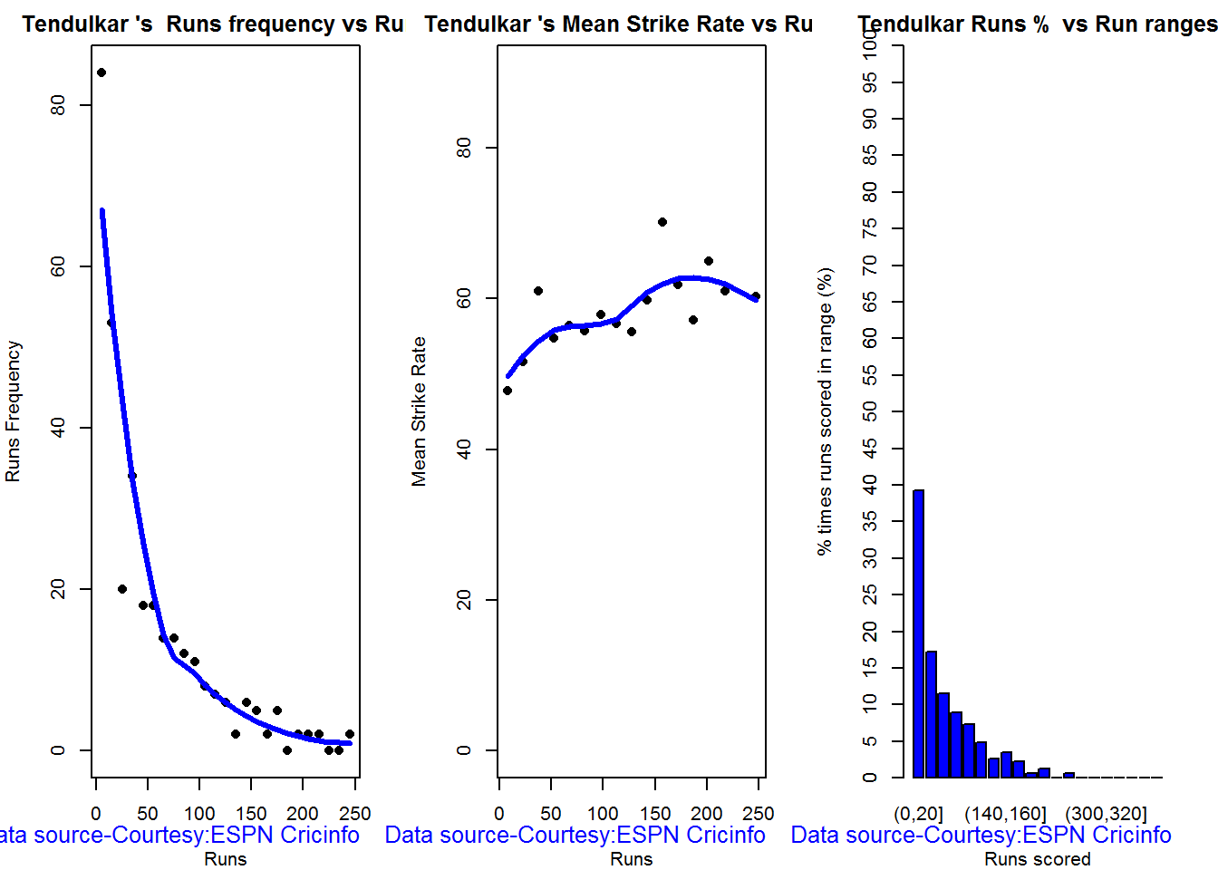
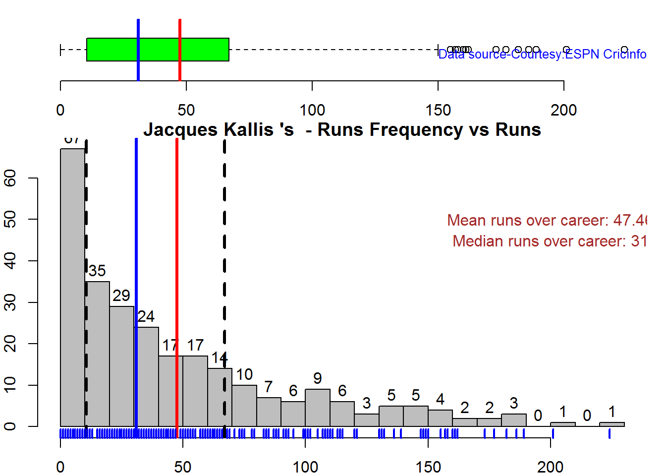
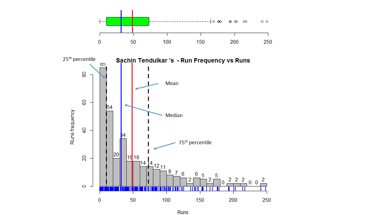
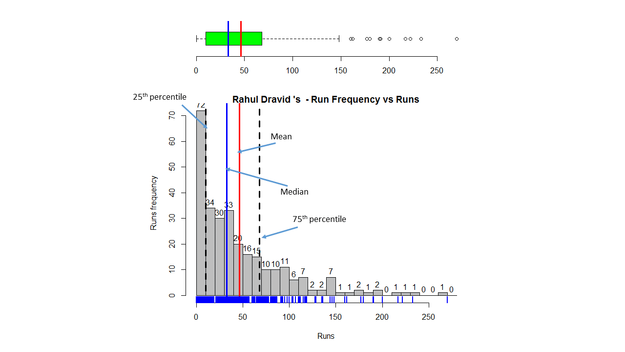
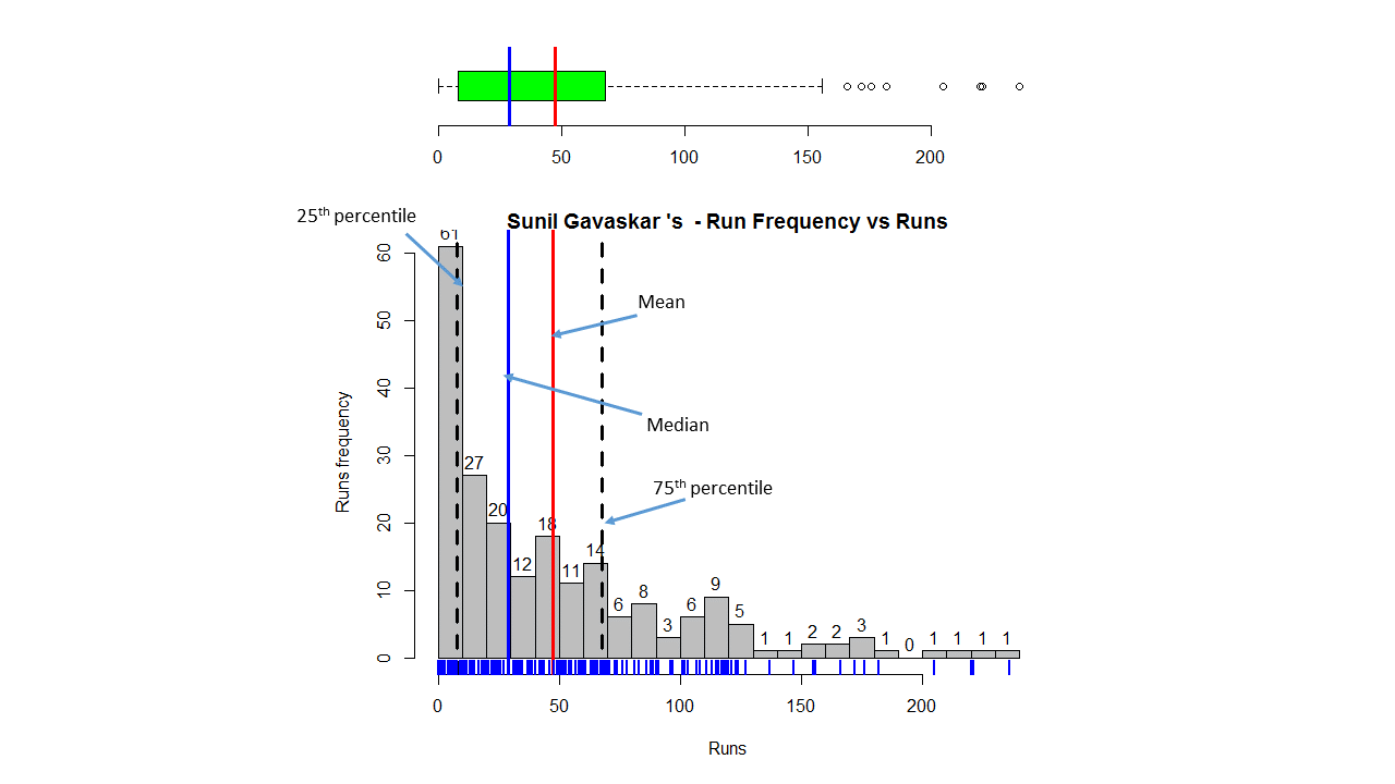
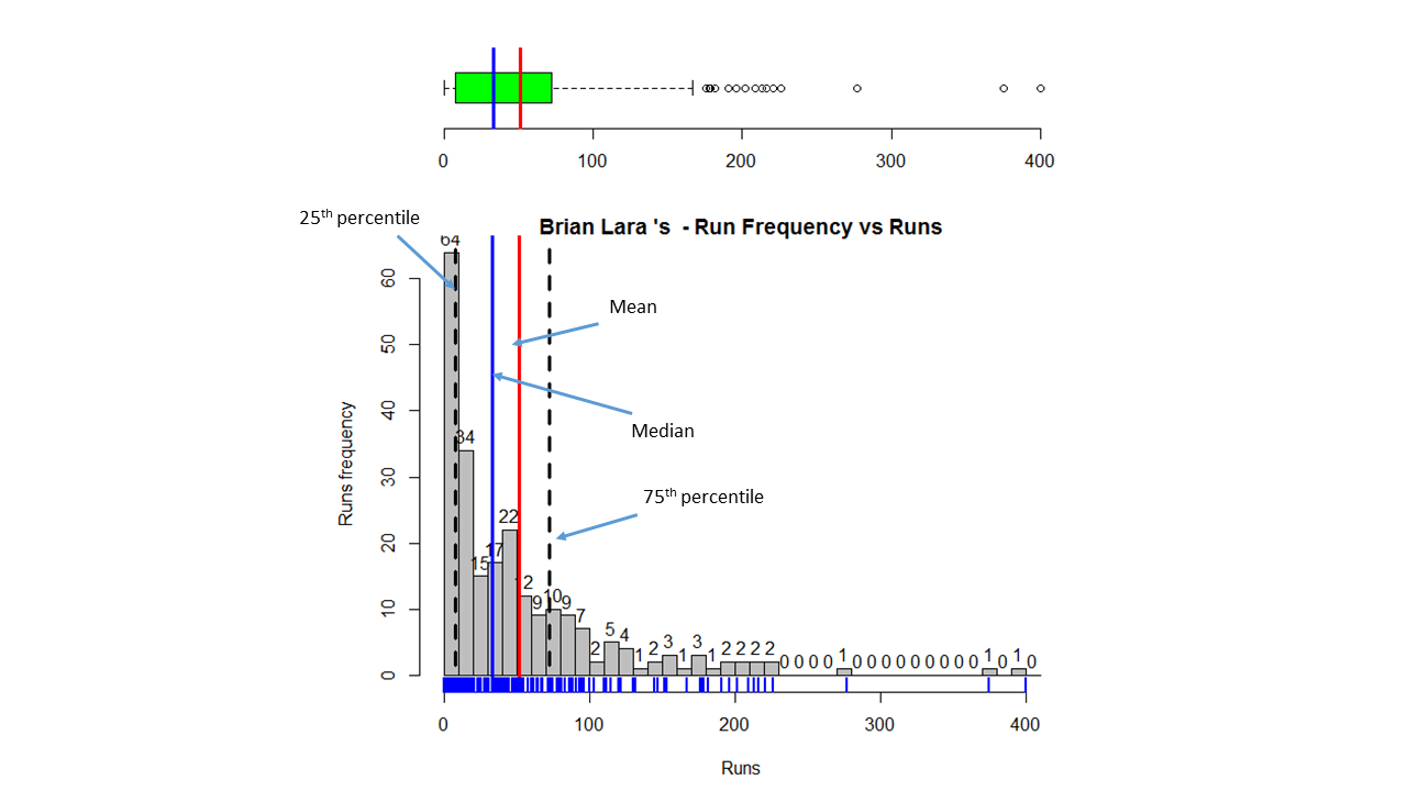
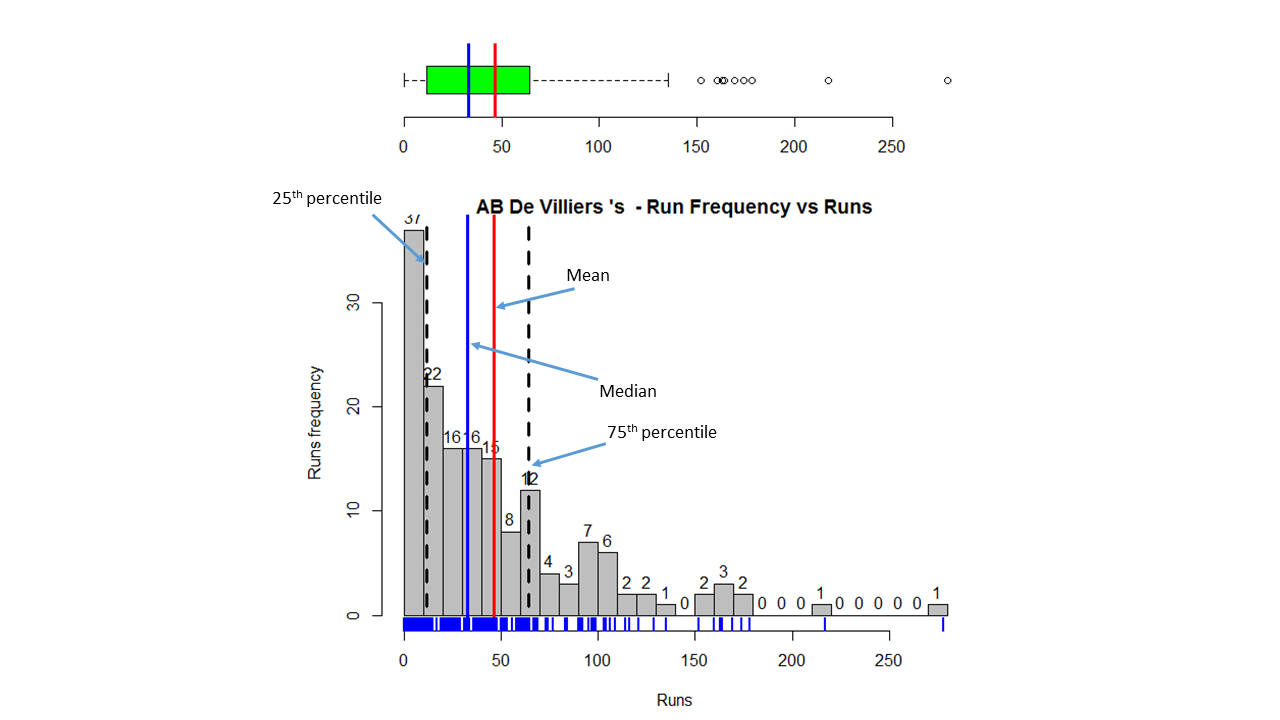
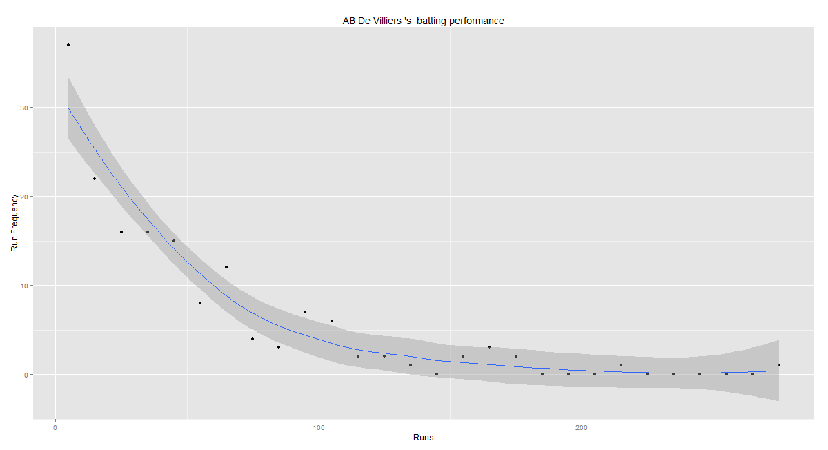
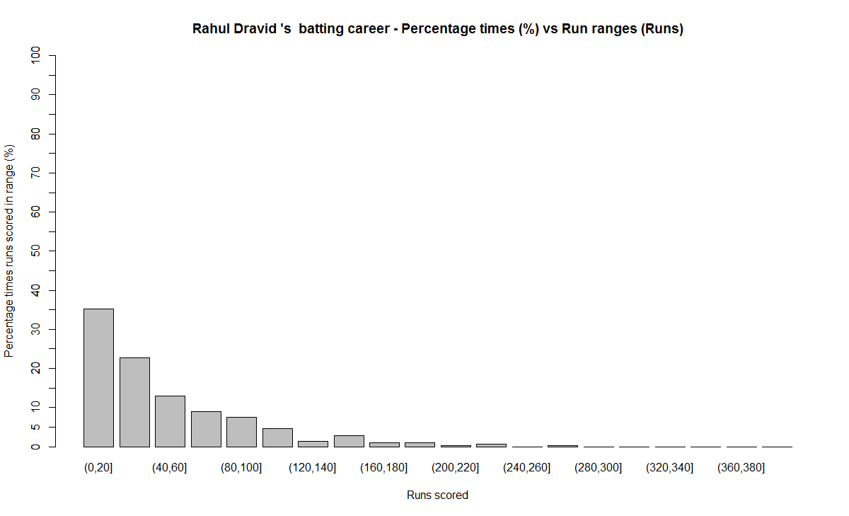
Box Histogram Plot
This plot shows a combined boxplot of the Runs ranges and a histogram of the Runs Frequency The plot below indicate the Tendulkar’s average is the highest. He is followed by Dravid, Gavaskar and then Ganguly
batsmanPerfBoxHist("./tendulkar.csv","Sachin Tendulkar")

batsmanPerfBoxHist("./dravid.csv","Rahul Dravid")

batsmanPerfBoxHist("./ganguly.csv","Sourav Ganguly")

batsmanPerfBoxHist("./gavaskar.csv","Sunil Gavaskar")
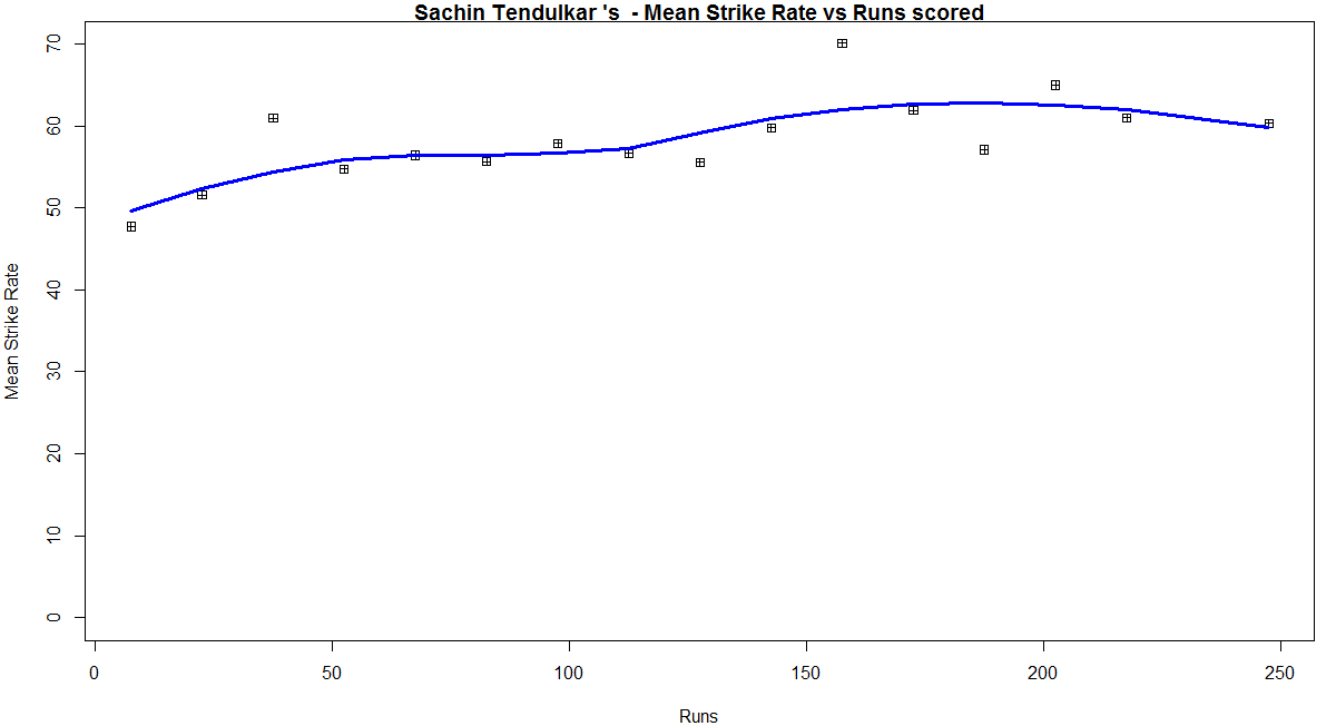
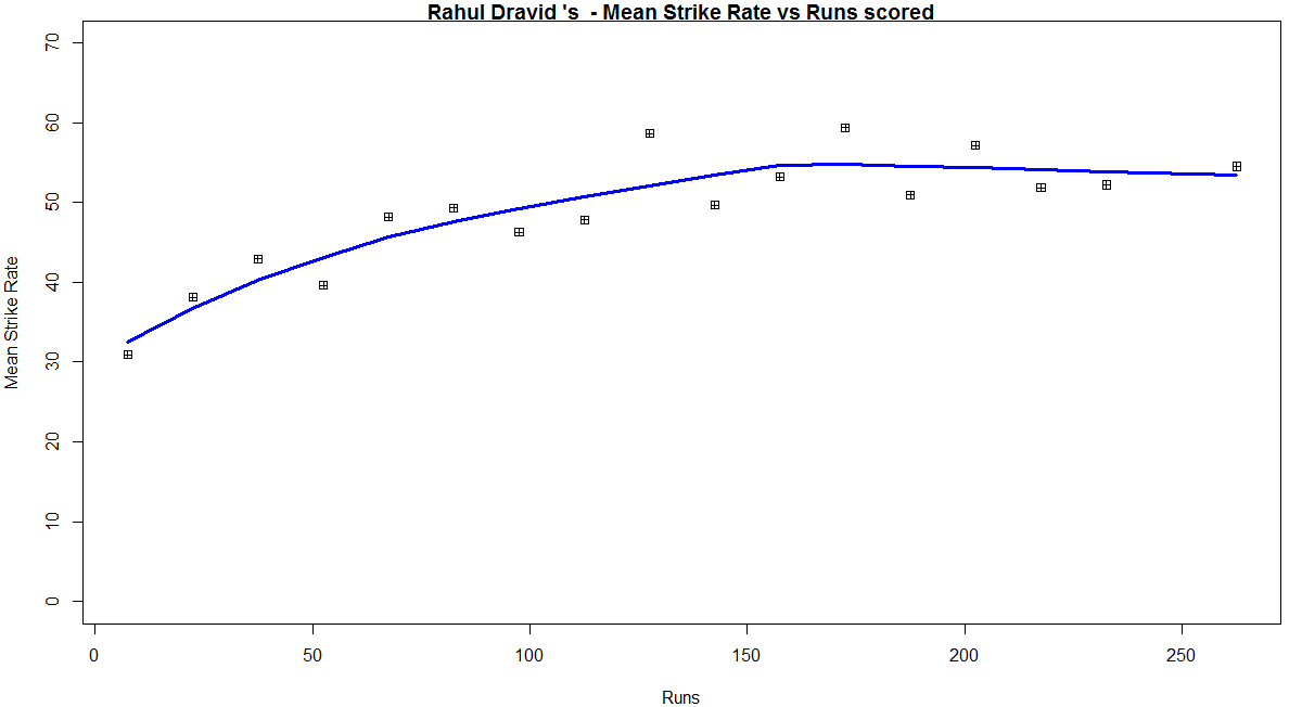
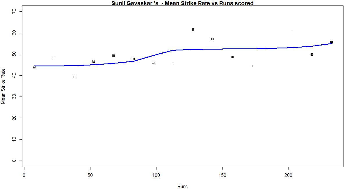
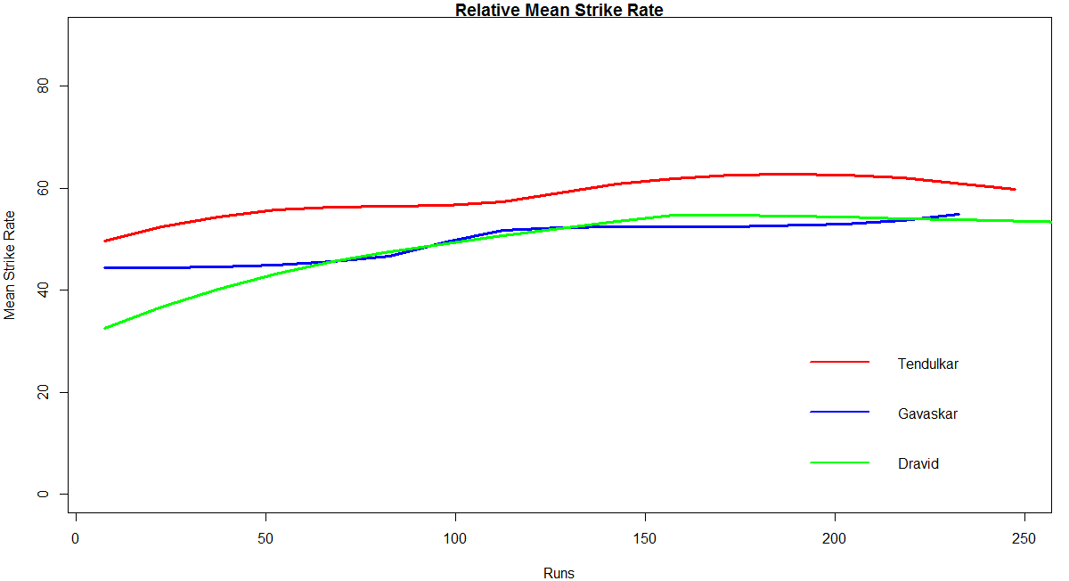
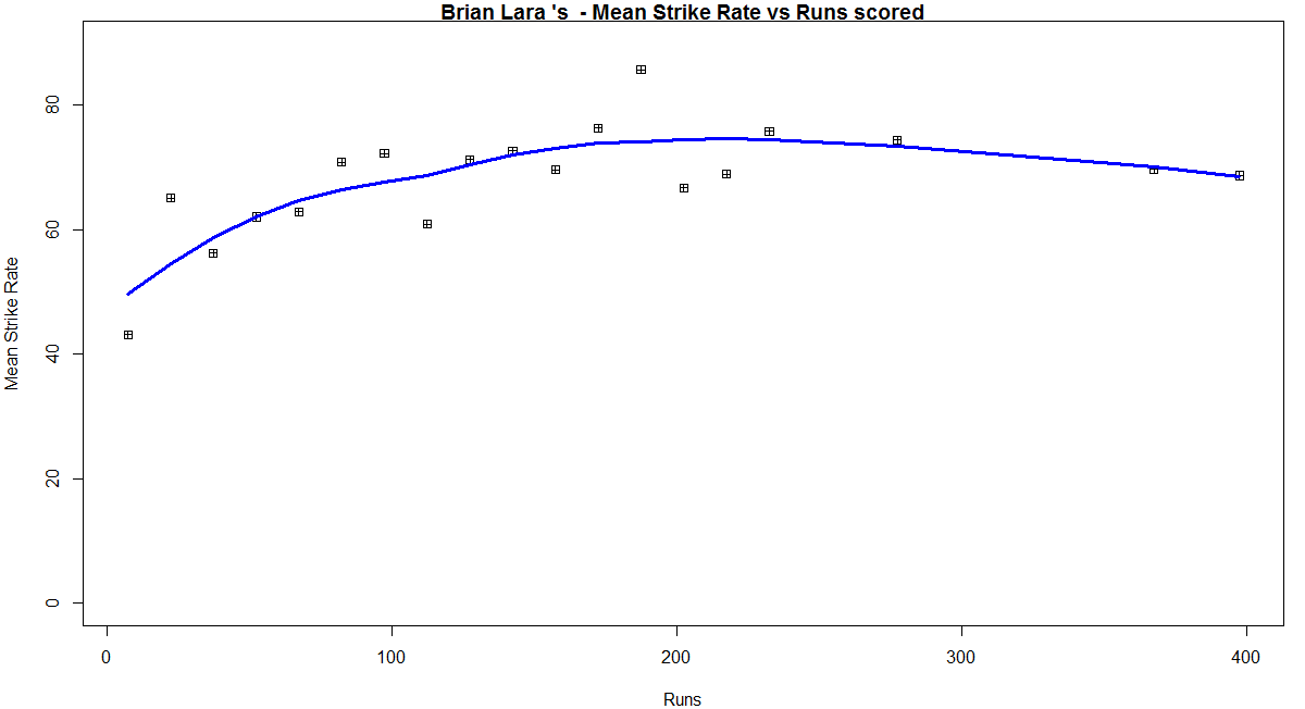
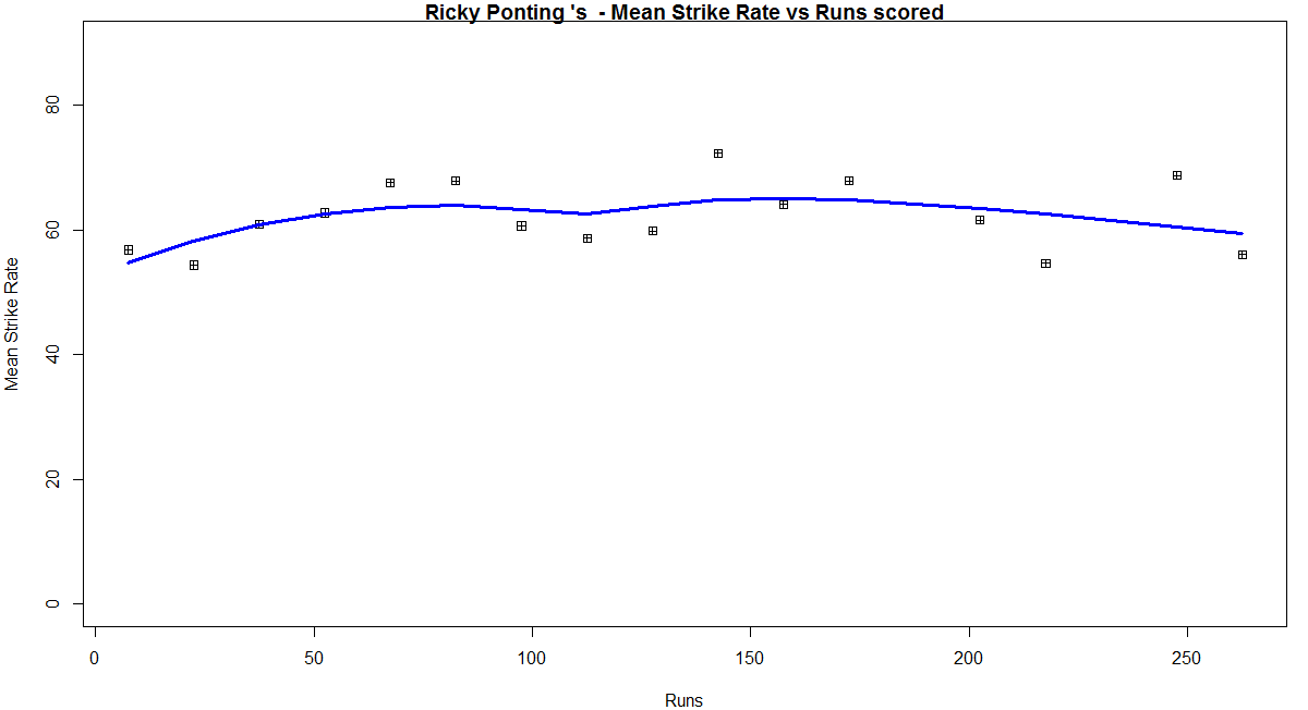
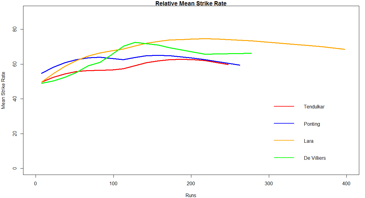
Relative Mean Strike Rate
In this first plot I plot the Mean Strike Rate of the batsmen. Tendulkar leads in the Mean Strike Rate for each runs in the range 100- 180. Ganguly has a very good Mean Strike Rate for runs range 40 -80
frames <- list("./tendulkar.csv","./dravid.csv","ganguly.csv","gavaskar.csv")
names <- list("Tendulkar","Dravid","Ganguly","Gavaskar")
relativeBatsmanSR(frames,names)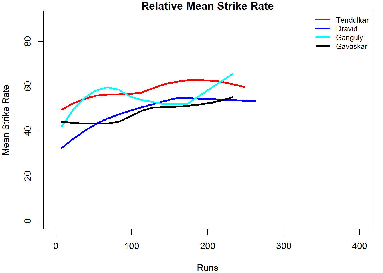
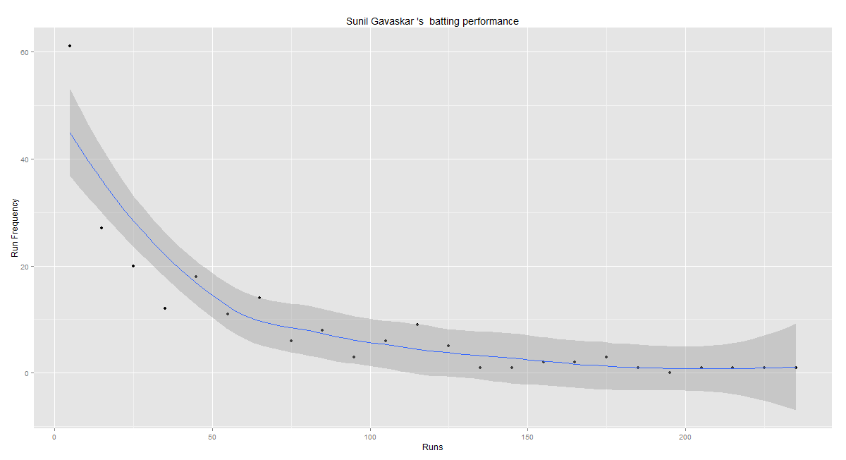
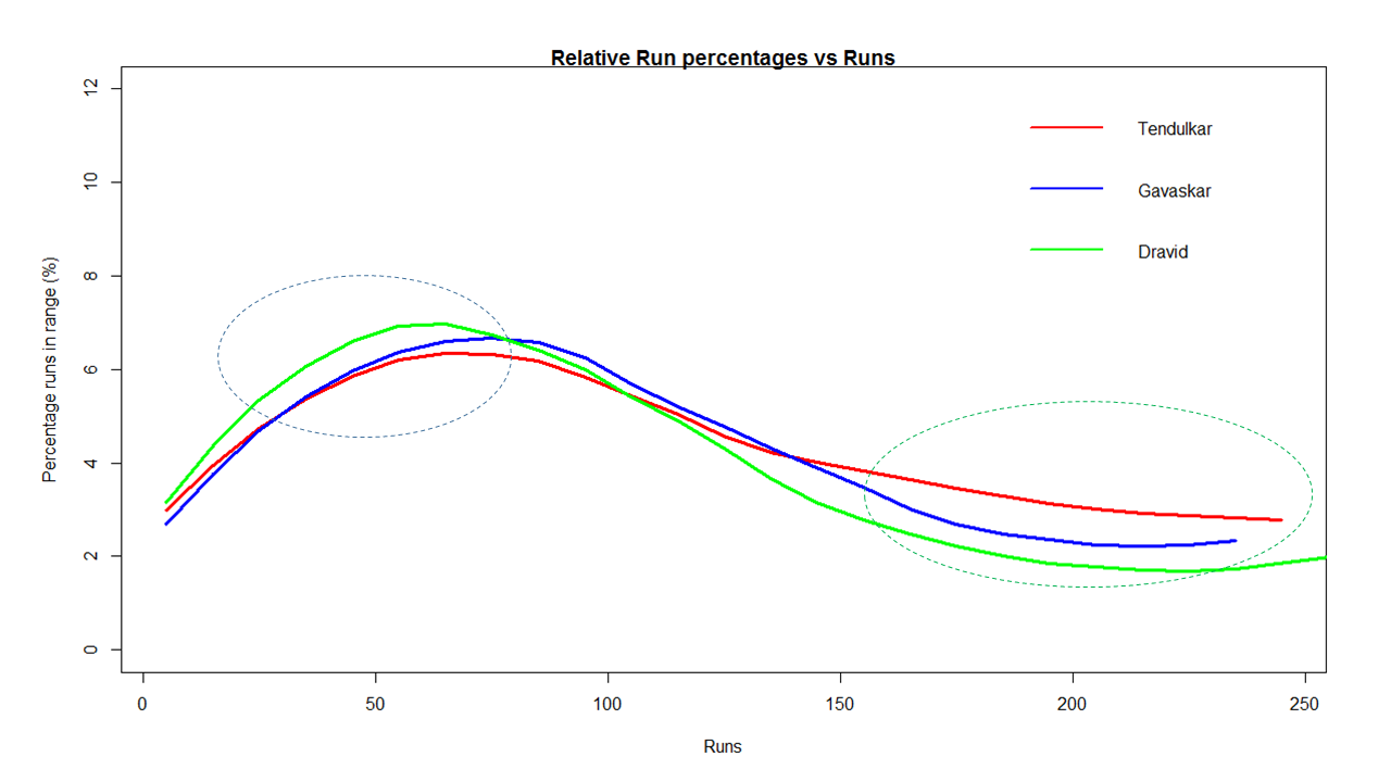
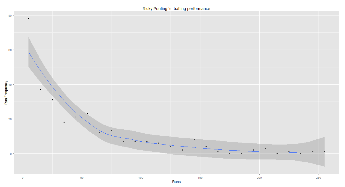
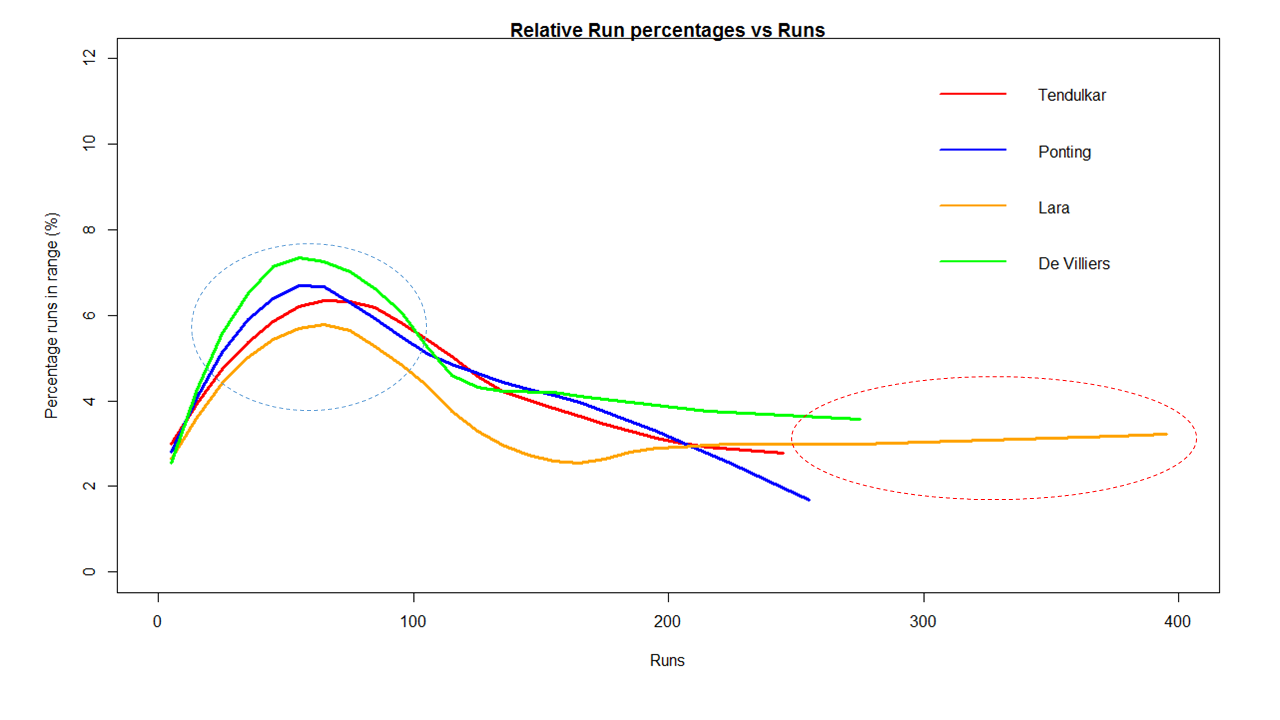
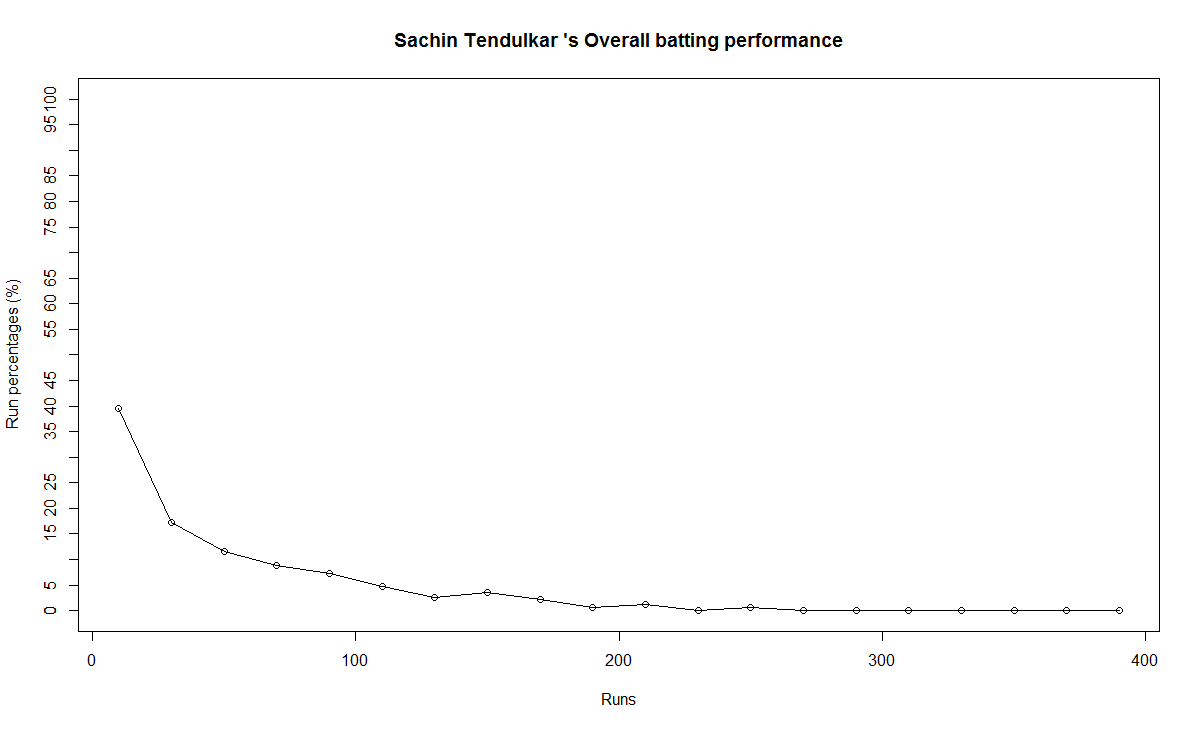
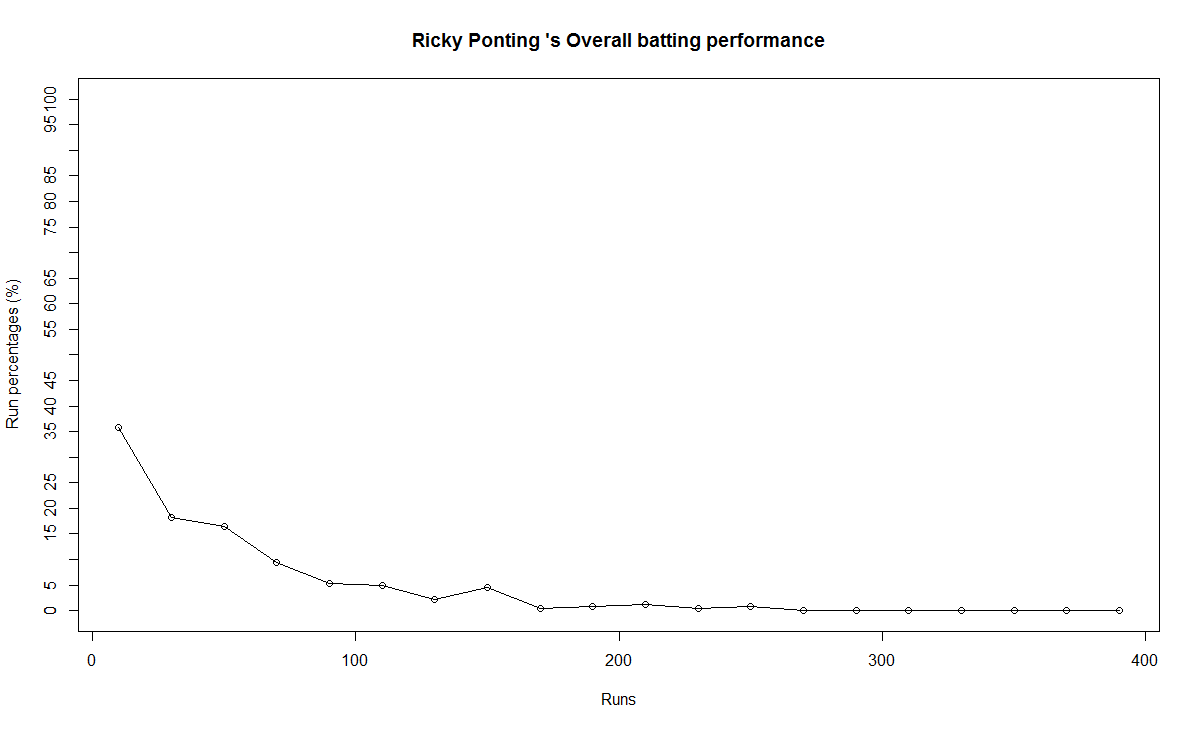
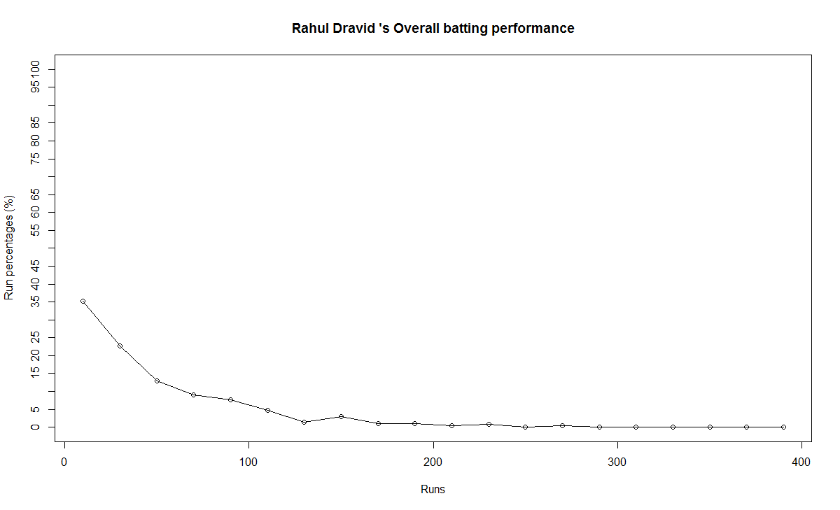
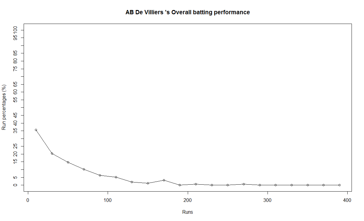
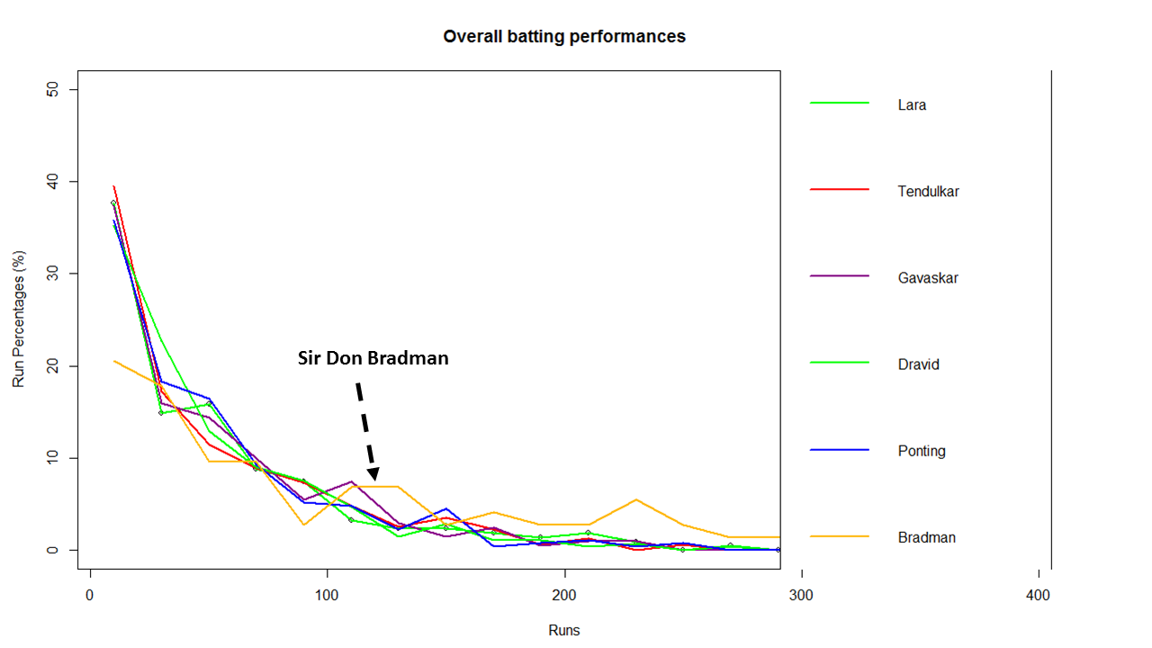
Relative Runs Frequency Percentage
The plot below show the percentage contribution in each 10 runs bucket over the entire career.The percentage Runs Frequency is fairly close but Gavaskar seems to lead most of the way
frames <- list("./tendulkar.csv","./dravid.csv","ganguly.csv","gavaskar.csv")
names <- list("Tendulkar","Dravid","Ganguly","Gavaskar")
relativeRunsFreqPerf(frames,names)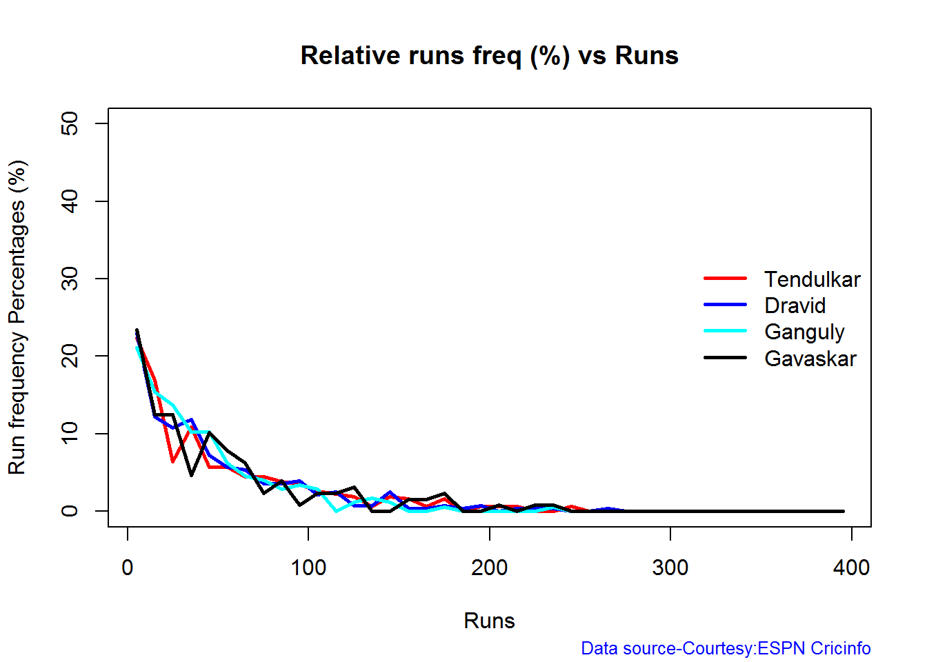
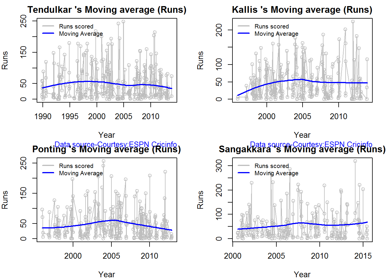
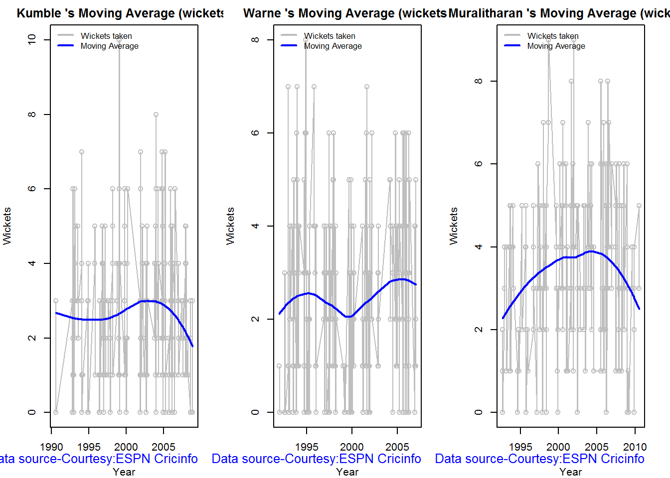
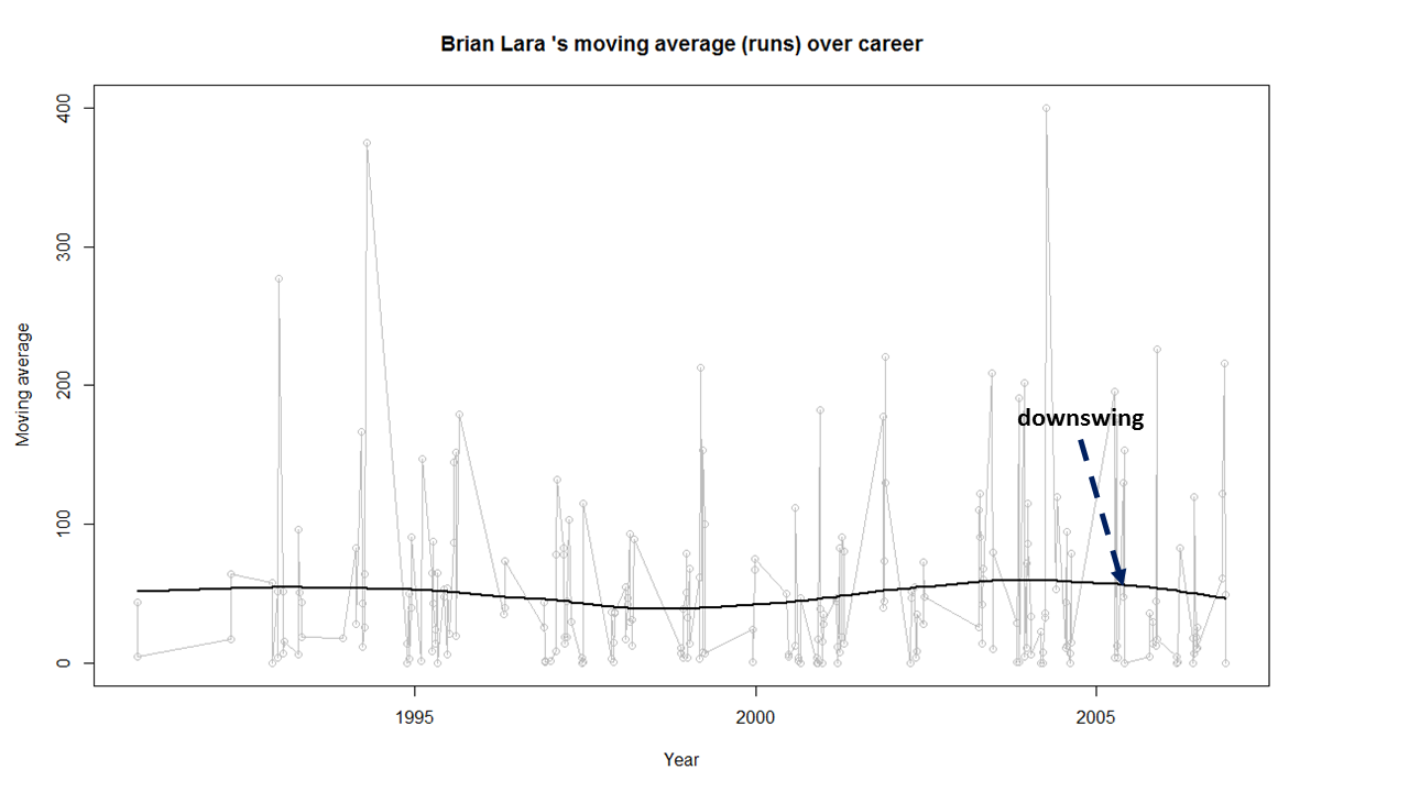
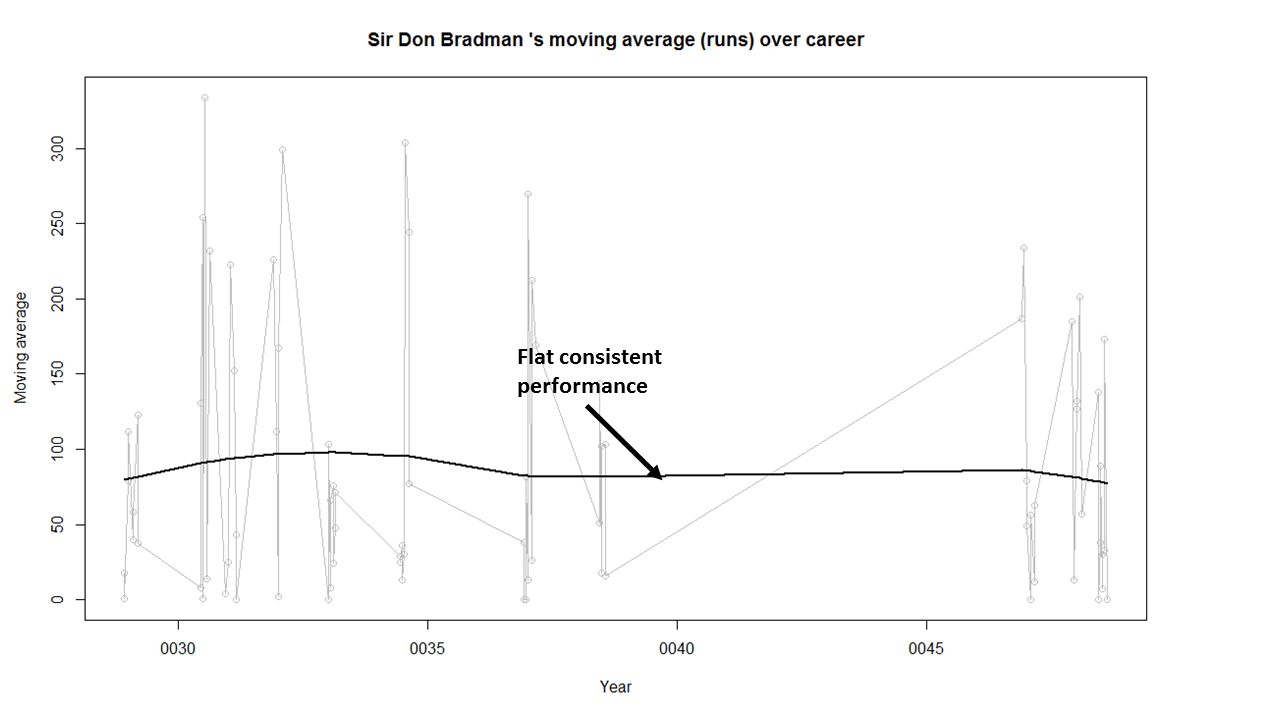
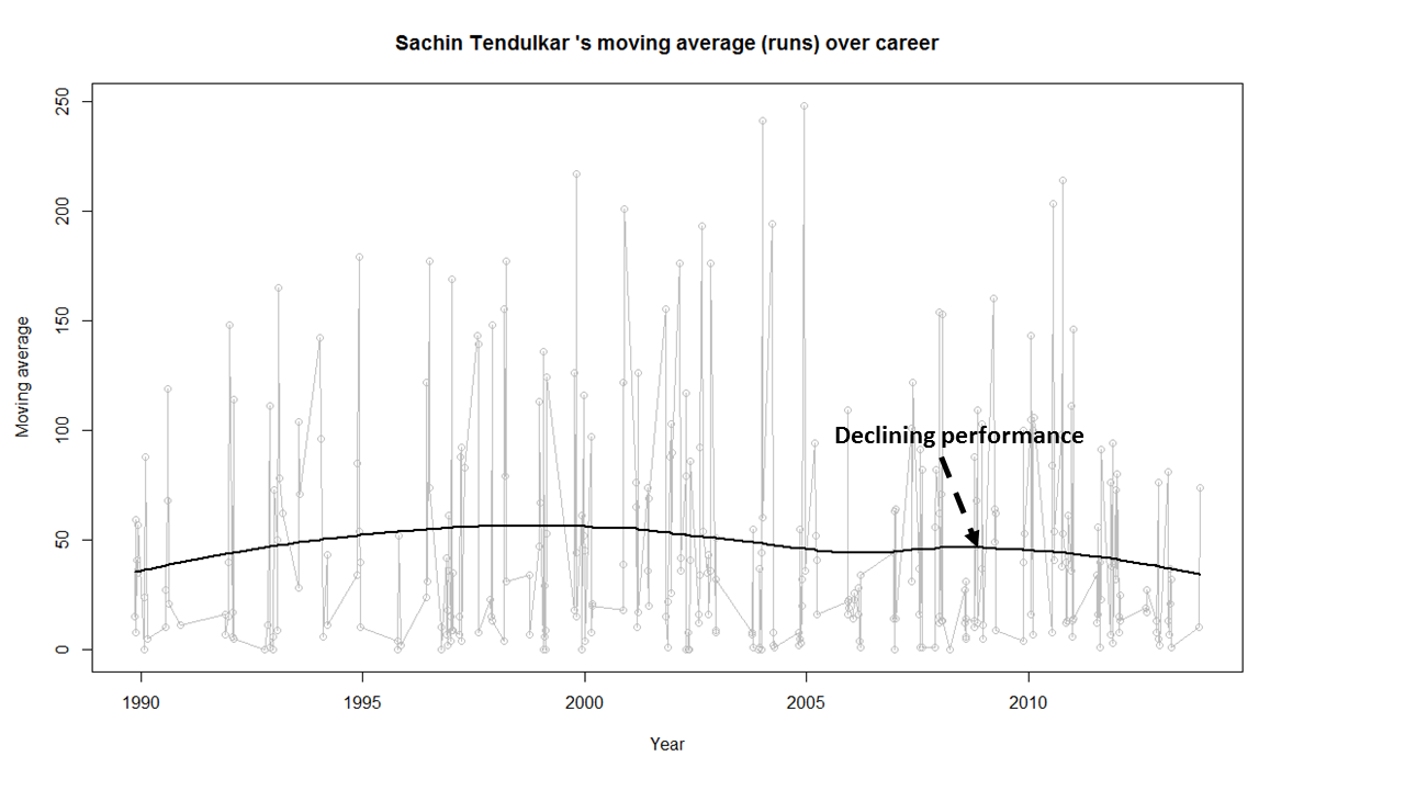
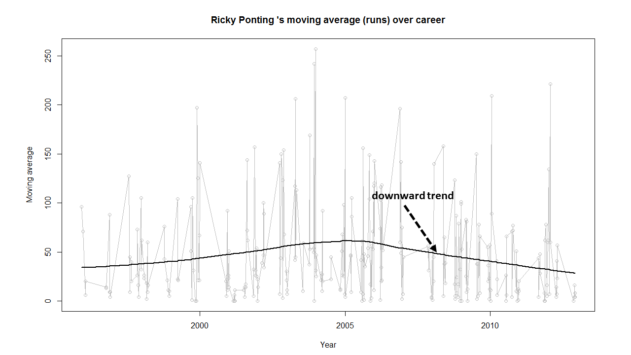
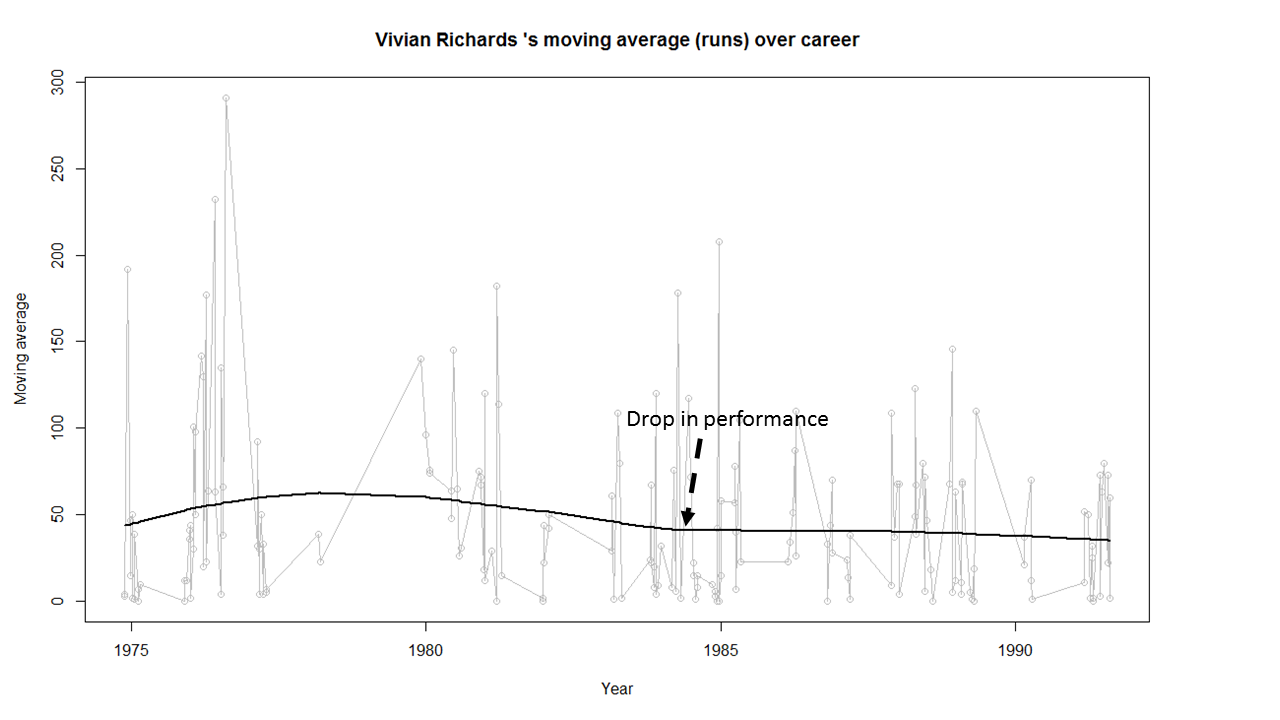
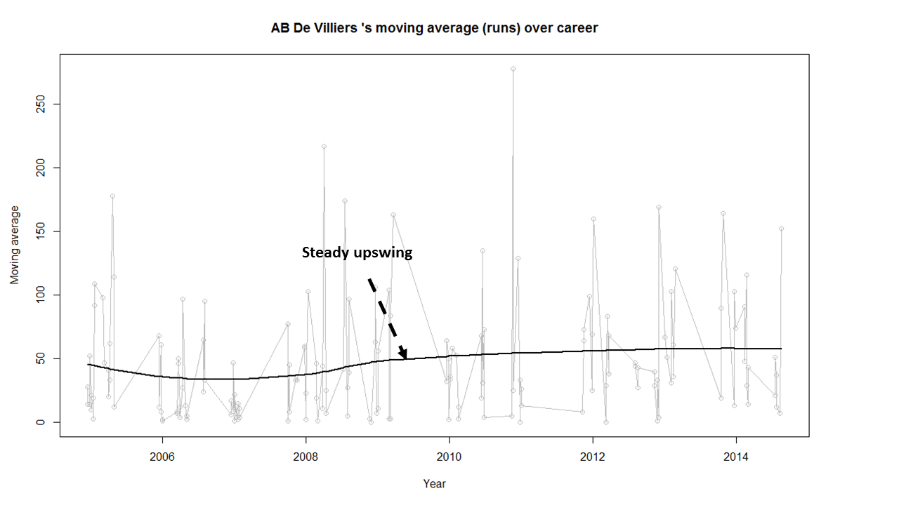
Moving Average of runs over career
The moving average for the 4 batsmen indicate the following – Tendulkar and Ganguly’s career has a downward trend and their retirement didn’t come too soon – Dravid and Gavaskar’s career definitely shows an upswing. They probably had a year or two left.
par(mfrow=c(2,2))
par(mar=c(4,4,2,2))
batsmanMovingAverage("./tendulkar.csv","Tendulkar")
batsmanMovingAverage("./dravid.csv","Dravid")
batsmanMovingAverage("./ganguly.csv","Ganguly")
batsmanMovingAverage("./gavaskar.csv","Gavaskar")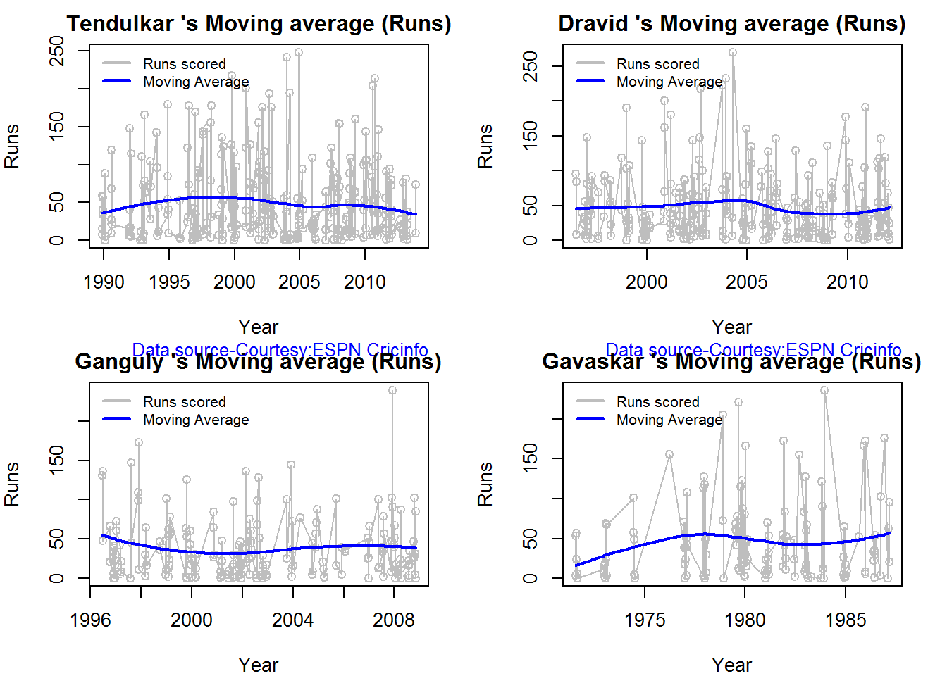
dev.off()## null device
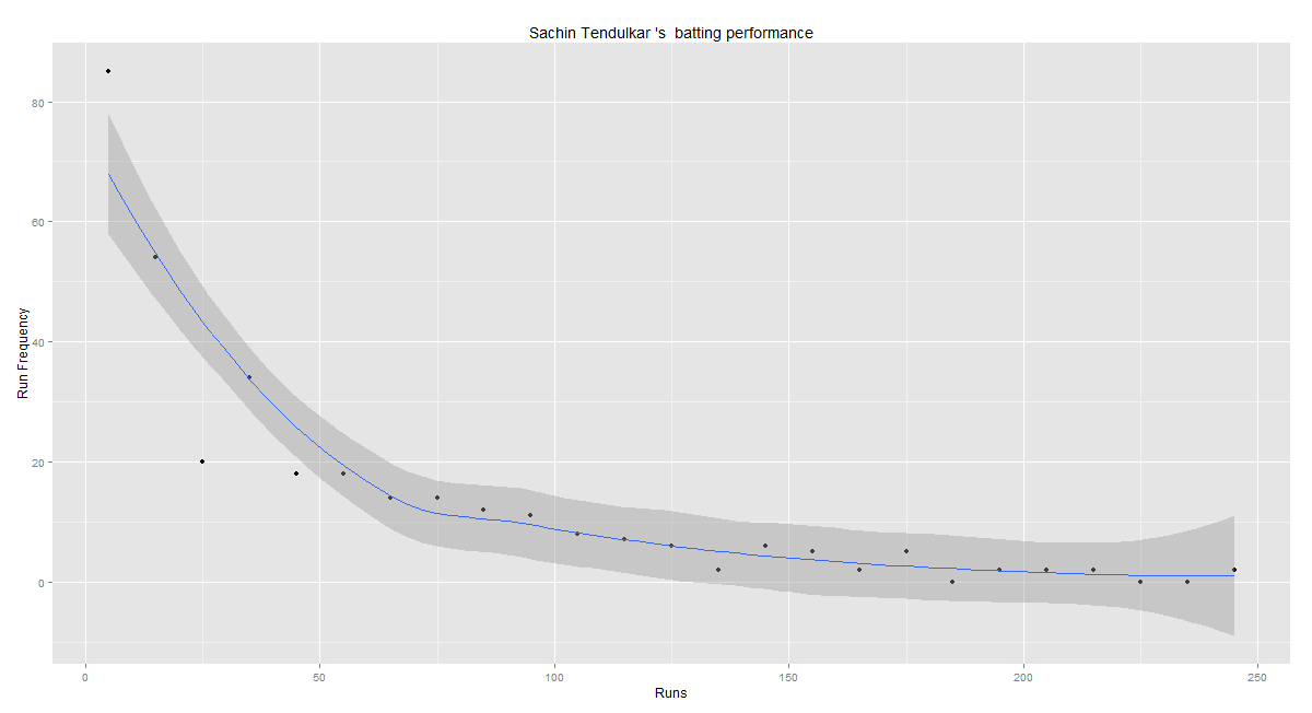
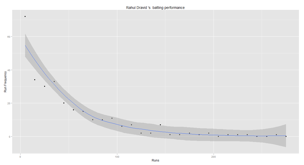
## 1Runs forecast
The forecast for the batsman is shown below. The plots indicate that only Tendulkar seemed to maintain a consistency over the period while the rest seem to score less than their forecasted runs in the last 10% of the career
par(mfrow=c(2,2))
par(mar=c(4,4,2,2))
batsmanPerfForecast("./tendulkar.csv","Sachin Tendulkar")
batsmanPerfForecast("./dravid.csv","Rahul Dravid")
batsmanPerfForecast("./ganguly.csv","Sourav Ganguly")
batsmanPerfForecast("./gavaskar.csv","Sunil Gavaskar")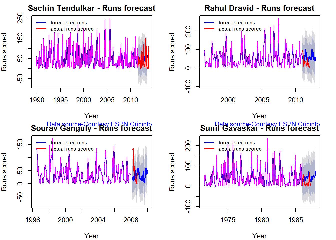
dev.off()## null device
## 1Check for batsman in-form/out-of-form
The following snippet checks whether the batsman is in-inform or ouyt-of-form during the last 10% innings of the career. This is done by choosing the null hypothesis (h0) to indicate that the batsmen are in-form. Ha is the alternative hypothesis that they are not-in-form. The population is based on the 1st 90% of career runs. The last 10% is taken as the sample and a check is made on the lower tail to see if the sample mean is less than 95% confidence interval. If this difference is >0.05 then the batsman is considered out-of-form.
The computation show that Tendulkar was out-of-form while the other’s weren’t. While Dravid and Gavaskar’s moving average do show an upward trend the surprise is Ganguly. This could be that Ganguly was able to keep his average in the last 10% to with the 95$ confidence interval. It has to be noted that Ganguly’s average was much lower than Tendulkar
checkBatsmanInForm("./tendulkar.csv","Tendulkar")## *******************************************************************************************
##
## Population size: 294 Mean of population: 50.48
## Sample size: 33 Mean of sample: 32.42 SD of sample: 29.8
##
## Null hypothesis H0 : Tendulkar 's sample average is within 95% confidence interval
## of population average
## Alternative hypothesis Ha : Tendulkar 's sample average is below the 95% confidence
## interval of population average
##
## [1] "Tendulkar 's Form Status: Out-of-Form because the p value: 0.000713 is less than alpha= 0.05"
## *******************************************************************************************checkBatsmanInForm("./dravid.csv","Dravid")## *******************************************************************************************
##
## Population size: 256 Mean of population: 46.98
## Sample size: 29 Mean of sample: 43.48 SD of sample: 40.89
##
## Null hypothesis H0 : Dravid 's sample average is within 95% confidence interval
## of population average
## Alternative hypothesis Ha : Dravid 's sample average is below the 95% confidence
## interval of population average
##
## [1] "Dravid 's Form Status: In-Form because the p value: 0.324138 is greater than alpha= 0.05"
## *******************************************************************************************checkBatsmanInForm("./ganguly.csv","Ganguly")## *******************************************************************************************
##
## Population size: 169 Mean of population: 38.94
## Sample size: 19 Mean of sample: 33.21 SD of sample: 32.97
##
## Null hypothesis H0 : Ganguly 's sample average is within 95% confidence interval
## of population average
## Alternative hypothesis Ha : Ganguly 's sample average is below the 95% confidence
## interval of population average
##
## [1] "Ganguly 's Form Status: In-Form because the p value: 0.229006 is greater than alpha= 0.05"
## *******************************************************************************************checkBatsmanInForm("./gavaskar.csv","Gavaskar")## *******************************************************************************************
##
## Population size: 125 Mean of population: 44.67
## Sample size: 14 Mean of sample: 57.86 SD of sample: 58.55
##
## Null hypothesis H0 : Gavaskar 's sample average is within 95% confidence interval
## of population average
## Alternative hypothesis Ha : Gavaskar 's sample average is below the 95% confidence
## interval of population average
##
## [1] "Gavaskar 's Form Status: In-Form because the p value: 0.793276 is greater than alpha= 0.05"
## *******************************************************************************************dev.off()## null device
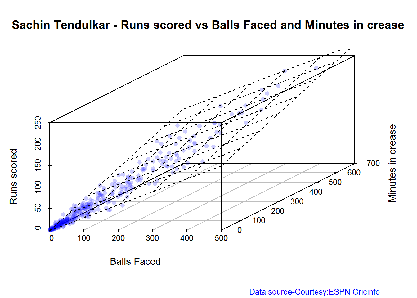
## 13D plot of Runs vs Balls Faced and Minutes at Crease
The plot is a scatter plot of Runs vs Balls faced and Minutes at Crease. A prediction plane is fitted
par(mfrow=c(1,2))
par(mar=c(4,4,2,2))
battingPerf3d("./tendulkar.csv","Tendulkar")
battingPerf3d("./dravid.csv","Dravid")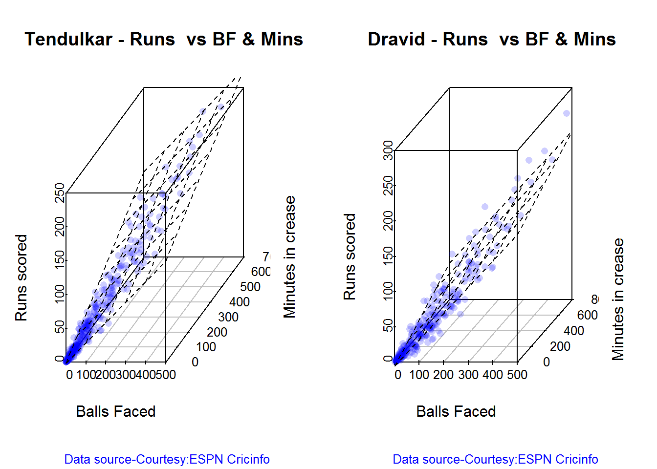
par(mfrow=c(1,2))
par(mar=c(4,4,2,2))
battingPerf3d("./ganguly.csv","Ganguly")
battingPerf3d("./gavaskar.csv","Gavaskar")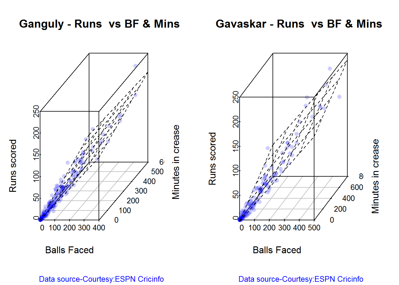
dev.off()## null device
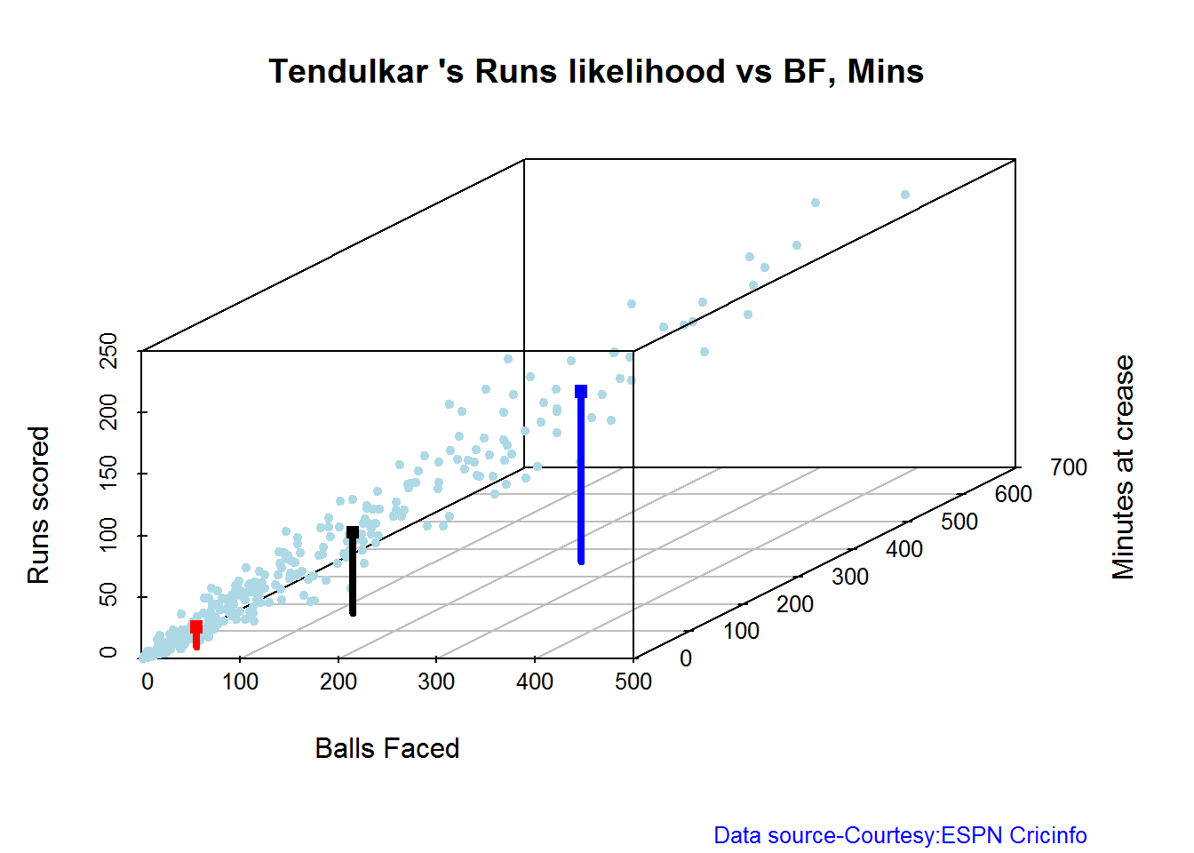
## 1Predicting Runs given Balls Faced and Minutes at Crease
A multi-variate regression plane is fitted between Runs and Balls faced +Minutes at crease.
BF <- seq( 10, 400,length=15)
Mins <- seq(30,600,length=15)
newDF <- data.frame(BF,Mins)
tendulkar <- batsmanRunsPredict("./tendulkar.csv","Tendulkar",newdataframe=newDF)
dravid <- batsmanRunsPredict("./dravid.csv","Dravid",newdataframe=newDF)
ganguly <- batsmanRunsPredict("./ganguly.csv","Ganguly",newdataframe=newDF)
gavaskar <- batsmanRunsPredict("./gavaskar.csv","Gavaskar",newdataframe=newDF)
The fitted model is then used to predict the runs that the batsmen will score for a given Balls faced and Minutes at crease. It can be seen Tendulkar has a much higher Runs scored than all of the others.
Tendulkar is followed by Ganguly who we saw earlier had a very good strike rate. However it must be noted that Dravid and Gavaskar have a better average.
batsmen <-cbind(round(tendulkar$Runs),round(dravid$Runs),round(ganguly$Runs),round(gavaskar$Runs))
colnames(batsmen) <- c("Tendulkar","Dravid","Ganguly","Gavaskar")
newDF <- data.frame(round(newDF$BF),round(newDF$Mins))
colnames(newDF) <- c("BallsFaced","MinsAtCrease")
predictedRuns <- cbind(newDF,batsmen)
predictedRuns
## BallsFaced MinsAtCrease Tendulkar Dravid Ganguly Gavaskar
## 1 10 30 7 1 7 4
## 2 38 71 23 14 21 17
## 3 66 111 39 27 35 30
## 4 94 152 54 40 50 43
## 5 121 193 70 54 64 56
## 6 149 234 86 67 78 69
## 7 177 274 102 80 93 82
## 8 205 315 118 94 107 95
## 9 233 356 134 107 121 108
## 10 261 396 150 120 136 121
## 11 289 437 165 134 150 134
## 12 316 478 181 147 165 147
## 13 344 519 197 160 179 160
## 14 372 559 213 173 193 173
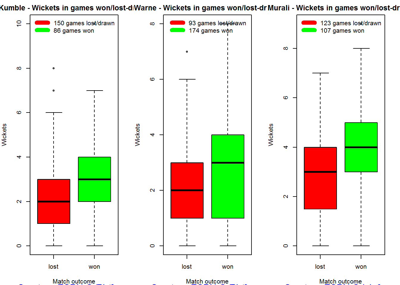
## 15 400 600 229 187 208 186Contribution to matches won and lost
par(mfrow=c(2,2))
par(mar=c(4,4,2,2))
batsmanContributionWonLost(35320,"Tendulkar")
batsmanContributionWonLost(28114,"Dravid")
batsmanContributionWonLost(28779,"Ganguly")
batsmanContributionWonLost(28794,"Gavaskar")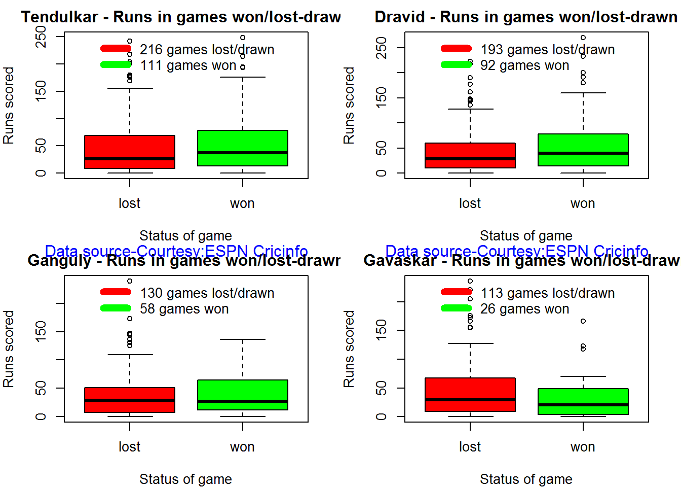
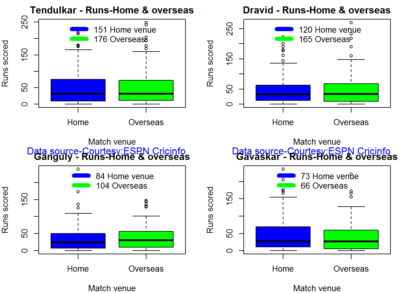
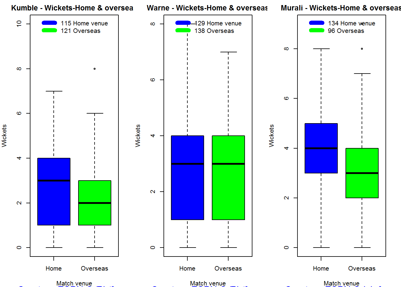
Home and overseas performance
From the plot below Tendulkar and Dravid have a lot more matches both home and abroad and their performance has good both at home and overseas. Tendulkar has the best performance home and abroad and is consistent all across. Dravid is also cossistent at all venues. Gavaskar played fewer matches than Tendulkar & Dravid. The range of runs at home is higher than overseas, however the average is consistent both at home and abroad. Finally we have Ganguly.
par(mfrow=c(2,2))
par(mar=c(4,4,2,2))
batsmanPerfHomeAway(35320,"Tendulkar")
batsmanPerfHomeAway(28114,"Dravid")
batsmanPerfHomeAway(28779,"Ganguly")
batsmanPerfHomeAway(28794,"Gavaskar")

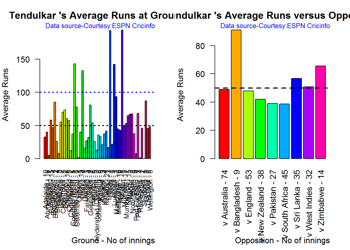
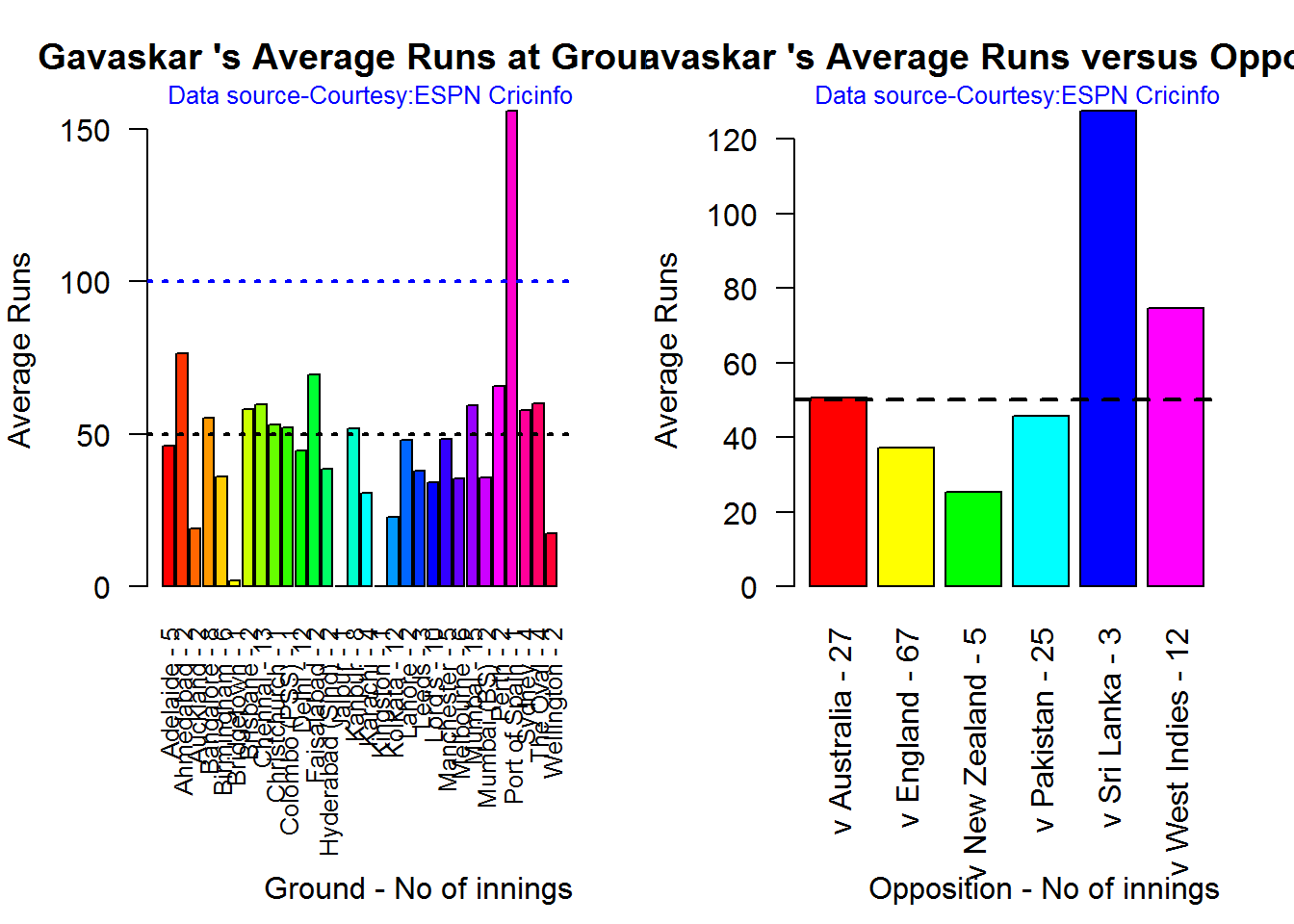
Average runs at ground and against opposition
Tendulkar has above 50 runs average against Sri Lanka, Bangladesh, West Indies and Zimbabwe. The performance against Australia and England average very close to 50. Sydney, Port Elizabeth, Bloemfontein, Collombo are great huntings grounds for Tendulkar
par(mfrow=c(1,2))
par(mar=c(4,4,2,2))
batsmanAvgRunsGround("./tendulkar.csv","Tendulkar")
batsmanAvgRunsOpposition("./tendulkar.csv","Tendulkar")

dev.off()## null device
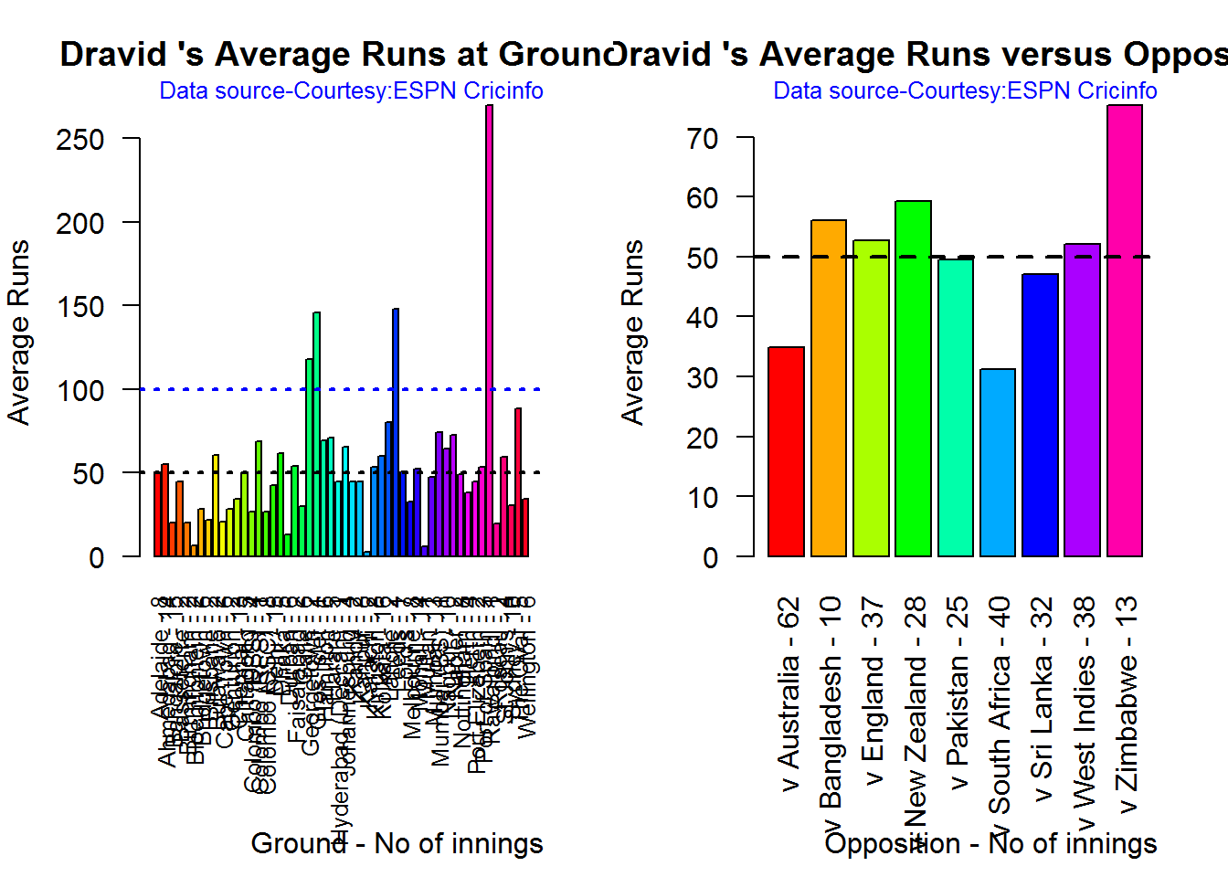
## 1Dravid plundered runs at Adelaide, Georgetown, Oval, Hamiltom etc. Dravid has above average against England, Bangaldesh, New Zealand, Pakistan, West Indies and Zimbabwe
par(mfrow=c(1,2))
par(mar=c(4,4,2,2))
batsmanAvgRunsGround("./dravid.csv","Dravid")
batsmanAvgRunsOpposition("./dravid.csv","Dravid")

dev.off()## null device
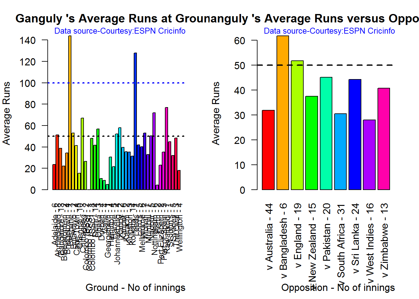
## 1Ganguly has good performance at the Oval, Rawalpindi, Johannesburg and Kandy. Ganguly averages 50 runs against England and Bangladesh.
par(mfrow=c(1,2))
par(mar=c(4,4,2,2))
batsmanAvgRunsGround("./ganguly.csv","Ganguly")
batsmanAvgRunsOpposition("./ganguly.csv","Ganguly")

dev.off()## null device
## 1The Oval, Sydney, Perth, Melbourne, Brisbane, Manchester are happy hunting grounds for Gavaskar. Gavaskar averages around 50 runs Australia, Pakistan, Sri Lanka, West Indies.
par(mfrow=c(1,2))
par(mar=c(4,4,2,2))
batsmanAvgRunsGround("./gavaskar.csv","Gavaskar")
batsmanAvgRunsOpposition("./gavaskar.csv","Gavaskar")

dev.off()## null device
## 1Key findings
Here are some key conclusions
- Tendulkar has the highest average among the 4. He is followed by Dravid, Gavaskar and Ganguly.
- Tendulkar’s predicted performance for a given number of Balls Faced and Minutes at Crease is superior to the rest
- Dravid averages above 50 against 6 countries
- West Indies and Australia are Gavaskar’s favorite batting grounds
- Ganguly has a very good Mean Strike Rate for the range 40-80 and Tendulkar from 100-180
- In home and overseas performance, Tendulkar is the best. Dravid and Gavaskar also have good performance overseas.
- Dravid and Gavaskar probably retired a year or two earlier while Tendulkar and Ganguly’s time was clearly up
Final thoughts
Tendulkar is clearly the greatest batsman India has produced as he leads in almost all aspects of batting – number of centuries, strike rate, predicted runs and home and overseas performance. Dravid follows Tendulkar with 48 centuries, consistent performance home and overseas and a career that was still green. Gavaskar has fewer matches than rest but his performance overseas is very good in those helmetless times. Finally we have Ganguly.
Dravid and Gavaskar had a few more years of great batting while Tendulkar and Ganguly’s career was on a decline.
Note:It is really not fair to include Gavaskar in the analysis as he played in a different era when helmets were not used, even against the fiery pace of Thomson, Lillee, Roberts, Holding etc. In addition Gavaskar did not play against some of the newer countries like Bangladesh and Zimbabwe where he could have amassed runs. Yet I wanted to include him and his performance is clearly excellent
Also see my other posts in R
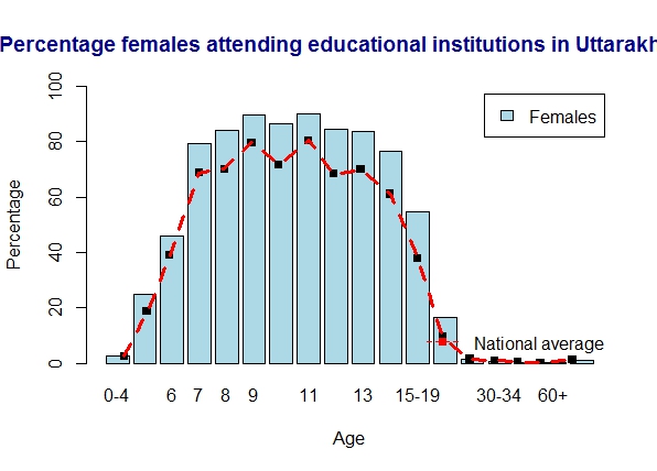
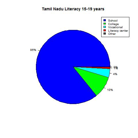
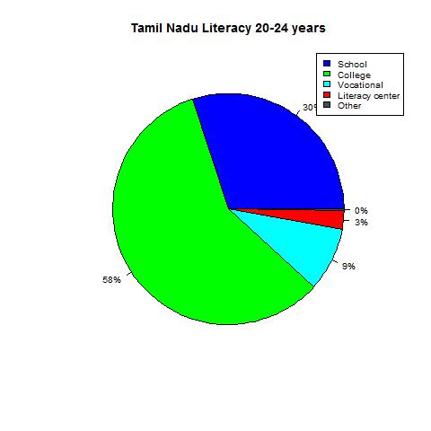
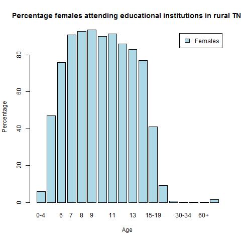
- A peek into literacy in India: Statistical Learning with R
- A crime map of India in R – Crimes against women
- Analyzing cricket’s batting legends – Through the mirage with R
- Masters of Spin: Unraveling the web with R
- Mirror, mirror . the best batsman of them all?
You may also like
- A crime map of India in R: Crimes against women
- What’s up Watson? Using IBM Watson’s QAAPI with Bluemix, NodeExpress – Part 1
- Bend it like Bluemix, MongoDB with autoscaling – Part 2
- Informed choices through Machine Learning : Analyzing Kohli, Tendulkar and Dravid
- Thinking Web Scale (TWS-3): Map-Reduce – Bring compute to data
- Deblurring with OpenCV:Weiner filter reloaded


 Checkout my book ‘Deep Learning from first principles Second Edition- In vectorized Python, R and Octave’. My book is available on Amazon as


