1. Introduction

You don’t understand anything until you learn it more than one way. Marvin Minsky
No computer has ever been designed that is ever aware of what it’s doing; but most of the time, we aren’t either. Marvin Minsky
A wealth of information creates a poverty of attention. Herbert Simon

This post, Deep Learning from first Principles in Python, R and Octave-Part8, is my final post in my Deep Learning from first principles series. In this post, I discuss and implement a key functionality needed while building Deep Learning networks viz. ‘Gradient Checking’. Gradient Checking is an important method to check the correctness of your implementation, specifically the forward propagation and the backward propagation cycles of an implementation. In addition I also discuss some tips for tuning hyper-parameters of a Deep Learning network based on my experience.

My post in this  ‘Deep Learning Series’ so far were
1. Deep Learning from first principles in Python, R and Octave – Part 1 In part 1, I implement logistic regression as a neural network in vectorized Python, R and Octave
2. Deep Learning from first principles in Python, R and Octave – Part 2 In the second part I implement a simple Neural network with just 1 hidden layer and a sigmoid activation output function
3. Deep Learning from first principles in Python, R and Octave – Part 3 The 3rd part implemented a multi-layer Deep Learning Network with sigmoid activation output in vectorized Python, R and Octave
4. Deep Learning from first principles in Python, R and Octave – Part 4 The 4th part deals with multi-class classification. Specifically, I derive the Jacobian of the Softmax function and enhance my L-Layer DL network to include Softmax output function in addition to Sigmoid activation
5. Deep Learning from first principles in Python, R and Octave – Part 5 This post uses the Softmax classifier implemented to classify MNIST digits using a L-layer Deep Learning network
6. Deep Learning from first principles in Python, R and Octave – Part 6 The 6th part adds more bells and whistles to my L-Layer DL network, by including different initialization types namely He and Xavier. Besides L2 Regularization and random dropout is added.
7. Deep Learning from first principles in Python, R and Octave – Part 7 The 7th part deals with Stochastic Gradient Descent Optimization methods including momentum, RMSProp and Adam
8. Deep Learning from first principles in Python, R and Octave – Part 8 – This post implements a critical function for ensuring the correctness of a L-Layer Deep Learning network implementation using Gradient Checking

Checkout my book ‘Deep Learning from first principles: Second Edition – In vectorized Python, R and Octave’. My book starts with the implementation of a simple 2-layer Neural Network and works its way to a generic L-Layer Deep Learning Network, with all the bells and whistles. The derivations have been discussed in detail. The code has been extensively commented and included in its entirety in the Appendix sections. My book is available on Amazon as paperback ($18.99) and in kindle version($9.99/Rs449).

You may also like my companion book “Practical Machine Learning with R and Python- Machine Learning in stereo” available in Amazon in paperback($9.99) and Kindle($6.99) versions. This book is ideal for a quick reference of the various ML functions and associated measurements in both R and Python which are essential to delve deep into Deep Learning.

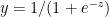
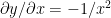
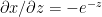
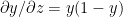
Gradient Checking is based on the following approach. One iteration of Gradient Descent computes and updates the parameters by doing
.
To minimize the cost we will need to minimize
Let be a function that computes the derivative . Gradient Checking allows us to numerically evaluate the implementation of the function and verify its correctness.
We know the derivative of a function is given by

Note: The above derivative is based on the 2 sided derivative. The 1-sided derivative  is given by
Gradient Checking is based on the 2-sided derivative because the error is of the order as opposed for the 1-sided derivative.
Hence Gradient Check uses the 2 sided derivative as follows.

In Gradient Check the following is done
A) Run one normal cycle of your implementation by doing the following
a) Compute the output activation by running 1 cycle of forward propagation
b) Compute the cost using the output activation
c) Compute the gradients using backpropation (grad)

B) Perform gradient check steps as below
a) Set . Flatten all ‘weights’ and ‘bias’ matrices and vectors to a column vector.
b) Initialize by bumping up by adding ()
c) Perform forward propagation with
d) Compute cost with i.e.
e) Initialize  by bumping down by subtracting
f) Perform forward propagation with
g) Compute cost with i.e. 
h) Compute or ‘gradapprox’ asusing the 2 sided derivative.
i) Compute L2norm or the Euclidean distance between ‘grad’ and ‘gradapprox’. If the
diference is of the order of or the implementation is correct. In the Deep Learning Specialization Prof Andrew Ng mentions that if the difference is of the order of then the implementation is correct. A difference of is also ok. Anything more than that is a cause of worry and you should look at your code more closely. To see more details click Gradient checking and advanced optimization

You can clone/download the code from Github at DeepLearning-Part8

After spending a better part of 3 days, I now realize how critical Gradient Check is for ensuring the correctness of you implementation. Initially I was getting very high difference and did not know how to understand the results or debug my implementation. After many hours of staring at the results, I  was able to finally arrive at a way, to localize issues in the implementation. In fact, I did catch a small bug in my Python code, which did not exist in the R and Octave implementations. I will demonstrate this below

1.1a Gradient Check – Sigmoid Activation – Python

import numpy as np
import matplotlib

exec(open("DLfunctions8.py").read())
exec(open("testcases.py").read())
#Load the data
train_X, train_Y, test_X, test_Y = load_dataset()
#Set layer dimensions
layersDimensions = [2,4,1]  
parameters = initializeDeepModel(layersDimensions)
#Perform forward prop
AL, caches, dropoutMat = forwardPropagationDeep(train_X, parameters, keep_prob=1, hiddenActivationFunc="relu",outputActivationFunc="sigmoid")
#Compute cost
cost = computeCost(AL, train_Y, outputActivationFunc="sigmoid") 
print("cost=",cost)
#Perform backprop and get gradients
gradients = backwardPropagationDeep(AL, train_Y, caches, dropoutMat, lambd=0, keep_prob=1,                                   hiddenActivationFunc="relu",outputActivationFunc="sigmoid")

epsilon = 1e-7
outputActivationFunc="sigmoid"

# Set-up variables
# Flatten parameters to a vector
parameters_values, _ = dictionary_to_vector(parameters)
#Flatten gradients to a vector
grad = gradients_to_vector(parameters,gradients)
num_parameters = parameters_values.shape[0]
#Initialize
J_plus = np.zeros((num_parameters, 1))
J_minus = np.zeros((num_parameters, 1))
gradapprox = np.zeros((num_parameters, 1))

# Compute gradapprox using 2 sided derivative
for i in range(num_parameters):
    # Compute J_plus[i]. 
    thetaplus = np.copy(parameters_values)                                   
    thetaplus[i][0] = thetaplus[i][0] + epsilon                                 
    AL, caches, dropoutMat = forwardPropagationDeep(train_X, vector_to_dictionary(parameters,thetaplus), keep_prob=1, 
                                              hiddenActivationFunc="relu",outputActivationFunc=outputActivationFunc)
    J_plus[i] = computeCost(AL, train_Y, outputActivationFunc=outputActivationFunc) 
    
    
    # Compute J_minus[i]. 
    thetaminus = np.copy(parameters_values)                                     
    thetaminus[i][0] = thetaminus[i][0] - epsilon                                     
    AL, caches, dropoutMat  = forwardPropagationDeep(train_X, vector_to_dictionary(parameters,thetaminus), keep_prob=1, 
                                              hiddenActivationFunc="relu",outputActivationFunc=outputActivationFunc)     
    J_minus[i] = computeCost(AL, train_Y, outputActivationFunc=outputActivationFunc)                            
       
    # Compute gradapprox[i]   
    gradapprox[i] = (J_plus[i] - J_minus[i])/(2*epsilon)

# Compare gradapprox to backward propagation gradients by computing difference. 
numerator = np.linalg.norm(grad-gradapprox)                                           
denominator = np.linalg.norm(grad) +  np.linalg.norm(gradapprox)                                         
difference =  numerator/denominator                                        

#Check the difference
if difference > 1e-5:
    print ("\033[93m" + "There is a mistake in the backward propagation! difference = " + str(difference) + "\033[0m")
else:
    print ("\033[92m" + "Your backward propagation works perfectly fine! difference = " + str(difference) + "\033[0m")
print(difference)
print("\n")    
# The technique below can be used to identify 
# which of the parameters are in error
# Covert grad to dictionary
m=vector_to_dictionary2(parameters,grad)
print("Gradients from backprop")
print(m)
print("\n")
# Convert gradapprox to dictionary
n=vector_to_dictionary2(parameters,gradapprox)
print("Gradapprox from gradient check")
print(n)

## (300, 2)
## (300,)
## cost= 0.6931455556341791
## [92mYour backward propagation works perfectly fine! difference = 1.1604150683743381e-06[0m
## 1.1604150683743381e-06
## 
## 
## Gradients from backprop
## {'dW1': array([[-6.19439955e-06, -2.06438046e-06],
##        [-1.50165447e-05,  7.50401672e-05],
##        [ 1.33435433e-04,  1.74112143e-04],
##        [-3.40909024e-05, -1.38363681e-04]]), 'db1': array([[ 7.31333221e-07],
##        [ 7.98425950e-06],
##        [ 8.15002817e-08],
##        [-5.69821155e-08]]), 'dW2': array([[2.73416304e-04, 2.96061451e-04, 7.51837363e-05, 1.01257729e-04]]), 'db2': array([[-7.22232235e-06]])}
## 
## 
## Gradapprox from gradient check
## {'dW1': array([[-6.19448937e-06, -2.06501483e-06],
##        [-1.50168766e-05,  7.50399742e-05],
##        [ 1.33435485e-04,  1.74112391e-04],
##        [-3.40910633e-05, -1.38363765e-04]]), 'db1': array([[ 7.31081862e-07],
##        [ 7.98472399e-06],
##        [ 8.16013923e-08],
##        [-5.71764858e-08]]), 'dW2': array([[2.73416290e-04, 2.96061509e-04, 7.51831930e-05, 1.01257891e-04]]), 'db2': array([[-7.22255589e-06]])}

1.1b Gradient Check – Softmax Activation – Python (Error!!)

In the code below I show, how I managed to spot a bug in your implementation

import numpy as np
exec(open("DLfunctions8.py").read())
N = 100 # number of points per class
D = 2 # dimensionality
K = 3 # number of classes
X = np.zeros((N*K,D)) # data matrix (each row = single example)
y = np.zeros(N*K, dtype='uint8') # class labels
for j in range(K):
  ix = range(N*j,N*(j+1))
  r = np.linspace(0.0,1,N) # radius
  t = np.linspace(j*4,(j+1)*4,N) + np.random.randn(N)*0.2 # theta
  X[ix] = np.c_[r*np.sin(t), r*np.cos(t)]
  y[ix] = j


# Plot the data
#plt.scatter(X[:, 0], X[:, 1], c=y, s=40, cmap=plt.cm.Spectral)
layersDimensions = [2,3,3]
y1=y.reshape(-1,1).T
train_X=X.T
train_Y=y1

parameters = initializeDeepModel(layersDimensions)
#Compute forward prop
AL, caches, dropoutMat = forwardPropagationDeep(train_X, parameters, keep_prob=1, 
                                                hiddenActivationFunc="relu",outputActivationFunc="softmax")
#Compute cost
cost = computeCost(AL, train_Y, outputActivationFunc="softmax") 
print("cost=",cost)
#Compute gradients from backprop
gradients = backwardPropagationDeep(AL, train_Y, caches, dropoutMat, lambd=0, keep_prob=1, 
                                    hiddenActivationFunc="relu",outputActivationFunc="softmax")
# Note the transpose of the gradients for Softmax has to be taken
L= len(parameters)//2
print(L)
gradients['dW'+str(L)]=gradients['dW'+str(L)].T
gradients['db'+str(L)]=gradients['db'+str(L)].T
# Perform gradient check
gradient_check_n(parameters, gradients, train_X, train_Y, epsilon = 1e-7,outputActivationFunc="softmax")

cost= 1.0986187818144022
2
There is a mistake in the backward propagation! difference = 0.7100295155692544
0.7100295155692544


Gradients from backprop
{'dW1': array([[ 0.00050125,  0.00045194],
       [ 0.00096392,  0.00039641],
       [-0.00014276, -0.00045639]]), 'db1': array([[ 0.00070082],
       [-0.00224399],
       [ 0.00052305]]), 'dW2': array([[-8.40953794e-05, -9.52657769e-04, -1.10269379e-04],
       [-7.45469382e-04,  9.49795606e-04,  2.29045434e-04],
       [ 8.29564761e-04,  2.86216305e-06, -1.18776055e-04]]), 
     'db2': array([[-0.00253808],
       [-0.00505508],
       [ 0.00759315]])}


Gradapprox from gradient check
{'dW1': array([[ 0.00050125,  0.00045194],
       [ 0.00096392,  0.00039641],
       [-0.00014276, -0.00045639]]), 'db1': array([[ 0.00070082],
       [-0.00224399],
       [ 0.00052305]]), 'dW2': array([[-8.40960634e-05, -9.52657953e-04, -1.10268461e-04],
       [-7.45469242e-04,  9.49796908e-04,  2.29045671e-04],
       [ 8.29565305e-04,  2.86104473e-06, -1.18776100e-04]]), 
     'db2': array([[-8.46211989e-06],
       [-1.68487446e-05],
       [ 2.53108645e-05]])}

Gradient Check gives a high value of the difference of 0.7100295. Inspecting the Gradients and Gradapprox we can see there is a very big discrepancy in db2. After I went over my code I discovered that I my computation in the function layerActivationBackward for Softmax was

 
   # Erroneous code
   if activationFunc == 'softmax':
        dW = 1/numtraining * np.dot(A_prev,dZ)
        db = np.sum(dZ, axis=0, keepdims=True)
        dA_prev = np.dot(dZ,W)
instead of
   # Fixed code
   if activationFunc == 'softmax':
        dW = 1/numtraining * np.dot(A_prev,dZ)
        db = 1/numtraining *  np.sum(dZ, axis=0, keepdims=True)
        dA_prev = np.dot(dZ,W)

After fixing this error when I ran Gradient Check I get

1.1c Gradient Check – Softmax Activation – Python (Corrected!!)

import numpy as np
exec(open("DLfunctions8.py").read())
N = 100 # number of points per class
D = 2 # dimensionality
K = 3 # number of classes
X = np.zeros((N*K,D)) # data matrix (each row = single example)
y = np.zeros(N*K, dtype='uint8') # class labels
for j in range(K):
  ix = range(N*j,N*(j+1))
  r = np.linspace(0.0,1,N) # radius
  t = np.linspace(j*4,(j+1)*4,N) + np.random.randn(N)*0.2 # theta
  X[ix] = np.c_[r*np.sin(t), r*np.cos(t)]
  y[ix] = j


# Plot the data
#plt.scatter(X[:, 0], X[:, 1], c=y, s=40, cmap=plt.cm.Spectral)
layersDimensions = [2,3,3]
y1=y.reshape(-1,1).T
train_X=X.T
train_Y=y1
#Set layer dimensions
parameters = initializeDeepModel(layersDimensions)
#Perform forward prop
AL, caches, dropoutMat = forwardPropagationDeep(train_X, parameters, keep_prob=1, 
                                                hiddenActivationFunc="relu",outputActivationFunc="softmax")
#Compute cost
cost = computeCost(AL, train_Y, outputActivationFunc="softmax") 
print("cost=",cost)
#Compute gradients from backprop
gradients = backwardPropagationDeep(AL, train_Y, caches, dropoutMat, lambd=0, keep_prob=1, 
                                    hiddenActivationFunc="relu",outputActivationFunc="softmax")
# Note the transpose of the gradients for Softmax has to be taken
L= len(parameters)//2
print(L)
gradients['dW'+str(L)]=gradients['dW'+str(L)].T
gradients['db'+str(L)]=gradients['db'+str(L)].T
#Perform gradient check
gradient_check_n(parameters, gradients, train_X, train_Y, epsilon = 1e-7,outputActivationFunc="softmax")

## cost= 1.0986193170234435
## 2
## [92mYour backward propagation works perfectly fine! difference = 5.268804859613151e-07[0m
## 5.268804859613151e-07
## 
## 
## Gradients from backprop
## {'dW1': array([[ 0.00053206,  0.00038987],
##        [ 0.00093941,  0.00038077],
##        [-0.00012177, -0.0004692 ]]), 'db1': array([[ 0.00072662],
##        [-0.00210198],
##        [ 0.00046741]]), 'dW2': array([[-7.83441270e-05, -9.70179498e-04, -1.08715815e-04],
##        [-7.70175008e-04,  9.54478237e-04,  2.27690198e-04],
##        [ 8.48519135e-04,  1.57012608e-05, -1.18974383e-04]]), 'db2': array([[-8.52190476e-06],
##        [-1.69954294e-05],
##        [ 2.55173342e-05]])}
## 
## 
## Gradapprox from gradient check
## {'dW1': array([[ 0.00053206,  0.00038987],
##        [ 0.00093941,  0.00038077],
##        [-0.00012177, -0.0004692 ]]), 'db1': array([[ 0.00072662],
##        [-0.00210198],
##        [ 0.00046741]]), 'dW2': array([[-7.83439980e-05, -9.70180603e-04, -1.08716369e-04],
##        [-7.70173925e-04,  9.54478718e-04,  2.27690089e-04],
##        [ 8.48520143e-04,  1.57018842e-05, -1.18973720e-04]]), 'db2': array([[-8.52096171e-06],
##        [-1.69964043e-05],
##        [ 2.55162558e-05]])}

1.2a Gradient Check – Sigmoid Activation – R

source("DLfunctions8.R")
z <- as.matrix(read.csv("circles.csv",header=FALSE)) 

x <- z[,1:2]
y <- z[,3]
X <- t(x)
Y <- t(y)
#Set layer dimensions
layersDimensions = c(2,5,1)
parameters = initializeDeepModel(layersDimensions)
#Perform forward prop
retvals = forwardPropagationDeep(X, parameters,keep_prob=1, hiddenActivationFunc="relu",
                                 outputActivationFunc="sigmoid")
AL <- retvals[['AL']]
caches <- retvals[['caches']]
dropoutMat <- retvals[['dropoutMat']]
#Compute cost
cost <- computeCost(AL, Y,outputActivationFunc="sigmoid",
                    numClasses=layersDimensions[length(layersDimensions)])
print(cost)

## [1] 0.6931447

# Backward propagation.
gradients = backwardPropagationDeep(AL, Y, caches, dropoutMat, lambd=0, keep_prob=1, hiddenActivationFunc="relu",
                                    outputActivationFunc="sigmoid",numClasses=layersDimensions[length(layersDimensions)])

epsilon = 1e-07
outputActivationFunc="sigmoid"
#Convert parameter list to vector
parameters_values = list_to_vector(parameters)
#Convert gradient list to vector
grad = gradients_to_vector(parameters,gradients)
num_parameters = dim(parameters_values)[1]
#Initialize
J_plus = matrix(rep(0,num_parameters),
                nrow=num_parameters,ncol=1)
J_minus = matrix(rep(0,num_parameters),
                 nrow=num_parameters,ncol=1)
gradapprox = matrix(rep(0,num_parameters),
                    nrow=num_parameters,ncol=1)

# Compute gradapprox
for(i in 1:num_parameters){
    # Compute J_plus[i]. 
    thetaplus = parameters_values                                   
    thetaplus[i][1] = thetaplus[i][1] + epsilon                                 
    retvals = forwardPropagationDeep(X, vector_to_list(parameters,thetaplus), keep_prob=1, 
                                                hiddenActivationFunc="relu",outputActivationFunc=outputActivationFunc)
    
    AL <- retvals[['AL']]
    J_plus[i] = computeCost(AL, Y, outputActivationFunc=outputActivationFunc) 


   # Compute J_minus[i]. 
    thetaminus = parameters_values                                     
    thetaminus[i][1] = thetaminus[i][1] - epsilon                                     
    retvals  = forwardPropagationDeep(X, vector_to_list(parameters,thetaminus), keep_prob=1, 
                                                 hiddenActivationFunc="relu",outputActivationFunc=outputActivationFunc)     
    AL <- retvals[['AL']]
    J_minus[i] = computeCost(AL, Y, outputActivationFunc=outputActivationFunc)                            

    # Compute gradapprox[i]   
    gradapprox[i] = (J_plus[i] - J_minus[i])/(2*epsilon)
}
# Compare gradapprox to backward propagation gradients by computing difference.
#Compute L2Norm
numerator = L2NormVec(grad-gradapprox)                                           
denominator = L2NormVec(grad) +  L2NormVec(gradapprox)                                         
difference =  numerator/denominator 
if(difference > 1e-5){
    cat("There is a mistake, the difference is too high",difference)
} else{
    cat("The implementations works perfectly", difference)
}

## The implementations works perfectly 1.279911e-06

# This can be used to check
print("Gradients from backprop")

## [1] "Gradients from backprop"

vector_to_list2(parameters,grad)

## $dW1
##               [,1]          [,2]
## [1,] -7.641588e-05 -3.427989e-07
## [2,] -9.049683e-06  6.906304e-05
## [3,]  3.401039e-06 -1.503914e-04
## [4,]  1.535226e-04 -1.686402e-04
## [5,] -6.029292e-05 -2.715648e-04
## 
## $db1
##               [,1]
## [1,]  6.930318e-06
## [2,] -3.283117e-05
## [3,]  1.310647e-05
## [4,] -3.454308e-05
## [5,] -2.331729e-08
## 
## $dW2
##              [,1]         [,2]         [,3]        [,4]         [,5]
## [1,] 0.0001612356 0.0001113475 0.0002435824 0.000362149 2.874116e-05
## 
## $db2
##              [,1]
## [1,] -1.16364e-05

print("Grad approx from gradient check")

## [1] "Grad approx from gradient check"

vector_to_list2(parameters,gradapprox)

## $dW1
##               [,1]          [,2]
## [1,] -7.641554e-05 -3.430589e-07
## [2,] -9.049428e-06  6.906253e-05
## [3,]  3.401168e-06 -1.503919e-04
## [4,]  1.535228e-04 -1.686401e-04
## [5,] -6.029288e-05 -2.715650e-04
## 
## $db1
##               [,1]
## [1,]  6.930012e-06
## [2,] -3.283096e-05
## [3,]  1.310618e-05
## [4,] -3.454237e-05
## [5,] -2.275957e-08
## 
## $dW2
##              [,1]         [,2]         [,3]         [,4]        [,5]
## [1,] 0.0001612355 0.0001113476 0.0002435829 0.0003621486 2.87409e-05
## 
## $db2
##              [,1]
## [1,] -1.16368e-05

1.2b Gradient Check – Softmax Activation – R

source("DLfunctions8.R")
Z <- as.matrix(read.csv("spiral.csv",header=FALSE)) 

# Setup the data
X <- Z[,1:2]
y <- Z[,3]
X <- t(X)
Y <- t(y)
layersDimensions = c(2, 3, 3)
parameters = initializeDeepModel(layersDimensions)
#Perform forward prop
retvals = forwardPropagationDeep(X, parameters,keep_prob=1, hiddenActivationFunc="relu",
                                 outputActivationFunc="softmax")
AL <- retvals[['AL']]
caches <- retvals[['caches']]
dropoutMat <- retvals[['dropoutMat']]
#Compute cost
cost <- computeCost(AL, Y,outputActivationFunc="softmax",
                    numClasses=layersDimensions[length(layersDimensions)])
print(cost)

## [1] 1.098618

# Backward propagation.
gradients = backwardPropagationDeep(AL, Y, caches, dropoutMat, lambd=0, keep_prob=1, hiddenActivationFunc="relu",
                                    outputActivationFunc="softmax",numClasses=layersDimensions[length(layersDimensions)])

# Need to take transpose of the last layer for Softmax
L=length(parameters)/2
gradients[[paste('dW',L,sep="")]]=t(gradients[[paste('dW',L,sep="")]])
gradients[[paste('db',L,sep="")]]=t(gradients[[paste('db',L,sep="")]])
#Perform gradient check
gradient_check_n(parameters, gradients, X, Y, 
                 epsilon = 1e-7,outputActivationFunc="softmax")

## The implementations works perfectly 3.903011e-07[1] "Gradients from backprop"
## $dW1
##              [,1]          [,2]
## [1,] 0.0007962367 -0.0001907606
## [2,] 0.0004444254  0.0010354412
## [3,] 0.0003078611  0.0007591255
## 
## $db1
##               [,1]
## [1,] -0.0017305136
## [2,]  0.0005393734
## [3,]  0.0012484550
## 
## $dW2
##               [,1]          [,2]          [,3]
## [1,] -3.515627e-04  7.487283e-04 -3.971656e-04
## [2,] -6.381521e-05 -1.257328e-06  6.507254e-05
## [3,] -1.719479e-04 -4.857264e-04  6.576743e-04
## 
## $db2
##               [,1]
## [1,] -5.536383e-06
## [2,] -1.824656e-05
## [3,]  2.378295e-05
## 
## [1] "Grad approx from gradient check"
## $dW1
##              [,1]          [,2]
## [1,] 0.0007962364 -0.0001907607
## [2,] 0.0004444256  0.0010354406
## [3,] 0.0003078615  0.0007591250
## 
## $db1
##               [,1]
## [1,] -0.0017305135
## [2,]  0.0005393741
## [3,]  0.0012484547
## 
## $dW2
##               [,1]          [,2]          [,3]
## [1,] -3.515632e-04  7.487277e-04 -3.971656e-04
## [2,] -6.381451e-05 -1.257883e-06  6.507239e-05
## [3,] -1.719469e-04 -4.857270e-04  6.576739e-04
## 
## $db2
##               [,1]
## [1,] -5.536682e-06
## [2,] -1.824652e-05
## [3,]  2.378209e-05

1.3a Gradient Check – Sigmoid Activation – Octave

source("DL8functions.m")
################## Circles
data=csvread("circles.csv");

X=data(:,1:2);
Y=data(:,3);
#Set layer dimensions
layersDimensions = [2 5  1]; #tanh=-0.5(ok), #relu=0.1 best!
[weights biases] = initializeDeepModel(layersDimensions);
#Perform forward prop
[AL forward_caches activation_caches droputMat] = forwardPropagationDeep(X', weights, biases,keep_prob=1, 
                 hiddenActivationFunc="relu", outputActivationFunc="sigmoid");
#Compute cost
cost = computeCost(AL, Y',outputActivationFunc=outputActivationFunc,numClasses=layersDimensions(size(layersDimensions)(2)));
disp(cost);
#Compute gradients from cost
[gradsDA gradsDW gradsDB] = backwardPropagationDeep(AL, Y', activation_caches,forward_caches, droputMat, lambd=0, keep_prob=1, 
                                 hiddenActivationFunc="relu", outputActivationFunc="sigmoid",
                                 numClasses=layersDimensions(size(layersDimensions)(2)));
epsilon = 1e-07;
outputActivationFunc="sigmoid";
# Convert paramter cell array to vector
parameters_values = cellArray_to_vector(weights, biases);
#Convert gradient cell array to vector
grad = gradients_to_vector(gradsDW,gradsDB);
num_parameters = size(parameters_values)(1);
#Initialize
J_plus = zeros(num_parameters, 1);
J_minus = zeros(num_parameters, 1);
gradapprox = zeros(num_parameters, 1);
# Compute gradapprox
for i = 1:num_parameters
    # Compute J_plus[i]. 
    thetaplus = parameters_values;                                   
    thetaplus(i,1) = thetaplus(i,1) + epsilon;      
    [weights1 biases1] =vector_to_cellArray(weights, biases,thetaplus);    
    [AL forward_caches activation_caches droputMat] = forwardPropagationDeep(X', weights1, biases1, keep_prob=1, 
                                              hiddenActivationFunc="relu",outputActivationFunc=outputActivationFunc);
    J_plus(i) = computeCost(AL, Y', outputActivationFunc=outputActivationFunc); 
        
    # Compute J_minus[i]. 
    thetaminus = parameters_values;                                  
    thetaminus(i,1) = thetaminus(i,1) - epsilon ;    
    [weights1 biases1] = vector_to_cellArray(weights, biases,thetaminus);    
    [AL forward_caches activation_caches droputMat]  = forwardPropagationDeep(X',weights1, biases1, keep_prob=1, 
                                              hiddenActivationFunc="relu",outputActivationFunc=outputActivationFunc);     
    J_minus(i) = computeCost(AL, Y', outputActivationFunc=outputActivationFunc);                            
      
    # Compute gradapprox[i]   
    gradapprox(i) = (J_plus(i) - J_minus(i))/(2*epsilon);

endfor

#Compute L2Norm
numerator = L2NormVec(grad-gradapprox);                                           
denominator = L2NormVec(grad) +  L2NormVec(gradapprox);                                         
difference =  numerator/denominator;
disp(difference);
#Check difference
if difference > 1e-04
   printf("There is a mistake in the implementation ");
   disp(difference);
else
   printf("The implementation works perfectly");
      disp(difference);
endif
[weights1 biases1] = vector_to_cellArray(weights, biases,grad);  
printf("Gradients from back propagation"); 
disp(weights1);
disp(biases1); 
[weights2 biases2] = vector_to_cellArray(weights, biases,gradapprox); 
printf("Gradients from gradient check");
disp(weights2);
disp(biases2); 

0.69315
1.4893e-005
The implementation works perfectly 1.4893e-005
Gradients from back propagation
{
[1,1] =
5.0349e-005 2.1323e-005
8.8632e-007 1.8231e-006
9.3784e-005 1.0057e-004
1.0875e-004 -1.9529e-007
5.4502e-005 3.2721e-005
[1,2] =
1.0567e-005 6.0615e-005 4.6004e-005 1.3977e-004 1.0405e-004
}
{
[1,1] =
-1.8716e-005
1.1309e-009
4.7686e-005
1.2051e-005
-1.4612e-005
[1,2] = 9.5808e-006
}
Gradients from gradient check
{
[1,1] =
5.0348e-005 2.1320e-005
8.8485e-007 1.8219e-006
9.3784e-005 1.0057e-004
1.0875e-004 -1.9762e-007
5.4502e-005 3.2723e-005
[1,2] =
[1,2] =
1.0565e-005 6.0614e-005 4.6007e-005 1.3977e-004 1.0405e-004
}
{
[1,1] =
-1.8713e-005
1.1102e-009
4.7687e-005
1.2048e-005
-1.4609e-005
[1,2] = 9.5790e-006
}

1.3b Gradient Check – Softmax Activation – Octave

source("DL8functions.m")
data=csvread("spiral.csv");

# Setup the data
X=data(:,1:2);
Y=data(:,3);
# Set the layer dimensions
layersDimensions = [2 3  3]; 
[weights biases] = initializeDeepModel(layersDimensions);
# Run forward prop
[AL forward_caches activation_caches droputMat] = forwardPropagationDeep(X', weights, biases,keep_prob=1, 
                 hiddenActivationFunc="relu", outputActivationFunc="softmax");
# Compute cost
cost = computeCost(AL, Y',outputActivationFunc=outputActivationFunc,numClasses=layersDimensions(size(layersDimensions)(2)));
disp(cost);
# Perform backward prop
[gradsDA gradsDW gradsDB] = backwardPropagationDeep(AL, Y', activation_caches,forward_caches, droputMat, lambd=0, keep_prob=1, 
                                 hiddenActivationFunc="relu", outputActivationFunc="softmax",
                                 numClasses=layersDimensions(size(layersDimensions)(2)));

#Take transpose of last layer for Softmax                                
L=size(weights)(2);
gradsDW{L}= gradsDW{L}';
gradsDB{L}= gradsDB{L}';   
#Perform gradient check
difference= gradient_check_n(weights, biases, gradsDW,gradsDB, X, Y, epsilon = 1e-7,
                  outputActivationFunc="softmax",numClasses=layersDimensions(size(layersDimensions)(2)));

 1.0986
The implementation works perfectly  2.0021e-005
Gradients from back propagation
{
  [1,1] =
    -7.1590e-005  4.1375e-005
    -1.9494e-004  -5.2014e-005
    -1.4554e-004  5.1699e-005
  [1,2] =
    3.3129e-004  1.9806e-004  -1.5662e-005
    -4.9692e-004  -3.7756e-004  -8.2318e-005
    1.6562e-004  1.7950e-004  9.7980e-005
}
{
  [1,1] =
    -3.0856e-005
    -3.3321e-004
    -3.8197e-004
  [1,2] =
    1.2046e-006
    2.9259e-007
    -1.4972e-006
}
Gradients from gradient check
{
  [1,1] =
    -7.1586e-005  4.1377e-005
    -1.9494e-004  -5.2013e-005
    -1.4554e-004  5.1695e-005
    3.3129e-004  1.9806e-004  -1.5664e-005
    -4.9692e-004  -3.7756e-004  -8.2316e-005
    1.6562e-004  1.7950e-004  9.7979e-005
}
{
  [1,1] =
    -3.0852e-005
    -3.3321e-004
    -3.8197e-004
  [1,2] =
    1.1902e-006
    2.8200e-007
    -1.4644e-006
}

2.1 Tip for tuning hyperparameters

Deep Learning Networks come with a large number of hyper parameters which require tuning. The hyper parameters are

1. -learning rate
2. Number of layers
3. Number of hidden units
4. Number of iterations
5. Momentum – – 0.9
6. RMSProp – – 0.9
7. Adam – , and
8. learning rate decay
9. mini batch size
10. Initialization method – He, Xavier
11. Regularization

– Among the above the most critical is learning rate  . Rather than just trying out random values, it may help to try out values on a logarithmic scale. So we could try out values -0.01,0.1,1.0,10 etc. If we find that the cost is between 0.01 and 0.1 we could use a technique similar to binary search or bisection, so we can try 0.01, 0.05. If we need to be bigger than 0.01 and 0.05 we could try 0.25  and then keep halving the distance etc.
– The performance of Momentum and RMSProp are very good and work well with values 0.9. Even with this, it is better to try out values of 1- in the logarithmic range. So 1- could 0.001,0.01,0.1 and hence would be 0.999,0.99 or 0.9
– Increasing the number of hidden units or number of hidden layers need to be done gradually. I have noticed that increasing number of hidden layers heavily does not improve performance and sometimes degrades it.
– Sometimes, I tend to increase the number of iterations if I think I see a steady decrease in the cost for a certain learning rate
– It may also help to add learning rate decay if you see there is an oscillation while it decreases.
– Xavier and He initializations also help in a fast convergence and are worth trying out.

3.1 Final thoughts

As I come to a close in this Deep Learning Series from first principles in Python, R and Octave, I must admit that I learnt a lot in the process.

* Building a L-layer, vectorized Deep Learning Network in Python, R and Octave was extremely challenging but very rewarding
* One benefit of building vectorized versions in Python, R and Octave was that I was looking at each function that I was implementing thrice, and hence I was able to fix any bugs in any of the languages
* In addition since I built the generic L-Layer DL network with all the bells and whistles, layer by layer I further had an opportunity to look at all the functions in each successive post.
* Each language has its advantages and disadvantages. From the performance perspective I think Python is the best, followed by Octave and then R
* Interesting, I noticed that even if small bugs creep into your implementation, the DL network does learn and does generate a valid set of weights and biases, however this may not be an optimum solution. In one case of an inadvertent bug, I was not updating the weights in the final layer of the DL network. Yet, using all the other layers, the DL network was able to come with a reasonable solution (maybe like random dropout, remaining units can still learn the data!)
* Having said that, the Gradient Check method discussed and implemented in this post can be very useful in ironing out bugs.
Feel free to clone/download the code from Github at DeepLearning-Part8

Conclusion

These last couple of months when I was writing the posts and the also churning up the code in Python, R and Octave were  very hectic. There have been times when I found that implementations of some function to be extremely demanding and I almost felt like giving up. Other times, I have spent quite some time on an intractable DL network which would not respond to changes in hyper-parameters. All in all, it was a great learning experience. I would suggest that you start from my first post Deep Learning from first principles in Python, R and Octave-Part 1 and work your way up. Feel free to take the code apart and try out things. That is the only way you will learn.

Hope you had as much fun as I had. Stay tuned. I will be back!!!

Also see
1. My book ‘Practical Machine Learning with R and Python’ on Amazon
2. Revisiting crimes against women in India
3. Literacy in India – A deepR dive
4. Sixer – R package cricketr’s new Shiny avatar
5. Bend it like Bluemix, MongoDB using Auto-scale – Part 1!
6. Computer Vision: Ramblings on derivatives, histograms and contours
7. Introducing QCSimulator: A 5-qubit quantum computing simulator in R
8. A closer look at “Robot Horse on a Trot” in Android

To see all post click Index of Posts