My presentations on ‘Elements of Neural Networks & Deep Learning’ -Parts 4,5

This is the next set of presentations on “Elements of Neural Networks and Deep Learning”. In the 4th presentation I discuss and derive the generalized equations for a multi-unit, multi-layer Deep Learning network. The 5th presentation derives the equations for a Deep Learning network when performing multi-class classification along with the derivations for cross-entropy loss. The corresponding implementations are available in vectorized R, Python and Octave are available in my book ‘Deep Learning from first principles:Second edition- In vectorized Python, R and Octave‘

Important note: Do check out my later version of these videos at Take 4+: Presentations on ‘Elements of Neural Networks and Deep Learning’ – Parts 1-8 . These have more content and also include some corrections. Check it out!

1. Elements of Neural Network and Deep Learning – Part 4
This presentation is a continuation of my 3rd presentation in which I derived the equations for a simple 3 layer Neural Network with 1 hidden layer. In this video presentation, I discuss step-by-step the derivations for a L-Layer, multi-unit Deep Learning Network, with any activation function g(z)

The implementations of L-Layer, multi-unit Deep Learning Network in vectorized R, Python and Octave are available in my post Deep Learning from first principles in Python, R and Octave – Part 3

2. Elements of Neural Network and Deep Learning – Part 5
This presentation discusses multi-class classification using the Softmax function. The detailed derivation for the Jacobian of the Softmax is discussed, and subsequently the derivative of cross-entropy loss is also discussed in detail. Finally the final set of equations for a Neural Network with multi-class classification is derived.

The corresponding implementations in vectorized R, Python and Octave are available in the following posts
a. Deep Learning from first principles in Python, R and Octave – Part 4
b. Deep Learning from first principles in Python, R and Octave – Part 5

To be continued. Watch this space!

Checkout my book ‘Deep Learning from first principles: Second Edition – In vectorized Python, R and Octave’. My book starts with the implementation of a simple 2-layer Neural Network and works its way to a generic L-Layer Deep Learning Network, with all the bells and whistles. The derivations have been discussed in detail. The code has been extensively commented and included in its entirety in the Appendix sections. My book is available on Amazon as paperback ($18.99) and in kindle version($9.99/Rs449).

Also see
1. My book ‘Practical Machine Learning in R and Python: Third edition’ on Amazon
2. Big Data-2: Move into the big league:Graduate from R to SparkR
3. Introducing QCSimulator: A 5-qubit quantum computing simulator in R
4. My TEDx talk on the “Internet of Things
5. Rock N’ Roll with Bluemix, Cloudant & NodeExpress
6. GooglyPlus: yorkr analyzes IPL players, teams, matches with plots and tables
7. Literacy in India – A deepR dive
8. Fun simulation of a Chain in Android

To see all posts click Index of Posts

My book “Deep Learning from first principles” now on Amazon

Note: The 2nd edition of this book is now available on Amazon

My 4th book(self-published), “Deep Learning from first principles – In vectorized Python, R and Octave” (557 pages), is now available on Amazon in both paperback ($18.99) and kindle ($9.99/Rs449). The book starts with the most primitive 2-layer Neural Network and works its way to a generic L-layer Deep Learning Network, with all the bells and whistles. The book includes detailed derivations and vectorized implementations in Python, R and Octave. The code has been extensively commented and has been included in the Appendix section.

Pick up your copy today!!!

My other books
1. Practical Machine Learning with R and Python
2. Beaten by sheer pace – Cricket analytics with yorkr
3. Cricket analytics with cricketr

Deep Learning from first principles in Python, R and Octave – Part 3

“Once upon a time, I, Chuang Tzu, dreamt I was a butterfly, fluttering hither and thither, to all intents and purposes a butterfly. I was conscious only of following my fancies as a butterfly, and was unconscious of my individuality as a man. Suddenly, I awoke, and there I lay, myself again. Now I do not know whether I was then a man dreaming I was a butterfly, or whether I am now a butterfly dreaming that I am a man.”
from The Brain: The Story of you – David Eagleman

“Thought is a great big vector of neural activity”
Prof Geoffrey Hinton

Introduction

This is the third part in my series on Deep Learning from first principles in Python, R and Octave. In the first part Deep Learning from first principles in Python, R and Octave-Part 1, I implemented logistic regression as a 2 layer neural network. The 2nd part Deep Learning from first principles in Python, R and Octave-Part 2, dealt with the implementation of 3 layer Neural Networks with 1 hidden layer to perform classification tasks, where the 2 classes cannot be separated by a linear boundary. In this third part, I implement a multi-layer, Deep Learning (DL) network of arbitrary depth (any number of hidden layers) and arbitrary height (any number of activation units in each hidden layer). The implementations of these Deep Learning networks, in all the 3 parts, are based on vectorized versions in Python, R and Octave. The implementation in the 3rd part is for a L-layer Deep Netwwork, but without any regularization, early stopping, momentum or learning rate adaptation techniques. However even the barebones multi-layer DL, is a handful and has enough hyperparameters to fine-tune and adjust.

The implementation of the vectorized L-layer Deep Learning network in Python, R and Octave were both exhausting, and exacting!! Keeping track of the indices, layer number and matrix dimensions required quite bit of focus. While the implementation was demanding, it was also very exciting to get the code to work. The trick was to be able to shift gears between the slight quirkiness between the languages. Here are some of challenges I faced.

1. Python and Octave allow multiple return values to be unpacked in a single statement. With R, unpacking multiple return values from a list, requires the list returned, to be unpacked separately. I did see that there is a package gsubfn, which does this. I hope this feature becomes a base R feature.
2. Python and R allow dissimilar elements to be saved and returned from functions using dictionaries or lists respectively. However there is no real equivalent in Octave. The closest I got to this functionality in Octave, was the ‘cell array’. But the cell array can be accessed only by the index, and not with the key as in a Python dictionary or R list. This makes things just a bit more difficult in Octave.
3. Python and Octave include implicit broadcasting. In R, broadcasting is not implicit, but R has a nifty function, the sweep(), with which we can broadcast either by columns or by rows
4. The closest equivalent of Python’s dictionary, or R’s list, in Octave is the cell array. However I had to manage separate cell arrays for weights and biases and during gradient descent and separate gradients dW and dB
5. In Python the rank-1 numpy arrays can be annoying at times. This issue is not present in R and Octave.

Though the number of lines of code for Deep Learning functions in Python, R and Octave are about ~350 apiece, they have been some of the most difficult code I have implemented. The current vectorized implementation supports the relu, sigmoid and tanh activation functions as of now. I will be adding other activation functions like the ‘leaky relu’, ‘softmax’ and others, to the implementation in the weeks to come.

While testing with different hyper-parameters namely i) the number of hidden layers, ii) the number of activation units in each layer, iii) the activation function and iv) the number iterations, I found the L-layer Deep Learning Network to be very sensitive to these hyper-parameters. It is not easy to tune the parameters. Adding more hidden layers, or more units per layer, does not help and mostly results in gradient descent getting stuck in some local minima. It does take a fair amount of trial and error and very close observation on how the DL network performs for logical changes. We then can zero in on the most the optimal solution. Feel free to download/fork my code from Github DeepLearning-Part 3 and play around with the hyper-parameters for your own problems.

Derivation of a Multi Layer Deep Learning Network

Note: A detailed discussion of the derivation below is available in my video presentation Neural Network 4
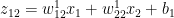
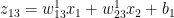
Lets take a simple 3 layer Neural network with 3 hidden layers and an output layer

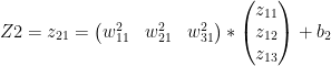
In the forward propagation cycle the equations are

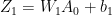
$Z_{1} = W_{1}A_{0} +b_{1}$ and $A_{1} = g(Z_{1})$
$Z_{2} = W_{2}A_{1} +b_{2}$ and $A_{2} = g(Z_{2})$
$Z_{3} = W_{3}A_{2} +b_{3}$ and $A_{3} = g(Z_{3})$

The loss function is given by
$L = -(ylogA3 + (1-y)log(1-A3))$
and $dL/dA3 = -(Y/A_{3} + (1-Y)/(1-A_{3}))$

For a binary classification the output activation function is the sigmoid function given by
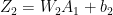
$A_{3} = 1/(1+ e^{-Z3})$ . It can be shown that
$dA_{3}/dZ_{3} = A_{3}(1-A_3)$ see equation 2 in Part 1

$\partial L/\partial Z_{3} = \partial L/\partial A_{3}* \partial A_{3}/\partial Z_{3} = A3-Y$ see equation (f) in Part 1
and since
$\partial L/\partial A_{2} = \partial L/\partial Z_{3} * \partial Z_{3}/\partial A_{2} = (A_{3} -Y) * W_{3}$ because $\partial Z_{3}/\partial A_{2} = W_{3}$ -(1a)
and $\partial L/\partial Z_{2} =\partial L/\partial A_{2} * \partial A_{2}/\partial Z_{2} = (A_{3} -Y) * W_{3} *g'(Z_{2})$ -(1b)
$\partial L/\partial W_{2} = \partial L/\partial Z_{2} * A_{1}$ -(1c)
since $\partial Z_{2}/\partial W_{2} = A_{1}$
and
$\partial L/\partial b_{2} = \partial L/\partial Z_{2}$ -(1d)
because
$\partial Z_{2}/\partial b_{2} =1$

Also

$\partial L/\partial A_{1} =\partial L/\partial Z_{2} * \partial Z_{2}/\partial A_{1} = \partial L/\partial Z_{2} * W_{2}$ – (2a)
$\partial L/\partial Z_{1} =\partial L/\partial A_{1} * \partial A_{1}/\partial Z_{1} = \partial L/\partial A_{1} * W_{2} *g'(Z_{1})$ – (2b)
$\partial L/\partial W_{1} = \partial L/\partial Z_{1} * A_{0}$ – (2c)
$\partial L/\partial b_{1} = \partial L/\partial Z_{1}$ – (2d)

Inspecting the above equations (1a – 1d & 2a-2d), our ‘Uber deep, bottomless’ brain can easily discern the pattern in these equations. The equation for any layer ‘l’ is of the form
$Z_{l} = W_{l}A_{l-1} +b_{l}$ and $A_{l} = g(Z_{l})$
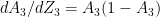
The equation for the backward propagation have the general form
$\partial L/\partial A_{l} = \partial L/\partial Z_{l+1} * W^{l+1}$
$\partial L/\partial Z_{l}=\partial L/\partial A_{l} *g'(Z_{l})$
$\partial L/\partial W_{l} =\partial L/\partial Z_{l} *A^{l-1}$
$\partial L/\partial b_{l} =\partial L/\partial Z_{l}$

Some other important results The derivatives of the activation functions in the implemented Deep Learning network
g(z) = sigmoid(z) = $1/(1+e^{-z})$ = a g’(z) = a(1-a) – See Part 1
g(z) = tanh(z) = a g’(z) = $1 - a^{2}$
g(z) = relu(z) = z when z>0 and 0 when z 0 and 0 when z <= 0
While it appears that there is a discontinuity for the derivative at 0 the small value at the discontinuity does not present a problem

The implementation of the multi layer vectorized Deep Learning Network for Python, R and Octave is included below. For all these implementations, initially I create the size and configuration of the the Deep Learning network with the layer dimennsions So for example layersDimension Vector ‘V’ of length L indicating ‘L’ layers where

V (in Python)= $[v_{0}, v_{1}, v_{2}$ , … $v_{L-1}]$
V (in R)= $c(v_{1}, v_{2}, v_{3}$ , … $v_{L})$
V (in Octave)= [ $v_{1} v_{2} v_{3}$ … $v_{L}]$

In all of these implementations the first element is the number of input features to the Deep Learning network and the last element is always a ‘sigmoid’ activation function since all the problems deal with binary classification.

The number of elements between the first and the last element are the number of hidden layers and the magnitude of each $v_{i}$ is the number of activation units in each hidden layer, which is specified while actually executing the Deep Learning network using the function L_Layer_DeepModel(), in all the implementations Python, R and Octave

1a. Classification with Multi layer Deep Learning Network – Relu activation(Python)

In the code below a 4 layer Neural Network is trained to generate a non-linear boundary between the classes. In the code below the ‘Relu’ Activation function is used. The number of activation units in each layer is 9. The cost vs iterations is plotted in addition to the decision boundary. Further the accuracy, precision, recall and F1 score are also computed

import os
import numpy as np
import matplotlib.pyplot as plt
import matplotlib.colors
import sklearn.linear_model

from sklearn.model_selection import train_test_split
from sklearn.datasets import make_classification, make_blobs
from matplotlib.colors import ListedColormap
import sklearn
import sklearn.datasets

#from DLfunctions import plot_decision_boundary
execfile("./DLfunctions34.py") # 
os.chdir("C:\\software\\DeepLearning-Posts\\part3")

# Create clusters of 2 classes
X1, Y1 = make_blobs(n_samples = 400, n_features = 2, centers = 9,
                       cluster_std = 1.3, random_state = 4)
#Create 2 classes
Y1=Y1.reshape(400,1)
Y1 = Y1 % 2
X2=X1.T
Y2=Y1.T
# Set the dimensions of DL Network 
#  Below we have 
#  2 - 2 input features
#  9,9 - 2 hidden layers with 9 activation units per layer and
#  1 - 1 sigmoid activation unit in the output layer as this is a binary classification
# The activation in the hidden layer is the 'relu' specified in L_Layer_DeepModel

layersDimensions = [2, 9, 9,1] #  4-layer model
parameters = L_Layer_DeepModel(X2, Y2, layersDimensions,hiddenActivationFunc='relu', learning_rate = 0.3,num_iterations = 2500, fig="fig1.png")
#Plot the decision boundary
plot_decision_boundary(lambda x: predict(parameters, x.T), X2,Y2,str(0.3),"fig2.png")

# Compute the confusion matrix
yhat = predict(parameters,X2)
from sklearn.metrics import confusion_matrix
a=confusion_matrix(Y2.T,yhat.T)
from sklearn.metrics import accuracy_score, precision_score, recall_score, f1_score
print('Accuracy: {:.2f}'.format(accuracy_score(Y2.T, yhat.T)))
print('Precision: {:.2f}'.format(precision_score(Y2.T, yhat.T)))
print('Recall: {:.2f}'.format(recall_score(Y2.T, yhat.T)))
print('F1: {:.2f}'.format(f1_score(Y2.T, yhat.T)))
## Accuracy: 0.90
## Precision: 0.91
## Recall: 0.87
## F1: 0.89

For more details on metrics like Accuracy, Recall, Precision etc. used in classification take a look at my post Practical Machine Learning with R and Python – Part 2. More details about these and other metrics besides implementation of the most common machine learning algorithms are available in my book My book ‘Practical Machine Learning with R and Python’ on Amazon

1b. Classification with Multi layer Deep Learning Network – Relu activation(R)

In the code below, binary classification is performed on the same data set as above using the Relu activation function. The DL network is same as above

library(ggplot2)
# Read the data
z <- as.matrix(read.csv("data.csv",header=FALSE)) 
x <- z[,1:2]
y <- z[,3]
X1 <- t(x)
Y1 <- t(y)

# Set the dimensions of the Deep Learning network
# No of input features =2, 2 hidden layers with 9 activation units and 1 output layer
layersDimensions = c(2, 9, 9,1)
# Execute the Deep Learning Neural Network
retvals = L_Layer_DeepModel(X1, Y1, layersDimensions,
                               hiddenActivationFunc='relu', 
                               learningRate = 0.3,
                               numIterations = 5000, 
                               print_cost = True)

library(ggplot2)
source("DLfunctions33.R")
# Get the computed costs
costs <- retvals[['costs']]
# Create a sequence of iterations
numIterations=5000
iterations <- seq(0,numIterations,by=1000)
df <-data.frame(iterations,costs)
# Plot the Costs vs number of iterations
ggplot(df,aes(x=iterations,y=costs)) + geom_point() +geom_line(color="blue") +
    xlab('No of iterations') + ylab('Cost') + ggtitle("Cost vs No of iterations")

# Plot the decision boundary
plotDecisionBoundary(z,retvals,hiddenActivationFunc="relu",0.3)

library(caret)

# Predict the output for the data values
yhat <-predict(retvals$parameters,X1,hiddenActivationFunc="relu")
yhat[yhat==FALSE]=0
yhat[yhat==TRUE]=1
# Compute the confusion matrix
confusionMatrix(yhat,Y1)

## Confusion Matrix and Statistics
## 
##           Reference
## Prediction   0   1
##          0 201  10
##          1  21 168
##                                           
##                Accuracy : 0.9225          
##                  95% CI : (0.8918, 0.9467)
##     No Information Rate : 0.555           
##     P-Value [Acc > NIR] : < 2e-16         
##                                           
##                   Kappa : 0.8441          
##  Mcnemar's Test P-Value : 0.07249         
##                                           
##             Sensitivity : 0.9054          
##             Specificity : 0.9438          
##          Pos Pred Value : 0.9526          
##          Neg Pred Value : 0.8889          
##              Prevalence : 0.5550          
##          Detection Rate : 0.5025          
##    Detection Prevalence : 0.5275          
##       Balanced Accuracy : 0.9246          
##                                           
##        'Positive' Class : 0               
##

1c. Classification with Multi layer Deep Learning Network – Relu activation(Octave)

Included below is the code for performing classification. Incidentally Octave does not seem to have implemented the confusion matrix, but confusionmat is available in Matlab.# Read the data data=csvread("data.csv"); X=data(:,1:2); Y=data(:,3); # Set layer dimensions layersDimensions = [2 9 7 1] #tanh=-0.5(ok), #relu=0.1 best! # Execute Deep Network [weights biases costs]=L_Layer_DeepModel(X', Y', layersDimensions, hiddenActivationFunc='relu', learningRate = 0.1, numIterations = 10000); plotCostVsIterations(10000,costs); plotDecisionBoundary(data,weights, biases,hiddenActivationFunc="tanh")

2a. Classification with Multi layer Deep Learning Network – Tanh activation(Python)

Below the Tanh activation function is used to perform the same classification. I found the Tanh activation required a simpler Neural Network of 3 layers.

# Tanh activation
import os
import numpy as np
import matplotlib.pyplot as plt
import matplotlib.colors
import sklearn.linear_model

from sklearn.model_selection import train_test_split
from sklearn.datasets import make_classification, make_blobs
from matplotlib.colors import ListedColormap
import sklearn
import sklearn.datasets

#from DLfunctions import plot_decision_boundary
os.chdir("C:\\software\\DeepLearning-Posts\\part3")
execfile("./DLfunctions34.py") 
# Create the dataset
X1, Y1 = make_blobs(n_samples = 400, n_features = 2, centers = 9,
                       cluster_std = 1.3, random_state = 4)
#Create 2 classes
Y1=Y1.reshape(400,1)
Y1 = Y1 % 2
X2=X1.T
Y2=Y1.T
# Set the dimensions of the Neural Network
layersDimensions = [2, 4, 1] #  3-layer model
# Compute the DL network
parameters = L_Layer_DeepModel(X2, Y2, layersDimensions, hiddenActivationFunc='tanh', learning_rate = .5,num_iterations = 2500,fig="fig3.png")
#Plot the decision boundary
plot_decision_boundary(lambda x: predict(parameters, x.T), X2,Y2,str(0.5),"fig4.png")

2b. Classification with Multi layer Deep Learning Network – Tanh activation(R)

R performs better with a Tanh activation than the Relu as can be seen below

 #Set the dimensions of the Neural Network
layersDimensions = c(2, 9, 9,1)
library(ggplot2)
# Read the data
z <- as.matrix(read.csv("data.csv",header=FALSE)) 
x <- z[,1:2]
y <- z[,3]
X1 <- t(x)
Y1 <- t(y)
# Execute the Deep Model
retvals = L_Layer_DeepModel(X1, Y1, layersDimensions,
                            hiddenActivationFunc='tanh', 
                            learningRate = 0.3,
                            numIterations = 5000, 
                            print_cost = True)

# Get the costs
costs <- retvals[['costs']]
iterations <- seq(0,numIterations,by=1000)
df <-data.frame(iterations,costs)
# Plot Cost vs number of iterations
ggplot(df,aes(x=iterations,y=costs)) + geom_point() +geom_line(color="blue") +
    xlab('No of iterations') + ylab('Cost') + ggtitle("Cost vs No of iterations")

#Plot the decision boundary
plotDecisionBoundary(z,retvals,hiddenActivationFunc="tanh",0.3)

2c. Classification with Multi layer Deep Learning Network – Tanh activation(Octave)

The code below uses the Tanh activation in the hidden layers for Octave# Read the data data=csvread("data.csv"); X=data(:,1:2); Y=data(:,3); # Set layer dimensions layersDimensions = [2 9 7 1] #tanh=-0.5(ok), #relu=0.1 best! # Execute Deep Network [weights biases costs]=L_Layer_DeepModel(X', Y', layersDimensions, hiddenActivationFunc='tanh', learningRate = 0.1, numIterations = 10000); plotCostVsIterations(10000,costs); plotDecisionBoundary(data,weights, biases,hiddenActivationFunc="tanh")

3. Bernoulli’s Lemniscate

To make things more interesting, I create a 2D figure of the Bernoulli’s lemniscate to perform non-linear classification. The Lemniscate is given by the equation
$(x^{2} + y^{2})^{2}$ = $2a^{2}*(x^{2}-y^{2})$

3a. Classifying a lemniscate with Deep Learning Network – Relu activation(Python)

import os
import numpy as np 
import matplotlib.pyplot as plt
os.chdir("C:\\software\\DeepLearning-Posts\\part3")
execfile("./DLfunctions33.py") 
x1=np.random.uniform(0,10,2000).reshape(2000,1)
x2=np.random.uniform(0,10,2000).reshape(2000,1)

X=np.append(x1,x2,axis=1)
X.shape

# Create a subset of values where squared is <0,4. Perform ravel() to flatten this vector
# Create the equation
# (x^{2} + y^{2})^2 - 2a^2*(x^{2}-y^{2}) <= 0
a=np.power(np.power(X[:,0]-5,2) + np.power(X[:,1]-5,2),2)
b=np.power(X[:,0]-5,2) - np.power(X[:,1]-5,2)
c= a - (b*np.power(4,2)) <=0
Y=c.reshape(2000,1)
# Create a scatter plot of the lemniscate
plt.scatter(X[:,0], X[:,1], c=Y, marker= 'o', s=15,cmap="viridis")
Z=np.append(X,Y,axis=1)
plt.savefig("fig50.png",bbox_inches='tight')
plt.clf()

# Set the data for classification
X2=X.T
Y2=Y.T
# These settings work the best
# Set the Deep Learning layer dimensions for a Relu activation
layersDimensions = [2,7,4,1]
#Execute the DL network
parameters = L_Layer_DeepModel(X2, Y2, layersDimensions, hiddenActivationFunc='relu', learning_rate = 0.5,num_iterations = 10000, fig="fig5.png")
#Plot the decision boundary
plot_decision_boundary(lambda x: predict(parameters, x.T), X2, Y2,str(2.2),"fig6.png")

# Compute the Confusion matrix
yhat = predict(parameters,X2)
from sklearn.metrics import confusion_matrix
a=confusion_matrix(Y2.T,yhat.T)
from sklearn.metrics import accuracy_score, precision_score, recall_score, f1_score
print('Accuracy: {:.2f}'.format(accuracy_score(Y2.T, yhat.T)))
print('Precision: {:.2f}'.format(precision_score(Y2.T, yhat.T)))
print('Recall: {:.2f}'.format(recall_score(Y2.T, yhat.T)))
print('F1: {:.2f}'.format(f1_score(Y2.T, yhat.T)))
## Accuracy: 0.93
## Precision: 0.77
## Recall: 0.76
## F1: 0.76

We could get better performance by tuning further. Do play around if you fork the code.
Note:: The lemniscate data is saved as a CSV and then read in R and also in Octave. I do this instead of recreating the lemniscate shape

3b. Classifying a lemniscate with Deep Learning Network – Relu activation(R code)

The R decision boundary for the Bernoulli’s lemniscate is shown below

Z <- as.matrix(read.csv("lemniscate.csv",header=FALSE))
Z1=data.frame(Z)
# Create a scatter plot of the lemniscate
ggplot(Z1,aes(x=V1,y=V2,col=V3)) +geom_point()

#Set the data for the DL network
X=Z[,1:2]
Y=Z[,3]

X1=t(X)
Y1=t(Y)

# Set the layer dimensions for the tanh activation function
layersDimensions = c(2,5,4,1)
# Execute the Deep Learning network with Tanh activation
retvals = L_Layer_DeepModel(X1, Y1, layersDimensions, 
                               hiddenActivationFunc='tanh', 
                               learningRate = 0.3,
                               numIterations = 20000, print_cost = True)

# Plot cost vs iteration
costs <- retvals[['costs']]
numIterations = 20000
iterations <- seq(0,numIterations,by=1000)
df <-data.frame(iterations,costs)
ggplot(df,aes(x=iterations,y=costs)) + geom_point() +geom_line(color="blue") +
    xlab('No of iterations') + ylab('Cost') + ggtitle("Cost vs No of iterations")

#Plot the decision boundary
plotDecisionBoundary(Z,retvals,hiddenActivationFunc="tanh",0.3)

3c. Classifying a lemniscate with Deep Learning Network – Relu activation(Octave code)

Octave is used to generate the non-linear lemniscate boundary.
# Read the data data=csvread("lemniscate.csv"); X=data(:,1:2); Y=data(:,3); # Set the dimensions of the layers layersDimensions = [2 9 7 1] # Compute the DL network [weights biases costs]=L_Layer_DeepModel(X', Y', layersDimensions, hiddenActivationFunc='relu', learningRate = 0.20, numIterations = 10000); plotCostVsIterations(10000,costs); plotDecisionBoundary(data,weights, biases,hiddenActivationFunc="relu")

4a. Binary Classification using MNIST – Python code

Finally I perform a simple classification using the MNIST handwritten digits, which according to Prof Geoffrey Hinton is “the Drosophila of Deep Learning”.

The Python code for reading the MNIST data is taken from Alex Kesling’s github link MNIST.

In the Python code below, I perform a simple binary classification between the handwritten digit ‘5’ and ‘not 5’ which is all other digits. I will perform the proper classification of all digits using the Softmax classifier some time later.

import os
import numpy as np 
import matplotlib.pyplot as plt
os.chdir("C:\\software\\DeepLearning-Posts\\part3")
execfile("./DLfunctions34.py") 
execfile("./load_mnist.py")
training=list(read(dataset='training',path="./mnist"))
test=list(read(dataset='testing',path="./mnist"))
lbls=[]
pxls=[]
print(len(training))

# Select the first 10000 training data and the labels
for i in range(10000):
       l,p=training[i]
       lbls.append(l)
       pxls.append(p)
labels= np.array(lbls)
pixels=np.array(pxls)   

#  Sey y=1  when labels == 5 and 0 otherwise
y=(labels==5).reshape(-1,1)
X=pixels.reshape(pixels.shape[0],-1)

# Create the necessary feature and target variable
X1=X.T
Y1=y.T

# Create the layer dimensions. The number of features are 28 x 28 = 784 since the 28 x 28
# pixels is flattened to single vector of length 784.
layersDimensions=[784, 15,9,7,1] # Works very well
parameters = L_Layer_DeepModel(X1, Y1, layersDimensions, hiddenActivationFunc='relu', learning_rate = 0.1,num_iterations = 1000, fig="fig7.png")

# Test data
lbls1=[]
pxls1=[]
for i in range(800):
       l,p=test[i]
       lbls1.append(l)
       pxls1.append(p)
 
testLabels=np.array(lbls1)
testData=np.array(pxls1)

ytest=(testLabels==5).reshape(-1,1)
Xtest=testData.reshape(testData.shape[0],-1)
Xtest1=Xtest.T
Ytest1=ytest.T

yhat = predict(parameters,Xtest1)
from sklearn.metrics import confusion_matrix
a=confusion_matrix(Ytest1.T,yhat.T)
from sklearn.metrics import accuracy_score, precision_score, recall_score, f1_score
print('Accuracy: {:.2f}'.format(accuracy_score(Ytest1.T, yhat.T)))
print('Precision: {:.2f}'.format(precision_score(Ytest1.T, yhat.T)))
print('Recall: {:.2f}'.format(recall_score(Ytest1.T, yhat.T)))
print('F1: {:.2f}'.format(f1_score(Ytest1.T, yhat.T)))

probs=predict_proba(parameters,Xtest1)
from sklearn.metrics import precision_recall_curve

precision, recall, thresholds = precision_recall_curve(Ytest1.T, probs.T)
closest_zero = np.argmin(np.abs(thresholds))
closest_zero_p = precision[closest_zero]
closest_zero_r = recall[closest_zero]
plt.xlim([0.0, 1.01])
plt.ylim([0.0, 1.01])
plt.plot(precision, recall, label='Precision-Recall Curve')
plt.plot(closest_zero_p, closest_zero_r, 'o', markersize = 12, fillstyle = 'none', c='r', mew=3)
plt.xlabel('Precision', fontsize=16)
plt.ylabel('Recall', fontsize=16)
plt.savefig("fig8.png",bbox_inches='tight')


## Accuracy: 0.99
## Precision: 0.96
## Recall: 0.89
## F1: 0.92

In addition to plotting the Cost vs Iterations, I also plot the Precision-Recall curve to show how the Precision and Recall, which are complementary to each other vary with respect to the other. To know more about Precision-Recall, please check my post Practical Machine Learning with R and Python – Part 4.

Check out my compact and minimal book “Practical Machine Learning with R and Python:Second edition- Machine Learning in stereo” available in Amazon in paperback($10.99) and kindle($7.99) versions. My book includes implementations of key ML algorithms and associated measures and metrics. The book is ideal for anybody who is familiar with the concepts and would like a quick reference to the different ML algorithms that can be applied to problems and how to select the best model. Pick your copy today!!

A physical copy of the book is much better than scrolling down a webpage. Personally, I tend to use my own book quite frequently to refer to R, Python constructs, subsetting, machine Learning function calls and the necessary parameters etc. It is useless to commit any of this to memory, and a physical copy of a book is much easier to thumb through for the relevant code snippet. Pick up your copy today!

4b. Binary Classification using MNIST – R code

In the R code below the same binary classification of the digit ‘5’ and the ‘not 5’ is performed. The code to read and display the MNIST data is taken from Brendan O’ Connor’s github link at MNIST

source("mnist.R")
load_mnist()
#show_digit(train$x[2,]
layersDimensions=c(784, 7,7,3,1) # Works at 1500
x <- t(train$x)
# Choose only 5000 training data
x2 <- x[,1:5000]
y <-train$y
# Set labels for all digits that are 'not 5' to 0
y[y!=5] <- 0
# Set labels of digit 5 as 1
y[y==5] <- 1
# Set the data
y1 <- as.matrix(y)
y2 <- t(y1)
# Choose the 1st 5000 data
y3 <- y2[,1:5000]

#Execute the Deep Learning Model
retvals = L_Layer_DeepModel(x2, y3, layersDimensions, 
                               hiddenActivationFunc='tanh', 
                               learningRate = 0.3,
                               numIterations = 3000, print_cost = True)

# Plot cost vs iteration
costs <- retvals[['costs']]
numIterations = 3000
iterations <- seq(0,numIterations,by=1000)
df <-data.frame(iterations,costs)
ggplot(df,aes(x=iterations,y=costs)) + geom_point() +geom_line(color="blue") +
    xlab('No of iterations') + ylab('Cost') + ggtitle("Cost vs No of iterations")

# Compute probability scores
scores <- computeScores(retvals$parameters, x2,hiddenActivationFunc='relu')
a=y3==1
b=y3==0

# Compute probabilities of class 0 and class 1
class1=scores[a]
class0=scores[b]

# Plot ROC curve
pr <-pr.curve(scores.class0=class1,
        scores.class1=class0,
       curve=T)

plot(pr)

The AUC curve hugs the top left corner and hence the performance of the classifier is quite good.

4c. Binary Classification using MNIST – Octave code

This code to load MNIST data was taken from Daniel E blog.
Precision recall curves are available in Matlab but are yet to be implemented in Octave’s statistics package.
load('./mnist/mnist.txt.gz'); % load the dataset # Subset the 'not 5' digits a=(trainY != 5); # Subset '5' b=(trainY == 5); #make a copy of trainY #Set 'not 5' as 0 and '5' as 1 y=trainY; y(a)=0; y(b)=1; X=trainX(1:5000,:); Y=y(1:5000); # Set the dimensions of layer layersDimensions=[784, 7,7,3,1]; # Compute the DL network [weights biases costs]=L_Layer_DeepModel(X', Y', layersDimensions, hiddenActivationFunc='relu', learningRate = 0.1, numIterations = 5000);

Conclusion

It was quite a challenge coding a Deep Learning Network in Python, R and Octave. The Deep Learning network implementation, in this post,is the base Deep Learning network, without any of the regularization methods included. Here are some key learning that I got while playing with different multi-layer networks on different problems

a. Deep Learning Networks come with many levers, the hyper-parameters,
– learning rate
– activation unit
– number of hidden layers
– number of units per hidden layer
– number of iterations while performing gradient descent
b. Deep Networks are very sensitive. A change in any of the hyper-parameter makes it perform very differently
c. Initially I thought adding more hidden layers, or more units per hidden layer will make the DL network better at learning. On the contrary, there is a performance degradation after the optimal DL configuration
d. At a sub-optimal number of hidden layers or number of hidden units, gradient descent seems to get stuck at a local minima
e. There were occasions when the cost came down, only to increase slowly as the number of iterations were increased. Probably early stopping would have helped.
f. I also did come across situations of ‘exploding/vanishing gradient’, cost went to Inf/-Inf. Here I would think inclusion of ‘momentum method’ would have helped

I intend to add the additional hyper-parameters of L1, L2 regularization, momentum method, early stopping etc. into the code in my future posts.
Feel free to fork/clone the code from Github Deep Learning – Part 3, and take the DL network apart and play around with it.

I will be continuing this series with more hyper-parameters to handle vanishing and exploding gradients, early stopping and regularization in the weeks to come. I also intend to add some more activation functions to this basic Multi-Layer Network.
Hang around, there are more exciting things to come.

Watch this space!

References
1. Deep Learning Specialization
2. Neural Networks for Machine Learning
3. Deep Learning, Ian Goodfellow, Yoshua Bengio and Aaron Courville
4. Neural Networks: The mechanics of backpropagation
5. Machine Learning

Also see
1.My book ‘Practical Machine Learning with R and Python’ on Amazon
2. My travels through the realms of Data Science, Machine Learning, Deep Learning and (AI)
3. Designing a Social Web Portal
4. GooglyPlus: yorkr analyzes IPL players, teams, matches with plots and tables
4. Introducing QCSimulator: A 5-qubit quantum computing simulator in R
6. Presentation on “Intelligent Networks, CAMEL protocol, services & applications
7. Design Principles of Scalable, Distributed Systems

To see all posts see Index of posts

Deep Learning from first principles in Python, R and Octave – Part 2

“What does the world outside your head really ‘look’ like? Not only is there no color, there’s also no sound: the compression and expansion of air is picked up by the ears, and turned into electrical signals. The brain then presents these signals to us as mellifluous tones and swishes and clatters and jangles. Reality is also odorless: there’s no such thing as smell outside our brains. Molecules floating through the air bind to receptors in our nose and are interpreted as different smells by our brain. The real world is not full of rich sensory events; instead, our brains light up the world with their own sensuality.”
The Brain: The Story of You” by David Eagleman

“The world is Maya, illusory. The ultimate reality, the Brahman, is all-pervading and all-permeating, which is colourless, odourless, tasteless, nameless and formless“
Bhagavad Gita

1. Introduction

This post is a follow-up post to my earlier post Deep Learning from first principles in Python, R and Octave-Part 1. In the first part, I implemented Logistic Regression, in vectorized Python,R and Octave, with a wannabe Neural Network (a Neural Network with no hidden layers). In this second part, I implement a regular, but somewhat primitive Neural Network (a Neural Network with just 1 hidden layer). The 2nd part implements classification of manually created datasets, where the different clusters of the 2 classes are not linearly separable.

Neural Network perform really well in learning all sorts of non-linear boundaries between classes. Initially logistic regression is used perform the classification and the decision boundary is plotted. Vanilla logistic regression performs quite poorly. Using SVMs with a radial basis kernel would have performed much better in creating non-linear boundaries. To see R and Python implementations of SVMs take a look at my post Practical Machine Learning with R and Python – Part 4.

You may also like my companion book “Practical Machine Learning with R and Python:Second Edition- Machine Learning in stereo” available in Amazon in paperback($10.99) and Kindle($7.99/Rs449) versions. This book is ideal for a quick reference of the various ML functions and associated measurements in both R and Python which are essential to delve deep into Deep Learning.

Take a look at my video presentation which discusses the below derivation step-by- step Elements of Neural Networks and Deep Learning – Part 3

You can clone and fork this R Markdown file along with the vectorized implementations of the 3 layer Neural Network for Python, R and Octave from Github DeepLearning-Part2

2. The 3 layer Neural Network

A simple representation of a 3 layer Neural Network (NN) with 1 hidden layer is shown below.

In the above Neural Network, there are 2 input features at the input layer, 3 hidden units at the hidden layer and 1 output layer as it deals with binary classification. The activation unit at the hidden layer can be a tanh, sigmoid, relu etc. At the output layer the activation is a sigmoid to handle binary classification

# Superscript indicates layer 1
$z_{11} = w_{11}^{1}x_{1} + w_{21}^{1}x_{2} + b_{1}$
$z_{12} = w_{12}^{1}x_{1} + w_{22}^{1}x_{2} + b_{1}$
$z_{13} = w_{13}^{1}x_{1} + w_{23}^{1}x_{2} + b_{1}$

Also $a_{11} = tanh(z_{11})$
$a_{12} = tanh(z_{12})$
$a_{13} = tanh(z_{13})$

# Superscript indicates layer 2
$z_{21} = w_{11}^{2}a_{11} + w_{21}^{2}a_{12} + w_{31}^{2}a_{13} + b_{2}$
$a_{21} = sigmoid(z21)$

Hence
$Z1= \begin{pmatrix} z11\\ z12\\ z13 \end{pmatrix} =\begin{pmatrix} w_{11}^{1} & w_{21}^{1} \\ w_{12}^{1} & w_{22}^{1} \\ w_{13}^{1} & w_{23}^{1} \end{pmatrix} * \begin{pmatrix} x1\\ x2 \end{pmatrix} + b_{1}$
And
$A1= \begin{pmatrix} a11\\ a12\\ a13 \end{pmatrix} = \begin{pmatrix} tanh(z11)\\ tanh(z12)\\ tanh(z13) \end{pmatrix}$

Similarly
$Z2= z_{21} = \begin{pmatrix} w_{11}^{2} & w_{21}^{2} & w_{31}^{2} \end{pmatrix} *\begin{pmatrix} z_{11}\\ z_{12}\\ z_{13} \end{pmatrix} +b_{2}$
and $A2 = a_{21} = sigmoid(z_{21})$

These equations can be written as
$Z1 = W1 * X + b1$
$A1 = tanh(Z1)$
$Z2 = W2 * A1 + b2$
$A2 = sigmoid(Z2)$

I) Some important results (a memory refresher!)
$d/dx(e^{x}) = e^{x}$ and $d/dx(e^{-x}) = -e^{-x}$ -(a) and
$sinhx = (e^{x} - e^{-x})/2$ and $coshx = (e^{x} + e^{-x})/2$
Using (a) we can shown that $d/dx(sinhx) = coshx$ and $d/dx(coshx) = sinhx$ (b)
Now $d/dx(f(x)/g(x)) = (g(x)*d/dx(f(x)) - f(x)*d/dx(g(x)))/g(x)^{2}$ -(c)

Since $tanhx =z= sinhx/coshx$ and using (b) we get
$tanhx = (coshx*d/dx(sinhx) - sinhx*d/dx(coshx))/(cosh^{2})$
Using the values of the derivatives of sinhx and coshx from (b) above we get
$d/dx(tanhx) = (coshx^{2} - sinhx{2})/coshx{2} = 1 - tanhx^{2}$
Since $tanhx =z$
$d/dx(tanhx) = 1 - tanhx^{2}= 1 - z^{2}$ -(d)

II) Derivatives
$L=-(Ylog(A2) + (1-Y)log(1-A2))$
$dL/dA2 = -(Y/A2 + (1-Y)/(1-A2))$
Since $A2 = sigmoid(Z2)$ therefore $dA2/dZ2 = A2(1-A2)$ see Part1
$Z2 = W2A1 +b2$
$dZ2/dW2 = A1$
$dZ2/db2 = 1$
$A1 = tanh(Z1)$ and $dA1/dZ1 = 1 - A1^{2}$
$Z1 = W1X + b1$
$dZ1/dW1 = X$
$dZ1/db1 = 1$

III) Back propagation
Using the derivatives from II) we can derive the following results using Chain Rule
$\partial L/\partial Z2 = \partial L/\partial A2 * \partial A2/\partial Z2$
$= -(Y/A2 + (1-Y)/(1-A2)) * A2(1-A2) = A2 - Y$
$\partial L/\partial W2 = \partial L/\partial A2 * \partial A2/\partial Z2 * \partial Z2/\partial W2$
$= (A2-Y) *A1$ -(A)
$\partial L/\partial b2 = \partial L/\partial A2 * \partial A2/\partial Z2 * \partial Z2/\partial b2 = (A2-Y)$ -(B)

$\partial L/\partial Z1 = \partial L/\partial A2 * \partial A2/\partial Z2 * \partial Z2/\partial A1 *\partial A1/\partial Z1 = (A2-Y) * W2 * (1-A1^{2})$
$\partial L/\partial W1 = \partial L/\partial A2 * \partial A2/\partial Z2 * \partial Z2/\partial A1 *\partial A1/\partial Z1 *\partial Z1/\partial W1$
$=(A2-Y) * W2 * (1-A1^{2}) * X$ -(C)
$\partial L/\partial b1 = \partial L/\partial A2 * \partial A2/\partial Z2 * \partial Z2/\partial A1 *dA1/dZ1 *dZ1/db1$
$= (A2-Y) * W2 * (1-A1^{2})$ -(D)

IV) Gradient Descent
The key computations in the backward cycle are
$W1 = W1-learningRate * \partial L/\partial W1$ – From (C)
$b1 = b1-learningRate * \partial L/\partial b1$ – From (D)
$W2 = W2-learningRate * \partial L/\partial W2$ – From (A)
$b2 = b2-learningRate * \partial L/\partial b2$ – From (B)

The weights and biases (W1,b1,W2,b2) are updated for each iteration thus minimizing the loss/cost.

These derivations can be represented pictorially using the computation graph (from the book Deep Learning by Ian Goodfellow, Joshua Bengio and Aaron Courville)

3. Manually create a data set that is not lineary separable

Initially I create a dataset with 2 classes which has around 9 clusters that cannot be separated by linear boundaries. Note: This data set is saved as data.csv and is used for the R and Octave Neural networks to see how they perform on the same dataset.

import numpy as np
import matplotlib.pyplot as plt
import matplotlib.colors
import sklearn.linear_model

from sklearn.model_selection import train_test_split
from sklearn.datasets import make_classification, make_blobs
from matplotlib.colors import ListedColormap
import sklearn
import sklearn.datasets


colors=['black','gold']
cmap = matplotlib.colors.ListedColormap(colors)
X, y = make_blobs(n_samples = 400, n_features = 2, centers = 7,
                       cluster_std = 1.3, random_state = 4)
#Create 2 classes
y=y.reshape(400,1)
y = y % 2
#Plot the figure
plt.figure()
plt.title('Non-linearly separable classes')
plt.scatter(X[:,0], X[:,1], c=y,
           marker= 'o', s=50,cmap=cmap)
plt.savefig('fig1.png', bbox_inches='tight')

4. Logistic Regression

On the above created dataset, classification with logistic regression is performed, and the decision boundary is plotted. It can be seen that logistic regression performs quite poorly

import numpy as np
import matplotlib.pyplot as plt
import matplotlib.colors
import sklearn.linear_model

from sklearn.model_selection import train_test_split
from sklearn.datasets import make_classification, make_blobs
from matplotlib.colors import ListedColormap
import sklearn
import sklearn.datasets

#from DLfunctions import plot_decision_boundary
execfile("./DLfunctions.py") # Since import does not work in Rmd!!!

colors=['black','gold']
cmap = matplotlib.colors.ListedColormap(colors)
X, y = make_blobs(n_samples = 400, n_features = 2, centers = 7,
                       cluster_std = 1.3, random_state = 4)
#Create 2 classes
y=y.reshape(400,1)
y = y % 2

# Train the logistic regression classifier
clf = sklearn.linear_model.LogisticRegressionCV();
clf.fit(X, y);

# Plot the decision boundary for logistic regression
plot_decision_boundary_n(lambda x: clf.predict(x), X.T, y.T,"fig2.png")

5. The 3 layer Neural Network in Python (vectorized)

The vectorized implementation is included below. Note that in the case of Python a learning rate of 0.5 and 3 hidden units performs very well.

## Random data set with 9 clusters
import numpy as np
import matplotlib
import matplotlib.pyplot as plt
import sklearn.linear_model
import pandas as pd

from sklearn.datasets import make_classification, make_blobs
execfile("./DLfunctions.py") # Since import does not work in Rmd!!!

X1, Y1 = make_blobs(n_samples = 400, n_features = 2, centers = 9,
                       cluster_std = 1.3, random_state = 4)
#Create 2 classes
Y1=Y1.reshape(400,1)
Y1 = Y1 % 2
X2=X1.T
Y2=Y1.T

#Perform gradient descent
parameters,costs = computeNN(X2, Y2, numHidden = 4, learningRate=0.5, numIterations = 10000)
plot_decision_boundary(lambda x: predict(parameters, x.T), X2, Y2,str(4),str(0.5),"fig3.png")

## Cost after iteration 0: 0.692669
## Cost after iteration 1000: 0.246650
## Cost after iteration 2000: 0.227801
## Cost after iteration 3000: 0.226809
## Cost after iteration 4000: 0.226518
## Cost after iteration 5000: 0.226331
## Cost after iteration 6000: 0.226194
## Cost after iteration 7000: 0.226085
## Cost after iteration 8000: 0.225994
## Cost after iteration 9000: 0.225915

6. The 3 layer Neural Network in R (vectorized)

For this the dataset created by Python is saved to see how R performs on the same dataset. The vectorized implementation of a Neural Network was just a little more interesting as R does not have a similar package like ‘numpy’. While numpy handles broadcasting implicitly, in R I had to use the ‘sweep’ command to broadcast. The implementaion is included below. Note that since the initialization with random weights is slightly different, R performs best with a learning rate of 0.1 and with 6 hidden units

source("DLfunctions2_1.R")

z <- as.matrix(read.csv("data.csv",header=FALSE)) # 
x <- z[,1:2]
y <- z[,3]
x1 <- t(x)
y1 <- t(y)
#Perform gradient descent
nn <-computeNN(x1, y1, 6, learningRate=0.1,numIterations=10000) # Good

## [1] 0.7075341
## [1] 0.2606695
## [1] 0.2198039
## [1] 0.2091238
## [1] 0.211146
## [1] 0.2108461
## [1] 0.2105351
## [1] 0.210211
## [1] 0.2099104
## [1] 0.2096437
## [1] 0.209409

plotDecisionBoundary(z,nn,6,0.1)

7. The 3 layer Neural Network in Octave (vectorized)

This uses the same dataset that was generated using Python code.
source("DL-function2.m") data=csvread("data.csv"); X=data(:,1:2); Y=data(:,3); # Make sure that the model parameters are correct. Take the transpose of X & Y
#Perform gradient descent [W1,b1,W2,b2,costs]= computeNN(X', Y',4, learningRate=0.5, numIterations = 10000);

8a. Performance for different learning rates (Python)

import numpy as np
import matplotlib
import matplotlib.pyplot as plt
import sklearn.linear_model
import pandas as pd

from sklearn.datasets import make_classification, make_blobs
execfile("./DLfunctions.py") # Since import does not work in Rmd!!!
# Create data
X1, Y1 = make_blobs(n_samples = 400, n_features = 2, centers = 9,
                       cluster_std = 1.3, random_state = 4)
#Create 2 classes
Y1=Y1.reshape(400,1)
Y1 = Y1 % 2
X2=X1.T
Y2=Y1.T
# Create a list of learning rates
learningRate=[0.5,1.2,3.0]
df=pd.DataFrame()
#Compute costs for each learning rate
for lr in learningRate:
   parameters,costs = computeNN(X2, Y2, numHidden = 4, learningRate=lr, numIterations = 10000)
   print(costs)
   df1=pd.DataFrame(costs)
   df=pd.concat([df,df1],axis=1)
#Set the iterations
iterations=[0,1000,2000,3000,4000,5000,6000,7000,8000,9000]   
#Create data frame
#Set index
df1=df.set_index([iterations])
df1.columns=[0.5,1.2,3.0]
fig=df1.plot()
fig=plt.title("Cost vs No of Iterations for different learning rates")
plt.savefig('fig4.png', bbox_inches='tight')

8b. Performance for different hidden units (Python)

import numpy as np
import matplotlib
import matplotlib.pyplot as plt
import sklearn.linear_model
import pandas as pd

from sklearn.datasets import make_classification, make_blobs
execfile("./DLfunctions.py") # Since import does not work in Rmd!!!
#Create data set
X1, Y1 = make_blobs(n_samples = 400, n_features = 2, centers = 9,
                       cluster_std = 1.3, random_state = 4)
#Create 2 classes
Y1=Y1.reshape(400,1)
Y1 = Y1 % 2
X2=X1.T
Y2=Y1.T
# Make a list of hidden unis
numHidden=[3,5,7]
df=pd.DataFrame()
#Compute costs for different hidden units
for numHid in numHidden:
   parameters,costs = computeNN(X2, Y2, numHidden = numHid, learningRate=1.2, numIterations = 10000)
   print(costs)
   df1=pd.DataFrame(costs)
   df=pd.concat([df,df1],axis=1)
#Set the iterations
iterations=[0,1000,2000,3000,4000,5000,6000,7000,8000,9000]   
#Set index
df1=df.set_index([iterations])
df1.columns=[3,5,7]
#Plot
fig=df1.plot()
fig=plt.title("Cost vs No of Iterations for different no of hidden units")
plt.savefig('fig5.png', bbox_inches='tight')

9a. Performance for different learning rates (R)

source("DLfunctions2_1.R")
# Read data
z <- as.matrix(read.csv("data.csv",header=FALSE)) # 
x <- z[,1:2]
y <- z[,3]
x1 <- t(x)
y1 <- t(y)
#Loop through learning rates and compute costs
learningRate <-c(0.1,1.2,3.0)
df <- NULL
for(i in seq_along(learningRate)){
   nn <-  computeNN(x1, y1, 6, learningRate=learningRate[i],numIterations=10000) 
   cost <- nn$costs
   df <- cbind(df,cost)
  
}


#Create dataframe
df <- data.frame(df) 
iterations=seq(0,10000,by=1000)
df <- cbind(iterations,df)
names(df) <- c("iterations","0.5","1.2","3.0")
library(reshape2)

df1 <- melt(df,id="iterations")  # Melt the data
#Plot  
ggplot(df1) + geom_line(aes(x=iterations,y=value,colour=variable),size=1)  + 
    xlab("Iterations") +
    ylab('Cost') + ggtitle("Cost vs No iterations for  different learning rates")

9b. Performance for different hidden units (R)

source("DLfunctions2_1.R")
# Loop through Num hidden units
numHidden <-c(4,6,9)
df <- NULL
for(i in seq_along(numHidden)){
    nn <-  computeNN(x1, y1, numHidden[i], learningRate=0.1,numIterations=10000) 
    cost <- nn$costs
    df <- cbind(df,cost)
    
}

df <- data.frame(df) 
iterations=seq(0,10000,by=1000)
df <- cbind(iterations,df)
names(df) <- c("iterations","4","6","9")
library(reshape2)
# Melt
df1 <- melt(df,id="iterations") 
# Plot   
ggplot(df1) + geom_line(aes(x=iterations,y=value,colour=variable),size=1)  + 
    xlab("Iterations") +
    ylab('Cost') + ggtitle("Cost vs No iterations for  different number of hidden units")

10a. Performance of the Neural Network for different learning rates (Octave)

source("DL-function2.m") plotLRCostVsIterations() print -djph figa.jpg

10b. Performance of the Neural Network for different number of hidden units (Octave)

source("DL-function2.m") plotHiddenCostVsIterations() print -djph figa.jpg

11. Turning the heat on the Neural Network

In this 2nd part I create a a central region of positives and and the outside region as negatives. The points are generated using the equation of a circle (x – a)^{2} + (y -b) ^{2} = R^{2} . How does the 3 layer Neural Network perform on this? Here’s a look! Note: The same dataset is also used for R and Octave Neural Network constructions

12. Manually creating a circular central region

import numpy as np
import matplotlib.pyplot as plt
import matplotlib.colors
import sklearn.linear_model

from sklearn.model_selection import train_test_split
from sklearn.datasets import make_classification, make_blobs
from matplotlib.colors import ListedColormap
import sklearn
import sklearn.datasets

colors=['black','gold']
cmap = matplotlib.colors.ListedColormap(colors)
x1=np.random.uniform(0,10,800).reshape(800,1)
x2=np.random.uniform(0,10,800).reshape(800,1)
X=np.append(x1,x2,axis=1)
X.shape
# Create (x-a)^2 + (y-b)^2 = R^2
# Create a subset of values where squared is <0,4. Perform ravel() to flatten this vector
a=(np.power(X[:,0]-5,2) + np.power(X[:,1]-5,2) <= 6).ravel()
Y=a.reshape(800,1)

cmap = matplotlib.colors.ListedColormap(colors)

plt.figure()
plt.title('Non-linearly separable classes')
plt.scatter(X[:,0], X[:,1], c=Y,
           marker= 'o', s=15,cmap=cmap)
plt.savefig('fig6.png', bbox_inches='tight')

13a. Decision boundary with hidden units=4 and learning rate = 2.2 (Python)

With the above hyper parameters the decision boundary is triangular

import numpy as np
import matplotlib.pyplot as plt
import matplotlib.colors
import sklearn.linear_model
execfile("./DLfunctions.py")
x1=np.random.uniform(0,10,800).reshape(800,1)
x2=np.random.uniform(0,10,800).reshape(800,1)
X=np.append(x1,x2,axis=1)
X.shape

# Create a subset of values where squared is <0,4. Perform ravel() to flatten this vector
a=(np.power(X[:,0]-5,2) + np.power(X[:,1]-5,2) <= 6).ravel()
Y=a.reshape(800,1)

X2=X.T
Y2=Y.T

parameters,costs = computeNN(X2, Y2, numHidden = 4, learningRate=2.2, numIterations = 10000)
plot_decision_boundary(lambda x: predict(parameters, x.T), X2, Y2,str(4),str(2.2),"fig7.png")

## Cost after iteration 0: 0.692836
## Cost after iteration 1000: 0.331052
## Cost after iteration 2000: 0.326428
## Cost after iteration 3000: 0.474887
## Cost after iteration 4000: 0.247989
## Cost after iteration 5000: 0.218009
## Cost after iteration 6000: 0.201034
## Cost after iteration 7000: 0.197030
## Cost after iteration 8000: 0.193507
## Cost after iteration 9000: 0.191949

13b. Decision boundary with hidden units=12 and learning rate = 2.2 (Python)

With the above hyper parameters the decision boundary is triangular

import numpy as np
import matplotlib.pyplot as plt
import matplotlib.colors
import sklearn.linear_model
execfile("./DLfunctions.py")
x1=np.random.uniform(0,10,800).reshape(800,1)
x2=np.random.uniform(0,10,800).reshape(800,1)
X=np.append(x1,x2,axis=1)
X.shape

# Create a subset of values where squared is <0,4. Perform ravel() to flatten this vector
a=(np.power(X[:,0]-5,2) + np.power(X[:,1]-5,2) <= 6).ravel()
Y=a.reshape(800,1)

X2=X.T
Y2=Y.T

parameters,costs = computeNN(X2, Y2, numHidden = 12, learningRate=2.2, numIterations = 10000)
plot_decision_boundary(lambda x: predict(parameters, x.T), X2, Y2,str(12),str(2.2),"fig8.png")

## Cost after iteration 0: 0.693291
## Cost after iteration 1000: 0.383318
## Cost after iteration 2000: 0.298807
## Cost after iteration 3000: 0.251735
## Cost after iteration 4000: 0.177843
## Cost after iteration 5000: 0.130414
## Cost after iteration 6000: 0.152400
## Cost after iteration 7000: 0.065359
## Cost after iteration 8000: 0.050921
## Cost after iteration 9000: 0.039719

14a. Decision boundary with hidden units=9 and learning rate = 0.5 (R)

When the number of hidden units is 6 and the learning rate is 0,1, is also a triangular shape in R

source("DLfunctions2_1.R")
z <- as.matrix(read.csv("data1.csv",header=FALSE)) # N
x <- z[,1:2]
y <- z[,3]
x1 <- t(x)
y1 <- t(y)
nn <-computeNN(x1, y1, 9, learningRate=0.5,numIterations=10000) # Triangular

## [1] 0.8398838
## [1] 0.3303621
## [1] 0.3127731
## [1] 0.3012791
## [1] 0.3305543
## [1] 0.3303964
## [1] 0.2334615
## [1] 0.1920771
## [1] 0.2341225
## [1] 0.2188118
## [1] 0.2082687

plotDecisionBoundary(z,nn,6,0.1)

14b. Decision boundary with hidden units=8 and learning rate = 0.1 (R)

source("DLfunctions2_1.R")
z <- as.matrix(read.csv("data1.csv",header=FALSE)) # N
x <- z[,1:2]
y <- z[,3]
x1 <- t(x)
y1 <- t(y)
nn <-computeNN(x1, y1, 8, learningRate=0.1,numIterations=10000) # Hemisphere

## [1] 0.7273279
## [1] 0.3169335
## [1] 0.2378464
## [1] 0.1688635
## [1] 0.1368466
## [1] 0.120664
## [1] 0.111211
## [1] 0.1043362
## [1] 0.09800573
## [1] 0.09126161
## [1] 0.0840379

plotDecisionBoundary(z,nn,8,0.1)

15a. Decision boundary with hidden units=12 and learning rate = 1.5 (Octave)

source("DL-function2.m") data=csvread("data1.csv"); X=data(:,1:2); Y=data(:,3); # Make sure that the model parameters are correct. Take the transpose of X & Y [W1,b1,W2,b2,costs]= computeNN(X', Y',12, learningRate=1.5, numIterations = 10000); plotDecisionBoundary(data, W1,b1,W2,b2) print -djpg fige.jpg

Conclusion: This post implemented a 3 layer Neural Network to create non-linear boundaries while performing classification. Clearly the Neural Network performs very well when the number of hidden units and learning rate are varied.

To be continued…
Watch this space!!

Also see
1. My book ‘Practical Machine Learning with R and Python’ on Amazon
2. GooglyPlus: yorkr analyzes IPL players, teams, matches with plots and tables
3. The 3rd paperback & kindle editions of my books on Cricket, now on Amazon
4. Exploring Quantum Gate operations with QCSimulator
5. Simulating a Web Joint in Android
6. My travels through the realms of Data Science, Machine Learning, Deep Learning and (AI)
7. Presentation on Wireless Technologies – Part 1

To see all posts check Index of posts

Deep Learning from first principles in Python, R and Octave – Part 1

“You don’t perceive objects as they are. You perceive them as you are.”
“Your interpretation of physical objects has everything to do with the historical trajectory of your brain – and little to do with the objects themselves.”
“The brain generates its own reality, even before it receives information coming in from the eyes and the other senses. This is known as the internal model”

                          David Eagleman - The Brain: The Story of You

This is the first in the series of posts, I intend to write on Deep Learning. This post is inspired by the Deep Learning Specialization by Prof Andrew Ng on Coursera and Neural Networks for Machine Learning by Prof Geoffrey Hinton also on Coursera. In this post I implement Logistic regression with a 2 layer Neural Network i.e. a Neural Network that just has an input layer and an output layer and with no hidden layer.I am certain that any self-respecting Deep Learning/Neural Network would consider a Neural Network without hidden layers as no Neural Network at all!

This 2 layer network is implemented in Python, R and Octave languages. I have included Octave, into the mix, as Octave is a close cousin of Matlab. These implementations in Python, R and Octave are equivalent vectorized implementations. So, if you are familiar in any one of the languages, you should be able to look at the corresponding code in the other two. You can download this R Markdown file and Octave code from DeepLearning -Part 1

Check out my video presentation which discusses the derivations in detail
1. Elements of Neural Networks and Deep Le- Part 1
2. Elements of Neural Networks and Deep Learning – Part 2

To start with, Logistic Regression is performed using sklearn’s logistic regression package for the cancer data set also from sklearn. This is shown below

1. Logistic Regression

import numpy as np
import pandas as pd
import os
import matplotlib.pyplot as plt
from sklearn.model_selection import train_test_split
from sklearn.linear_model import LogisticRegression
from sklearn.datasets import make_classification, make_blobs

from sklearn.metrics import confusion_matrix
from matplotlib.colors import ListedColormap
from sklearn.datasets import load_breast_cancer
# Load the cancer data
(X_cancer, y_cancer) = load_breast_cancer(return_X_y = True)
X_train, X_test, y_train, y_test = train_test_split(X_cancer, y_cancer,
                                                   random_state = 0)
# Call the Logisitic Regression function
clf = LogisticRegression().fit(X_train, y_train)
print('Accuracy of Logistic regression classifier on training set: {:.2f}'
     .format(clf.score(X_train, y_train)))
print('Accuracy of Logistic regression classifier on test set: {:.2f}'
     .format(clf.score(X_test, y_test)))

## Accuracy of Logistic regression classifier on training set: 0.96
## Accuracy of Logistic regression classifier on test set: 0.96

To check on other classification algorithms, check my post Practical Machine Learning with R and Python – Part 2.

2. Logistic Regression as a 2 layer Neural Network

In the following section Logistic Regression is implemented as a 2 layer Neural Network in Python, R and Octave. The same cancer data set from sklearn will be used to train and test the Neural Network in Python, R and Octave. This can be represented diagrammatically as below

The cancer data set has 30 input features, and the target variable ‘output’ is either 0 or 1. Hence the sigmoid activation function will be used in the output layer for classification.

This simple 2 layer Neural Network is shown below
At the input layer there are 30 features and the corresponding weights of these inputs which are initialized to small random values.
$Z= w_{1}x_{1} +w_{2}x_{2} +..+ w_{30}x_{30} + b$
where ‘b’ is the bias term

The Activation function is the sigmoid function which is $a= 1/(1+e^{-z})$
The Loss, when the sigmoid function is used in the output layer, is given by
$L=-(ylog(a) + (1-y)log(1-a))$ (1)

Gradient Descent

Forward propagation

In forward propagation cycle of the Neural Network the output Z and the output of activation function, the sigmoid function, is first computed. Then using the output ‘y’ for the given features, the ‘Loss’ is computed using equation (1) above.

Backward propagation

The backward propagation cycle determines how the ‘Loss’ is impacted for small variations from the previous layers upto the input layer. In other words, backward propagation computes the changes in the weights at the input layer, which will minimize the loss. Several cycles of gradient descent are performed in the path of steepest descent to find the local minima. In other words the set of weights and biases, at the input layer, which will result in the lowest loss is computed by gradient descent. The weights at the input layer are decreased by a parameter known as the ‘learning rate’. Too big a ‘learning rate’ can overshoot the local minima, and too small a ‘learning rate’ can take a long time to reach the local minima. This is done for ‘m’ training examples.

Chain rule of differentiation
Let y=f(u)
and u=g(x) then
$\partial y/\partial x = \partial y/\partial u * \partial u/\partial x$

Derivative of sigmoid
$\sigma=1/(1+e^{-z})$
Let $x= 1 + e^{-z}$ then
$\sigma = 1/x$
$\partial \sigma/\partial x = -1/x^{2}$
$\partial x/\partial z = -e^{-z}$
Using the chain rule of differentiation we get
$\partial \sigma/\partial z = \partial \sigma/\partial x * \partial x/\partial z$
$=-1/(1+e^{-z})^{2}* -e^{-z} = e^{-z}/(1+e^{-z})^{2}$
Therefore $\partial \sigma/\partial z = \sigma(1-\sigma)$ -(2)

The 3 equations for the 2 layer Neural Network representation of Logistic Regression are
$L=-(y*log(a) + (1-y)*log(1-a))$ -(a)
$a=1/(1+e^{-Z})$ -(b)
$Z= w_{1}x_{1} +w_{2}x_{2} +...+ w_{30}x_{30} +b = Z = \sum_{i} w_{i}*x_{i} + b$ -(c)

The back propagation step requires the computation of $dL/dw_{i}$ and $dL/db_{i}$ . In the case of regression it would be $dE/dw_{i}$ and $dE/db_{i}$ where dE is the Mean Squared Error function.
Computing the derivatives for back propagation we have
$dL/da = -(y/a + (1-y)/(1-a))$ -(d)
because $d/dx(logx) = 1/x$
Also from equation (2) we get
$da/dZ = a (1-a)$ – (e)
By chain rule
$\partial L/\partial Z = \partial L/\partial a * \partial a/\partial Z$
therefore substituting the results of (d) & (e) we get
$\partial L/\partial Z = -(y/a + (1-y)/(1-a)) * a(1-a) = a-y$ (f)
Finally
$\partial L/\partial w_{i}= \partial L/\partial a * \partial a/\partial Z * \partial Z/\partial w_{i}$ -(g)
$\partial Z/\partial w_{i} = x_{i}$ – (h)
and from (f) we have $\partial L/\partial Z =a-y$
Therefore (g) reduces to
$\partial L/\partial w_{i} = x_{i}* (a-y)$ -(i)
Also
$\partial L/\partial b = \partial L/\partial a * \partial a/\partial Z * \partial Z/\partial b$ -(j)
Since
$\partial Z/\partial b = 1$ and using (f) in (j)
$\partial L/\partial b = a-y$

The gradient computes the weights at the input layer and the corresponding bias by using the values
of $dw_{i}$ and $db$
$w_{i} := w_{i} -\alpha * dw_{i}$
$b := b -\alpha * db$
I found the computation graph representation in the book Deep Learning: Ian Goodfellow, Yoshua Bengio, Aaron Courville, very useful to visualize and also compute the backward propagation. For the 2 layer Neural Network of Logistic Regression the computation graph is shown below

3. Neural Network for Logistic Regression -Python code (vectorized)

import numpy as np
import pandas as pd
import os
import matplotlib.pyplot as plt
from sklearn.model_selection import train_test_split

# Define the sigmoid function
def sigmoid(z):  
    a=1/(1+np.exp(-z))    
    return a

# Initialize
def initialize(dim):
    w = np.zeros(dim).reshape(dim,1)
    b = 0   
    return w

# Compute the loss
def computeLoss(numTraining,Y,A):
    loss=-1/numTraining *np.sum(Y*np.log(A) + (1-Y)*(np.log(1-A)))
    return(loss)

# Execute the forward propagation
def forwardPropagation(w,b,X,Y):
    # Compute Z
    Z=np.dot(w.T,X)+b
    # Determine the number of training samples
    numTraining=float(len(X))
    # Compute the output of the sigmoid activation function 
    A=sigmoid(Z)
    #Compute the loss
    loss = computeLoss(numTraining,Y,A)
    # Compute the gradients dZ, dw and db
    dZ=A-Y
    dw=1/numTraining*np.dot(X,dZ.T)
    db=1/numTraining*np.sum(dZ)
    
    # Return the results as a dictionary
    gradients = {"dw": dw,
             "db": db}
    loss = np.squeeze(loss)
    return gradients,loss

# Compute Gradient Descent    
def gradientDescent(w, b, X, Y, numIerations, learningRate):
    losses=[]
    idx =[]
    # Iterate 
    for i in range(numIerations):
        gradients,loss=forwardPropagation(w,b,X,Y)
        #Get the derivates
        dw = gradients["dw"]
        db = gradients["db"]
        w = w-learningRate*dw
        b = b-learningRate*db

        # Store the loss
        if i % 100 == 0:
            idx.append(i)
            losses.append(loss)      
        # Set params and grads
        params = {"w": w,
                  "b": b}  
        grads = {"dw": dw,
                 "db": db}
    
    return params, grads, losses,idx

# Predict the output for a training set 
def predict(w,b,X):
    size=X.shape[1]
    yPredicted=np.zeros((1,size))
    Z=np.dot(w.T,X)
    # Compute the sigmoid
    A=sigmoid(Z)
    for i in range(A.shape[1]):
        #If the value is > 0.5 then set as 1
        if(A[0][i] > 0.5):
            yPredicted[0][i]=1
        else:
        # Else set as 0
            yPredicted[0][i]=0

    return yPredicted

#Normalize the data   
def normalize(x):
    x_norm = None
    x_norm = np.linalg.norm(x,axis=1,keepdims=True)
    x= x/x_norm
    return x

   
# Run the 2 layer Neural Network on the cancer data set

from sklearn.datasets import load_breast_cancer
# Load the cancer data
(X_cancer, y_cancer) = load_breast_cancer(return_X_y = True)
# Create train and test sets
X_train, X_test, y_train, y_test = train_test_split(X_cancer, y_cancer,
                                                   random_state = 0)
# Normalize the data for better performance
X_train1=normalize(X_train)


# Create weight vectors of zeros. The size is the number of features in the data set=30
w=np.zeros((X_train.shape[1],1))
#w=np.zeros((30,1))
b=0

#Normalize the training data so that gradient descent performs better
X_train1=normalize(X_train)
#Transpose X_train so that we have a matrix as (features, numSamples)
X_train2=X_train1.T

# Reshape to remove the rank 1 array and then transpose
y_train1=y_train.reshape(len(y_train),1)
y_train2=y_train1.T

# Run gradient descent for 4000 times and compute the weights
parameters, grads, costs,idx = gradientDescent(w, b, X_train2, y_train2, numIerations=4000, learningRate=0.75)
w = parameters["w"]
b = parameters["b"]
   

# Normalize X_test
X_test1=normalize(X_test)
#Transpose X_train so that we have a matrix as (features, numSamples)
X_test2=X_test1.T

#Reshape y_test
y_test1=y_test.reshape(len(y_test),1)
y_test2=y_test1.T

# Predict the values for 
yPredictionTest = predict(w, b, X_test2)
yPredictionTrain = predict(w, b, X_train2)

# Print the accuracy
print("train accuracy: {} %".format(100 - np.mean(np.abs(yPredictionTrain - y_train2)) * 100))
print("test accuracy: {} %".format(100 - np.mean(np.abs(yPredictionTest - y_test)) * 100))

# Plot the Costs vs the number of iterations
fig1=plt.plot(idx,costs)
fig1=plt.title("Gradient descent-Cost vs No of iterations")
fig1=plt.xlabel("No of iterations")
fig1=plt.ylabel("Cost")
fig1.figure.savefig("fig1", bbox_inches='tight')

## train accuracy: 90.3755868545 %
## test accuracy: 89.5104895105 %

Note: It can be seen that the Accuracy on the training and test set is 90.37% and 89.51%. This is comparatively poorer than the 96% which the logistic regression of sklearn achieves! But this is mainly because of the absence of hidden layers which is the real power of neural networks.

4. Neural Network for Logistic Regression -R code (vectorized)

source("RFunctions-1.R")

# Define the sigmoid function
sigmoid <- function(z){
    a <- 1/(1+ exp(-z))
    a
}

# Compute the loss
computeLoss <- function(numTraining,Y,A){
    loss <- -1/numTraining* sum(Y*log(A) + (1-Y)*log(1-A))
    return(loss)
}

# Compute forward propagation
forwardPropagation <- function(w,b,X,Y){
    # Compute Z
    Z <- t(w) %*% X +b
    #Set the number of samples
    numTraining <- ncol(X)
    # Compute the activation function
    A=sigmoid(Z) 
    
    #Compute the loss
    loss <- computeLoss(numTraining,Y,A)
    
    # Compute the gradients dZ, dw and db
    dZ<-A-Y
    dw<-1/numTraining * X %*% t(dZ)
    db<-1/numTraining*sum(dZ)
    
    fwdProp <- list("loss" = loss, "dw" = dw, "db" = db)
    return(fwdProp)
}

# Perform one cycle of Gradient descent
gradientDescent <- function(w, b, X, Y, numIerations, learningRate){
    losses <- NULL
    idx <- NULL
    # Loop through the number of iterations
    for(i in 1:numIerations){
        fwdProp <-forwardPropagation(w,b,X,Y)
        #Get the derivatives
        dw <- fwdProp$dw
        db <- fwdProp$db
        #Perform gradient descent
        w = w-learningRate*dw
        b = b-learningRate*db
        l <- fwdProp$loss
        # Stoe the loss
        if(i %% 100 == 0){
            idx <- c(idx,i)
            losses <- c(losses,l)  
        }
    }
    
    # Return the weights and losses
    gradDescnt <- list("w"=w,"b"=b,"dw"=dw,"db"=db,"losses"=losses,"idx"=idx)
   
    return(gradDescnt)
}

# Compute the predicted value for input
predict <- function(w,b,X){
    m=dim(X)[2]
    # Create a ector of 0's
    yPredicted=matrix(rep(0,m),nrow=1,ncol=m)
    Z <- t(w) %*% X +b
    # Compute sigmoid
    A=sigmoid(Z)
    for(i in 1:dim(A)[2]){
        # If A > 0.5 set value as 1
        if(A[1,i] > 0.5)
        yPredicted[1,i]=1
       else
        # Else set as 0
        yPredicted[1,i]=0
    }

    return(yPredicted)
}

# Normalize the matrix
normalize <- function(x){
    #Create the norm of the matrix.Perform the Frobenius norm of the matrix 
    n<-as.matrix(sqrt(rowSums(x^2)))
    #Sweep by rows by norm. Note '1' in the function which performing on every row
    normalized<-sweep(x, 1, n, FUN="/")
    return(normalized)
}

# Run the 2 layer Neural Network on the cancer data set
# Read the data (from sklearn)
cancer <- read.csv("cancer.csv")
# Rename the target variable
names(cancer) <- c(seq(1,30),"output")
# Split as training and test sets
train_idx <- trainTestSplit(cancer,trainPercent=75,seed=5)
train <- cancer[train_idx, ]
test <- cancer[-train_idx, ]

# Set the features
X_train <-train[,1:30]
y_train <- train[,31]
X_test <- test[,1:30]
y_test <- test[,31]
# Create a matrix of 0's with the number of features
w <-matrix(rep(0,dim(X_train)[2]))
b <-0
X_train1 <- normalize(X_train)
X_train2=t(X_train1)

# Reshape  then transpose
y_train1=as.matrix(y_train)
y_train2=t(y_train1)

# Perform gradient descent
gradDescent= gradientDescent(w, b, X_train2, y_train2, numIerations=3000, learningRate=0.77)


# Normalize X_test
X_test1=normalize(X_test)
#Transpose X_train so that we have a matrix as (features, numSamples)
X_test2=t(X_test1)

#Reshape y_test and take transpose
y_test1=as.matrix(y_test)
y_test2=t(y_test1)

# Use the values of the weights generated from Gradient Descent
yPredictionTest = predict(gradDescent$w, gradDescent$b, X_test2)
yPredictionTrain = predict(gradDescent$w, gradDescent$b, X_train2)

sprintf("Train accuracy: %f",(100 - mean(abs(yPredictionTrain - y_train2)) * 100))

## [1] "Train accuracy: 90.845070"

sprintf("test accuracy: %f",(100 - mean(abs(yPredictionTest - y_test)) * 100))

## [1] "test accuracy: 87.323944"

df <-data.frame(gradDescent$idx, gradDescent$losses)
names(df) <- c("iterations","losses")
ggplot(df,aes(x=iterations,y=losses)) + geom_point() + geom_line(col="blue") +
    ggtitle("Gradient Descent - Losses vs No of Iterations") +
    xlab("No of iterations") + ylab("Losses")

4. Neural Network for Logistic Regression -Octave code (vectorized)

1; # Define sigmoid function function a = sigmoid(z) a = 1 ./ (1+ exp(-z)); end # Compute the loss function loss=computeLoss(numtraining,Y,A) loss = -1/numtraining * sum((Y .* log(A)) + (1-Y) .* log(1-A)); end
# Perform forward propagation function [loss,dw,db,dZ] = forwardPropagation(w,b,X,Y) % Compute Z Z = w' * X + b; numtraining = size(X)(1,2); # Compute sigmoid A = sigmoid(Z);
#Compute loss. Note this is element wise product loss =computeLoss(numtraining,Y,A); # Compute the gradients dZ, dw and db dZ = A-Y; dw = 1/numtraining* X * dZ'; db =1/numtraining*sum(dZ);

end
# Compute Gradient Descent function [w,b,dw,db,losses,index]=gradientDescent(w, b, X, Y, numIerations, learningRate) #Initialize losses and idx losses=[]; index=[]; # Loop through the number of iterations for i=1:numIerations, [loss,dw,db,dZ] = forwardPropagation(w,b,X,Y); # Perform Gradient descent w = w - learningRate*dw; b = b - learningRate*db; if(mod(i,100) ==0) # Append index and loss index = [index i]; losses = [losses loss]; endif

end
end
# Determine the predicted value for dataset function yPredicted = predict(w,b,X) m = size(X)(1,2); yPredicted=zeros(1,m); # Compute Z Z = w' * X + b; # Compute sigmoid A = sigmoid(Z); for i=1:size(X)(1,2), # Set predicted as 1 if A > 0,5 if(A(1,i) >= 0.5) yPredicted(1,i)=1; else yPredicted(1,i)=0; endif end end
# Normalize by dividing each value by the sum of squares function normalized = normalize(x) # Compute Frobenius norm. Square the elements, sum rows and then find square root a = sqrt(sum(x .^ 2,2)); # Perform element wise division normalized = x ./ a; end
# Split into train and test sets function [X_train,y_train,X_test,y_test] = trainTestSplit(dataset,trainPercent) # Create a random index ix = randperm(length(dataset)); # Split into training trainSize = floor(trainPercent/100 * length(dataset)); train=dataset(ix(1:trainSize),:); # And test test=dataset(ix(trainSize+1:length(dataset)),:); X_train = train(:,1:30); y_train = train(:,31); X_test = test(:,1:30); y_test = test(:,31); end

cancer=csvread("cancer.csv"); [X_train,y_train,X_test,y_test] = trainTestSplit(cancer,75); w=zeros(size(X_train)(1,2),1); b=0; X_train1=normalize(X_train); X_train2=X_train1'; y_train1=y_train'; [w1,b1,dw,db,losses,idx]=gradientDescent(w, b, X_train2, y_train1, numIerations=3000, learningRate=0.75); # Normalize X_test X_test1=normalize(X_test); #Transpose X_train so that we have a matrix as (features, numSamples) X_test2=X_test1'; y_test1=y_test'; # Use the values of the weights generated from Gradient Descent yPredictionTest = predict(w1, b1, X_test2); yPredictionTrain = predict(w1, b1, X_train2);

trainAccuracy=100-mean(abs(yPredictionTrain - y_train1))*100 testAccuracy=100- mean(abs(yPredictionTest - y_test1))*100 trainAccuracy = 90.845 testAccuracy = 89.510 graphics_toolkit('gnuplot') plot(idx,losses); title ('Gradient descent- Cost vs No of iterations'); xlabel ("No of iterations"); ylabel ("Cost");

Conclusion
This post starts with a simple 2 layer Neural Network implementation of Logistic Regression. Clearly the performance of this simple Neural Network is comparatively poor to the highly optimized sklearn’s Logistic Regression. This is because the above neural network did not have any hidden layers. Deep Learning & Neural Networks achieve extraordinary performance because of the presence of deep hidden layers

The Deep Learning journey has begun… Don’t miss the bus!
Stay tuned for more interesting posts in Deep Learning!!

Also see
1. My book ‘Practical Machine Learning with R and Python’ on Amazon
2. Simplifying Machine Learning: Bias, Variance, regularization and odd facts – Part 4
3. The 3rd paperback & kindle editions of my books on Cricket, now on Amazon
4. Practical Machine Learning with R and Python – Part 4
5. Introducing QCSimulator: A 5-qubit quantum computing simulator in R
6. A Bluemix recipe with MongoDB and Node.js
7. My travels through the realms of Data Science, Machine Learning, Deep Learning and (AI)

To see all posts check Index of posts

Neural Networks: The mechanics of backpropagation

The initial work in the ‘Backpropagation Algorithm’ started in the 1980’s and led to an explosion of interest in Neural Networks and the application of backpropagation

The ‘Backpropagation’ algorithm computes the minimum of an error function with respect to the weights in the Neural Network. It uses the method of gradient descent. The combination of weights in a multi-layered neural network, which minimizes the error/cost function is considered to be a solution of the learning problem.

In the Neural Network above
$out_{o1} =\sum_{i} w_{i}*x_{i}$
$E = 1/2(target - out)^{2}$
$\partial E/\partial out= 1/2*2*(target - out) *-1 = -(target - out)$
$\partial E/\partial w_{i} =\partial E/\partial y* \partial y/\partial w_{i}$
$\partial E/\partial w_{i} = -(target - out) * x_{i}$

Perceptrons and single layered neural networks can only classify, if the sample space is linearly separable. For non-linear decision boundaries, a multi layered neural network with backpropagation is required to generate more complex boundaries.The backpropagation algorithm, computes the minimum of the error function in weight space using the method of gradient descent. This computation of the gradient, requires the activation function to be both differentiable and continuous. Hence the sigmoid or logistic function is typically chosen as the activation function at every layer.

This post looks at a 3 layer neural network with 1 input, 1 hidden and 1 output. To a large extent this post is based on Matt Mazur’s detailed “A step by step backpropagation example“, and Prof Hinton’s “Neural Networks for Machine Learning” at Coursera and a few other sources.

While Matt Mazur’s post uses example values, I generate the formulas for the gradient derivatives for each weight in the hidden and input layers. I intend to implement a vector version of backpropagation in Octave, R and Python. So this post is a prequel to that.

The 3 layer neural network is as below

Some basic derivations which are used in backpropagation

Chain rule of differentiation
Let y=f(u)
and u=g(x) then
$\partial y/\partial x = \partial y/\partial u * \partial u/\partial x$

An important result
$y=1/(1+e^{-z})$
Let $x= 1 + e^{-z}$ then
$y = 1/x$
$\partial y/\partial x = -1/x^{2}$
$\partial x/\partial z = -e^{-z}$

Using the chain rule of differentiation we get
$\partial y/\partial z = \partial y/\partial x * \partial x/\partial z$
$=-1/(1+e^{-z})^{2}* -e^{-z} = e^{-z}/(1+e^{-z})^{2}$
Therefore $\partial y/\partial z = y(1-y)$ -(A)

1) Feed forward network
The net output at the 1st hidden layer
$in_{h1} = w_{1}i_{1} + w_{2}i_{2} + b_{1}$
$in_{h2} = w_{3}i_{1} + w_{4}i_{2} + b_{1}$

The sigmoid/logistic function function is used to generate the activation outputs for each hidden layer. The sigmoid is chosen because it is continuous and also has a continuous derivative

$out_{h1} = 1/1+e^{-in_{h1}}$
$out_{h2} = 1/1+e^{-in_{h2}}$

The net output at the output layer
$in_{o1} = w_{5}out_{h_{1}} + w_{6}out_{h_{2}} + b_{2}$
$in_{o2} = w_{7}out_{h_{1}} + w_{8}out_{h_{2}} + b_{2}$

Total error
$E_{total} = 1/2\sum (target - output)^{2}$
$E_{total} = E_{o1} + E_{o2}$
$E_{total} = 1/2(target_{o_{1}} - out_{o_{1}})^{2} + 1/2(target_{o_{2}} - out_{o_{2}})^{2}$

2)The backwards pass
In the backward pass we need to compute how the squared error changes with changing weight. i.e we compute $\partial E_{total}/\partial w_{i}$ for each weight $w_{i}$ . This is shown below

A squared error is assumed

Error gradient with $w_{5}$

$\partial E_{total}/\partial w_{5} = \partial E_{total}/\partial out_{o_{1}} * \partial out_{o_{1}}/\partial in_{o_{1}} * \partial in_{o_{1}}/ \partial w_{5}$ -(B)

Since
$E_{total} = 1/2\sum (target - output)^{2}$
$E_{total} = 1/2(target_{o_{1}} - out_{o_{1}})^{2} + 1/2(target_{o_{2}} - out_{o_{2}})^{2}$
$\partial E _{total}/\partial out_{o1} = \partial E_{o1}/\partial out_{o1} + \partial E_{o2}/\partial out_{o1}$
$\partial E _{total}/\partial out_{o1} = \partial /\partial _{out_{o1}}[1/2(target_{01}-out_{01})^{2}- 1/2(target_{02}-out_{02})^{2}]$
$\partial E _{total}/\partial out_{o1} = 2 * 1/2*(target_{01} - out_{01}) *-1 + 0$

Now considering the 2nd term in (B)
$\partial out_{o1}/\partial in_{o1} = \partial/\partial in_{o1} [1/(1+e^{-in_{o1}})]$

Using result (A)
$\partial out_{o1}/\partial in_{o1} = \partial/\partial in_{o1} [1/(1+e^{-in_{o1}})] = out_{o1}(1-out_{o1})$

The 3rd term in (B)
$\partial in_{o1}/\partial w_{5} = \partial/\partial w_{5} [w_{5}*out_{h1} + w_{6}*out_{h2}] = out_{h1}$
$\partial E_{total}/\partial w_{5}=-(target_{o1} - out_{o1}) * out_{o1} *(1-out_{o1}) * out_{h1}$

Having computed $\partial E_{total}/\partial w_{5}$ , we now perform gradient descent, by computing a new weight, assuming a learning rate $\alpha$
$w_{5}^{+} = w_{5} - \alpha * \partial E_{total}/\partial w_{5}$

If we do this for $\partial E_{total}/\partial w_{6}$ we would get
$\partial E_{total}/\partial w_{6}=-(target_{02} - out_{02}) * out_{02} *(1-out_{02}) * out_{h2}$

3)Hidden layer

We now compute how the total error changes for a change in weight $w_{1}$
$\partial E_{total}/\partial w_{1}= \partial E_{total}/\partial out_{h1}* \partial out_{h1}/\partial in_{h1} * \partial in_{h1}/\partial w_{1}$ – (C)

Using
$E_{total} = E_{o1} + E_{o2}$ we get
$\partial E_{total}/\partial w_{1}= (\partial E_{o1}/\partial out_{h1}+ \partial E_{o2}/\partial out_{h1}) * \partial out_{h1}/\partial in_{h1} * \partial in_{h1}/\partial w_{1}$
$\partial E_{total}/\partial w_{1}=(\partial E_{o1}/\partial out_{h1}+ \partial E_{o2}/\partial out_{h1}) * out_{h1}*(1-out_{h1})*i_{1}$ -(D)

Considering the 1st term in (C)
$\partial E_{total}/\partial out_{h1}= \partial E_{o1}/\partial out_{h1}+ \partial E_{o2}/\partial out_{h1}$

Now
$\partial E_{o1}/\partial out_{h1} = \partial E_{o1}/\partial out_{o1} *\partial out_{o1}/\partial in_{01} * \partial in_{o1}/\partial out_{h1}$
$\partial E_{o2}/\partial out_{h1} = \partial E_{o2}/\partial out_{o2} *\partial out_{o2}/\partial in_{02} * \partial in_{o2}/\partial out_{h1}$

which gives the following
$\partial E_{o1}/\partial out_{o1} *\partial out_{o1}/\partial in_{o1} * \partial in_{o1}/\partial out_{h1} =-(target_{o1}-out_{o1}) *out_{o1}(1-out_{o1})*w_{5}$ – (E)
$\partial E_{o2}/\partial out_{o2} *\partial out_{o2}/\partial in_{02} * \partial in_{o2}/\partial out_{h1} =-(target_{o2}-out_{o2}) *out_{o2}(1-out_{o2})*w_{6}$ – (F)

Combining (D), (E) & (F) we get
$\partial E_{total}/\partial w_{1} = -[(target_{o1}-out_{o1}) *out_{o1}(1-out_{o1})*w_{5} + (target_{o2}-out_{o2}) *out_{o2}(1-out_{o2})*w_{6}]*out_{h1}*(1-out_{h1})*i_{1}$

This can be represented as
$\partial E_{total}/\partial w_{1} = -\sum_{i}[(target_{oi}-out_{oi}) *out_{oi}(1-out_{oi})*w_{j}]*out_{h1}*(1-out_{h1})*i_{1}$

With this derivative a new value of $w_{1}$ is computed
$w_{1}^{+} = w_{1} - \alpha * \partial E_{total}/\partial w_{1}$

Hence there are 2 important results
At the output layer we have
a) $\partial E_{total}/\partial w_{j}=-(target_{oi} - out_{oi}) * out_{oi} *(1-out_{oi}) * out_{hi}$
At each hidden layer we compute
b) $\partial E_{total}/\partial w_{k} = -\sum_{i}[(target_{oi}-out_{oi}) *out_{oi}(1-out_{oi})*w_{j}]*out_{hk}*(1-out_{hk})*i_{k}$

Backpropagation, was very successful in the early years, but the algorithm does have its problems for e.g the issue of the ‘vanishing’ and ‘exploding’ gradient. Yet it is a very key development in Neural Networks, and the issues with the backprop gradients have been addressed through techniques such as the momentum method and adaptive learning rate etc.

In this post. I derive the weights at the output layer and the hidden layer. As I already mentioned above, I intend to implement a vector version of the backpropagation algorithm in Octave, R and Python in the days to come.

Watch this space! I’ll be back

P.S. If you find any typos/errors, do let me know!

References
1. Neural Networks for Machine Learning by Prof Geoffrey Hinton
2. A Step by Step Backpropagation Example by Matt Mazur
3. The Backpropagation algorithm by R Rojas
4. Backpropagation Learning Artificial Neural Networks David S Touretzky
5. Artificial Intelligence, Prof Sudeshna Sarkar, NPTEL

Also see my other posts
1. Introducing QCSimulator: A 5-qubit quantum computing simulator in R
2. Design Principles of Scalable, Distributed Systems
3. A method for optimal bandwidth usage by auctioning available bandwidth using the OpenFlow protocol
4. De-blurring revisited with Wiener filter using OpenCV
5. GooglyPlus: yorkr analyzes IPL players, teams, matches with plots and tables
6. Re-introducing cricketr! : An R package to analyze performances of cricketers

To see all my posts go to ‘Index of Posts‘

Rate this:

Share:

Like this:

Rate this:

Share:

Like this:

Introduction

Derivation of a Multi Layer Deep Learning Network

1a. Classification with Multi layer Deep Learning Network – Relu activation(Python)

1b. Classification with Multi layer Deep Learning Network – Relu activation(R)

1c. Classification with Multi layer Deep Learning Network – Relu activation(Octave)

2a. Classification with Multi layer Deep Learning Network – Tanh activation(Python)

2b. Classification with Multi layer Deep Learning Network – Tanh activation(R)

2c. Classification with Multi layer Deep Learning Network – Tanh activation(Octave)

3. Bernoulli’s Lemniscate

3a. Classifying a lemniscate with Deep Learning Network – Relu activation(Python)

3b. Classifying a lemniscate with Deep Learning Network – Relu activation(R code)

3c. Classifying a lemniscate with Deep Learning Network – Relu activation(Octave code)

4a. Binary Classification using MNIST – Python code

4b. Binary Classification using MNIST – R code

4c. Binary Classification using MNIST – Octave code

Conclusion

Rate this:

Share:

Like this:

1. Introduction

2. The 3 layer Neural Network

3. Manually create a data set that is not lineary separable

4. Logistic Regression

5. The 3 layer Neural Network in Python (vectorized)

6. The 3 layer Neural Network in R (vectorized)

7. The 3 layer Neural Network in Octave (vectorized)

8a. Performance for different learning rates (Python)

8b. Performance for different hidden units (Python)

9a. Performance for different learning rates (R)

9b. Performance for different hidden units (R)

10a. Performance of the Neural Network for different learning rates (Octave)

10b. Performance of the Neural Network for different number of hidden units (Octave)

11. Turning the heat on the Neural Network

12. Manually creating a circular central region

13a. Decision boundary with hidden units=4 and learning rate = 2.2 (Python)

13b. Decision boundary with hidden units=12 and learning rate = 2.2 (Python)

14a. Decision boundary with hidden units=9 and learning rate = 0.5 (R)

14b. Decision boundary with hidden units=8 and learning rate = 0.1 (R)

15a. Decision boundary with hidden units=12 and learning rate = 1.5 (Octave)

Rate this:

Share:

Like this:

1. Logistic Regression

2. Logistic Regression as a 2 layer Neural Network

Gradient Descent

Forward propagation

Backward propagation

3. Neural Network for Logistic Regression -Python code (vectorized)

4. Neural Network for Logistic Regression -R code (vectorized)

4. Neural Network for Logistic Regression -Octave code (vectorized)

Rate this:

Share:

Like this:

Rate this:

Share:

Like this: