Introducing cricket package yorkr: Part 1- Beaten by sheer pace!

“We need to regard statistical intuition with proper suspicion and replace impression formation by computation wherever possible”

“We are pattern seekers, believers in a coherent world”

“The hot hand is entirely in the eyes of the beholders, who are consistently” “too quick to perceive order and causality in randomeness. The hot hand is a” “massive and widespread cognitive illusion”

                   "Thinking, Fast and Slow - Daniel Kahneman"

Introduction

Yorker (noun) :A yorker is a bowling delivery in cricket, that pitches at or around the batsman’s toes. Also known as ‘toe crusher’

My package ‘yorkr’ is now available on CRAN. This package is based on data from Cricsheet. Cricsheet has the data of ODIs, Test, Twenty20 and IPL matches as yaml files. The yorkr package provides functions to convert the yaml files to more easily R consumable entities, namely dataframes. In fact all ODI matches have already been converted and are available for use at yorkrData. However as future matches are added to Cricsheet, you will have to convert the match files yourself. More details below.

If you are passionate about cricket, and love analyzing cricket performances, then check out my 2 racy books on cricket! In my books, I perform detailed yet compact analysis of performances of both batsmen, bowlers besides evaluating team & match performances in Tests , ODIs, T20s & IPL. You can buy my books on cricket from Amazon at $12.99 for the paperback and $4.99/$6.99 respectively for the kindle versions. The books can be accessed at Cricket analytics with cricketr  and Beaten by sheer pace-Cricket analytics with yorkr  A must read for any cricket lover! Check it out!!

1

This post can be viewed at RPubs at yorkr-Part1 or can also be downloaded as a PDF document yorkr-1.pdf

Checkout my interactive Shiny apps GooglyPlus2021 (interactive plots ) and GooglyPlusPlus2021 (analysis in specific intervals) which can be used to analyze IPL players, teams and matches.

Important note: Do check out the python avatar of cricketr, ‘cricpy’ in my post ‘Introducing cricpy:A python package to analyze performances of cricketers

Important note 1: Do check out all the posts on the python avatar of yorkr, namely ‘yorkpy’ in my post ‘Pitching yorkpy … short of good length to IPL – Part 1

1. First things first

  1. yorkr currently has a total 70 functions as of now. I have intentionally avoided abbreviating function names by dropping vowels, as is the usual practice in coding, because the resulting abbreviated names created would be very difficult to remember, and use. So instead of naming a function as tmBmenPrtshpOppnAllMtches(), I have used the longer form for e.g. teamBatsmenPartnershipOppnAllmatches(), which is much clearer. The longer form will be more intuitive. Moreover RStudio prompts the the different functions which have the same prefix and one does not need to type in the entire function name.
  2. The package yorkr has 4 classes of functions
  • Class 1- Team performances in a match
  • Class 2- Team performances in all matches against a single oppostion (e.g. all matches of India vs Australia or all matches of England vs Pakistan etc.)
  • Class 3- Team performance in all matches against all Opposition (India vs All,Pakistan vs All etc.)
  • Class 4- Individual performances of batsmen and bowlers

In this post I will be looking into Class 1 functions, namely the performances of opposing teams in a single match

The list of functions are

  1. teamBattingScorecardMatch()
  2. teamBatsmenPartnershipMatch()
  3. teamBatsmenVsBowlersMatch()
  4. teamBowlingScorecardMatch()
  5. teamBowlingWicketKindMatch()
  6. teamBowlingWicketRunsMatch()
  7. teamBowlingWicketRunsMatch()
  8. teamBowlingWicketMatch()
  9. teamBowlersVsBatsmenMatch()
  10. matchWormGraph()

2. Install the package from CRAN

library(yorkr)
rm(list=ls())

3. Convert and save yaml file to dataframe

This function will convert a yaml file in the format as specified in Cricsheet to dataframe. This will be saved as as RData file in the target directory. The name of the file wil have the following format team1-team2-date.RData. This is seen below.

convertYaml2RDataframe("225171.yaml","./source","./data")
## [1] "./source/225171.yaml"
## [1] "first loop"
## [1] "second loop"
setwd("./data")
dir()
## [1] "Australia-India-2012-02-12.RData"      
## [2] "Bangladesh-Zimbabwe-2009-10-27.RData"  
## [3] "convertedFiles.txt"                    
## [4] "England-New Zealand-2007-01-30.RData"  
## [5] "Ireland-England-2006-06-13.RData"      
## [6] "Pakistan-South Africa-2013-11-08.RData"
## [7] "Sri Lanka-West Indies-2011-02-06.RData"
setwd("..")

4. Convert and save all yaml files to dataframes

This function will convert all yaml files from a source directory to dataframes and save it in the target directory with the names as mentioned above.

convertAllYaml2RDataframes("./source",targetDirMen=".",targetDirWomen=".")
## [1] 1
## i= 1   file= ./source/225171.yaml 
## [1] "first loop"
## [1] "second loop"
## [1] 633  25

5. yorkrData – A Github repositiory

Cricsheet has ODI matches from 2006. There are a total of 1167 ODI matches(files) out of which 34 yaml files had format problems and were skipped. Incidentally I have already converted the 1133 yaml files in the ODI directory of Cricsheet to dataframes and saved then as RData. The rest of the yaml files ave already been converted to RData and are available for use. All the converted RData files can be accessed from my Github link yorkrData under the folder ODI-matches. You will need to use the functions to convert new match files, as they are added to Cricsheet. There is aslo a file named ‘convertedFiles’ which will have the name of the original file and the converted file as below

convertedFiles

  • 225171.yaml:Ireland-England-2006-06-13.RData
  • 225245.yaml:England-Pakistan-2006-08-30.RData
  • 225246.yaml:England-Pakistan-2006-09-02.RData …

You can download the the zip of the files and use it directly in the functions as follows

Note 1: The package in its current form handles ODIs,T20s and IPL T20 matches

Note 2: The link to the converted data frames have been provided above. The dataframes are around 600 rows x 25 columns. In this post I have created 10 functions that analyze team performances in a match. However you are free to slice and dice the dataframe in any way you like. If you do come up with interesting analyses, please do attribute the source of the data to Cricsheet, and my package yorkr and my blog. I would appreciate it if you could send me a note. .

6. Load the match data as dataframes

As mentioned above in this post I will using the functions from Class 1. For this post I will be using the match data from 5 random matches between 10 different opposing teams/countries. For this I will directly use the converted RData files rather than getting the data through the getMatchDetails()

With the RData we can load the data in 2 ways

A. With getMatchDetails()

  1. With getMatchDetails() using the 2 teams and the date on which the match occured
aus_ind <- getMatchDetails("Australia","India","2012-02-12",dir="./data")

or

B.Directly load RData into your code.

The match details will be loaded into a dataframe called ’overs’ which you can assign to a suitable name as below

The randomly selected matches are

  • Australia vs India – 2012-02-12, Adelaide
  • England vs New Zealand – 2007-01-30, Perth
  • Pakistan vs South Africa – 2013-07-08, UAE
  • Sri Lanka vs West Indioes -2011-02-06, Colombo(SSC)
  • Bangladesh vs Zimbabwe -2009-10-27, Dhaka

Directly load RData from file

load("./data/Australia-India-2012-02-12.RData")
aus_ind <- overs
load("./data/England-New Zealand-2007-01-30.RData")
eng_nz <- overs
load("./data/Pakistan-South Africa-2013-11-08.RData")
pak_sa <- overs
load("./data/Sri Lanka-West Indies-2011-02-06.RData")
sl_wi<- overs
load("./data/Bangladesh-Zimbabwe-2009-10-27.RData")
ban_zim <- overs

7. Team batting scorecard

Compute and display the batting scorecard of the teams in the match. The top batsmen in are G Gambhir(Ind), PJ Forrest(Aus), Q De Kock(SA) and KC Sangakkara(SL)

teamBattingScorecardMatch(aus_ind,'India')
## Total= 258
## Source: local data frame [8 x 5]
## 
##     batsman ballsPlayed fours sixes  runs
##      (fctr)       (int) (dbl) (dbl) (dbl)
## 1 G Gambhir         110     7     0    92
## 2  V Sehwag          20     3     0    20
## 3   V Kohli          28     1     0    18
## 4 RG Sharma          41     1     1    33
## 5  SK Raina          30     3     1    38
## 6  MS Dhoni          57     0     1    44
## 7 RA Jadeja           8     0     0    12
## 8  R Ashwin           2     0     0     1
teamBattingScorecardMatch(aus_ind,'Australia')
## Total= 260
## Source: local data frame [9 x 5]
## 
##        batsman ballsPlayed fours sixes  runs
##         (fctr)       (int) (dbl) (dbl) (dbl)
## 1    DA Warner          23     2     0    18
## 2   RT Ponting          13     1     0     6
## 3    MJ Clarke          43     5     0    38
## 4   PJ Forrest          83     5     2    66
## 5    DJ Hussey          76     5     0    72
## 6 DT Christian          36     2     0    39
## 7      MS Wade          17     1     0    16
## 8    RJ Harris           2     0     0     2
## 9     CJ McKay           3     0     0     3
teamBattingScorecardMatch(pak_sa,'South Africa')
## Total= 256
## Source: local data frame [7 x 5]
## 
##          batsman ballsPlayed fours sixes  runs
##           (fctr)       (int) (dbl) (dbl) (dbl)
## 1      Q de Kock         132     9     1   112
## 2        HM Amla          50     6     0    46
## 3   F du Plessis          21     1     0    10
## 4 AB de Villiers          40     2     0    30
## 5      DA Miller           9     0     0     5
## 6      JP Duminy          20     1     1    25
## 7      R McLaren          21     3     1    28
teamBattingScorecardMatch(sl_wi,'Sri Lanka')
## Total= 261
## Source: local data frame [10 x 5]
## 
##             batsman ballsPlayed fours sixes  runs
##              (fctr)       (int) (dbl) (dbl) (dbl)
## 1       WU Tharanga          50     5     0    39
## 2        TM Dilshan          27     2     1    30
## 3     KC Sangakkara         103     4     1    75
## 4  DPMD Jayawardene          52     2     0    44
## 5     CK Kapugedera          17     0     0    17
## 6    TT Samaraweera           7     0     0     4
## 7       NLTC Perera           8     0     0     6
## 8        AD Mathews          22     1     1    36
## 9      HMRKB Herath           4     0     0     2
## 10       BAW Mendis           6     1     0     8

8. Plot the team batting partnerships

The functions below plot the team batting partnetship in the match Note: Many of the plots include an additional parameters plot which is either TRUE or FALSE. The default value is plot=TRUE. When plot=TRUE the plot will be displayed. When plot=FALSE the data frame will be returned to the user. The user can use this to create an interactive chary using one of th epackages like rcharts, ggvis,googleVis or plotly.

teamBatsmenPartnershipMatch(pak_sa,"Pakistan","South Africa")

batsmenPartnership-1

teamBatsmenPartnershipMatch(eng_nz,"New Zealand","England",plot=TRUE)

batsmenPartnership-2

teamBatsmenPartnershipMatch(ban_zim,"Bangladesh","Zimbabwe",plot=FALSE)
##              batsman        nonStriker runs
## 1        Tamim Iqbal   Junaid Siddique    0
## 2        Tamim Iqbal Mohammad Ashraful    5
## 3    Junaid Siddique       Tamim Iqbal    0
## 4  Mohammad Ashraful       Tamim Iqbal    0
## 5  Mohammad Ashraful     Raqibul Hasan   20
## 6      Raqibul Hasan Mohammad Ashraful   13
## 7      Raqibul Hasan   Shakib Al Hasan    3
## 8    Shakib Al Hasan     Raqibul Hasan   12
## 9    Shakib Al Hasan   Mushfiqur Rahim    1
## 10   Mushfiqur Rahim   Shakib Al Hasan    1
## 11   Mushfiqur Rahim       Naeem Islam   30
## 12   Mushfiqur Rahim      Abdur Razzak    6
## 13   Mushfiqur Rahim      Dolar Mahmud   11
## 14   Mushfiqur Rahim     Rubel Hossain    8
## 15       Mahmudullah   Mushfiqur Rahim    4
## 16       Naeem Islam   Mushfiqur Rahim   21
## 17      Abdur Razzak   Mushfiqur Rahim    3
## 18      Dolar Mahmud   Mushfiqur Rahim   41
teamBatsmenPartnershipMatch(aus_ind,"India","Australia", plot=TRUE)

batsmenPartnership-3

9. Batsmen vs Bowler

The function below computes and plots the performances of the batsmen vs the bowlers. As before the plot parameter can be set to TRUE or FALSE. By default it is plot=TRUE

teamBatsmenVsBowlersMatch(pak_sa,'Pakistan',"South Africa", plot=TRUE)

batsmenVsBowler-1

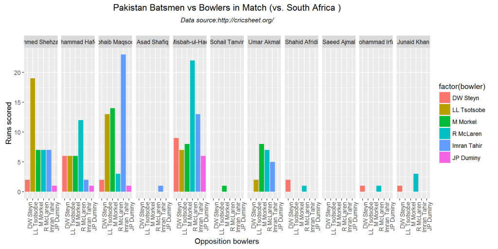
teamBatsmenVsBowlersMatch(aus_ind,'Australia',"India",plot=TRUE)

batsmenVsBowler-2

teamBatsmenVsBowlersMatch(ban_zim,'Zimbabwe',"Bangladesh", plot=TRUE)

batsmenVsBowler-3

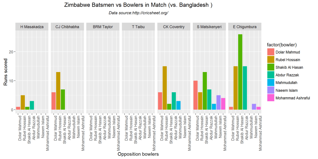
m <- teamBatsmenVsBowlersMatch(sl_wi,'West Indies',"Sri Lanka", plot=FALSE)
m
## Source: local data frame [35 x 3]
## Groups: batsman [?]
## 
##      batsman        bowler runsConceded
##       (fctr)        (fctr)        (dbl)
## 1   CH Gayle  CRD Fernando            0
## 2   DM Bravo  CRD Fernando           15
## 3   DM Bravo   NLTC Perera           21
## 4   DM Bravo    AD Mathews           10
## 5   DM Bravo    BAW Mendis           11
## 6   DM Bravo CK Kapugedera            1
## 7   DM Bravo    TM Dilshan            5
## 8   DM Bravo  HMRKB Herath           16
## 9  AB Barath   NLTC Perera            0
## 10 RR Sarwan  CRD Fernando            6
## ..       ...           ...          ...

10. Bowling Scorecard

This function provides the bowling performance, the number of overs bowled, maidens, runs conceded and wickets taken for each match

teamBowlingScorecardMatch(eng_nz,'England')
## Source: local data frame [6 x 5]
## 
##           bowler overs maidens  runs wickets
##           (fctr) (int)   (int) (dbl)   (dbl)
## 1    LE Plunkett     9       0    54       3
## 2    CT Tremlett    10       0    72       1
## 3     A Flintoff    10       0    66       0
## 4     MS Panesar    10       2    35       2
## 5  JWM Dalrymple     5       0    43       0
## 6 PD Collingwood     6       0    36       1
teamBowlingScorecardMatch(eng_nz,'New Zealand')
## Source: local data frame [6 x 5]
## 
##         bowler overs maidens  runs wickets
##         (fctr) (int)   (int) (dbl)   (dbl)
## 1 JEC Franklin     8       1    45       1
## 2      SE Bond    10       0    58       1
## 3     JDP Oram     5       0    23       0
## 4     JS Patel    10       0    53       1
## 5   DL Vettori    10       0    40       3
## 6  CD McMillan     7       1    38       2
teamBowlingScorecardMatch(aus_ind,'Australia')
## Source: local data frame [6 x 5]
## 
##         bowler overs maidens  runs wickets
##         (fctr) (int)   (int) (dbl)   (dbl)
## 1    RJ Harris    10       0    57       1
## 2     MA Starc     8       0    49       0
## 3     CJ McKay    10       1    53       3
## 4 DT Christian    10       0    45       0
## 5    DJ Hussey     3       0    13       0
## 6   XJ Doherty     9       0    51       2

11. Wicket Kind

The plots below provide the bowling kind of wicket taken by the bowler (caught, bowled, lbw etc.)

teamBowlingWicketKindMatch(aus_ind,"India","Australia")

bowlingWicketKind-1

teamBowlingWicketKindMatch(aus_ind,"Australia","India")

bowlingWicketKind-2

teamBowlingWicketKindMatch(pak_sa,"South Africa","Pakistan")

bowlingWicketKind-3

m <-teamBowlingWicketKindMatch(sl_wi,"Sri Lanka",plot=FALSE)
m
##           bowler wicketKind wicketPlayerOut runs
## 1   CRD Fernando     bowled        CH Gayle   45
## 2    NLTC Perera     caught       AB Barath   36
## 3   HMRKB Herath        lbw       RR Sarwan   54
## 4     BAW Mendis     caught   S Chanderpaul   46
## 5    NLTC Perera        lbw        DM Bravo   36
## 6    NLTC Perera     caught       DJG Sammy   36
## 7   CRD Fernando     caught        DJ Bravo   45
## 8     BAW Mendis     caught       NO Miller   46
## 9     BAW Mendis     caught        CS Baugh   46
## 10    BAW Mendis     caught         SJ Benn   46
## 11    AD Mathews   noWicket        noWicket   33
## 12 CK Kapugedera   noWicket        noWicket    7
## 13    TM Dilshan   noWicket        noWicket   25

12. Wicket vs Runs conceded

The plots below provide the wickets taken and the runs conceded by the bowler in the match

teamBowlingWicketRunsMatch(pak_sa,"Pakistan","South Africa")

wicketRuns-1

teamBowlingWicketRunsMatch(aus_ind,"Australia","India")

wicketRuns-2

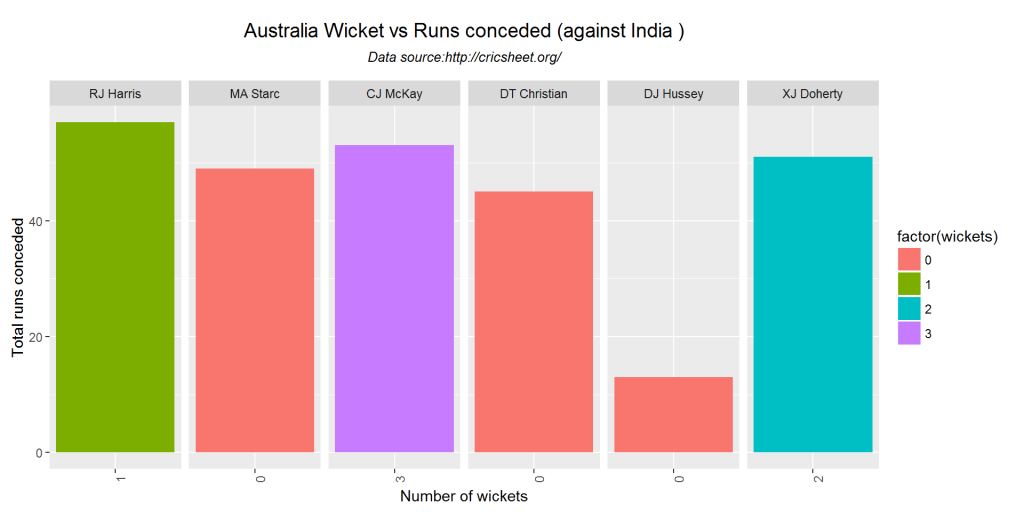
m <-teamBowlingWicketRunsMatch(sl_wi,"West Indies","Sri Lanka", plot=FALSE)
m
## Source: local data frame [6 x 5]
## 
##      bowler overs maidens  runs wickets
##      (fctr) (int)   (int) (dbl)   (chr)
## 1 R Rampaul     5       0    44       1
## 2 DJG Sammy    10       1    61       1
## 3  DJ Bravo    10       0    58       3
## 4  CH Gayle    10       0    34       0
## 5   SJ Benn    10       1    38       4
## 6 NO Miller     5       0    35       0

13. Wickets taken by bowler

The plots provide the wickets taken by the bowler

m <-teamBowlingWicketMatch(eng_nz,'England',"New Zealand", plot=FALSE)
m
##           bowler wicketKind wicketPlayerOut runs
## 1    LE Plunkett        lbw      SP Fleming   54
## 2    LE Plunkett     caught       PG Fulton   54
## 3 PD Collingwood     caught     LRPL Taylor   36
## 4     MS Panesar    stumped     CD McMillan   35
## 5    LE Plunkett     caught       L Vincent   54
## 6     MS Panesar     caught     BB McCullum   35
## 7    CT Tremlett     caught    JEC Franklin   72
## 8     A Flintoff   noWicket        noWicket   66
## 9  JWM Dalrymple   noWicket        noWicket   43
teamBowlingWicketMatch(sl_wi,"Sri Lanka","West Indies")

bowlingWickets-1

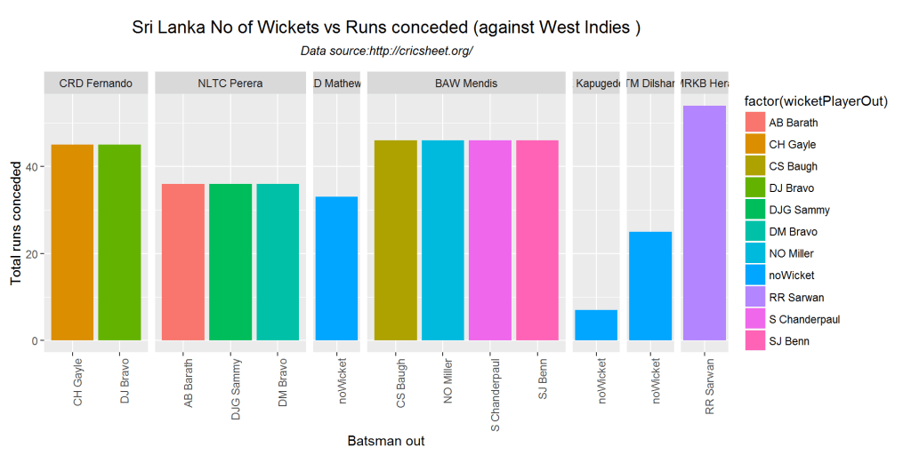
teamBowlingWicketMatch(eng_nz,"New Zealand","England")

bowlingWickets-2

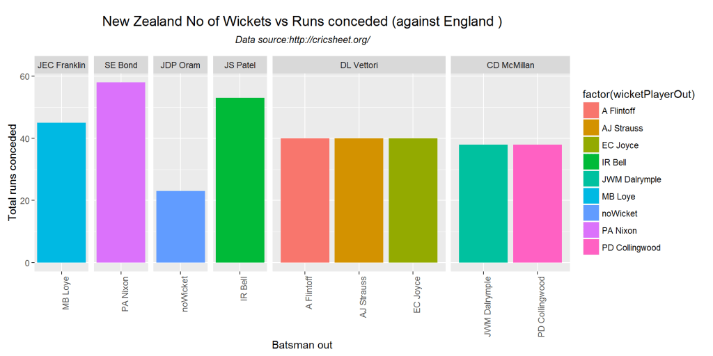
14. Bowler Vs Batsmen

The functions compute and display how the different bowlers of the country performed against the batting opposition.

teamBowlersVsBatsmenMatch(ban_zim,"Bangladesh","Zimbabwe")

bowlerVsBatsmen-1

teamBowlersVsBatsmenMatch(aus_ind,"India","Australia")

bowlerVsBatsmen-2

teamBowlersVsBatsmenMatch(eng_nz,"England","New Zealand")

bowlerVsBatsmen-3

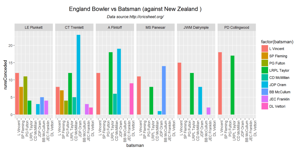
m <- teamBowlersVsBatsmenMatch(pak_sa,"Pakistan",plot=FALSE)
m
## Source: local data frame [30 x 3]
## Groups: bowler [?]
## 
##            bowler        batsman runsConceded
##            (fctr)         (fctr)        (dbl)
## 1  Mohammad Irfan      Q de Kock           25
## 2  Mohammad Irfan        HM Amla           17
## 3  Mohammad Irfan   F du Plessis            0
## 4  Mohammad Irfan AB de Villiers            9
## 5   Sohail Tanvir      Q de Kock           11
## 6   Sohail Tanvir        HM Amla            6
## 7   Sohail Tanvir      JP Duminy            9
## 8   Sohail Tanvir      R McLaren           12
## 9     Junaid Khan      Q de Kock           24
## 10    Junaid Khan        HM Amla            6
## ..            ...            ...          ...

15. Match worm graph

The plots below provide the match worm graph for the matches

matchWormGraph(aus_ind,'Australia',"India")

matchWorm-1

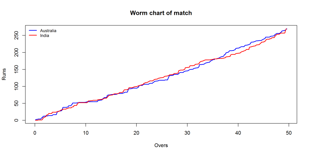
matchWormGraph(sl_wi,'Sri Lanka',"West Indies")
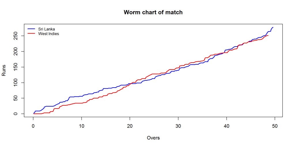
matchWorm-2

Conclusion

This post included all functions between 2 opposing countries from the package yorkr.As mentioned above the yaml match files have been already converted to dataframes and are available for download from Github. Go ahead and give it a try

To be continued. Watch this space!

Important note: Do check out my other posts using yorkr at yorkr-posts

You may also like

The making of cricket package yorkr – Part 3

Introduction

This is the 3rd part of my cricket package yorkr in R. In my 2 earlier posts

  1. The making of cricket package yorkr – Part 1. This post analyzed the performance of team in a ODI match. The batting and bowling performances of the team were analyzed. This post also performed analyses of a country in all matches against another country for e.g. India vs All matches agianst Australia. The best performers with the bat and ball were determined, the best batting partnerships, the performances at different venues etc. The detailed performances of the bowlers of India and Australia in the confrontation were also analyzed.
  2. The making of cricket package yorkr – Part 2 This post includes all ODI matches between a country and others. For obvious reasons I have chosen India and selected all ODI matches played by India with other countries. This included batting and bowling performances of the country against all oppositions.

As mentioned in my earlier posts the data is taken from Cricsheet

If you are passionate about cricket, and love analyzing cricket performances, then check out my 2 racy books on cricket! In my books, I perform detailed yet compact analysis of performances of both batsmen, bowlers besides evaluating team & match performances in Tests , ODIs, T20s & IPL. You can buy my books on cricket from Amazon at $12.99 for the paperback and $4.99/$6.99 respectively for the kindle versions. The books can be accessed at Cricket analytics with cricketr  and Beaten by sheer pace-Cricket analytics with yorkr  A must read for any cricket lover! Check it out!!

1

s), and $4.99/Rs 320 and $6.99/Rs448 respectively

Important note: Do check out my other posts using yorkr at yorkr-posts

Important note: Do check out all the posts on the python avatar of yorkr, namely ‘yorkpy’ in my post ‘Pitching yorkpy … short of good length to IPL – Part 1

In this post I look at individual performances of batsmen and bowlers in ODIs. For this post I have chosen Virat Kohli & Mahendra Singh Dhoni from India. Kohli has been consistent and in great form right through. Dhoni follows Kohli very closely in ODIs. Dhoni besides his shrewd captaincy is one of the best ODI batsman and a great finisher. I have include AB Devilliers from South Africa who seems to invent new strokes and shots every time, much like Glenn Maxwell.

For bowling analyses I have selected RA Jadeja, Harbhajan Singh *the top Indian ODI bowlers) and Mitchell Johnson who is among the best in the world.

This post is also available at RPubs at yorkr-3. You can also download this post as a pdf from yorkr-3.pdf

Checkout my interactive Shiny apps GooglyPlus (plots & tables) and Googly (only plots) which can be used to analyze IPL players, teams and matches.

My earlier package ‘cricketr’ (see Introducing cricketr: An R package for analyzing performances of cricketers) was based on data from ESPN Cricinfo Statsguru. If you want to take a look at my book with all my articles based on my package cricketr at – Cricket analytics with cricketr!!!. The book is also available in paperback and kindle versions at Amazon which has, by the way, better formatting!

I have added some quick observations on the plots below. However there is a lot more that can be discerned from the plots that I can possibly explain. The charts do display a wealth of insights. Do take a close look at the plots.

library(dplyr)
library(ggplot2)
library(yorkr)
library(reshape2)
library(gridExtra)
library(rpart.plot)

1. Batting Details

The following functions get the overall batting details for a country against all opposition.

a <- getTeamBattingDetails("India",save=TRUE)
b <- getTeamBattingDetails("South Africa",save=TRUE)

2. Get Batsman details

Now I get the details of the batsmen Virat Kohli and Mahendra Singh Dhoni from the saved India file and AB De Villiers from the saved South Africa file

kohli <- getBatsmanDetails(team="India",name="Kohli")
dhoni <- getBatsmanDetails(team="India",name="Dhoni")
devilliers <-  getBatsmanDetails(team="South Africa",name="Villiers")

3. Display the dataframe

the dataframe obtained from the calls above provide detailed information for the batsman in every ODI match. This dataframe has all the fields that can be obtained from ESPN Cricinfo

Untitled


Performance analyses of batsmen


4. Runs vs deliveries plot

It can be seen from the plots below that Kohli is very consistent in the runs scored. The runs crowd near the regression curve. There is more variance in Dhoni and De Villiers performance. The band on either side of the regression curve represents the 95% confidence interval(A 95% confidence level means that 95% of the intervals would include the population parameter).

p1 <-batsmanRunsVsDeliveries(kohli,"Kohli")
p2 <- batsmanRunsVsDeliveries(dhoni, "Dhoni")
p3 <- batsmanRunsVsDeliveries(devilliers,"De Villiers")
grid.arrange(p1,p2,p3, ncol=3)

runsDel-1

5. Total runs vs 4s vs 6s plot

The plots below show the runs (Total runs, Runs from 4s & Runs from sixes) vs the deliveries faced. Kohli scores more runs and more fours which can be evaluated from the slope of the blue and red regression lines (reaches 150+,50+) for Total runs and Runs from fours). De Villers has more Runs from sixes as can be seen the 3rd sub plot (green line)

kohli46 <- select(kohli,batsman,ballsPlayed,fours,sixes,runs)
p1 <- batsmanFoursSixes(kohli46,"Kohli")
dhoni46 <- select(dhoni,batsman,ballsPlayed,fours,sixes,runs)
p2 <- batsmanFoursSixes(dhoni46,"Dhoni")
devilliers46 <- select(devilliers,batsman,ballsPlayed,fours,sixes,runs)
p3 <- batsmanFoursSixes(devilliers46, "De Villiers")
grid.arrange(p1,p2,p3, ncol=3)

4s6s-1

6. Batsmen dismissals

Interestingly it can be seen that Dhoni has remained unbeaten more often (47 times) than Kohli or De Villiers. Dhoni despite being a great runner between wickets has been run-out more often.

p1 <-batsmanDismissals(kohli,"Kohli")
p2 <- batsmanDismissals(dhoni, "Dhoni")
p3 <- batsmanDismissals(devilliers, "De Villiers")
grid.arrange(p1,p2,p3, ncol=3)

dismissal-1

7. Batsmen Strike Rate

From the plot below Kohli has the best strike rate till 100 runs, the slope seems to steeper. De Villiers seems to do better after 100 runs.

p1 <-batsmanMeanStrikeRate(kohli,"Kohli")
p2 <- batsmanMeanStrikeRate(dhoni, "Dhoni")
p3 <- batsmanMeanStrikeRate(devilliers, "De Villiers")
grid.arrange(p1,p2,p3, ncol=3)

meanSR-1

8. Batsmen moving average

Kohli’s and De Villiers’ form can be seen to be improving over the years. Dhoni seems to have hit a slump in recent times. But we have to keep in mind that he has the second highest ODI runs in India and is just behind Kohli

p1 <-batsmanMovingAverage(kohli,"Kohli")
p2 <- batsmanMovingAverage(dhoni, "Dhoni")
p3 <- batsmanMovingAverage(devilliers, "De Villiers")
grid.arrange(p1,p2,p3, ncol=3)

bmanMA-1

9. Batsmen against opposition

Kohli averages 50 runs against 6 countries, to Dhoni’s 4. Kohli performs well against Australia, New Zealand, West Indies,Pakistan,Bangladesh. Kohli’s performance against England has been mediocre. De Villiers averages around 50 with 5 countries

batsmanRunsAgainstOpposition(kohli,"Kohli")

bmanOppn-1

batsmanRunsAgainstOpposition(dhoni, "Dhoni")

bmanOppn-2

batsmanRunsAgainstOpposition(devilliers, "De Villiers")

bmanOppn-3

10. Batsmen runs at different venues

Kohli’s favorite hunting grounds in ODI are Adelaide, Sydney, Western Australia, Wankhede. Dhoni’s best performances are at Lords, Sydney,Chepauk.

batsmanRunsVenue(kohli,"Kohli")

bmanOppn1-1

batsmanRunsVenue(dhoni, "Dhoni")

bmanOppn1-2

batsmanRunsVenue(devilliers, "De Villiers")

bmanOppn1-3

11. Batsmen runs predict

The plots below predict the number of deliveries needed by each batsmen to score runs shown. For this I have used classification trees based on deliveries and runs using the package rpart. From the plot for Kohli it can be seen that for 58 deliveries scores around 52 runs. On the other hand De Villiers needs just over 40 deliveries to score 52 runs.

par(mfrow=c(1,3))
par(mar=c(4,4,2,2))
batsmanRunsPredict(kohli,"Kohli")
batsmanRunsPredict(dhoni, "Dhoni")
batsmanRunsPredict(devilliers, "De Villiers")

runsPred-1

dev.off()
## null device 
##           1

12. Get team bowling details

The function below all the ODI matches between India or Australia and all other countries

c <- getTeamBowlingDetails("India",save=TRUE)
d <- getTeamBowlingDetails("Australia",save=TRUE)

13. Get wicket details

The functions below gets the data frame for each bowler

jadeja <- getBowlerWicketDetails(team="India",name="Jadeja")
harbhajan <- getBowlerWicketDetails(team="India",name="Harbhajan")
ashwin <- getBowlerWicketDetails(team="India",name="Ashwin")
johnson <-  getBowlerWicketDetails(team="Australia",name="Johnson")

14. Display data frame

The details of the data frame is shown below

knitr::kable(head(jadeja))
bowler overs maidens runs wickets economyRate date opposition venue
RA Jadeja 6 0 40 0 6.67 2009-02-08 Sri Lanka R Premadasa Stadium
RA Jadeja 7 1 34 0 4.86 2009-06-26 West Indies Sabina Park, Kingston
RA Jadeja 2 0 12 0 6.00 2009-06-28 West Indies Sabina Park, Kingston
RA Jadeja 9 0 39 1 4.33 2009-10-25 Australia Reliance Stadium
RA Jadeja 7 1 35 4 5.00 2009-10-28 Australia Vidarbha Cricket Association Stadium, Jamtha

15. Bowler Economy rate

Harbhajan and Ashwin have a better economy rate than RA Jadeja

p1 <- bowlerEconomyRate(jadeja,"RA Jadeja")
p2<-bowlerEconomyRate(harbhajan, "Harbhajan")
p3<-bowlerEconomyRate(ashwin, "Ashwin")
p4<-bowlerEconomyRate(johnson, "MG Johnson")
grid.arrange(p1,p2,p3,p4, ncol=2)

ER-1

15. Mean runs conceded by bowler

p1<-bowlerMeanRuns(jadeja,"RA Jadeja")
p2<-bowlerMeanRuns(harbhajan, "Harbhajan")
p3<-bowlerMeanRuns(ashwin, "Ashwin")
p4<-bowlerMeanRuns(johnson, "MG Johnson")
grid.arrange(p1,p2,p3,p4, ncol=2)

meanRuns-1

15. Moving average of bowler

From the plots below MG Johnson, Harbhajan and Ashwin have been performing very consistently. RA Jadeja bowling seems to be taking a nosedive, though he is at the top of all ODI bowlers of India

p1<-bowlerMovingAverage(jadeja,"RA Jadeja")
p2<-bowlerMovingAverage(harbhajan, "Harbhajan")
p3<-bowlerMovingAverage(ashwin, "Ashwin")
p4<-bowlerMovingAverage(johnson, "MG Johnson")
grid.arrange(p1,p2,p3,p4, ncol=2)

bwlrMA-1

16. Wicket average

Jadeja has a better wicket average than Harbhajan and Ashwin.Jadeja and Ashwin average around 2 wickets Harbhajan averages 1.5 wickets(tendency to 2)

p1<-bowlerWicketPlot(jadeja,"RA Jadeja")
p2<-bowlerWicketPlot(harbhajan, "Harbhajan")
p3<-bowlerWicketPlot(ashwin, "Ashwin")
p4<-bowlerWicketPlot(johnson, "MG Johnson")
grid.arrange(p1,p2,p3,p4, ncol=2)

bwlrWkt-1

16. Wickets opposition

Jadeja’s best performances have been against England, Pakistan, New Zealand and Zimbabwe. For Harbhajan it has been New Zealand, Sri Lanka and Zimbabwe.

bowlerWicketsAgainstOpposition(jadeja,"RA Jadeja")

bwlrOppn-1

bowlerWicketsAgainstOpposition(harbhajan, "Harbhajan")

bwlrOppn-2

bowlerWicketsAgainstOpposition(ashwin, "Ashwin")

bwlrOppn-3

bowlerWicketsAgainstOpposition(johnson, "MG Johnson")

bwlrOppn-4

16. Wickets venue

The top 20 venues for each bowler is shown in the plots

bowlerWicketsVenue(jadeja,"RA Jadeja")

bwlrVenue-1

bowlerWicketsVenue(harbhajan, "Harbhajan")

bwlrVenue-2

bowlerWicketsVenue(ashwin, "Ashwin")

bwlrVenue-3

bowlerWicketsVenue(johnson, "MG Johnson")

bwlrVenue-4

16. Create a data frame with wickets and deliveries

jadeja1 <- getDeliveryWickets(team="India",name="Jadeja",save=FALSE)
harbhajan1 <- getDeliveryWickets(team="India",name="Harbhajan",save=FALSE)
ashwin1 <- getDeliveryWickets(team="India",name="Ashwin",save=FALSE)
johnson1 <- getDeliveryWickets(team="Australia",name="MG Johnson",save=FALSE)

17. Deliveries to wickets plots

The following plots try to predict the average number of deliveries required for the wickets taken. As in the batsman runs predict I have used classification trees between deliverie at which a wicket was taken. The package rpart was used for the classification. The internediate nodes are the number of deliveries and the leaf nodes are the wickets taken. Though the wickets are in decimal we can intepret the tree as follows For RA Jadeja 22 to take 1.6 wicket (~2 wickets). Interestingly Harbhajan needs

par(mfrow=c(1,2))
par(mar=c(4,4,2,2))
bowlerWktsPredict(jadeja1,"RA Jadeja")
bowlerWktsPredict(harbhajan1,"Harbhajan Sigh")

wktPrd1-1

dev.off()
## null device 
##           1

Similarly MG Johnson can provide a breakthrough with just around 14 deliveries

par(mfrow=c(1,2))
par(mar=c(4,4,2,2))
bowlerWktsPredict(ashwin1,"Ravichander Ashwin")
bowlerWktsPredict(johnson1,"MG Johnson")

wktPred2-1

dev.off()
## null device 
##           1

Conclusion

ODI batsman

  1. The top 2 ODI Indian batsman(Kohli and Dhoni) and De Villiers of South Africa were considered.
  2. Kohli has a better strike rate till about 100 runs(steeper slope) and De Villiers beyond 100.
  3. Dhoni has remained unbeaten more number of times than the other 2. It may have been possible that his average would have been higher if he had come in earlier
  4. Kohli and De Villiers have performed consistently. Dhoni needs to get back his touch

ODI bowlers

  1. RA Jadeja has a better wicket taking rate than Harbhajan and Ashwin.
  2. Ashwin and Harbhajan have a better economy rate than Jadeja
  3. Harbhjanan, Ashwin and MG Johnson have performed consistently while RA Jadeja’s performance has been on the decline.
  4. Harbhajan and MG Johnson need around 11 balls to make a break through

This was probably the last set of functions for my cricket package yorkr. Over the next several weeks I will be cleaning up, documenting, refining the functions and removing any glitches. I hope to have the package released in the next 6-8 weeks

Also see

  1. Cricket analytics with cricketr
  2. Sixer: An R package cricketr’s new Shiny avatar

You may also like

  1. What’s up Watson? Using IBM Watson’s QAAPI with Bluemix, NodeExpress
  2. The common alphabet of programming languages
  3. A method to crowd source pothole marking on (Indian) roads
  4. The Anomaly
  5. Simulating the domino effect in Android using Box2D and AndEngine
  6. Presentation on Wireless Technologies – Part 1
  7. Natural selection of database technology through the years

Cricket analytics with cricketr in paperback and Kindle versions

Untitled

My book “Cricket analytics with cricketr” is now available in paperback and Kindle versions. The paperback is available from Amazon (US, UK and Europe) for $ 48.99. The Kindle version can be downloaded from the Kindle store for $2.50 (Rs 169/-). Do pick your copy. It should be a good read for a Sunday afternoon.

This book of mine contains my posts based on my R package ‘cricketr’ now in CRAN. The package cricketr can analyze both batsmen and bowlers for all formats of the game Test, ODI and Twenty20. The package uses the data from ESPN Cricinfo. The analyses include runs frequency charts, performances of batsmen and bowlers in different grounds and against different teams, moving  average of  runs/wickets over the career, mean strike rate, mean economy rate and so on.

The book includes the following chapters based on my R package cricketr  There are 2 additional articles where I use Machine Learning with the package Octave.

CONTENTS
Cricket Analytics with cricketr 11
1.1. Introducing cricketr! : An R package to analyze performances of cricketers 11
1.2. Taking cricketr for a spin – Part 1 49
1.2. cricketr digs the Ashes! 70
1.3. cricketr plays the ODIs! 99
1.4. cricketr adapts to the Twenty20 International! 141
1.5. Sixer – R package cricketr’s new Shiny avatar 170
2. Other cricket posts in R 180
2.1. Analyzing cricket’s batting legends – Through the mirage with R 180
2.2. Mirror, mirror … the best batsman of them all? 206
3. Appendix 220
Cricket analysis with Machine Learning using Octave 220
3.1. Informed choices through Machine Learning – Analyzing Kohli, Tendulkar and Dravid 221
3.2. Informed choices through Machine Learning-2 Pitting together Kumble, Kapil, Chandra 234
Further reading 248
Important Links 249

You can download the latest PDF version of the book  at  ‘Cricket analytics with cricketr and cricpy: Analytics harmony with R and Python-6th edition

I do hope you have a great time reading it. Do pick up your copy. Feel free to get in touch with me with your comments and suggestions.  I have more interesting things lined up for the future.

Watch this space!

You may also like
1. Literacy in India : A deepR dive.
2. Natural Language Processing: What would Shakespeare say?
3. Revisiting crimes against women in India
4. Experiments with deblurring using OpenCV
5. TWS-4: Gossip protocol: Epidemics and rumors to the rescue
6. Bend it like Bluemix, MongoDB with autoscaling – Part 1
7. “Is it animal? Is it an insect?” in Android

Cricket analytics with cricketr!!!

Important note: The 3rd paperback & kindle editions of my books on Cricket, now on Amazon
cricket

My ebook “Cricket analytics with cricketr’  has been published in Leanpub.  You can now download the book (hot off the press!)  for all formats to your favorite device (mobile, iPad, tablet, Kindle)  from the Leanpub  “Cricket analytics with cricketr”. The book has been published in the following formats namely

  • PDF (for your computer)
  • EPUB (for iPad or tablets. Save the file cricketr.epub to Google Drive/Dropbox and choose “Open in” iBooks for iPad)
  • MOBI (for Kindle. For this format, I suggest that you download & install SendToKindle for PC/Mac. You can then right click the downloaded cricketr.mobi and choose SendToKindle. You will need to login to your Kindle account)

From Leanpub
UntitledLeanpub uses a variable pricing model. I have priced the book attractively (I think!)  at $2.50 with a minimum price of $0.00 (FREE!!! limited time offer!).  The link is “Cricket analytics with cricketr

This format works with all type Kindle, Android tablet, iPad.

From Amazon

If you are passionate about cricket, and love analyzing cricket performances, then check out my 2 racy books on cricket! In my books, I perform detailed yet compact analysis of performances of both batsmen, bowlers besides evaluating team & match performances in Tests , ODIs, T20s & IPL. You can buy my books on cricket from Amazon at $12.99 for the paperback and $4.99/$6.99 respectively for the kindle versions. The books can be accessed at Cricket analytics with cricketr  and Beaten by sheer pace-Cricket analytics with yorkr  A must read for any cricket lover! Check it out!!

You can download the latest PDF version of the book  at  ‘Cricket analytics with cricketr and cricpy: Analytics harmony with R and Python-6th edition

1

Important note: The latest release of ‘cricketr’ now includes the ability to analyze performances of teams now!!  See Cricketr adds team analytics to its repertoire!!!

Preface
Cricket has been the “national passion” of India for decades. As a boy I was also held in thrall by a strong cricketing passion like many. Cricket is a truly fascinating game! I would catch the sporting action with my friends as we crowded around a transistor that brought us live, breathless radio commentary. We also spent many hours glued to live cricket action on the early black and white TVs. This used to be an experience of sorts, as every now and then a part of the body of the players, would detach itself and stretch to the sides. But it was enjoyable all the same.

Nowadays broadcast technology has improved so much and we get detailed visual analysis of the how each bowler varies the swing and length of the delivery. We are also able to see the strokes of batsman in slow motion.   Similarly computing technology has also advanced by leaps and bounds and we can analyze players in great detail with a few lines of code in languages like R, Python etc.

In 2015, I completed Machine Learning from Stanford at Coursera.  I was looking around for data to play around with, when it suddenly struck me that I could do some regression analysis of batting records.  In the subsequent months, I took the Data Science Specialization from John Hopkins University, which triggered more ideas in me. One thing led to another and I managed to put together an R package called ‘cricketr’.  I developed this package over 7 months adding and refining functions. Finally, I managed to submit the package to CRAN.  During the development of the package for different formats of the game I wrote a series of posts in my blog.

This book is a collection of those cricket related posts.  There are 6 posts based on my R package cricketr. I have also included 2 earlier posts based on R which I wrote before I created my R package. Finally, I also include another 2 cricket posts based on Machine Learning in which I used the language Octave.

My cricketr’ package is a first, for cricket analytics, howzzat!  and I am certain that it won’t be the last. Cricket is a wonderful pitch for statisticians, data scientists and machine learning experts. So you can expect some cool packages in the years to come.

I had a great time developing the package. I hope you have a wonderful time reading this book. Do remember to download from “Cricket analytics with cricketr

Feel free to get in touch with me anytime through email included below

Tinniam V Ganesh
tvganesh.85@gmail.com
January 28, 2016

Sixer – R package cricketr’s new Shiny avatar

Published in R-bloggers: Sixer – R package cricketr’s new Shiny app

In this post I create a Shiny App, Sixer, based on my R package cricketr. I had developed the R package cricketr, a few months back for analyzing the performances of batsman and bowlers in all formats of the game (Test, ODI and Twenty 20). This package uses the statistics info available in ESPN Cricinfo Statsguru. I had written a series of posts using the cricketr package where I chose a few batsmen, bowlers and compared their performances of these players. Here I have created a complete Shiny app with a lot more players and with almost all the features of the cricketr package. The motivation for creating the Shiny app was to

  • To show case the  ‘cricketr’ package and to highlight its functionalities
  • Perform analysis of more batsman and bowlers
  • Allow users to interact with the package and to allow them to try out the different features and functions of the package and to also check performances of some of their favorite crickets

If you are passionate about cricket, and love analyzing cricket performances, then check out my racy book on cricket ‘Cricket analytics with cricketr and cricpy – Analytics harmony with R & Python’! This book discusses and shows how to use my R package ‘cricketr’ and my Python package ‘cricpy’ to analyze batsmen and bowlers in all formats of the game (Test, ODI and T20). The paperback is available on Amazon at $21.99 and  the kindle version at $9.99/Rs 449/-. A must read for any cricket lover! Check it out!!

Untitled


$4.99/Rs 320 and $6.99/Rs448 respectively

Important note 1: The latest release of ‘cricketr’ now includes the ability to analyze performances of teams now!!  See Cricketr adds team analytics to its repertoire!!!

Important note 2 : Cricketr can now do a more fine-grained analysis of players, see Cricketr learns new tricks : Performs fine-grained analysis of players

Important note 3: Do check out the python avatar of cricketr, ‘cricpy’ in my post ‘Introducing cricpy:A python package to analyze performances of cricketers

a) You can try out the interactive  Shiny app Sixer at – Sixer
b) The code for this Shiny app project can be cloned/forked from GitHub – Sixer
Note: Please be mindful of  ESPN Cricinfo Terms of Use.
(Take a look at my short video tutorial on my R package cricketr on Youtube – R package cricketr – A short tutorial)

Important note: Do check out my other posts using cricketr at cricketr-posts

In this Shiny app I have 5 tabs which perform the following function
1.  Analyze Batsman
This tab analyzes batsmen based on different functions and plots the performances of the selected batsman. There are functions that compute and display batsman’s run-frequency ranges, Mean Strike rate, No of 4’s, dismissals, 3-D plot of Runs scored vs Balls Faced and Minutes at crease, Contribution to wins & losses, Home-Away record etc. The analyses can be done for Test cricketers, ODI and Twenty 20 batsman. I have included most of the Test batting giants including Tendulkar, Dravid, Sir Don Bradman, Viv Richards, Lara, Ponting etc. Similarly the ODI list includes Sehwag, Devilliers, Afridi, Maxwell etc. The Twenty20 list includes the Top 10 Twenty20 batsman based on their ICC rankings

2. Analyze bowler
This tab analyzes the bowling performances of bowlers, Wickets percentages, Mean Economy Rate, Wickets at different venues, Moving average of wickets etc. As earlier I have all the Top bowlers including Warne, Muralidharan, Kumble- the famed Indian spin quartet of Bedi, Chandrasekhar, Prasanna, Venkatraghavan, the deadly West Indies trio of Marshal, Roberts and Holding and the lethal combination of Imran Khan, Wasim Akram and Waqar Younis besides the dangerous Dennis Lillee and Jeff Thomson. Do give the functions a try and see for yourself the performances of these individual bowlers

3. Relative performances of batsman
This tab allows the selection of multiple batsmen (Test, ODI and Twenty 20) for comparisons. There are 2 main functions Relative Runs Frequency performance and Relative Mean Strike Rate

4. Relative performances of bowlers
Here we can compare bowling performances of multiple bowlers, which include functions Relative Bowling Performance and Relative Economy Rate. This can be done for Test, ODI and Twenty20 formats

5. Check for In-Form status of players
This tab checks the form status of batsman or bowler selected for all of the different formats of the game. The below computation uses Null Hypothesis testing and p-value to determine if the batsman is in-form or out-of-form. For this 90% of the career runs is chosen as the population and the mean computed. The last 10% is chosen to be the sample set and the sample Mean and the sample Standard Deviation are calculated. Note: The accuracy of the p-value test depends on the size of the population and the size of the sample set. It  may not be very significant for players with a few innings played.

Some of my earlier posts based my R package cricketr are listed below
1. Introducing cricketr!: An R package for analyzing performances of cricketers
2. Taking cricketr for a spin – Part 1
3. cricketr plays the ODIs
4. cricketr adapts to the Twenty20 International
5. cricketr digs the Ashes

Do try out the interactive Sixer Shiny app – Sixer
You can clone the code from Github – Sixer

There is not much in way of explanation. The Shiny app’s use is self-explanatory. You can choose a match type ( Test,ODI or Twenty20), choose a batsman/bowler  from the drop down list and select the plot you would like to seeHere a few sample plots
A. Analyze batsman tab
i) Batsman – Brian Lara , Match Type – Test, Function – Mean Strike Rate
sxr-1ii) Batsman – Shahid Afridi, Match Type –  ODI, Function – Runs vs Balls faced
The plot below shows that if Afridi faces around 50 balls he is likely to score around 60 runs in ODIs.
sxr-2iii)   Batsman – Chris Gayle, Match Type – Twenty20  Function – Moving Average
sxr-3B. Analyze bowler tab

i. Bowler – B S Chandrasekhar, Match Type – Test, Function – Wickets vs Runs
sxr-4ii)  Bowler – Malcolm Marshall, Match Type – Test, Function – Mean Economy Ratesxr-5iii)  Bowler – Sunil Narine, Match Type – Twenty 20, Function – Bowler Wicket Rate
sxr-6
C. Relative performance of batsman (you can select more than 1)
The below plot gives the Mean Strike Rate of batsman. Viv Richards, Brian Lara, Sanath Jayasuriya and David Warner are best strikers of the ball.
sxr-7

Here are some of the great strikers of the ball in ODIs
sxr-8D. Relative performance of bowlers (you can select more than 1)
Finally a look at the famed Indian spin quartet.  From the plot below it can be seen that  B S Bedi  & Venkatraghavan were more economical than Chandrasekhar and Prasanna.
sxr-9

But the latter have a better 4-5 wicket haul than the former two as seen in the plot below

sxr-11Finally a look at the average number of balls to take a wicket by the Top 4 Twenty 20 bowlers.
sxr-10

E. Check for In-form status of players
Note: The accuracy of the p-value depends on the size of the population and the size of the sample set. It  may not be very significant for smaller data sizes

i. Match Type – Test,  Player Type – Batsman  Name – Wickets v
In this plot the in-form status of Viv Richards is checked. This shows that Viv Richards was out-of-form
sxr-12In the plot below the form status of S. Venkataraghavan is shown. According to this at the time of  his retirement S Venkat was still in-form
sxr-13

Do give the Shiny app Sixer a try.

Also see
1. Literacy in India : A deepR dive.
2.  Natural Language Processing: What would Shakespeare say?
3. Revisiting crimes against women in India
4. Informed choices through Machine Learning : Analyzing Kohli, Tendulkar and Dravid
5. Experiments with deblurring using OpenCV
6.  What’s up Watson? Using IBM Watson’s QAAPI with Bluemix, NodeExpress – Part 1
7.  Working with Node.js and PostgreSQL
8. A method for optimal bandwidth usage by auctioning available bandwidth using the OpenFlow Protocol
9.  Latency, throughput implications for the cloud
10.  A closer look at “Robot horse on a Trot! in Android”

cricketr plays the ODIs!

Published in R bloggers: cricketr plays the ODIs

Introduction

In this post my package ‘cricketr’ takes a swing at One Day Internationals(ODIs). Like test batsman who adapt to ODIs with some innovative strokes, the cricketr package has some additional functions and some modified functions to handle the high strike and economy rates in ODIs. As before I have chosen my top 4 ODI batsmen and top 4 ODI bowlers.

Unititled2

If you are passionate about cricket, and love analyzing cricket performances, then check out my racy book on cricket ‘Cricket analytics with cricketr and cricpy – Analytics harmony with R & Python’! This book discusses and shows how to use my R package ‘cricketr’ and my Python package ‘cricpy’ to analyze batsmen and bowlers in all formats of the game (Test, ODI and T20). The paperback is available on Amazon at $21.99 and  the kindle version at $9.99/Rs 449/-. A must read for any cricket lover! Check it out!!

You can download the latest PDF version of the book  at  ‘Cricket analytics with cricketr and cricpy: Analytics harmony with R and Python-6th edition

Untitled

Important note 1: The latest release of ‘cricketr’ now includes the ability to analyze performances of teams now!!  See Cricketr adds team analytics to its repertoire!!!

Important note 2 : Cricketr can now do a more fine-grained analysis of players, see Cricketr learns new tricks : Performs fine-grained analysis of players

Important note 3: Do check out the python avatar of cricketr, ‘cricpy’ in my post ‘Introducing cricpy:A python package to analyze performances of cricketers

Do check out my interactive Shiny app implementation using the cricketr package – Sixer – R package cricketr’s new Shiny avatar

You can also read this post at Rpubs as odi-cricketr. Dowload this report as a PDF file from odi-cricketr.pdf

Important note: Do check out my other posts using cricketr at cricketr-posts

Note: If you would like to do a similar analysis for a different set of batsman and bowlers, you can clone/download my skeleton cricketr template from Github (which is the R Markdown file I have used for the analysis below). You will only need to make appropriate changes for the players you are interested in. Just a familiarity with R and R Markdown only is needed.
Batsmen

  1. Virendar Sehwag (Ind)
  2. AB Devilliers (SA)
  3. Chris Gayle (WI)
  4. Glenn Maxwell (Aus)

Bowlers

  1. Mitchell Johnson (Aus)
  2. Lasith Malinga (SL)
  3. Dale Steyn (SA)
  4. Tim Southee (NZ)

I have sprinkled the plots with a few of my comments. Feel free to draw your conclusions! The analysis is included below

The profile for Virender Sehwag is 35263. This can be used to get the ODI data for Sehwag. For a batsman the type should be “batting” and for a bowler the type should be “bowling” and the function is getPlayerDataOD()

The package can be installed directly from CRAN

if (!require("cricketr")){ 
    install.packages("cricketr",lib = "c:/test") 
} 
library(cricketr)

or from Github

library(devtools)
install_github("tvganesh/cricketr")
library(cricketr)

The One day data for a particular player can be obtained with the getPlayerDataOD() function. To do you will need to go to ESPN CricInfo Player and type in the name of the player for e.g Virendar Sehwag, etc. This will bring up a page which have the profile number for the player e.g. for Virendar Sehwag this would be http://www.espncricinfo.com/india/content/player/35263.html. Hence, Sehwag’s profile is 35263. This can be used to get the data for Virat Sehwag as shown below

sehwag <- getPlayerDataOD(35263,dir="..",file="sehwag.csv",type="batting")

Analyses of Batsmen

The following plots gives the analysis of the 4 ODI batsmen

  1. Virendar Sehwag (Ind) – Innings – 245, Runs = 8586, Average=35.05, Strike Rate= 104.33
  2. AB Devilliers (SA) – Innings – 179, Runs= 7941, Average=53.65, Strike Rate= 99.12
  3. Chris Gayle (WI) – Innings – 264, Runs= 9221, Average=37.65, Strike Rate= 85.11
  4. Glenn Maxwell (Aus) – Innings – 45, Runs= 1367, Average=35.02, Strike Rate= 126.69

Plot of 4s, 6s and the scoring rate in ODIs

The 3 charts below give the number of

  1. 4s vs Runs scored
  2. 6s vs Runs scored
  3. Balls faced vs Runs scored

A regression line is fitted in each of these plots for each of the ODI batsmen A. Virender Sehwag

par(mfrow=c(1,3))
par(mar=c(4,4,2,2))
batsman4s("./sehwag.csv","Sehwag")
batsman6s("./sehwag.csv","Sehwag")
batsmanScoringRateODTT("./sehwag.csv","Sehwag")

sehwag-4s6sSR-1

dev.off()
## null device 
##           1

B. AB Devilliers

par(mfrow=c(1,3))
par(mar=c(4,4,2,2))
batsman4s("./devilliers.csv","Devillier")
batsman6s("./devilliers.csv","Devillier")
batsmanScoringRateODTT("./devilliers.csv","Devillier")

devillier-4s6SR-1

dev.off()
## null device 
##           1

C. Chris Gayle

par(mfrow=c(1,3))
par(mar=c(4,4,2,2))
batsman4s("./gayle.csv","Gayle")
batsman6s("./gayle.csv","Gayle")
batsmanScoringRateODTT("./gayle.csv","Gayle")

gayle-4s6sSR-1

dev.off()
## null device 
##           1

D. Glenn Maxwell

par(mfrow=c(1,3))
par(mar=c(4,4,2,2))
batsman4s("./maxwell.csv","Maxwell")
batsman6s("./maxwell.csv","Maxwell")
batsmanScoringRateODTT("./maxwell.csv","Maxwell")

maxwell-4s6sout-1

dev.off()
## null device 
##           1

Relative Mean Strike Rate

In this first plot I plot the Mean Strike Rate of the batsmen. It can be seen that Maxwell has a awesome strike rate in ODIs. However we need to keep in mind that Maxwell has relatively much fewer (only 45 innings) innings. He is followed by Sehwag who(most innings- 245) also has an excellent strike rate till 100 runs and then we have Devilliers who roars ahead. This is also seen in the overall strike rate in above

par(mar=c(4,4,2,2))
frames <- list("./sehwag.csv","./devilliers.csv","gayle.csv","maxwell.csv")
names <- list("Sehwag","Devilliers","Gayle","Maxwell")
relativeBatsmanSRODTT(frames,names)

plot-1-1

Relative Runs Frequency Percentage

Sehwag leads in the percentage of runs in 10 run ranges upto 50 runs. Maxwell and Devilliers lead in 55-66 & 66-85 respectively.

frames <- list("./sehwag.csv","./devilliers.csv","gayle.csv","maxwell.csv")
names <- list("Sehwag","Devilliers","Gayle","Maxwell")
relativeRunsFreqPerfODTT(frames,names)

plot-2-1

Percentage of 4s,6s in the runs scored

The plot below shows the percentage of runs made by the batsmen by ways of 1s,2s,3s, 4s and 6s. It can be seen that Sehwag has the higheest percent of 4s (33.36%) in his overall runs in ODIs. Maxwell has the highest percentage of 6s (13.36%) in his ODI career. If we take the overall 4s+6s then Sehwag leads with (33.36 +5.95 = 39.31%),followed by Gayle (27.80+10.15=37.95%)

Percent 4’s,6’s in total runs scored

The plot below shows the contrib

frames <- list("./sehwag.csv","./devilliers.csv","gayle.csv","maxwell.csv")
names <- list("Sehwag","Devilliers","Gayle","Maxwell")
runs4s6s <-batsman4s6s(frames,names)

plot-46s-1

print(runs4s6s)
##                Sehwag Devilliers Gayle Maxwell
## Runs(1s,2s,3s)  60.69      67.39 62.05   62.11
## 4s              33.36      24.28 27.80   24.53
## 6s               5.95       8.32 10.15   13.36
 

Runs forecast

The forecast for the batsman is shown below.

par(mfrow=c(2,2))
par(mar=c(4,4,2,2))
batsmanPerfForecast("./sehwag.csv","Sehwag")
batsmanPerfForecast("./devilliers.csv","Devilliers")
batsmanPerfForecast("./gayle.csv","Gayle")
batsmanPerfForecast("./maxwell.csv","Maxwell")

swcr-perf-1

dev.off()
## null device 
##           1

3D plot of Runs vs Balls Faced and Minutes at Crease

The plot is a scatter plot of Runs vs Balls faced and Minutes at Crease. A prediction plane is fitted

par(mfrow=c(1,2))
par(mar=c(4,4,2,2))
battingPerf3d("./sehwag.csv","V Sehwag")
battingPerf3d("./devilliers.csv","AB Devilliers")

plot-3-1

dev.off()
## null device 
##           1
par(mfrow=c(1,2))
par(mar=c(4,4,2,2))
battingPerf3d("./gayle.csv","C Gayle")
battingPerf3d("./maxwell.csv","G Maxwell")

plot-4-1

dev.off()
## null device 
##           1

Predicting Runs given Balls Faced and Minutes at Crease

A multi-variate regression plane is fitted between Runs and Balls faced +Minutes at crease.

BF <- seq( 10, 200,length=10)
Mins <- seq(30,220,length=10)
newDF <- data.frame(BF,Mins)

sehwag <- batsmanRunsPredict("./sehwag.csv","Sehwag",newdataframe=newDF)
devilliers <- batsmanRunsPredict("./devilliers.csv","Devilliers",newdataframe=newDF)
gayle <- batsmanRunsPredict("./gayle.csv","Gayle",newdataframe=newDF)
maxwell <- batsmanRunsPredict("./maxwell.csv","Maxwell",newdataframe=newDF)

The fitted model is then used to predict the runs that the batsmen will score for a hypotheticial Balls faced and Minutes at crease. It can be seen that Maxwell sets a searing pace in the predicted runs for a given Balls Faced and Minutes at crease followed by Sehwag. But we have to keep in mind that Maxwell has only around 1/5th of the innings of Sehwag (45 to Sehwag’s 245 innings). They are followed by Devilliers and then finally Gayle

batsmen <-cbind(round(sehwag$Runs),round(devilliers$Runs),round(gayle$Runs),round(maxwell$Runs))
colnames(batsmen) <- c("Sehwag","Devilliers","Gayle","Maxwell")
newDF <- data.frame(round(newDF$BF),round(newDF$Mins))
colnames(newDF) <- c("BallsFaced","MinsAtCrease")
predictedRuns <- cbind(newDF,batsmen)
predictedRuns
##    BallsFaced MinsAtCrease Sehwag Devilliers Gayle Maxwell
## 1          10           30     11         12    11      18
## 2          31           51     33         32    28      43
## 3          52           72     55         52    46      67
## 4          73           93     77         71    63      92
## 5          94          114    100         91    81     117
## 6         116          136    122        111    98     141
## 7         137          157    144        130   116     166
## 8         158          178    167        150   133     191
## 9         179          199    189        170   151     215
## 10        200          220    211        190   168     240

Highest runs likelihood

The plots below the runs likelihood of batsman. This uses K-Means It can be seen that Devilliers has almost 27.75% likelihood to make around 90+ runs. Gayle and Sehwag have 34% to make 40+ runs. A. Virender Sehwag

A. Virender Sehwag

batsmanRunsLikelihood("./sehwag.csv","Sehwag")

smith-1

## Summary of  Sehwag 's runs scoring likelihood
## **************************************************
## 
## There is a 35.22 % likelihood that Sehwag  will make  46 Runs in  44 balls over 67  Minutes 
## There is a 9.43 % likelihood that Sehwag  will make  119 Runs in  106 balls over  158  Minutes 
## There is a 55.35 % likelihood that Sehwag  will make  12 Runs in  13 balls over 18  Minutes

B. AB Devilliers

batsmanRunsLikelihood("./devilliers.csv","Devilliers")

warner-1

## Summary of  Devilliers 's runs scoring likelihood
## **************************************************
## 
## There is a 30.65 % likelihood that Devilliers  will make  44 Runs in  43 balls over 60  Minutes 
## There is a 29.84 % likelihood that Devilliers  will make  91 Runs in  88 balls over  124  Minutes 
## There is a 39.52 % likelihood that Devilliers  will make  11 Runs in  15 balls over 21  Minutes

C. Chris Gayle

batsmanRunsLikelihood("./gayle.csv","Gayle")

cook,cache-TRUE-1

## Summary of  Gayle 's runs scoring likelihood
## **************************************************
## 
## There is a 32.69 % likelihood that Gayle  will make  47 Runs in  51 balls over 72  Minutes 
## There is a 54.49 % likelihood that Gayle  will make  10 Runs in  15 balls over  20  Minutes 
## There is a 12.82 % likelihood that Gayle  will make  109 Runs in  119 balls over 172  Minutes

D. Glenn Maxwell

batsmanRunsLikelihood("./maxwell.csv","Maxwell")

oot-1

## Summary of  Maxwell 's runs scoring likelihood
## **************************************************
## 
## There is a 34.38 % likelihood that Maxwell  will make  39 Runs in  29 balls over 35  Minutes 
## There is a 15.62 % likelihood that Maxwell  will make  89 Runs in  55 balls over  69  Minutes 
## There is a 50 % likelihood that Maxwell  will make  6 Runs in  7 balls over 9  Minutes

Average runs at ground and against opposition

A. Virender Sehwag

par(mfrow=c(1,2))
par(mar=c(4,4,2,2))
batsmanAvgRunsGround("./sehwag.csv","Sehwag")
batsmanAvgRunsOpposition("./sehwag.csv","Sehwag")

avgrg-1-1

dev.off()
## null device 
##           1

B. AB Devilliers

par(mfrow=c(1,2))
par(mar=c(4,4,2,2))
batsmanAvgRunsGround("./devilliers.csv","Devilliers")
batsmanAvgRunsOpposition("./devilliers.csv","Devilliers")

avgrg-2-1

dev.off()
## null device 
##           1

C. Chris Gayle

par(mfrow=c(1,2))
par(mar=c(4,4,2,2))
batsmanAvgRunsGround("./gayle.csv","Gayle")
batsmanAvgRunsOpposition("./gayle.csv","Gayle")

avgrg-3-1

dev.off()
## null device 
##           1

D. Glenn Maxwell

par(mfrow=c(1,2))
par(mar=c(4,4,2,2))
batsmanAvgRunsGround("./maxwell.csv","Maxwell")
batsmanAvgRunsOpposition("./maxwell.csv","Maxwell")

avgrg-4-1

dev.off()
## null device 
##           1

Moving Average of runs over career

The moving average for the 4 batsmen indicate the following

1. The moving average of Devilliers and Maxwell is on the way up.
2. Sehwag shows a slight downward trend from his 2nd peak in 2011
3. Gayle maintains a consistent 45 runs for the last few years

par(mfrow=c(2,2))
par(mar=c(4,4,2,2))
batsmanMovingAverage("./sehwag.csv","Sehwag")
batsmanMovingAverage("./devilliers.csv","Devilliers")
batsmanMovingAverage("./gayle.csv","Gayle")
batsmanMovingAverage("./maxwell.csv","Maxwell")

sdgm-ma-1

dev.off()
## null device 
##           1

Check batsmen in-form, out-of-form

  1. Maxwell, Devilliers, Sehwag are in-form. This is also evident from the moving average plot
  2. Gayle is out-of-form
checkBatsmanInForm("./sehwag.csv","Sehwag")
## *******************************************************************************************
## 
## Population size: 143  Mean of population: 33.76 
## Sample size: 16  Mean of sample: 37.44 SD of sample: 55.15 
## 
## Null hypothesis H0 : Sehwag 's sample average is within 95% confidence interval 
##         of population average
## Alternative hypothesis Ha : Sehwag 's sample average is below the 95% confidence
##         interval of population average
## 
## [1] "Sehwag 's Form Status: In-Form because the p value: 0.603525  is greater than alpha=  0.05"
## *******************************************************************************************
checkBatsmanInForm("./devilliers.csv","Devilliers")
## *******************************************************************************************
## 
## Population size: 111  Mean of population: 43.5 
## Sample size: 13  Mean of sample: 57.62 SD of sample: 40.69 
## 
## Null hypothesis H0 : Devilliers 's sample average is within 95% confidence interval 
##         of population average
## Alternative hypothesis Ha : Devilliers 's sample average is below the 95% confidence
##         interval of population average
## 
## [1] "Devilliers 's Form Status: In-Form because the p value: 0.883541  is greater than alpha=  0.05"
## *******************************************************************************************
checkBatsmanInForm("./gayle.csv","Gayle")
## *******************************************************************************************
## 
## Population size: 140  Mean of population: 37.1 
## Sample size: 16  Mean of sample: 17.25 SD of sample: 20.25 
## 
## Null hypothesis H0 : Gayle 's sample average is within 95% confidence interval 
##         of population average
## Alternative hypothesis Ha : Gayle 's sample average is below the 95% confidence
##         interval of population average
## 
## [1] "Gayle 's Form Status: Out-of-Form because the p value: 0.000609  is less than alpha=  0.05"
## *******************************************************************************************
checkBatsmanInForm("./maxwell.csv","Maxwell")
## *******************************************************************************************
## 
## Population size: 28  Mean of population: 25.25 
## Sample size: 4  Mean of sample: 64.25 SD of sample: 36.97 
## 
## Null hypothesis H0 : Maxwell 's sample average is within 95% confidence interval 
##         of population average
## Alternative hypothesis Ha : Maxwell 's sample average is below the 95% confidence
##         interval of population average
## 
## [1] "Maxwell 's Form Status: In-Form because the p value: 0.948744  is greater than alpha=  0.05"
## *******************************************************************************************

Analysis of bowlers

  1. Mitchell Johnson (Aus) – Innings-150, Wickets – 239, Econ Rate : 4.83
  2. Lasith Malinga (SL)- Innings-182, Wickets – 287, Econ Rate : 5.26
  3. Dale Steyn (SA)- Innings-103, Wickets – 162, Econ Rate : 4.81
  4. Tim Southee (NZ)- Innings-96, Wickets – 135, Econ Rate : 5.33

Malinga has the highest number of innings and wickets followed closely by Mitchell. Steyn and Southee have relatively fewer innings.

To get the bowler’s data use

malinga <- getPlayerDataOD(49758,dir=".",file="malinga.csv",type="bowling")

Wicket Frequency percentage

This plot gives the percentage of wickets for each wickets (1,2,3…etc)

par(mfrow=c(1,4))
par(mar=c(4,4,2,2))
bowlerWktsFreqPercent("./mitchell.csv","J Mitchell")
bowlerWktsFreqPercent("./malinga.csv","Malinga")
bowlerWktsFreqPercent("./steyn.csv","Steyn")
bowlerWktsFreqPercent("./southee.csv","southee")

relBowlFP-1

dev.off()
## null device 
##           1

Wickets Runs plot

The plot below gives a boxplot of the runs ranges for each of the wickets taken by the bowlers. M Johnson and Steyn are more economical than Malinga and Southee corroborating the figures above

par(mfrow=c(1,4))
par(mar=c(4,4,2,2))

bowlerWktsRunsPlot("./mitchell.csv","J Mitchell")
bowlerWktsRunsPlot("./malinga.csv","Malinga")
bowlerWktsRunsPlot("./steyn.csv","Steyn")
bowlerWktsRunsPlot("./southee.csv","southee")

wktsrun-1

dev.off()
## null device 
##           1

Average wickets in different grounds and opposition

A. Mitchell Johnson

par(mfrow=c(1,2))
par(mar=c(4,4,2,2))
bowlerAvgWktsGround("./mitchell.csv","J Mitchell")
bowlerAvgWktsOpposition("./mitchell.csv","J Mitchell")

gr-1-1

dev.off()
## null device 
##           1

B. Lasith Malinga

par(mfrow=c(1,2))
par(mar=c(4,4,2,2))
bowlerAvgWktsGround("./malinga.csv","Malinga")
bowlerAvgWktsOpposition("./malinga.csv","Malinga")

gr-2-1

dev.off()
## null device 
##           1

C. Dale Steyn

par(mfrow=c(1,2))
par(mar=c(4,4,2,2))
bowlerAvgWktsGround("./steyn.csv","Steyn")
bowlerAvgWktsOpposition("./steyn.csv","Steyn")

gr-3-1

dev.off()
## null device 
##           1

D. Tim Southee

par(mfrow=c(1,2))
par(mar=c(4,4,2,2))
bowlerAvgWktsGround("./southee.csv","southee")
bowlerAvgWktsOpposition("./southee.csv","southee")

avgrg-4-1

dev.off()
## null device 
##           1

Relative bowling performance

The plot below shows that Mitchell Johnson and Southee have more wickets in 3-4 wickets range while Steyn and Malinga in 1-2 wicket range

frames <- list("./mitchell.csv","./malinga.csv","steyn.csv","southee.csv")
names <- list("M Johnson","Malinga","Steyn","Southee")
relativeBowlingPerf(frames,names)

relBowlPerf-1

Relative Economy Rate against wickets taken

Steyn had the best economy rate followed by M Johnson. Malinga and Southee have a poorer economy rate

frames <- list("./mitchell.csv","./malinga.csv","steyn.csv","southee.csv")
names <- list("M Johnson","Malinga","Steyn","Southee")
relativeBowlingERODTT(frames,names)

relBowlER-1

Moving average of wickets over career

Johnson and Steyn career vs wicket graph is on the up-swing. Southee is maintaining a reasonable record while Malinga shows a decline in ODI performance

par(mfrow=c(2,2))
par(mar=c(4,4,2,2))
bowlerMovingAverage("./mitchell.csv","M Johnson")
bowlerMovingAverage("./malinga.csv","Malinga")
bowlerMovingAverage("./steyn.csv","Steyn")
bowlerMovingAverage("./southee.csv","Southee")

jmss-bowlma-1

dev.off()
## null device 
##           1

Wickets forecast

par(mfrow=c(2,2))
par(mar=c(4,4,2,2))
bowlerPerfForecast("./mitchell.csv","M Johnson")
bowlerPerfForecast("./malinga.csv","Malinga")
bowlerPerfForecast("./steyn.csv","Steyn")
bowlerPerfForecast("./southee.csv","southee")

jsba-pfcst-1

dev.off()
## null device 
##           1

Check bowler in-form, out-of-form

All the bowlers are shown to be still in-form

checkBowlerInForm("./mitchell.csv","J Mitchell")
## *******************************************************************************************
## 
## Population size: 135  Mean of population: 1.55 
## Sample size: 15  Mean of sample: 2 SD of sample: 1.07 
## 
## Null hypothesis H0 : J Mitchell 's sample average is within 95% confidence interval 
##         of population average
## Alternative hypothesis Ha : J Mitchell 's sample average is below the 95% confidence
##         interval of population average
## 
## [1] "J Mitchell 's Form Status: In-Form because the p value: 0.937917  is greater than alpha=  0.05"
## *******************************************************************************************
checkBowlerInForm("./malinga.csv","Malinga")
## *******************************************************************************************
## 
## Population size: 163  Mean of population: 1.58 
## Sample size: 19  Mean of sample: 1.58 SD of sample: 1.22 
## 
## Null hypothesis H0 : Malinga 's sample average is within 95% confidence interval 
##         of population average
## Alternative hypothesis Ha : Malinga 's sample average is below the 95% confidence
##         interval of population average
## 
## [1] "Malinga 's Form Status: In-Form because the p value: 0.5  is greater than alpha=  0.05"
## *******************************************************************************************
checkBowlerInForm("./steyn.csv","Steyn")
## *******************************************************************************************
## 
## Population size: 93  Mean of population: 1.59 
## Sample size: 11  Mean of sample: 1.45 SD of sample: 0.69 
## 
## Null hypothesis H0 : Steyn 's sample average is within 95% confidence interval 
##         of population average
## Alternative hypothesis Ha : Steyn 's sample average is below the 95% confidence
##         interval of population average
## 
## [1] "Steyn 's Form Status: In-Form because the p value: 0.257438  is greater than alpha=  0.05"
## *******************************************************************************************
checkBowlerInForm("./southee.csv","southee")
## *******************************************************************************************
## 
## Population size: 86  Mean of population: 1.48 
## Sample size: 10  Mean of sample: 0.8 SD of sample: 1.14 
## 
## Null hypothesis H0 : southee 's sample average is within 95% confidence interval 
##         of population average
## Alternative hypothesis Ha : southee 's sample average is below the 95% confidence
##         interval of population average
## 
## [1] "southee 's Form Status: Out-of-Form because the p value: 0.044302  is less than alpha=  0.05"
## *******************************************************************************************

***************

Key findings

Here are some key conclusions ODI batsmen

  1. AB Devilliers has high frequency of runs in the 60-120 range and the highest average
  2. Sehwag has the most number of innings and good strike rate
  3. Maxwell has the best strike rate but it should be kept in mind that he has 1/5 of the innings of Sehwag. We need to see how he progress further
  4. Sehwag has the highest percentage of 4s in the runs scored, while Maxwell has the most 6s
  5. For a hypothetical Balls Faced and Minutes at creases Maxwell will score the most runs followed by Sehwag
  6. The moving average of indicates that the best is yet to come for Devilliers and Maxwell. Sehwag has a few more years in him while Gayle shows a decline in ODI performance and an out of form is indicated.

ODI bowlers

  1. Malinga has the highest played the highest innings and also has the highest wickets though he has poor economy rate
  2. M Johnson is the most effective in the 3-4 wicket range followed by Southee
  3. M Johnson and Steyn has the best overall economy rate followed by Malinga and Steyn 4 M Johnson and Steyn’s career is on the up-swing,Southee maintains a steady consistent performance, while Malinga shows a downward trend

Hasta la vista! I’ll be back!
Watch this space!

Also see my other posts in R

  1. Introducing cricketr! : An R package to analyze performances of cricketers
  2. cricketr digs the Ashes!
  3. A peek into literacy in India: Statistical Learning with R
  4. A crime map of India in R – Crimes against women
  5. Analyzing cricket’s batting legends – Through the mirage with R
  6. Mirror, mirror . the best batsman of them all?

You may also like

  1. A closer look at “Robot Horse on a Trot” in Android
  2. What’s up Watson? Using IBM Watson’s QAAPI with Bluemix, NodeExpress – Part 1
  3. Bend it like Bluemix, MongoDB with autoscaling – Part 2
  4. Informed choices through Machine Learning : Analyzing Kohli, Tendulkar and Dravid
  5. TWS-4: Gossip protocol: Epidemics and rumors to the rescue
  6. Deblurring with OpenCV:Weiner filter reloadedhttp://www.r-bloggers.com/cricketr-plays-the-odis/

cricketr digs the Ashes!

Published in R bloggers: cricketr digs the Ashes

Introduction

In some circles the Ashes is considered the ‘mother of all cricketing battles’. But, being a staunch supporter of all things Indian, cricket or otherwise, I have to say that the Ashes pales in comparison against a India-Pakistan match. After all, what are a few frowns and raised eyebrows at the Ashes in comparison to the seething emotions and reckless exuberance of Indian fans.

Anyway, the Ashes are an interesting duel and I have decided to do some cricketing analysis using my R package cricketr. For this analysis I have chosen the top 2 batsman and top 2 bowlers from both the Australian and English sides.

Batsmen

  1. Steven Smith (Aus) – Innings – 58 , Ave: 58.52, Strike Rate: 55.90
  2. David Warner (Aus) – Innings – 76, Ave: 46.86, Strike Rate: 73.88
  3. Alistair Cook (Eng) – Innings – 208 , Ave: 46.62, Strike Rate: 46.33
  4. J E Root (Eng) – Innings – 53, Ave: 54.02, Strike Rate: 51.30

Bowlers

  1. Mitchell Johnson (Aus) – Innings-131, Wickets – 299, Econ Rate : 3.28
  2. Peter Siddle (Aus) – Innings – 104 , Wickets- 192, Econ Rate : 2.95
  3. James Anderson (Eng) – Innings – 199 , Wickets- 406, Econ Rate : 3.05
  4. Stuart Broad (Eng) – Innings – 148 , Wickets- 296, Econ Rate : 3.08

It is my opinion if any 2 of the 4 in either team click then they will be able to swing the match in favor of their team.

I have interspersed the plots with a few comments. Feel free to draw your conclusions!

If you are passionate about cricket, and love analyzing cricket performances, then check out my racy book on cricket ‘Cricket analytics with cricketr and cricpy – Analytics harmony with R & Python’! This book discusses and shows how to use my R package ‘cricketr’ and my Python package ‘cricpy’ to analyze batsmen and bowlers in all formats of the game (Test, ODI and T20). The paperback is available on Amazon at $21.99 and  the kindle version at $9.99/Rs 449/-. A must read for any cricket lover! Check it out!!

You can download the latest PDF version of the book  at  ‘Cricket analytics with cricketr and cricpy: Analytics harmony with R and Python-6th edition

Untitled

cks), and $4.99/Rs 320 and $6.99/Rs448 respectively

Important note 1: The latest release of ‘cricketr’ now includes the ability to analyze performances of teams now!!  See Cricketr adds team analytics to its repertoire!!!

Important note 2 : Cricketr can now do a more fine-grained analysis of players, see Cricketr learns new tricks : Performs fine-grained analysis of players

Important note 3: Do check out the python avatar of cricketr, ‘cricpy’ in my post ‘Introducing cricpy:A python package to analyze performances of cricketers

The analysis is included below. Note: This post has also been hosted at Rpubs as cricketr digs the Ashes!
You can also download this analysis as a PDF file from cricketr digs the Ashes!

Do check out my interactive Shiny app implementation using the cricketr package – Sixer – R package cricketr’s new Shiny avatar

Note: If you would like to do a similar analysis for a different set of batsman and bowlers, you can clone/download my skeleton cricketr template from Github (which is the R Markdown file I have used for the analysis below). You will only need to make appropriate changes for the players you are interested in. Just a familiarity with R and R Markdown only is needed.

Important note: Do check out my other posts using cricketr at cricketr-posts

The package can be installed directly from CRAN

if (!require("cricketr")){ 
    install.packages("cricketr",lib = "c:/test") 
} 
library(cricketr)

or from Github

library(devtools)
install_github("tvganesh/cricketr")
library(cricketr)

Analyses of Batsmen

The following plots gives the analysis of the 2 Australian and 2 English batsmen. It must be kept in mind that Cooks has more innings than all the rest put together. Smith has the best average, and Warner has the best strike rate

Box Histogram Plot

This plot shows a combined boxplot of the Runs ranges and a histogram of the Runs Frequency

batsmanPerfBoxHist("./smith.csv","S Smith")

swcr-boxhist-1

batsmanPerfBoxHist("./warner.csv","D Warner")

swcr-boxhist-2

batsmanPerfBoxHist("./cook.csv","A Cook")

swcr-boxhist-3

batsmanPerfBoxHist("./root.csv","JE Root")

swcr-boxhist-4

Plot os 4s, 6s and the type of dismissals

A. Steven Smith

par(mfrow=c(1,3))
par(mar=c(4,4,2,2))
batsman4s("./smith.csv","S Smith")
batsman6s("./smith.csv","S Smith")
batsmanDismissals("./smith.csv","S Smith")

smith-4s6sout-1

dev.off()
## null device 
##           1

B. David Warner

par(mfrow=c(1,3))
par(mar=c(4,4,2,2))
batsman4s("./warner.csv","D Warner")
batsman6s("./warner.csv","D Warner")
batsmanDismissals("./warner.csv","D Warner")

warner-4s6sout-1

dev.off()
## null device 
##           1

C. Alistair Cook

par(mfrow=c(1,3))
par(mar=c(4,4,2,2))
batsman4s("./cook.csv","A Cook")
batsman6s("./cook.csv","A Cook")
batsmanDismissals("./cook.csv","A Cook")

cook-4s6sout-1

dev.off()
## null device 
##           1

D. J E Root

par(mfrow=c(1,3))
par(mar=c(4,4,2,2))
batsman4s("./root.csv","JE Root")
batsman6s("./root.csv","JE Root")
batsmanDismissals("./root.csv","JE Root")

root-4s6sout-1

dev.off()
## null device 
##           1

Relative Mean Strike Rate

In this first plot I plot the Mean Strike Rate of the batsmen. It can be Warner’s has the best strike rate (hit outside the plot!) followed by Smith in the range 20-100. Root has a good strike rate above hundred runs. Cook maintains a good strike rate.

par(mar=c(4,4,2,2))
frames <- list("./smith.csv","./warner.csv","cook.csv","root.csv")
names <- list("Smith","Warner","Cook","Root")
relativeBatsmanSR(frames,names)

plot-1-1

Relative Runs Frequency Percentage

The plot below show the percentage contribution in each 10 runs bucket over the entire career.It can be seen that Smith pops up above the rest with remarkable regularity.COok is consistent over the entire range.

frames <- list("./smith.csv","./warner.csv","cook.csv","root.csv")
names <- list("Smith","Warner","Cook","Root")
relativeRunsFreqPerf(frames,names)

plot-2-1

Moving Average of runs over career

The moving average for the 4 batsmen indicate the following 1. S Smith is the most promising. There is a marked spike in Performance. Cook maintains a steady pace and is consistent over the years averaging 50 over the years.

par(mfrow=c(2,2))
par(mar=c(4,4,2,2))
batsmanMovingAverage("./smith.csv","S Smith")
batsmanMovingAverage("./warner.csv","D Warner")
batsmanMovingAverage("./cook.csv","A Cook")
batsmanMovingAverage("./root.csv","JE Root")

swcr-ma-1

dev.off()
## null device 
##           1

Runs forecast

The forecast for the batsman is shown below. As before Cooks’s performance is really consistent across the years and the forecast is good for the years ahead. In Cook’s case it can be seen that the forecasted and actual runs are reasonably accurate

par(mfrow=c(2,2))
par(mar=c(4,4,2,2))
batsmanPerfForecast("./smith.csv","S Smith")
batsmanPerfForecast("./warner.csv","D Warner")
batsmanPerfForecast("./cook.csv","A Cook")
## Warning in HoltWinters(ts.train): optimization difficulties: ERROR:
## ABNORMAL_TERMINATION_IN_LNSRCH
batsmanPerfForecast("./root.csv","JE Root")

swcr-perf-1

dev.off()
## null device 
##           1

3D plot of Runs vs Balls Faced and Minutes at Crease

The plot is a scatter plot of Runs vs Balls faced and Minutes at Crease. A prediction plane is fitted

par(mfrow=c(1,2))
par(mar=c(4,4,2,2))
battingPerf3d("./smith.csv","S Smith")
battingPerf3d("./warner.csv","D Warner")

plot-3-1

par(mfrow=c(1,2))
par(mar=c(4,4,2,2))
battingPerf3d("./cook.csv","A Cook")
battingPerf3d("./root.csv","JE Root")

plot-4-1

dev.off()
## null device 
##           1

Predicting Runs given Balls Faced and Minutes at Crease

A multi-variate regression plane is fitted between Runs and Balls faced +Minutes at crease.

BF <- seq( 10, 400,length=15)
Mins <- seq(30,600,length=15)
newDF <- data.frame(BF,Mins)
smith <- batsmanRunsPredict("./smith.csv","S Smith",newdataframe=newDF)
warner <- batsmanRunsPredict("./warner.csv","D Warner",newdataframe=newDF)
cook <- batsmanRunsPredict("./cook.csv","A Cook",newdataframe=newDF)
root <- batsmanRunsPredict("./root.csv","JE Root",newdataframe=newDF)

The fitted model is then used to predict the runs that the batsmen will score for a given Balls faced and Minutes at crease. It can be seen that Warner sets a searing pace in the predicted runs for a given Balls Faced and Minutes at crease while Smith and Root are neck to neck in the predicted runs

batsmen <-cbind(round(smith$Runs),round(warner$Runs),round(cook$Runs),round(root$Runs))
colnames(batsmen) <- c("Smith","Warner","Cook","Root")
newDF <- data.frame(round(newDF$BF),round(newDF$Mins))
colnames(newDF) <- c("BallsFaced","MinsAtCrease")
predictedRuns <- cbind(newDF,batsmen)
predictedRuns
##    BallsFaced MinsAtCrease Smith Warner Cook Root
## 1          10           30     9     12    6    9
## 2          38           71    25     33   20   25
## 3          66          111    42     53   33   42
## 4          94          152    58     73   47   59
## 5         121          193    75     93   60   75
## 6         149          234    91    114   74   92
## 7         177          274   108    134   88  109
## 8         205          315   124    154  101  125
## 9         233          356   141    174  115  142
## 10        261          396   158    195  128  159
## 11        289          437   174    215  142  175
## 12        316          478   191    235  155  192
## 13        344          519   207    255  169  208
## 14        372          559   224    276  182  225
## 15        400          600   240    296  196  242

Highest runs likelihood

The plots below the runs likelihood of batsman. This uses K-Means. It can be seen Smith has the best likelihood around 40% of scoring around 41 runs, followed by Root who has 28.3% likelihood of scoring around 81 runs

A. Steven Smith

batsmanRunsLikelihood("./smith.csv","S Smith")
smith-1
## Summary of  S Smith 's runs scoring likelihood
## **************************************************
## 
## There is a 40 % likelihood that S Smith  will make  41 Runs in  73 balls over 101  Minutes 
## There is a 36 % likelihood that S Smith  will make  9 Runs in  21 balls over  27  Minutes 
## There is a 24 % likelihood that S Smith  will make  139 Runs in  237 balls over 338  Minutes

B. David Warner

batsmanRunsLikelihood("./warner.csv","D Warner")
warner-1
## Summary of  D Warner 's runs scoring likelihood
## **************************************************
## 
## There is a 11.11 % likelihood that D Warner  will make  134 Runs in  159 balls over 263  Minutes 
## There is a 63.89 % likelihood that D Warner  will make  17 Runs in  25 balls over  37  Minutes 
## There is a 25 % likelihood that D Warner  will make  73 Runs in  105 balls over 156  Minutes

C. Alastair Cook

batsmanRunsLikelihood("./cook.csv","A Cook")
cook,cache-TRUE-1
## Summary of  A Cook 's runs scoring likelihood
## **************************************************
## 
## There is a 27.72 % likelihood that A Cook  will make  64 Runs in  140 balls over 195  Minutes 
## There is a 59.9 % likelihood that A Cook  will make  15 Runs in  32 balls over  46  Minutes 
## There is a 12.38 % likelihood that A Cook  will make  141 Runs in  300 balls over 420  Minutes

D. J E Root

batsmanRunsLikelihood("./root.csv","JE Root")
oot-1
## Summary of  JE Root 's runs scoring likelihood
## **************************************************
## 
## There is a 28.3 % likelihood that JE Root  will make  81 Runs in  158 balls over 223  Minutes 
## There is a 7.55 % likelihood that JE Root  will make  179 Runs in  290 balls over  425  Minutes 
## There is a 64.15 % likelihood that JE Root  will make  16 Runs in  39 balls over 59  Minutes
 

Average runs at ground and against opposition

A. Steven Smith

par(mfrow=c(1,2))
par(mar=c(4,4,2,2))
batsmanAvgRunsGround("./smith.csv","S Smith")
batsmanAvgRunsOpposition("./smith.csv","S Smith")

avgrg-1-1

dev.off()
## null device 
##           1

B. David Warner

par(mfrow=c(1,2))
par(mar=c(4,4,2,2))
batsmanAvgRunsGround("./warner.csv","D Warner")
batsmanAvgRunsOpposition("./warner.csv","D Warner")

avgrg-2-1

dev.off()
## null device 
##           1

C. Alistair Cook

par(mfrow=c(1,2))
par(mar=c(4,4,2,2))
batsmanAvgRunsGround("./cook.csv","A Cook")
batsmanAvgRunsOpposition("./cook.csv","A Cook")

avgrg-3-1

dev.off()
## null device 
##           1

D. J E Root

par(mfrow=c(1,2))
par(mar=c(4,4,2,2))
batsmanAvgRunsGround("./root.csv","JE Root")
batsmanAvgRunsOpposition("./root.csv","JE Root")

avgrg-4-1

dev.off()
## null device 
##           1

Analysis of bowlers

  1. Mitchell Johnson (Aus) – Innings-131, Wickets – 299, Econ Rate : 3.28
  2. Peter Siddle (Aus) – Innings – 104 , Wickets- 192, Econ Rate : 2.95
  3. James Anderson (Eng) – Innings – 199 , Wickets- 406, Econ Rate : 3.05
  4. Stuart Broad (Eng) – Innings – 148 , Wickets- 296, Econ Rate : 3.08

Anderson has the highest number of inning and wickets followed closely by Broad and Mitchell who are in a neck to neck race with respect to wickets. Johnson is on the more expensive side though. Siddle has fewer innings but a good economy rate.

Wicket Frequency percentage

This plot gives the percentage of wickets for each wickets (1,2,3…etc)

par(mfrow=c(1,4))
par(mar=c(4,4,2,2))
bowlerWktsFreqPercent("./johnson.csv","Johnson")
bowlerWktsFreqPercent("./siddle.csv","Siddle")
bowlerWktsFreqPercent("./broad.csv","Broad")
bowlerWktsFreqPercent("./anderson.csv","Anderson")

relBowlFP-1

dev.off()
## null device 
##           1

Wickets Runs plot

The plot below gives a boxplot of the runs ranges for each of the wickets taken by the bowlers

par(mfrow=c(1,4))
par(mar=c(4,4,2,2))
bowlerWktsRunsPlot("./johnson.csv","Johnson")
bowlerWktsRunsPlot("./siddle.csv","Siddle")
bowlerWktsRunsPlot("./broad.csv","Broad")
bowlerWktsRunsPlot("./anderson.csv","Anderson")

wktsrun-1

dev.off()
## null device 
##           1

Average wickets in different grounds and opposition

A. Mitchell Johnson

par(mfrow=c(1,2))
par(mar=c(4,4,2,2))
bowlerAvgWktsGround("./johnson.csv","Johnson")
bowlerAvgWktsOpposition("./johnson.csv","Johnson")

gr-1-1

dev.off()
## null device 
##           1

B. Peter Siddle

par(mfrow=c(1,2))
par(mar=c(4,4,2,2))
bowlerAvgWktsGround("./siddle.csv","Siddle")
bowlerAvgWktsOpposition("./siddle.csv","Siddle")

gr-2-1

dev.off()
## null device 
##           1

C. Stuart Broad

par(mfrow=c(1,2))
par(mar=c(4,4,2,2))
bowlerAvgWktsGround("./broad.csv","Broad")
bowlerAvgWktsOpposition("./broad.csv","Broad")

gr-3-1

dev.off()
## null device 
##           1

D. James Anderson

par(mfrow=c(1,2))
par(mar=c(4,4,2,2))
bowlerAvgWktsGround("./anderson.csv","Anderson")
bowlerAvgWktsOpposition("./anderson.csv","Anderson")

gr-4-1

dev.off()
## null device 
##           1

Relative bowling performance

The plot below shows that Mitchell Johnson is the mopst effective bowler among the lot with a higher wickets in the 3-6 wicket range. Broad and Anderson seem to perform well in 2 wickets in comparison to Siddle but in 3 wickets Siddle is better than Broad and Anderson.

frames <- list("./johnson.csv","./siddle.csv","broad.csv","anderson.csv")
names <- list("Johnson","Siddle","Broad","Anderson")
relativeBowlingPerf(frames,names)

relBowlPerf-1

Relative Economy Rate against wickets taken

Anderson followed by Siddle has the best economy rates. Johnson is fairly expensive in the 4-8 wicket range.

frames <- list("./johnson.csv","./siddle.csv","broad.csv","anderson.csv")
names <- list("Johnson","Siddle","Broad","Anderson")
relativeBowlingER(frames,names)

relBowlER-1

Moving average of wickets over career

Johnson is on his second peak while Siddle is on the decline with respect to bowling. Broad and Anderson show improving performance over the years.

par(mfrow=c(2,2))
par(mar=c(4,4,2,2))
bowlerMovingAverage("./johnson.csv","Johnson")
bowlerMovingAverage("./siddle.csv","Siddle")
bowlerMovingAverage("./broad.csv","Broad")
bowlerMovingAverage("./anderson.csv","Anderson")

jsba-bowlma-1

dev.off()
## null device 
##           1

Wickets forecast

par(mfrow=c(2,2))
par(mar=c(4,4,2,2))
bowlerPerfForecast("./johnson.csv","Johnson")
bowlerPerfForecast("./siddle.csv","Siddle")
bowlerPerfForecast("./broad.csv","Broad")
bowlerPerfForecast("./anderson.csv","Anderson")

jsba-bowlma-1

dev.off()
## null device 
##           1

Key findings

Here are some key conclusions

  1. Cook has the most number of innings and has been extremly consistent in his scores
  2. Warner has the best strike rate among the lot followed by Smith and Root
  3. The moving average shows a marked improvement over the years for Smith
  4. Johnson is the most effective bowler but is fairly expensive
  5. Anderson has the best economy rate followed by Siddle
  6. Johnson is at his second peak with respect to bowling while Broad and Anderson maintain a steady line and length in their career bowling performance


Also see my other posts in R

  1. Introducing cricketr! : An R package to analyze performances of cricketers
  2. Taking cricketr for a spin – Part 1
  3. A peek into literacy in India: Statistical Learning with R
  4. A crime map of India in R – Crimes against women
  5. Analyzing cricket’s batting legends – Through the mirage with R
  6. Masters of Spin: Unraveling the web with R
  7. Mirror, mirror . the best batsman of them all?

You may also like

  1. A crime map of India in R: Crimes against women
  2. What’s up Watson? Using IBM Watson’s QAAPI with Bluemix, NodeExpress – Part 1
  3. Bend it like Bluemix, MongoDB with autoscaling – Part 2
  4. Informed choices through Machine Learning : Analyzing Kohli, Tendulkar and Dravid
  5. Thinking Web Scale (TWS-3): Map-Reduce – Bring compute to data
  6. Deblurring with OpenCV:Weiner filter reloaded

Taking cricketr for a spin – Part 1

“Curiouser and curiouser!” cried Alice
“The time has come,” the walrus said, “to talk of many things: Of shoes and ships – and sealing wax – of cabbages and kings”
“Begin at the beginning,”the King said, very gravely,“and go on till you come to the end: then stop.”
“And what is the use of a book,” thought Alice, “without pictures or conversation?”

            Excerpts from Alice in Wonderland by Lewis Carroll

Introduction

This post is a continuation of my previous post “Introducing cricketr! A R package to analyze the performances of cricketers.” In this post I take my package cricketr for a spin. For this analysis I focus on the Indian batting legends

– Sachin Tendulkar (Master Blaster)
– Rahul Dravid (The Will)
– Sourav Ganguly ( The Dada Prince)
– Sunil Gavaskar (Little Master)

This post is also hosted on RPubs – cricketr-1

If you are passionate about cricket, and love analyzing cricket performances, then check out my 2 racy books on cricket! In my books, I perform detailed yet compact analysis of performances of both batsmen, bowlers besides evaluating team & match performances in Tests , ODIs, T20s & IPL. You can buy my books on cricket from Amazon at $12.99 for the paperback and $4.99/$6.99 respectively for the kindle versions. The books can be accessed at Cricket analytics with cricketr  and Beaten by sheer pace-Cricket analytics with yorkr  A must read for any cricket lover! Check it out!!

You can download the latest PDF version of the book  at  ‘Cricket analytics with cricketr and cricpy: Analytics harmony with R and Python-6th edition

1

d $4.99/Rs 320 and $6.99/Rs448 respectively

Important note 1: The latest release of ‘cricketr’ now includes the ability to analyze performances of teams now!!  See Cricketr adds team analytics to its repertoire!!!

Important note 2 : Cricketr can now do a more fine-grained analysis of players, see Cricketr learns new tricks : Performs fine-grained analysis of players

Important note 3: Do check out the python avatar of cricketr, ‘cricpy’ in my post ‘Introducing cricpy:A python package to analyze performances of cricketers

(Do check out my interactive Shiny app implementation using the cricketr package – Sixer – R package cricketr’s new Shiny avatar)

Note: If you would like to do a similar analysis for a different set of batsman and bowlers, you can clone/download my skeleton cricketr template from Github (which is the R Markdown file I have used for the analysis below). You will only need to make appropriate changes for the players you are interested in. Just a familiarity with R and R Markdown only is needed.

The package can be installed directly from CRAN

if (!require("cricketr")){ 
    install.packages("cricketr",lib = "c:/test") 
} 
library(cricketr)

or from Github

library(devtools)
install_github("tvganesh/cricketr")
library(cricketr)

Box Histogram Plot

This plot shows a combined boxplot of the Runs ranges and a histogram of the Runs Frequency The plot below indicate the Tendulkar’s average is the highest. He is followed by Dravid, Gavaskar and then Ganguly

batsmanPerfBoxHist("./tendulkar.csv","Sachin Tendulkar")
tkps-boxhist-1
batsmanPerfBoxHist("./dravid.csv","Rahul Dravid")
tkps-boxhist-2
batsmanPerfBoxHist("./ganguly.csv","Sourav Ganguly")
tkps-boxhist-3
batsmanPerfBoxHist("./gavaskar.csv","Sunil Gavaskar")
tkps-boxhist-4

Relative Mean Strike Rate

In this first plot I plot the Mean Strike Rate of the batsmen. Tendulkar leads in the Mean Strike Rate for each runs in the range 100- 180. Ganguly has a very good Mean Strike Rate for runs range 40 -80

frames <- list("./tendulkar.csv","./dravid.csv","ganguly.csv","gavaskar.csv")
names <- list("Tendulkar","Dravid","Ganguly","Gavaskar")
relativeBatsmanSR(frames,names)

plot-1-1

Relative Runs Frequency Percentage

The plot below show the percentage contribution in each 10 runs bucket over the entire career.The percentage Runs Frequency is fairly close but Gavaskar seems to lead most of the way

frames <- list("./tendulkar.csv","./dravid.csv","ganguly.csv","gavaskar.csv")
names <- list("Tendulkar","Dravid","Ganguly","Gavaskar")
relativeRunsFreqPerf(frames,names)

plot-2-1

Moving Average of runs over career

The moving average for the 4 batsmen indicate the following – Tendulkar and Ganguly’s career has a downward trend and their retirement didn’t come too soon – Dravid and Gavaskar’s career definitely shows an upswing. They probably had a year or two left.

par(mfrow=c(2,2))
par(mar=c(4,4,2,2))
batsmanMovingAverage("./tendulkar.csv","Tendulkar")
batsmanMovingAverage("./dravid.csv","Dravid")
batsmanMovingAverage("./ganguly.csv","Ganguly")
batsmanMovingAverage("./gavaskar.csv","Gavaskar")

tdsg-ma-1

dev.off()
## null device 
##           1

Runs forecast

The forecast for the batsman is shown below. The plots indicate that only Tendulkar seemed to maintain a consistency over the period while the rest seem to score less than their forecasted runs in the last 10% of the career

par(mfrow=c(2,2))
par(mar=c(4,4,2,2))
batsmanPerfForecast("./tendulkar.csv","Sachin Tendulkar")
batsmanPerfForecast("./dravid.csv","Rahul Dravid")
batsmanPerfForecast("./ganguly.csv","Sourav Ganguly")
batsmanPerfForecast("./gavaskar.csv","Sunil Gavaskar")

tdsg-perf-1

dev.off()
## null device 
##           1

Check for batsman in-form/out-of-form

The following snippet checks whether the batsman is in-inform or ouyt-of-form during the last 10% innings of the career. This is done by choosing the null hypothesis (h0) to indicate that the batsmen are in-form. Ha is the alternative hypothesis that they are not-in-form. The population is based on the 1st 90% of career runs. The last 10% is taken as the sample and a check is made on the lower tail to see if the sample mean is less than 95% confidence interval. If this difference is >0.05 then the batsman is considered out-of-form.

The computation show that Tendulkar was out-of-form while the other’s weren’t. While Dravid and Gavaskar’s moving average do show an upward trend the surprise is Ganguly. This could be that Ganguly was able to keep his average in the last 10% to with the 95$ confidence interval. It has to be noted that Ganguly’s average was much lower than Tendulkar

checkBatsmanInForm("./tendulkar.csv","Tendulkar")
## *******************************************************************************************
## 
## Population size: 294  Mean of population: 50.48 
## Sample size: 33  Mean of sample: 32.42 SD of sample: 29.8 
## 
## Null hypothesis H0 : Tendulkar 's sample average is within 95% confidence interval 
##         of population average
## Alternative hypothesis Ha : Tendulkar 's sample average is below the 95% confidence
##         interval of population average
## 
## [1] "Tendulkar 's Form Status: Out-of-Form because the p value: 0.000713  is less than alpha=  0.05"
## *******************************************************************************************
checkBatsmanInForm("./dravid.csv","Dravid")
## *******************************************************************************************
## 
## Population size: 256  Mean of population: 46.98 
## Sample size: 29  Mean of sample: 43.48 SD of sample: 40.89 
## 
## Null hypothesis H0 : Dravid 's sample average is within 95% confidence interval 
##         of population average
## Alternative hypothesis Ha : Dravid 's sample average is below the 95% confidence
##         interval of population average
## 
## [1] "Dravid 's Form Status: In-Form because the p value: 0.324138  is greater than alpha=  0.05"
## *******************************************************************************************
checkBatsmanInForm("./ganguly.csv","Ganguly")
## *******************************************************************************************
## 
## Population size: 169  Mean of population: 38.94 
## Sample size: 19  Mean of sample: 33.21 SD of sample: 32.97 
## 
## Null hypothesis H0 : Ganguly 's sample average is within 95% confidence interval 
##         of population average
## Alternative hypothesis Ha : Ganguly 's sample average is below the 95% confidence
##         interval of population average
## 
## [1] "Ganguly 's Form Status: In-Form because the p value: 0.229006  is greater than alpha=  0.05"
## *******************************************************************************************
checkBatsmanInForm("./gavaskar.csv","Gavaskar")
## *******************************************************************************************
## 
## Population size: 125  Mean of population: 44.67 
## Sample size: 14  Mean of sample: 57.86 SD of sample: 58.55 
## 
## Null hypothesis H0 : Gavaskar 's sample average is within 95% confidence interval 
##         of population average
## Alternative hypothesis Ha : Gavaskar 's sample average is below the 95% confidence
##         interval of population average
## 
## [1] "Gavaskar 's Form Status: In-Form because the p value: 0.793276  is greater than alpha=  0.05"
## *******************************************************************************************
dev.off()
## null device 
##           1

3D plot of Runs vs Balls Faced and Minutes at Crease

The plot is a scatter plot of Runs vs Balls faced and Minutes at Crease. A prediction plane is fitted

par(mfrow=c(1,2))
par(mar=c(4,4,2,2))
battingPerf3d("./tendulkar.csv","Tendulkar")
battingPerf3d("./dravid.csv","Dravid")

plot-3-1

par(mfrow=c(1,2))
par(mar=c(4,4,2,2))
battingPerf3d("./ganguly.csv","Ganguly")
battingPerf3d("./gavaskar.csv","Gavaskar")

plot-4-1

dev.off()
## null device 
##           1

Predicting Runs given Balls Faced and Minutes at Crease

A multi-variate regression plane is fitted between Runs and Balls faced +Minutes at crease.

BF <- seq( 10, 400,length=15)
Mins <- seq(30,600,length=15)
newDF <- data.frame(BF,Mins)
tendulkar <- batsmanRunsPredict("./tendulkar.csv","Tendulkar",newdataframe=newDF)
dravid <- batsmanRunsPredict("./dravid.csv","Dravid",newdataframe=newDF)
ganguly <- batsmanRunsPredict("./ganguly.csv","Ganguly",newdataframe=newDF)
gavaskar <- batsmanRunsPredict("./gavaskar.csv","Gavaskar",newdataframe=newDF)

The fitted model is then used to predict the runs that the batsmen will score for a given Balls faced and Minutes at crease. It can be seen Tendulkar has a much higher Runs scored than all of the others.

Tendulkar is followed by Ganguly who we saw earlier had a very good strike rate. However it must be noted that Dravid and Gavaskar have a better average.

batsmen <-cbind(round(tendulkar$Runs),round(dravid$Runs),round(ganguly$Runs),round(gavaskar$Runs))
colnames(batsmen) <- c("Tendulkar","Dravid","Ganguly","Gavaskar")
newDF <- data.frame(round(newDF$BF),round(newDF$Mins))
colnames(newDF) <- c("BallsFaced","MinsAtCrease")
predictedRuns <- cbind(newDF,batsmen)
predictedRuns
##    BallsFaced MinsAtCrease Tendulkar Dravid Ganguly Gavaskar
## 1          10           30         7      1       7        4
## 2          38           71        23     14      21       17
## 3          66          111        39     27      35       30
## 4          94          152        54     40      50       43
## 5         121          193        70     54      64       56
## 6         149          234        86     67      78       69
## 7         177          274       102     80      93       82
## 8         205          315       118     94     107       95
## 9         233          356       134    107     121      108
## 10        261          396       150    120     136      121
## 11        289          437       165    134     150      134
## 12        316          478       181    147     165      147
## 13        344          519       197    160     179      160
## 14        372          559       213    173     193      173
## 15        400          600       229    187     208      186

Contribution to matches won and lost

par(mfrow=c(2,2))
par(mar=c(4,4,2,2))
batsmanContributionWonLost(35320,"Tendulkar")
batsmanContributionWonLost(28114,"Dravid")
batsmanContributionWonLost(28779,"Ganguly")
batsmanContributionWonLost(28794,"Gavaskar")

tdgg-1

Home and overseas performance

From the plot below Tendulkar and Dravid have a lot more matches both home and abroad and their performance has good both at home and overseas. Tendulkar has the best performance home and abroad and is consistent all across. Dravid is also cossistent at all venues. Gavaskar played fewer matches than Tendulkar & Dravid. The range of runs at home is higher than overseas, however the average is consistent both at home and abroad. Finally we have Ganguly.

par(mfrow=c(2,2))
par(mar=c(4,4,2,2))
batsmanPerfHomeAway(35320,"Tendulkar")
batsmanPerfHomeAway(28114,"Dravid")
batsmanPerfHomeAway(28779,"Ganguly")
batsmanPerfHomeAway(28794,"Gavaskar")
tdgg-ha-1

Average runs at ground and against opposition

Tendulkar has above 50 runs average against Sri Lanka, Bangladesh, West Indies and Zimbabwe. The performance against Australia and England average very close to 50. Sydney, Port Elizabeth, Bloemfontein, Collombo are great huntings grounds for Tendulkar

par(mfrow=c(1,2))
par(mar=c(4,4,2,2))
batsmanAvgRunsGround("./tendulkar.csv","Tendulkar")
batsmanAvgRunsOpposition("./tendulkar.csv","Tendulkar")
avgrg-1-1
dev.off()
## null device 
##           1

Dravid plundered runs at Adelaide, Georgetown, Oval, Hamiltom etc. Dravid has above average against England, Bangaldesh, New Zealand, Pakistan, West Indies and Zimbabwe

par(mfrow=c(1,2))
par(mar=c(4,4,2,2))
batsmanAvgRunsGround("./dravid.csv","Dravid")
batsmanAvgRunsOpposition("./dravid.csv","Dravid")
avgrg-2-1
dev.off()
## null device 
##           1

Ganguly has good performance at the Oval, Rawalpindi, Johannesburg and Kandy. Ganguly averages 50 runs against England and Bangladesh.

par(mfrow=c(1,2))
par(mar=c(4,4,2,2))
batsmanAvgRunsGround("./ganguly.csv","Ganguly")
batsmanAvgRunsOpposition("./ganguly.csv","Ganguly")
avgrg-3-1
dev.off()
## null device 
##           1

The Oval, Sydney, Perth, Melbourne, Brisbane, Manchester are happy hunting grounds for Gavaskar. Gavaskar averages around 50 runs Australia, Pakistan, Sri Lanka, West Indies.

par(mfrow=c(1,2))
par(mar=c(4,4,2,2))
batsmanAvgRunsGround("./gavaskar.csv","Gavaskar")
batsmanAvgRunsOpposition("./gavaskar.csv","Gavaskar")
avgrg-4-1
dev.off()
## null device 
##           1

Key findings

Here are some key conclusions

  1. Tendulkar has the highest average among the 4. He is followed by Dravid, Gavaskar and Ganguly.
  2. Tendulkar’s predicted performance for a given number of Balls Faced and Minutes at Crease is superior to the rest
  3. Dravid averages above 50 against 6 countries
  4. West Indies and Australia are Gavaskar’s favorite batting grounds
  5. Ganguly has a very good Mean Strike Rate for the range 40-80 and Tendulkar from 100-180
  6. In home and overseas performance, Tendulkar is the best. Dravid and Gavaskar also have good performance overseas.
  7. Dravid and Gavaskar probably retired a year or two earlier while Tendulkar and Ganguly’s time was clearly up

Final thoughts

Tendulkar is clearly the greatest batsman India has produced as he leads in almost all aspects of batting – number of centuries, strike rate, predicted runs and home and overseas performance. Dravid follows Tendulkar with 48 centuries, consistent performance home and overseas and a career that was still green. Gavaskar has fewer matches than rest but his performance overseas is very good in those helmetless times. Finally we have Ganguly.

Dravid and Gavaskar had a few more years of great batting while Tendulkar and Ganguly’s career was on a decline.

Note:It is really not fair to include Gavaskar in the analysis as he played in a different era when helmets were not used, even against the fiery pace of Thomson, Lillee, Roberts, Holding etc. In addition Gavaskar did not play against some of the newer countries like Bangladesh and Zimbabwe where he could have amassed runs. Yet I wanted to include him and his performance is clearly excellent

Also see my other posts in R

  1. A peek into literacy in India: Statistical Learning with R
  2. A crime map of India in R – Crimes against women
  3. Analyzing cricket’s batting legends – Through the mirage with R
  4. Masters of Spin: Unraveling the web with R
  5. Mirror, mirror . the best batsman of them all?

You may also like

  1. A crime map of India in R: Crimes against women
  2. What’s up Watson? Using IBM Watson’s QAAPI with Bluemix, NodeExpress – Part 1
  3. Bend it like Bluemix, MongoDB with autoscaling – Part 2
  4. Informed choices through Machine Learning : Analyzing Kohli, Tendulkar and Dravid
  5. Thinking Web Scale (TWS-3): Map-Reduce – Bring compute to data
  6. Deblurring with OpenCV:Weiner filter reloaded

Masters of Spin: Unraveling the web with R

Here is a look at some of the masters of spin bowling in cricket. Specifically this post analyzes 3 giants of spin bowling in recent times, namely Shane Warne of Australia, Muthiah Muralitharan of Sri Lanka and our very own Anil Kumble of India.  As to “who is the best leggie” has been a hot topic in cricket in recent years.  As in my earlier post “Analyzing cricket’s batting legends: Through the mirage with R”, I was not interested in gross statistics like most wickets taken.

In this post I try to analyze how each bowler has performed over his entire test career. All bowlers have bowled around ~240 innings. All  other things being equal, it does take a sense to look a little deeper into what their performance numbers reveal about them. As in my earlier posts the data has been taken from ESPN CricInfo’s Statguru

If you are passionate about cricket, and love analyzing cricket performances, then check out my 2 racy books on cricket! In my books, I perform detailed yet compact analysis of performances of both batsmen, bowlers besides evaluating team & match performances in Tests , ODIs, T20s & IPL. You can buy my books on cricket from Amazon at $12.99 for the paperback and $4.99/$6.99 respectively for the kindle versions. The books can be accessed at Cricket analytics with cricketr  and Beaten by sheer pace-Cricket analytics with yorkr  A must read for any cricket lover! Check it out!!

1

acks), and $4.99/Rs 320 and $6.99/Rs448 respectively

Important note: Do check out the python avatar of cricketr, ‘cricpy’ in my post ‘Introducing cricpy:A python package to analyze performances of cricketers

I have chosen these 3 spinners for the following reasons

Shane Warne : Clearly a deadly spinner who can turn the ball at absurd angles
Muthiah Muralitharan : While controversy dogged Muralitharan he was virtually unplayable on many cricketing venues
Anil Kumble: A master spinner whose chess like strategy usually outwitted the best of batsmen.

The King of Spin according to my analysis below is clearly Muthiah Muralitharan. This is clearly shown in the final charts where the performances of bowlers are plotted on a single graph. Muralitharan is clearly a much more lethal bowler and has a higher strike rate. In addition Muralitharan has the lowest mean economy rate amongst the 3 for wickets in the range 3 to 7.  Feel free to add your own thoughts, comments and dissent.

The code for this implementation is available at GitHub at mastersOfSpin. Feel free to clone,fork or hack the code to your own needs. You should be able to use the code as-is on other bowlers with little or no modification

So here goes

Wickets frequency percentage vs Wickets plot
For this plot I determine how frequently the bowler takes ‘n’ wickets in his career and calculate the percentage over his entire career.  In other words this is done as follows in R

# Create a table of Wickets vs the frequency of the wickts
colnames(wktsDF) # Calculate wickets percentage
wktsDF$freqPercent

and plot this as a graph.

This is shown for Warne below
1) Shane Warne –  Wickets Frequency percentage vs Wickets plot

warne-wkts-1

Wickets – Mean Economy rate chart
This chart plots the mean economy rate for ‘n’ wickets for the bowler. As an example to do this for 3 wickets for Shane Warne, a list is created of economy rates when Warne has taken  3 wickets in his entire career. The average of this list is then computed and stored against Warne’s 3 wickets. This is done for all wickets taken in Warne’s career. The R snippet for this implementation is shown below

econRate for (i in 0: max(as.numeric(as.character(bowler$Wkts)))) {
# Create a vector of Economy rate  for number of wickets 'i'
a b # Compute the mean economy rate by using lapply on the list
econRate[i+1] print(econRate[i])
}

Shane Warne –  Wickets vs Mean Economy rate
This plot for Shane Warne is shown below

warne-er-1

The plots for M Muralithan and Anil Kumble are included below

2) M Muralitharan – Wickets Frequency percentage vs Wickets plot
murali-wkts

M Muralitharan – Wickets vs Mean Economy rate

murali-er

3) Anil Kumble – Wickets Frequency percentage vs Wickets plot
kumble-wkts

Anil Kumble – Wickets vs Mean Economy rate
kumble-er

Finally the relative performance of the bowlers is generated by creating a single chart where the wicket frequencies and the mean economy rate vs wickets is plotted.

This is shown below

Relative wicket percentages
relative-wkts-pct-1

Relative mean economy rate
relative-er-1

As can be seen in the above 2 charts M Muralidharan not only has a higher strike rate as far as wickets in 3 to 7 range, he also has a much lower mean economy rate

You can clone/fork the R code from GitHub at mastersOfSpin

Conclusion: The performance of Muthiah Muralitharan is clearly superior to both Shane Warne and Kumble. In my opinion the king of spin is M Muralitharan, followed by Shane Warne and finally Anil Kumble

Feel free to dispute my claims. Comments, suggestions are more than welcome

Also see

1. Informed choices through Machine Learning : Analyzing Kohli, Tendulkar and Dravid
2. Informed choices through Machine Learning-2: Pitting together Kumble, Kapil, Chandra
3. Analyzing cricket’s batting legends – Through the mirage with R

You may also like
1. A peek into literacy in India:Statistical learning with R
2. A crime map of India in R: Crimes against women
3.  What’s up Watson? Using IBM Watson’s QAAPI with Bluemix, NodeExpress – Part 1
4.  Bend it like Bluemix, MongoDB with autoscaling – Part 2

Analyzing cricket’s batting legends – Through the mirage with R

In this post I do a deep dive into the records of the all-time batting legends of cricket to identify interesting information about their achievements. In my opinion, the usual currency for batsman’s performance like most number of centuries or highest batting average are too gross in their significance. I wanted something finer where we can pin-point specific strengths of different  players

This post will answer the following questions.
– How many times has a batsman scored runs in a specific range say 20-40 or 80-100 and so on?
– How do different batsmen compare against each other?
– Which of the batsmen stayed well beyond their sell-by date?
– Which of the batsmen retired too soon?
– What is the propensity for a batsman to get caught, bowled run out etc?

For this analysis I have chosen the batsmen below for the following reasons
Sir Don Bradman : With a  batting average of 99.94 Bradman was an obvious choice
Sunil Gavaskar is one of India’s batting icons who amassed 774 runs in his debut against the formidable West Indies in West Indies
Brian Lara : A West Indian batting hero who has double, triple and quadruple centuries under his belt
Sachin Tendulkar: A prolific run getter, India’s idol, who holds the record for most test centuries by any batsman (51 centuries)
Ricky Ponting:A dangerous batsman against any bowling attack and who can demolish any bowler on his day
Rahul Dravid: He was India’s most dependable batsman who could weather any storm in a match single-handedly
AB De Villiers : The destructive South African batsman who can pulverize any attack when he gets going

The analysis has been performed on these batsmen on various parameters. Clearly different batsmen have shone in different batting aspects. The analysis focuses on each of these to see how the different players stack up against each other.

The data for the above batsmen has been taken from ESPN Cricinfo. Only the batting statistics of the above batsmen in Test cricket has been taken. The implementation for this analysis has been done using the R language.  The R implementation, datasets and the plots can be accessed at GitHub at analyze-batting-legends. Feel free to fork or clone the code. You should be able to use the code with minor modifications on other players. Also go ahead make your own modifications and hack away!

If you are passionate about cricket, and love analyzing cricket performances, then check out my 2 racy books on cricket! In my books, I perform detailed yet compact analysis of performances of both batsmen, bowlers besides evaluating team & match performances in Tests , ODIs, T20s & IPL. You can buy my books on cricket from Amazon at $12.99 for the paperback and $4.99/$6.99 respectively for the kindle versions. The books can be accessed at Cricket analytics with cricketr  and Beaten by sheer pace-Cricket analytics with yorkr  A must read for any cricket lover! Check it out!!

1

Important note: Do check out the python avatar of cricketr, ‘cricpy’ in my post ‘Introducing cricpy:A python package to analyze performances of cricketers

Key insights from my analysis below
a) Sir Don Bradman’s unmatchable record of 99.94 test average with several centuries, double and triple centuries makes him the gold standard of test batting as seen in the ‘All-time best batsman below’
b) Sunil Gavaskar is the king of batting in India, followed by Rahul Dravid and finally Sachin Tendulkar. See the charts below for details
c) Sunil Gavaskar and Rahul Dravid had at least 2 more years of good test cricket in them. Their retirement was premature. This is based on the individual batsmen’s career graph (moving average below)
d) Brian Lara, Sachin Tendulkar, Ricky Ponting, Vivian Richards retired at a time when their batting was clearly declining. The writing on the wall was clear and they had to go (see moving average below)
e) The biggest hitter of 4’s was Vivian Richards. In the 2nd place is Brian Lara. Tendulkar & Dravid follow behind. Dravid is a surprise as he has the image of a defender.
e) While Sir Don Bradman made huge scores, the number of 4’s in his innings was significantly less. This could be because the ground in those days did not carry the ball far enough
f) With respect to dismissals  Richards was able to keep his wicket intact (11%) of the times , followed by Ponting  Tendulkar, De Villiers, Dravid (10%) who carried the bat, and Gavaskar & Bradman (7%)

A) Runs frequency table and charts
These plots normalize the batting performance of different batsman, since the number of innings played ranges from 89 (Bradman) to 348 (Tendulkar), by calculating the percentage frequency the batsman scores runs in a particular range.   For e.g. Sunil Gavaskar made scores between 60-80 10% of his total innings

This is shown in a tabular form below

runs-frequency
The individual charts for each of the players are shwon belowThe top performers after  removing ranges 0-20 & 20-40 are
Between 40-60 runs – 1) Ricky Ponting (16.4%) 2) Brian lara (15.8%) 3) AB De Villiers (14.6%)
Between 60-80 runs – 1) Vivian Richards (18%) 2) AB De Villiers (10.2%) 3) Sunil Gavaskar (10%)
Between 80-100 runs – 1) Rahul Dravid (7.6%) 2) Brian Lara (7.4%) 3) AB De Villiers (6.4%)
Between 100 -120 runs – 1) Sunil Gavaskar (7.5%) 2) Sir Don Bradman (6.8%) 3) Vivian Richards (5.8%)
Between 120-140 runs – 1) Sir Don Bradman (6.8%) 2) Sachin Tendulkar (2.5%) 3) Vivian Richards (2.3%)

The percentage frequency for Brian Lara is included below
1) Brian Lara
lara-run-freq

The above chart shows out of the total number of innings played by Brian Lara he scored runs in the range (40-60) 16% percent of the time. The chart also shows that Lara scored between 0-20, 40%  while also scoring in the ranges 360-380 & 380-400 around 1%.
The same chart is displayed as continuous graph below
lara-run-perf

The run frequency charts for other batsman are
2) Sir Don Bradman
a) Run frequency
bradman-freq
Note: Notice the significant contributions by Sir Don Bradman in the ranges 120-140,140-160,220-240,all the way up to 340
b) Performance
bradman-perf
3) Sunil Gavaskar
a) Runs frequency chart
gavaskar-freq
b) Performance chart
gavaskar-perf
4) Sachin Tendulkar
a) Runs frequency chart
tendulkar-freq
b) Performance chart
tendulkar-perf
5) Ricky Ponting
a) Runs frequency
ponting-freq
b) Performance
ponting-perf
6) Rahul Dravid
a) Runs frequency chart
dravid-freq
b) Performance chart
dravid-perf
7) Vivian Richards
a) Runs frequency chart
richards-freq
b) Performance chart
richards-perf
8) AB De Villiers
a) Runs frequency chart
villiers-freq
b)  Performance chart
villier-perf

 B) Relative performance of the players
In this section I try to measure the relative performance of the players by superimposing the performance graphs obtained above.  You may say that “comparisons are odious!”. But equally odious are myths that are based on gross facts like highest runs, average or most number of centuries.
a) All-time best batsman
(Sir Don Bradman, Sunil Gavaskar, Vivian Richards, Sachin Tendulkar, Ricky Ponting, Brian Lara, Rahul Dravid, AB De Villiers)
overall-batting-perf
From the above chart it is clear that Sir Don Bradman is the ‘gold’ standard in batting. He is well above others for run ranges above 100 – 350
b) Best Indian batsman (Sunil Gavaskar, Sachin Tendulkar, Rahul Dravid)
srt-sg-dravid-perf
The above chart shows that Gavaskar is ahead of the other two for key ranges between 100 – 130 with almost 8% contribution of total runs. This followed by Dravid who is ahead of Tendulkar in the range 80-120. According to me the all time best Indian batsman is 1) Sunil Gavaskar 2) Rahul Dravid 3) Sachin Tendulkar

c) Best batsman -( Brian Lara, Ricky Ponting, Sachin Tendulkar, AB De Villiers)
This chart was prepared since this comparison was often made in recent times

rel

This chart shows the following ranking 1) AB De Villiers 2) Sachin Tendulkar 3) Brian Lara/Ricky Ponting
C) Chart of 4’s

fours-batsman
This chart is plotted with a 2nd order curve of the number of  4’s versus the total runs in the innings
1) Brian Lara
bradman-4s
2) Sir Don Bradman
bradman-4s
3) Sunil Gavaskar
gavaskar-4s
4) Sachin Tendulkar
tendulkar-4s
5) Ricky Ponting
ponting-4s
6) Rahul Dravid
dravid-4s
7) Vivian Richards
richards-4s
8) AB De Villiers
villiers-4s
D) Proclivity for type of dismissal
The below charts show how often the batsman was out bowled, caught, run out etc
1) Brian Lara
lara-dismissals
2) Sir Don Bradman
bradman-dismissals
3) Sunil  Gavaskar
gavaskar-dismissals
4) Sachin Tendulkar
tendulkar-dismissals
5) Ricky Ponting
ponting-dismissals
6) Rahul Dravid
dravid-dismissals
7) Vivian Richard
richards-dismissals
8) AB De Villiers
villiers-dismissals
E) Moving Average
The plots below provide the performance of the batsman as a time series (chronological) and is displayed as the continuous gray lines. A moving average is computed using ‘loess regression’ and is shown as the dark line. This dark line represents the players performance improvement or decline. The moving average plots are shown below
1) Brian Lara
lara-ma
2) Sir Don Bradman
bradman-ma
Sir Don Bradman’s moving average shows a remarkably consistent performance over the years. He probably could have a continued for a couple more years
3)Sunil Gavaskar

2

Gavaskar moving average does show a good improvement from a dip around 1983. Gavaskar retired bowing to public pressure on a mistaken belief that he was under performing. Gavaskar could have a continued for a couple of more years
4) Sachin Tendulkar

1

Tendulkar’s performance is clearly on the decline from 2011.  He could have announced his retirement at least 2 years prior
5) Ricky Ponting
ponting-ma
Ponting peak performance was around 2005 and does go steeply downward from then on. Ponting could have also retired around 2012
6) Rahul Dravid

1

Dravid seems to have recovered very effectively from his poor for around 2009. His overall performance shows steady improvement. Dravid’s announcement appeared impulsive. Dravid had another 2 good years of test cricket in him
7) Vivian Richards
richards-ma
Richard’s performance seems to have dropped around 1984 and seems to remain that way.
8) AB De Villiers
villiers-ma
AB De Villiers moving average shows a steady upward swing from 2009 onwards. De Villiers has at least 3-4 years of great test cricket ahead of him.

Finally as mentioned above the dataset, the R implementation and all the charts are available at GitHub at analyze-batting-legends. Feel free to fork and clone the code. The code should work for other batsman as-is. Also go ahead and make any modifications for obtaining further insights.

Conclusion: The batting legends have been analyzed from various angles namely i)  What is the frequency of runs scored in a particular range ii) How each batsman compares with others for relative runs in a specified range iii) How does the batsman get out?  iv) What were the peak and lean period of the batsman and whether they recovered or slumped from these periods.  While the batsman themselves have played in different time periods I think in an overall sense the performance under the conditions of the time will be similar.
Anyway feel free to let me know your thoughts. If you see other patterns in the data also do drop in your comment.

You may also like
1. Informed choices through Machine Learning : Analyzing Kohli, Tendulkar and Dravid
2. Informed choices through Machine Learning-2: Pitting together Kumble, Kapil,

Also see
– A crime map of India in R – Crimes against women
– What’s up Watson? Using IBM Watson’s QAAPI with Bluemix, NodeExpress – Part 1
– Bend it like Bluemix, MongoDB with autoscaling – Part 1