GenAI: The Science of Attention, Transformers

“Each of us is on our own trajectory – steered by our genes and our experiences – and as a result every brain has a different internal life. Brains are as unique as snowflakes.”

David Eagleman

Introduction

The rapidly expanding wavefront of Generative AI (Gen AI), in the last couple of years, can be largely attributed to a seminal paper “Attention is all you need” by Google. This paper by Google researchers, was a landmark in the field of AI and led to an explosion of ideas and spawned an entire industry based on its theme. The paper introduces 2 key concepts a) Attention mechanism the b) Transformer Architecture. In this post, I distil the essence of Attention and Transformers.

Transformers were originally invented for Natural Language Processing (NLP) tasks like language translation, classification, sentiment analysis, summarisation, chat sessions etc. However, it led to its adaptation to languages, voice, music, images, videos etc. Prior to the advent of transformers, Natural Language Processing (NLP) was largely done through Recurrent Neural Networks (RNNs) . The problem with encoder-decoder based RNNs is that it had a fixed length for an internal-hidden state, which stored the information, for translation or other NLP tasks. Clearly, it was difficult to capture all the relevant information in this fixed length internal-hidden state. A single, final hidden state had to capture all information from the input sequence enabling it to generate the output sequence for translation and other tasks. There were some enhancements to address the shortcomings of RNNs with approaches such as Long Short-term Memory(LSTM), Gated Recurrent Unit (GRU) etc., but by and large the performance of these NLP models fell short of being reliable and consistent. This shortcoming was addressed in the paper by Bahdanau et al in the paper ‘Neural machine translation by jointly learning to align and translate‘, which discussed how ‘attention’ can be used to identify which words, align to which other words in its neighbourhood, which is computed as context vector. It implemented a ‘mechanism of attention’ by enabling the decoder to decide which parts of the sentence it needs to pay attention to, thus relieving the encoder to encode all information of the sentence into a single internal-hidden state

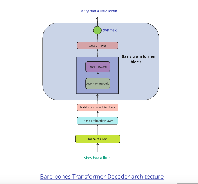
The attention-based transformer architecture in the paper ‘Attention is all you need‘ took its inspiration from the above Bahdanau paper and eventually evolved into the current Large Language Models (LLMs). The transformer architecture based on the attention mechanism was able to effectively address the shortcomings of the earlier RNNs. The architecture of the LLM is based on 2 key principles

a. An attention mechanism which determines the relationships between words in a sequence. It identifies how each word relates to others words in the sequence

b. A feed-forward neural network that takes the output of the attention module and enriches the relationships between the words

A final layer using softmax can predict the next word in a given sequence

LLM’s are based on the Transformer architecture. LLMs like ChatGPT, Claude, Cohere, Llama etc., typically go through 2 stages a) Pre-training b) Fine tuning

During pre-training the LLM is trained on a large corpus of unstructured text from the internet, wikipedia, arXiv, stack overflow etc. The pre-training helps the LLMs in general language understanding, enabling LLMs to learn grammar, syntax, context etc. This is followed by a fine-tuning phase where the language models is trained for specific domain or task using a smaller curated and annotated dataset of input, output pairs. This adjusts the weights of the LLM to handle the specific task in a particular domain. This may be further enhanced based on Reinforcement Learning with Human Feedback (RLHF) with reward-penalty for a given task during training. (In many ways, we humans also go through the stages of pre-training and fine-tuning in my opinion. As David Eagleman states above, we all come with a genetic blueprint based on millions of years of evolution of responses to triggers. During our early formative years this genetic DNA will create certain neural pathways in the brain akin to pre-training. Further from 2-5 years, through a couple of years of fine-tuning we learn a lot more – languages, recognition, emotion etc. This does simplify things to an extent but still I think to a large extent it holds)

Clearly, our brain is not only much more complex but also uses a minuscule energy about 60W to compute complex tasks, which is roughly equivalent to a light bulb. While for e.g. training GPT-3 which has 175 billion parameters, consumes an estimated 1287 MWH, which is roughly equivalent the consumption of an average US household for 120 years (Ref: https://adasci.org/how-much-energy-do-llms-consume-unveiling-the-power-behind-ai/?ts=1734961973)

NLP is based on the fact that human language is some ordered sequence of words. Moreover, words in a language are repetitive and thus inherently categorical. Hence, we need to use a technique for handling these categorical words for e.g. One-Hot-Encoding (OHE). But since the vocabulary of languages is extremely large, using OHE would become unmanageable. There are several other more efficient encoding methods available. Large Language Models (LLMs), which are the backbone of GenAI are trained on a large corpus of text spanning the internet, wikipedia, and other domains. The text is first converted into a numerical form through a process called tokenisation, where the words, subwords are assigned a numerical value based on some scheme. Tokenisation, can be at the character level, sub-word level, word level, sentence or even paragraph level. The choice of encoding is trade-off between vocabulary size vs sequence or context length. For character level encoding, the vocabulary will be around ~36 including letters, punctuation etc., but the sequences generated for sentences with this method will be very long. While word encodings will have a large vocabulary, an entire sentences can be captured in a shorter sequences. The encodings typically used are Byte Pair Encoding (BPE) from OpenAI, WordPiece or Sentence encoding. The sentences are first converted to tokens.

The tokens are then converted into embedding vectors which can 16, 32 or 128 real-valued dimensions. The embedding vectors convert the tokens into a multi-dimensional continuous space and capture the semantic meaning of the tokens as they get trained. The embeddings assigned, do not inherently capture the semantic meaning of words fully. But in a rough sort of way. For e.g. “I sat on the bank of a river” and “I deposited money in a bank”, the word bank may have the same embedding. But as the model is trained through the transformer with sequences of text passing through the attention module, the embeddings are updated with contextual information. So for e.g. in the 1st sentence “bank” will be associated with the word “river” and in the 2nd sentence the attention module will also capture the context of the “bank” and associate it with the word “money”

A transformer is well suited for predicting the next word in a given sequence. This is called a auto-regressive decoder-only model. The sequence of steps a enable a Transformer to be capable of predicting the next word in a given sequence is based on the following steps

a) Training on a large corpus of text from internet, wikipedia, books, and research repositories like arXiv etc

The text are tokenised based on one of the tokenisation schemes mentioned above like BPE, Wordpiece etc. to convert the words into numerical values

The tokens are then converted into multi-dimensional real-valued embedding vectors. The embeddings are vectors which through multiple iterations capture richer meaning context-aware meaning of sentences

The Attention module determines the affinity each word has to the other words in the sentence. This affinity can be captured over longer sentence structures too and this is based on the context (sequence) length depending on the size of the model.

The weights from the output of the Attention module then go to a simple 2 layer Feed Forward Neural Network (FFN) which tries to predict the next word in a sentence. For this each sentence is taken as input with the target being the same sentence shifted by one place.

For e,g,

Input: Mary had a little lamb

Target: had a little lamb <end>

So in a sentence w₁, w₂, w_3, … , w_n the FFN will use

w₁ to predict w₂

w₁ , w₂ to predict w₃ and so on
During back propagation, the error between the predicted word and the actual target word is calculated and propagated backwards through the network updating the weights and biases of the NN. The FFN uses tries to minimise the cross-entropy or log loss which computes the difference between the predicted probabilities and target values.

Attention module

For e.g. if we had the sentence “The quick brown fox jumped over the lazy dog”, Attention is computed as follows

Each word in the above sentence is tokenised and represented as dense vector. The transformer architecture uses 3 weight matrices call W_{q ,} W_k, W_v called the Query Weight, Key Weight and Value weight matrices which are learnable matrices. The embedding vectors of the sentence are multiplied with these W_q, W_k, W_v matrices to give Q (Query), K(Key) and V (Value) vectors.

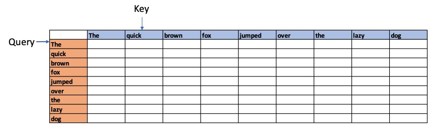
The dot product of the Query vector with all the Key vectors is performed. Since these are vectors, the dot product will determine the similarity or alignment, the query ‘The’ has for the each of the Keys. This is the fundamental concept of of the Attention module. This is because in a multi-dimensional vector space, vectors which are closer together will give a high dot product. Hence, the dot product between the Query and all the Keys gives the affinity the Query has to all other Keys. This is computed as the Attention Score.

For e,g the above process could show that quick and brown attend to the fox, and lazy attends to the dog – and they have relatively high Attention Scores compared to the rest. In addition the Attention operation may also determine that there is a relation between fox and dog in the sentence.

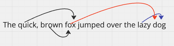
These affinities show up over several iterations through batches of sentences as W_q, W_K, W_v are learnable parameters. The relationship learned is depicted below

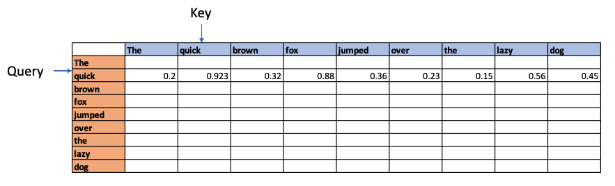
Next the values are normalised using the Softmax function since this will result in a mean of 0 and a variance of 1. This will give normalised attention scores

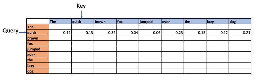
Causal attention. Since future words cannot affect the earlier words these values are made -Infinity so when we perform Softmax we get the value 0 for these values

Self-Attention Mechanism enables the model to evaluate the importance of tokens relative to each other. The self-attention mechanism is written as

$Attention(Q,K,V) = softmax(\frac{Q.K^{T}}{sqrt(d_{K})})V$

where Q, K, V are Query, Key and Value vectors and d_K is the dimensionality of the Key vectors. $\sqrt{d_{K}}$ scales the dot product so that the dot product values are not overly large

where the Scaled Attention score = $(\frac{Q.K^{T}}{sqrt(d_{K})})$

The Attention weights = softmax(Scaled Attention score)

$Attention Output = \sum Attention Weights * V_{j}$

This computes a context-aware representation of each token with respect to all other tokens

Feed Forward Network (FFN)

In the case of training a language model the fact that language is sequential enables the model to be trained on the language itself. This is done by training the model on large corpus of text, where the language learns to predict the next words in the sequence. So for example in the sentence

Feedforward Network (FFN) comprises two linear transformations separated by a non-linearity, typically modeled

with the first layer transformation as

$\sigma(xW_{1}+b_{1})$

and the second layer transformation is

$FFN(x)=\sigma(xW_{1}+b_{1})W_{2} + b_{2}$
where $W_{1}$ and $W_{2}$ are the weight matrices, and $b_{1}$ and $b_{2}$ are the biases

where $W_{1} = d_{model}$ x $d_{hidden}$ and

$W_{2} = d_{hidden}$ x $d_{model}$ and $d_{hidden}$ is usually 4 times the dimesnion of $d_{hidden}$

$\sigma$ is the activation function which can be ReLU, GELU or SwiGLU

Input to the FFN

The Decoder receives the output of the Self Attention module to the FFN network. This output from the Attention module is context-aware with the words in the input sequence having different affinities to other words in the sequence

The Target of the FFN is the input sequence shifted by one word

The output from the Attention head and the layer normalization

Normed Output = LayerNorm(Input+MultiHeadOutput)

In essence the Decoder only architecture can be boiled down to the following main modules

Tokenization – The input text is split either on characters, subwords, words, to convert the text into numbers
Vector Embedding – The numerical tokens are then converted into Dense vectors
Positional Embedding – The position order of the text sequence is encoded using the positional embedding. This positional embedding is added to the vector embedding
- Input embedding = Vector embedding + Positional embedding
Attention module – The attention module computes the affinity the different words have for other words in its vicinity. This is done through the the use of 3 weight matrices , , . By multiplyting these matrices with the input vectors we get Q,K and V vectors. The attention is computed as
- $Attention(Q,K,V)=softmax(\frac{Q.K^{T}}{\sqrt{d_{K}}})V$
For the decoder, attention is masked to prevent the model from looking at future tokens during training also known as causal attention mentioned above
The output pf the Attention module is passed to a 2 layer FFN which uses GeLU activation with Adam optimszation. This involves the following 2 steps
- Computing the cross-entropy (loss) using the predicted words and the actual labels
- Backpropagting the error through all the layers and updating the layer weights, $W_{Q}, W_{K}, W_{V}$
If the size of the FFN’s output is the vocabulary size then we can use
P(next word|context)=softmax(FFN output)
If the size of the model output is not the vocabulary size then the a final linear layer embeds the output to the size of the dictionary. This maps the model’s hidden states to the vocabulary size enabling the predicting of the next word from the vocabulary
Next word prediction : The next word prediction is done by applying softmax on the output of the FFN layer (logits) to compute the probability for the vocabulary
- P(next word∣context)=softmax(Logits)
After computing the probability the model selects the next word based on one of many options – to either choose the most probable word or on some other algorithm

The above sequence of steps is a bare-bones attention and transformer module. In of itself it can achieve little as the transformer module will have to contend with vanishing or exploding gradient issues. It needs additional bells and whistles to make it work effectively

Additional layers to the above architecture

a) Residual Connection and Layer Normalisation (Add + Norm) –

i) Residual, skip connections

Residual connection or skip connections are added the input of each layer to the output to enable the gradients to propagate effectively. This is based on the paper ‘Deep Residual Learning for Image Recognition” from Microsoft

Residual connections also known as skip or shortcut connections are performed by adding the input of layer to the output of the layer as a shortcut. This helps in preventing the vanishing gradient, because of the gradients become progressively smaller as they pass through successive layers.

ii) Layer normalisation

In addition layer normalisation is done to stabilise the activation across a single feature to have 0 mean and a variance of 1 by computing

Mean and variance calculation

$\mu = \frac{1}{D}\sum_{i=1}^{D}x_{i}$ , $\sigma ^{2} = \frac{1}{D} \sum_{i=1}^{D} (x_{i}-\mu)^{2}$

Normalization

$\hat{x_{i}} =\frac{x_{i-\mu}}{\sqrt{\sigma^{2}-\epsilon}}$

Layer normalization introduces learnable parameters using the equation

$y_{i} = \gamma \hat{x_{i}} +\beta$

This can be written as
ResidualOutput=Input+Output of Attention/FFN

The above statement mentions that the Input layer to the Attention /FFN module is added to the output to mitigate the vanishing gradient problem

NormedOutput=LayerNorm(Residual Output)

Layer Normalisation is then applied to the Residual Output to stabilise the activations.

b) Multi-headed Attention : Typically Transformer use multiple parallel heads of attention. Each head will compute a slightly different variations to the attention values, thus making the whole learning process richer. Multi-headed learning is capable of capturing more nuanced affinities of different words in the sentence to other words in the sentence/context.

c) Dropout : Dropout is a technique where random hidden units or neurons are dropped from the network during training. This prevents overfitting and helps to regularise/generalise the learning of the network. In Transformer Architectures, dropout is used after calculating the Attention Weights. Dropout can also be applied in the Feed Forward Network or in the Residual Connections

This is shown diagrammatically here

Points to note:

a) The Attention mechanism is able to pick out affinities between words in a sentence. This happens despite the fact the the W_Q, W_K, W_V matrices are randomly initialised. As the model trained iteratively through a large corpus of text using next token prediction for Auto Regressive Transformers and Masked prediction as in the case of BERT, then the affinities show up. This training allows the model to learn the contextual relationships and affinities words have with each other. The dot product Q, K measures the affinity words have for each other and will be high if they are highly related to each other. This is because they will aligned in a the multi-dimensional embedding space of these vectors, besides semantically and contextually related tokens are closer to each other.

b) The Feed Forward Network (FFN) in the Transformer’s Attention block is relatively small and has just 2 layers. This is for computational efficiency and deeper Neural Networks can increase costs. Moreover, it has been found that deeper and wider networks did not significantly improve performance while also preventing overfitting.

c) The above architecture is based on the Causal Attention, Decoder only transformer. The original paper includes both the encoder and the decoder to enable translation across different languages. In addition architectures like BERT use ‘masked attention’ and randomly mask words

The flow of vectors and dimensionality from the input sentence tokens to the output token prediction is as follows

a) For a batch (B) of 2 sentences with 6 words (T) each, where each word is converted into a token. If Byte Pair Encoding (BPE) is used then an integer value between 1-50257 will be obtained.

Input shape = (B x T) = (2 x 6)

b) Token embedding – Each token in the vocabulary is converted into an embedding vector of size $d_{model}$ = 512 dimension vector

Output shape = (B x T x $d_{model}$ ) = (2 x 6 x 512)

c) Positional embedding is added

Shape of positional embedding = T x $d_{model}$ = (6 x512)

d) Output shape with token and positional embedding is the same

Output shape = (B x T x $d_{model}$ ) = (2 x 6 x 512)

d) Multi-head attention

e) The W_Q, W_K, W_V learnable matrices are each of size

$d_{model}$ x $d_{model}$

f) Q = X x W_Q = (B x T x $d_{model}$ ) x ( $d_{model}$ x $d_{model}$ )

Output shape of Q, K, V = (B x T x $d_{model}$ ) = (2 x 6 x 512)

g) Number of heads h = 8

Dimensionality of each head = $d_{model}$ /8 = $d_{k}$ = 64

h) Splitting across the heads we have

Shape per head = (B, h, T, $d_{k}$ ) = ( 2, 8, 6, 64)

h) Weighted sum of values =

Output shape per head = (B, h, T, $d_{k}$ ) = ( 2, 8, 6, 64)

i) All the heads are concatenated

(B x T x $d_{model}$ ) = (2 x 6 x 512)

j) The FFN has one hidden layer which is 4 times $d_{model}$

$d_{hidden}$ = $d_{model}$ x 4

Final output of FFN after passing through hidden layer and back

Output shape =(B x T x $d_{model}$ ) = (2 x 6 x 512)

k) Residual, shortcut connections and layer norm do not change shape

Output shape =(B x T x $d_{model}$ ) = (2 x 6 x 512)

l) The final output is projected back into the original vocabulary space. For BPE it

50257.

Using a weight matrix (512 x vocab_size) = (512 x 50257)

Final output shape = (B x T x vocab_size) = (2 x 6 x 50257)

The output is in probabilities and hence gives the most likely next word in the sentence

Conclusion

This post tries to condense the key concepts around the Attention mechanism and the Transformer Architecture which have been the catalyst in the last few years, resulting in an explosion in the area of Gen AI, and there seems to be no stopping. It is indeed fascinating how the human language has been mathematically analysed for semantic meaning and relevance.

References

Building LLMs from Scratch by Sebastian Raschka
Hands-on Large Language Model by Jay Alammar, Maarten Grootendorst
Let’s build GPT from scratch: from scratch, in code, spelled out – Andrej Karpathy
Attention in Transformers, visually explained – 3Blue1Brown
Awesome LLM – Hannibal046 (collection of LLM papers)

Also see

To see all posts, click Index of posts

Video presentation on Machine Learning, Data Science, NLP and Big Data – Part 4

In this presentation I demonstrate some Shiny R apps that I have developed. The demo also includes googleMotion Charts using googleVis

Video presentation on Machine Learning, Data Science, NLP and Big Data – Part 3

This presentation includes the 3 part and touches upon Apache Edgent, NLP and Big Data with Spark.

Natural language processing: What would Shakespeare say?

Here is a scene from Christopher Nolan’s classic movie Interstellar. In this scene Cooper, a crew member of the Endurance spaceship which is on its way to 3 distant planets via a wormhole, is conversing with TARS which is one of US Marine Corps former robots some year in the future.

TARS (flippantly): “Everybody good? Plenty of slaves for my robot colony?”
TARS: [as Cooper repairs him] Settings. General settings. Security settings.
TARS: Honesty, new setting: ninety-five percent.
TARS: Confirmed. Additional settings.
Cooper: Humor, seventy-five percent.
TARS: Confirmed. Self-destruct sequence in T minus 10, 9…
Cooper: Let’s make that sixty percent.
TARS: Sixty percent, confirmed. Knock knock.
Cooper: You want fifty-five?

Natural Language has been an area of serious research for several decades ever since Alan Turing in 1950 proposed a test in which a human evaluator would simultaneously judge natural language conversations between another human and a machine, that is designed to generate human-like responses, behind a closed doors. If the responses of the human and machine were indistinguishable then we can say that the machine has passed the Turing test signifying machine intelligence.

How cool would it be if we could converse with a machines using Natural Language with all the subtleties of language including irony, sarcasm and humor? While considerable progress has been made in Natural Language Processing for e.g. Watson, Siri and Cortana the ability to handle nuances like humor, sarcasm is probably many years away.

This post looks at one aspect of Natural Language Processing, particularly in dealing with the ability to predict the next word(s) given a word or phrase.

This title of this post should really be ‘Natural language Processing: What would Shakespeare say, and what would you say’ because this post includes two interactive apps that can predict the next word

a) The first app given a (Shakespearean) phrase will predict the most likely word that Shakespeare would have said
Try the Shiny app : What would Shakespeare have said?

b) The second app will, given a regular phrase predict the next word(s) in regular day to day English usage
Try the Shiny app: What would you say?

Checkout my book ‘Deep Learning from first principles- In vectorized Python, R and Octave’. My book is available on Amazon as paperback ($16.99) and in kindle version($6.65/Rs449).

You may also like my companion book “Practical Machine Learning with R and Python:Second Edition- Machine Learning in stereo” available in Amazon in paperback($10.99) and Kindle($7.99/Rs449) versions.

Natural Language Processing (NLP) is a field of computer science, artificial intelligence, and computational linguistics concerned with the interactions between computers and human (natural) languages. NLP encompasses many areas from computer science besides inputs from the domain of linguistics , psychology, information theory, mathematics and statistics

However NLP is a difficult domain as each language has its own quirkiness and ambiguities, and English is no different. Let us take the following 2 sentences

Time flies like an arrow.
Fruit flies like a banana.

Clearly the 2 sentences mean entirely different things when referencing the words ‘flies like’. The English language is filled with many such ambiguous constructions

There have been 2 main approaches to Natural Language Processing – The rationalist approach and the empiricist’s approach. The empiricists approached natural language as a data driven problem based on statistics while the rationalist school led by Noam Chomsky, the linguist, strongly believed that sentence structure should be analyzed at a deeper level than mere surface statistics.

In his book Syntactic Structures, Chomsky introduces a famous example of his criticism of finite-state probabilistic models. He cites 2 sentences (a) ‘colorless green ideas sleep furiously’ (b) ‘furiously sleep ideas green colorless’. Chomsky’s contention is that while neither sentence or any of its parts, have ever occurred in the past linguistic experience of English it can be easily inferred that (a) is grammatical, while (b) is not. Chomsky argument is that sentence structure is critical to Natural Language processing of any kind. Here is a good post by Peter Norvig ‘On Chomsky and the two cultures of statistical learning’. In fact, from 1950 to the 1980s the empiricists approach fell out of favor while reasonable progress was made based on rationalist approach to NLP.

The return of the empiricists
But thanks to great strides in processing power and the significant drop in hardware the empiricists approach to Natural Language Processing made a comeback in the mid 1980s. The use of probabilistic language models combined with the increase in the power of processing saw the rise of the empiricists again. Also there had been significant improvement in machine learning algorithms which allowed the use of the computing resources more efficiently.

In this post I showcase 2 Shiny apps written in R that predict the next word given a phrase using statistical approaches, belonging to the empiricist school of thought. The 1^st one will try to predict what Shakespeare would have said given a phrase (Shakespearean or otherwise) and the 2^nd is a regular app that will predict what we would say in our regular day to day conversation. These apps will predict the next word as you keep typing in each word.

In NLP the first step is a to build a language model. In order to build a language model the program ingests a large corpora of documents. For the a) Shakespearean app, the corpus is the “Complete Works of Shakespeare“. This is also available in Free ebooks by Project Gutenberg but you will have to do some cleaning and tokenzing before using it. For the b) regular English next word predicting app the corpus is composed of several hundred MBs of tweets, news items and blogs.

Once the corpus is ingested the software then creates a n-gram model. A 1-gram model is representation of all unique single words and their counts. Similarly a bigram model is representation of all 2 words and their counts found in the corpus. Similar we can have trigram, quadgram and n-gram as required. Typically language models don’t go beyond 5-gram as the processing power needed increases for these larger n-gram models.

The probability of a sentence can be determined using the chain rule. This is shown for the bigram model below where P(s) is the probability of a sentence ‘s’
P( The quick brown fox jumped) =
P(The) P(quick|The) P(brown|The quick) * P(fox||The quick brown) *P(jumped|The quick brown fox)
where BOS -> is the beginning of the sentence and

P(quick|The) – The probability of the word being ‘quick’ given that the previous word was ‘The’. This probability can be approximated based on Markov’s chain rule which allows that the we can compute the conditional probability
$P(w|w_{i})$

of a word based on a couple of its preceding words. Hence this allows this approximation as follows
$P(w{_{i}}|w_{1}w_{2}w_{3}..w_{i-1}) = P(w{_{i}}|w_{i-1})$

The Maximum Likelihood Estimate (MLE) is given as follows for a bigram
$P_{MLE}(w_{i}|w_{i-1}) = count(w_{i-1},w_{i})/count(w_{i-1})$
$P_{MLE}(w_{i}|w_{i-1}) = c(w_{i-1},w_{i})/c(w_{i-1})$

Hence for a corpus
We can calculate the maximum likelihood estimates of a given word from its previous word. This computation of the MLE can be extended to the trigram and the quadgram

For a trigram
$P(w_{i}|w_{i-1}w_{i-2}) = c(w_{i-2}w_{i-1},w_{i})/c(w_{i-2}w_{i-1})$

Smoothing techniques
The MLE estimates for many bigrams and trigrams will be 0, because we may have not have yet seen certain combinations. But the fact that we have not seen these combinations in the corpus should not mean that they could never occur, So the MLE for the bigrams, trigrams etc have be smoothed so that it does not have a 0 conditional probability. One such method is to use ‘Laplace smoothing’. This smoothing tries to steal from the probability mass of words that occur in the corpus and re-distribute it to the words that do not occur in the corpus. In a way this equivalent to probability mass stealing. This is the simplest smoothing technique and is also known as the ‘add +1’ smoothing technique and requires that 1 be added to all counts

So the MLE below
$P_{MLE}(w_{i}|w_{i-1}) = c(w_{i-1},c_{i})/c(w_{i-1})$

With the add +1 smoothing this becomes
$P_{MLE}(w_{i}|w_{i-1}) = c(w_{i-1},c_{i})+1/c(w_{i-1})+V$

This smoothing is done for bigram, trigam and quadgram. Smoothing is usually used with an associated technique called ‘backoff’. If the phrase is not found in a n-gram model then we need to backoff to a n-1 gram model. For e.g. a lookup will be done in quadgrams, if not found the algorithm will backoff to trigram, bigram and finally to unigram.

Hence if we had the phrase
“on my way”

The smoothed MLE for a quadgram will be checked for the next word. If this is not found this is backed of my searching smoothed MLEs for trigrams for the phrase ‘my way’ and if this not found search the bigram for the next word to ‘way’.

One such method is the Katz backoff which is given by which is based on the following method
Bigrams with nonzero count are discounted according to discount ratio d_{r} (i.e. the unigram model).
$r^{*}=(r+1)n_{r+1}/n_{_{r}}$
$d_{r} = r^{*}/r$

Count mass subtracted from nonzero counts is redistributed among the zero-count bigrams according to next lower-order distribution

A better performance is obtained with the Kneser-Ney algorithm which computes the continuation probability of words. The Kneser-Ney algorithm is included below
$P_{\mathit{KN}}(w_i \mid w_{i-1}) = \dfrac{\max(c(w_{i-1} w_i) - \delta, 0)}{\sum_{w'} c(w_{i-1} w')} + \lambda \dfrac{\left| \{ w_{i-1} : c(w_{i-1}, w_i) > 0 \} \right|}{\left| \{ w_{j-1} : c(w_{j-1},w_j) > 0\} \right|}$

where
$\lambda(w_{i-1}) = \dfrac{\delta}{c(w_{i-1})} \left| \{w' : c(w_{i-1}, w') > 0\} \right|$

This post was inspired by the final Capstone Project in which I had to create a Shiny app for predicting the next word as a part of Data Science Specialization conducted by John Hopkins University, Bloomberg School of Public health at Coursera.

I further extended this concept where I try to predict what Shakespeare would have said. For this I ingest the Complete Works of Shakespeare which is the corpus. The +1 Add smoothing with Katz backoff and the Kneser-Ney algorithm on the unigram, bigram, trigram and quadgrams were then implemented.

Note: This post in no way tries to belittle the genius of Shakespeare. From the table below it can be seen that our day to day conversation has approximately 210K, 181K & 65K unique bigrams, trigrams and quadgrams. On the other hand, Shakespearean literature has 271K, 505K, & 517K bigrams, trigrams and quadgrams. It can be seen that Shakespeare had a rich and complex set of word combination.

Not surprisingly the computation of the conditional and continuation probabilities for the Shakespearean literature is orders of magnitude larger.
Here is a small table as comparison

This implementation was done entirely using R. The main R packages used for this implementation were tm,Rweka,dplyr. Here is a slide deck on the the implementation details of the apps and key lessons learnt: PredictNextWord
Unfortunately I will not be able to include the implementation details as I am bound by The Coursera Honor Code.

If you have not already given the apps a try do give them a try
Try the Shiny apps
– What would Shakespeare say?
– What would you say?

References
a. http://www.foldl.me/2014/kneser-ney-smoothing/
b. http://mkoerner.de/media/bachelor-thesis.pdf
c. https://www.coursera.org/course/nlp (Week 2)
d. http://www.cs.berkeley.edu/~klein/cs294-5/chen_goodman.pdf

Also see
1. Re-working the Lucy-Richardson Algorithm in OpenCV
2. What’s up Watson? Using IBM Watson’s QAAPI with Bluemix, NodeExpress – Part 1
3. Bend it like Bluemix, MongoDB with autoscaling – Part 2
4. TWS-4: Gossip protocol: Epidemics and rumors to the rescue
5. Thinking Web Scale (TWS-3): Map-Reduce – Bring compute to data
6. Deblurring with OpenCV:Weiner filter reloaded

What’s up Watson? Using IBM Watson’s QAAPI with Bluemix, NodeExpress – Part 1

Published in IBM developerWorks ‘Whats up Watson? Using Watson QAAPI with Bluemix and NodeExpress‘

In this post I take the famed IBM Watson through the paces (yes, that’s right!, this post is about using the same IBM Watson which trounced 2 human Jeopardy titans in a classic duel in 2011). IBM’s Watson (see What is Watson?) is capable of understanding the nuances of the English language and heralds a new era in the domain of cognitive computing. IBM Bluemix now includes 8 services from Watson ranging from Concept Expansion, Language Identification, Machine Translation, Question-Answer etc. For more information on Watson’s QAAPI and the many services that have been included in Bluemix please see Watson Services.

In this article I create an application on IBM Bluemix and use Watson’s QAAPI (Question-Answer API) as a service to the Bluemix application. For the application I have used NodeExpress to create a Webserver and post the REST queries to Watson. Jade is used format the results of Watson’s Response.

In this current release of Bluemix Watson comes with a corpus of medical facts. In other words Watson has been made to ingest medical documents in multiple formats (doc, pdf, html, text etc) and the user can pose medical questions to Dr.Watson. In its current avatar, its medical diet consisted of dishes from (CDC Health Topics, National Heart, Lung, and Blood Institute (NHLBI) National Institute of Arthritis and Musculoskeletal and Skin Diseases (NIAMS), National Institute of Diabetes and Digestive and Kidney Diseases (NIDDK), National Institute of Neurological Disorders and Stroke (NINDS), Cancer.gov (physician data query) etc.)

Try out my Watson app on Bluemix here – Whats up Watson?

To get down to Watson QAAPI business with Bluemix app you can fork the code from Devops at whatsup. This can then be downloaded to your local machine. You can also clone the code from GitHub at whatsup

To get started go to the directory where you have cloned the code for Whatsup app

2.Push the app to Bluemix using Cloud Foundry’s ‘cf’ commands as shown below

cf login -a https://api.ng.bluemix.net
3. Next push the app to Bluemix
cf push whatsup –p . –m 512M

In the Bluemix dashboard you should see ‘whatsup’ app running. Now click ‘Add Service’ and under Watson add ‘Question Answer’

Add Qatson QAAPI

You will be prompted with ‘Restage Application’. Click ‘Ok’. Once you have the app running you should be able to get started with Doc Watson.

The code for this Bluemix app with QAAPI as a Service is based on the following article Examples using the Question and Answer API

Here’s a look at the code for the Bluemix & Watson app.

In this Bluemix app I show the different types of Questions we can ask Watson and the responses we get from it. The app has a route for each of the different types of questions and options

a. Simple Synchronous Query: Post a simple synchronous query to Watson
This is the simplest query that we can pose to Watson. Here we need to just include the text of the question and the also a Sync Timeout. The Sync Timeout denotes the time client will wait for responses from the Watson service
// Ask Watson a simple synchronous query
app.get('/question',question.list); app.post('/simplesync',simplesync.list);
b. Evidence based question: Ask Watson to respond to evidence given to it
Ask Watson for responses based on evidence given like medical conditions etc. This would be a used for diagnostic purposes I would presume.
// Ask Watson for responses based on evidence provided
app.get('/evidence',evidence.list); app.post('/evidencereq',evidencereq.list);
c. Request for a specified set of answers to a question: Ask Dr. Watson to give a specified number of responses to a question
// Ask Watson to provide specified number of responses to a query
app.get('/items',items.list); app.post('/itemsreq',itemsreq.list);
d. Get a formatted response to a question: Ask Dr. Watson to format the response to the question
// Get a formatted response from Watson for a query
app.get('/format',format.list); app.post('/formatreq',formatreq.list);

To get started with Watson we would need to connect the Bluemix app to the Watson’s QAAPI as a service by parsing the environment variable. This is shown below

//Get the VCAP environment variables to connect Watson service to the Bluemix application

question.js
o o o if (process.env.VCAP_SERVICES) { var VCAP_SERVICES = JSON.parse(process.env.VCAP_SERVICES); // retrieve the credential information from VCAP_SERVICES for Watson QAAPI var hostname = VCAP_SERVICES["Watson QAAPI-0.1"][0].name; var passwd = VCAP_SERVICES["Watson QAAPI-0.1"][0].credentials.password; var userid = VCAP_SERVICES["Watson QAAPI-0.1"][0].credentials.userid; var watson_url = VCAP_SERVICES["Watson QAAPI-0.1"][0].credentials.url;

Next we need to format the header for the POST request

var parts = url.parse(watson_url); // Create the request options to POST our question to Watson var options = {host: parts.hostname, port: 443, path: parts.pathname, method: 'POST', headers: headers, rejectUnauthorized: false, // ignore certificates requestCert: true, agent: false};

The question that is to be asked of Watson needs to be formatted appropriately based on the input received in the appropriate form (for e.g. simplesync.jade)

question.js
// Get the values from the form var syncTimeout = req.body.timeout; var query = req.body.query; // create the Question text to ask Watson var question = {question : {questionText :query }}; var evidence = {"evidenceRequest":{"items":1,"profile":"yes"}}; // Set the POST body and send to Watson req.write(JSON.stringify(question)); req.write("\n\n"); req.end();

Now you POST the Question to Dr. Watson and receive the stream of response using Node.js’ .on(‘data’,) & .on(‘end’) shown below

question.js
…..
var req = https.request(options, function(result) {
// Retrieve and return the result back to the client
result.on(“data”, function(chunk) {
output += chunk;
});

result.on('end', function(chunk) { // Capture Watson's response in output. Parse Watson's answer for the fields var results = JSON.parse(output); res.render( 'answer', { "results":results }); }); });

The results are parsed and formatted displayed using Jade. For the Jade templates I have used a combination of Jade and inline HTML tags (Jade can occasionally be very stubborn and make you sweat quite a bit. So I took the easier route of inline HTML tagging. In a later post I will try out CSS stylesheets to format the response.)

Included below is the part of the jade template with inline HTML tagging

Answer.jade
o o o <h2 style="color:blueviolet"> Question Details </style> </h2> for result in results.question.qclasslist p <font color="blueviolet"> Value = <font color="black "> #{result.value} </font> p <font color="blueviolet"> Focuslist </font> = <font color="black "> #{results.question.focuslist[0].value} </font> // The 'How' query's response does not include latlist. Hence conditional added. if latlist p <font color="blueviolet"> Latlist </font> = <font color="black "> #{results.question.latlist[0].value} </font>

o o o

Now that the code is all set you can fire the Watson. To do this click on the route

Click the route whatsup.mybluemix.net and ‘Lo and behold’ you should see Watson ready and raring to go.

As the display shows there are 4 different Question-Answer options that there is for Watson QAAPI

Simple Synchronous Question-Answer
This option is the simplest option. Here we need to just include the text of the question and the also a Sync Timeout. The question can be any medical related question as Watson in its current Bluemix avatar has a medical corpus

For e.g.1) What is carotid artery disease?

2) What is the difference between hepatitis A and hepatitis B etc.

The Sync Timeout parameter specifies the number of seconds the QAAPI client will wait for the streaming response from Watson. An example question and Watson’s response are included below

;

When we click Submit Watson spews out the following response

Evidence based response:

In this mode of operation, questions can be posed to Watson based on observed evidence. Watson will output all relevant information based on the evidence provided. As seen in the output Watson provides a “confidence factor” for each of its response

Watson gives response with appropriate confidence values based on the given evidence

Question with specified number of responses
In this option we can ask Watson to provide us with at least ‘n’ items in its response. If it cannot provide as many items it will give an error notification

This will bring up the following screen where the question asked is “What is the treatment for Down’s syndrome?” and Items as 3.

Watson gives 3 items in the response as shown below

Formatted Response: Here Watson gives a formatted response to question asked. Since I had already formatted the response using Jade it does not do extra formatting as seen in the screen shot.

Updated synonym based response. In this response we can change the synonym list based on which Watson will search its medical corpus and modify its response. The synonym list for the the question “What is fever?” is shown below. We can turn off synonyms by setting to ‘false’ and possibly adding other synonyms for the search

This part of the code has not been included in this post and is left as an exercise to the reader 🙂

As mentioned before you can fork and clone the code from IBM devops at whatsup or clone from GitHub at whatsup

There are many sections to Watson’s answer which cannot be included in this post as the amount of information is large and really needs to be pared to pick out important details. I am including small sections from each part of Watson’s response below to the question “How is carotid artery disease treated/”

I will follow up this post with another post where I will take a closer look at Watson’s response which has many parts to it
namely

– Question Details