R vs Python: Different similarities and similar differences

A debate about which language is better suited for Datascience, R or Python, can set off diehard fans of these languages into a tizzy. This post tries to look at some of the different similarities and similar differences between these languages. To a large extent the ease or difficulty in learning R or Python is subjective. I have heard that R has a steeper learning curve than Python and also vice versa. This probably depends on the degree of familiarity with the languuge To a large extent both R an Python do the same thing in just slightly different ways and syntaxes. The ease or the difficulty in the R/Python construct’s largely is in the ‘eyes of the beholder’ nay, programmer’ we could say. I include my own experience with the languages below.

Check out my compact and minimal book “Practical Machine Learning with R and Python:Third edition- Machine Learning in stereo” available in Amazon in paperback($12.99) and kindle($8.99) versions. My book includes implementations of key ML algorithms and associated measures and metrics. The book is ideal for anybody who is familiar with the concepts and would like a quick reference to the different ML algorithms that can be applied to problems and how to select the best model. Pick your copy today!!

1. R data types

R has the following data types

Character
Integer
Numeric
Logical
Complex
Raw

Python has several data types

Int
float
Long
Complex and so on

2. R Vector vs Python List

A common data type in R is the vector. Python has a similar data type, the list

# R vectors
a<-c(4,5,1,3,4,5)
print(a[3])

## [1] 1

print(a[3:4]) # R does not always need the explicit print.

## [1] 1 3

#R type of variable
print(class(a))

## [1] "numeric"

# Length of a
print(length(a))

## [1] 6

# Python lists
a=[4,5,1,3,4,5] # 
print(a[2]) # Some python IDEs require the explicit print
print(a[2:5])
print(type(a))
# Length of a
print(len(a))

## 1
## [1, 3, 4]
## 
## 6

2a. Other data types – Python

Python also has certain other data types like the tuple, dictionary etc as shown below. R does not have as many of the data types, nevertheless we can do everything that Python does in R

# Python tuple
b = (4,5,7,8)
print(b)


#Python dictionary
c={'name':'Ganesh','age':54,'Work':'Professional'}
print(c)
#Print type of variable c

## (4, 5, 7, 8)
## {'name': 'Ganesh', 'age': 54, 'Work': 'Professional'}

2.Type of Variable

To know the type of the variable in R we use ‘class’, In Python the corresponding command is ‘type’

#R - Type of variable
a<-c(4,5,1,3,4,5)
print(class(a))

## [1] "numeric"

#Python - Print type of tuple a
a=[4,5,1,3,4,5]
print(type(a))
b=(4,3,"the",2)
print(type(b))

## 
##

3. Length

To know length in R, use length()

#R - Length of vector
# Length of a
a<-c(4,5,1,3,4,5)
print(length(a))

## [1] 6

To know the length of a list,tuple or dict we can use len()

# Python - Length of list , tuple etc
# Length of a
a=[4,5,1,3,4,5]
print(len(a))
# Length of b
b = (4,5,7,8)
print(len(b))

## 6
## 4

4. Accessing help

To access help in R we use the ‘?’ or the ‘help’ function

#R - Help - To be done in R console or RStudio
#?sapply
#help(sapply)

Help in python on any topic involves

#Python help - This can be done on a (I)Python console
#help(len)
#?len

5. Subsetting

The key difference between R and Python with regards to subsetting is that in R the index starts at 1. In Python it starts at 0, much like C,C++ or Java To subset a vector in R we use

#R - Subset
a<-c(4,5,1,3,4,8,12,18,1)
print(a[3])

## [1] 1

# To print a range or a slice. Print from the 3rd to the 5th element
print(a[3:6])

## [1] 1 3 4 8

Python also uses indices. The difference in Python is that the index starts from 0/

#Python - Subset
a=[4,5,1,3,4,8,12,18,1]
# Print the 4th element (starts from 0)
print(a[3])

# Print a slice from 4 to 6th element
print(a[3:6])

## 3
## [3, 4, 8]

6. Operations on vectors in R and operation on lists in Python

In R we can do many operations on vectors for e.g. element by element addition, subtraction, exponentation,product etc. as show

#R - Operations on vectors
a<- c(5,2,3,1,7)
b<- c(1,5,4,6,8)

#Element wise Addition
print(a+b)

## [1]  6  7  7  7 15

#Element wise subtraction
print(a-b)

## [1]  4 -3 -1 -5 -1

#Element wise product
print(a*b)

## [1]  5 10 12  6 56

# Exponentiating the elements of a vector
print(a^2)

## [1] 25  4  9  1 49

In Python to do this on lists we need to use the ‘map’ and the ‘lambda’ function as follows

# Python - Operations on list
a =[5,2,3,1,7]
b =[1,5,4,6,8]

#Element wise addition with map & lambda
print(list(map(lambda x,y: x+y,a,b)))
#Element wise subtraction
print(list(map(lambda x,y: x-y,a,b)))
#Element wise product
print(list(map(lambda x,y: x*y,a,b)))
# Exponentiating the elements of a list
print(list(map(lambda x: x**2,a)))

## [6, 7, 7, 7, 15]
## [4, -3, -1, -5, -1]
## [5, 10, 12, 6, 56]
## [25, 4, 9, 1, 49]

However if we create ndarrays from lists then we can do the element wise addition,subtraction,product, etc. like R. Numpy is really a powerful module with many, many functions for matrix manipulations

import numpy as np
a =[5,2,3,1,7]
b =[1,5,4,6,8]
a=np.array(a)
b=np.array(b)
#Element wise addition
print(a+b)
#Element wise subtraction
print(a-b)
#Element wise product
print(a*b)
# Exponentiating the elements of a list
print(a**2)

## [ 6  7  7  7 15]
## [ 4 -3 -1 -5 -1]
## [ 5 10 12  6 56]
## [25  4  9  1 49]

7. Getting the index of element

To determine the index of an element which satisifies a specific logical condition in R use ‘which’. In the code below the index of element which is equal to 1 is 4

# R - Which
a<- c(5,2,3,1,7)
print(which(a == 1))

## [1] 4

In Python array we can use np.where to get the same effect. The index will be 3 as the index starts from 0

# Python - np.where
import numpy as np
a =[5,2,3,1,7]
a=np.array(a)
print(np.where(a==1))

## (array([3], dtype=int64),)

8. Data frames

R, by default comes with a set of in-built datasets. There are some datasets which come with the SkiKit- Learn package

# R 
# To check built datasets use
#data() - In R console or in R Studio
#iris - Don't print to console

We can use the in-built data sets that come with Scikit package

#Python
import sklearn as sklearn
import pandas as pd
from sklearn import datasets
# This creates a Sklearn bunch
data = datasets.load_iris()
# Convert to Pandas dataframe
iris = pd.DataFrame(data.data, columns=data.feature_names)

9. Working with dataframes

With R you can work with dataframes directly. For more complex dataframe operations in R there are convenient packages like dplyr, reshape2 etc. For Python we need to use the Pandas package. Pandas is quite comprehensive in the list of things we can do with data frames The most common operations on a dataframe are

Check the size of the dataframe
Take a look at the top 5 or bottom 5 rows of dataframe
Check the content of the dataframe

a.Size

In R use dim()

#R - Size
dim(iris)

## [1] 150   5

For Python use .shape

#Python - size
import sklearn as sklearn
import pandas as pd
from sklearn import datasets
data = datasets.load_iris()
# Convert to Pandas dataframe
iris = pd.DataFrame(data.data, columns=data.feature_names)
iris.shape

b. Top & bottom 5 rows of dataframe

To know the top and bottom rows of a data frame we use head() & tail as shown below for R and Python

#R 
head(iris,5)

##   Sepal.Length Sepal.Width Petal.Length Petal.Width Species
## 1          5.1         3.5          1.4         0.2  setosa
## 2          4.9         3.0          1.4         0.2  setosa
## 3          4.7         3.2          1.3         0.2  setosa
## 4          4.6         3.1          1.5         0.2  setosa
## 5          5.0         3.6          1.4         0.2  setosa

tail(iris,5)

##     Sepal.Length Sepal.Width Petal.Length Petal.Width   Species
## 146          6.7         3.0          5.2         2.3 virginica
## 147          6.3         2.5          5.0         1.9 virginica
## 148          6.5         3.0          5.2         2.0 virginica
## 149          6.2         3.4          5.4         2.3 virginica
## 150          5.9         3.0          5.1         1.8 virginica

#Python
import sklearn as sklearn
import pandas as pd
from sklearn import datasets
data = datasets.load_iris()
# Convert to Pandas dataframe
iris = pd.DataFrame(data.data, columns=data.feature_names)
print(iris.head(5))
print(iris.tail(5))

##    sepal length (cm)  sepal width (cm)  petal length (cm)  petal width (cm)
## 0                5.1               3.5                1.4               0.2
## 1                4.9               3.0                1.4               0.2
## 2                4.7               3.2                1.3               0.2
## 3                4.6               3.1                1.5               0.2
## 4                5.0               3.6                1.4               0.2
##      sepal length (cm)  sepal width (cm)  petal length (cm)  petal width (cm)
## 145                6.7               3.0                5.2               2.3
## 146                6.3               2.5                5.0               1.9
## 147                6.5               3.0                5.2               2.0
## 148                6.2               3.4                5.4               2.3
## 149                5.9               3.0                5.1               1.8

c. Check the content of the dataframe

#R
summary(iris)

##   Sepal.Length    Sepal.Width     Petal.Length    Petal.Width   
##  Min.   :4.300   Min.   :2.000   Min.   :1.000   Min.   :0.100  
##  1st Qu.:5.100   1st Qu.:2.800   1st Qu.:1.600   1st Qu.:0.300  
##  Median :5.800   Median :3.000   Median :4.350   Median :1.300  
##  Mean   :5.843   Mean   :3.057   Mean   :3.758   Mean   :1.199  
##  3rd Qu.:6.400   3rd Qu.:3.300   3rd Qu.:5.100   3rd Qu.:1.800  
##  Max.   :7.900   Max.   :4.400   Max.   :6.900   Max.   :2.500  
##        Species  
##  setosa    :50  
##  versicolor:50  
##  virginica :50  
##                 
##                 
##

str(iris)

## 'data.frame':    150 obs. of  5 variables:
##  $ Sepal.Length: num  5.1 4.9 4.7 4.6 5 5.4 4.6 5 4.4 4.9 ...
##  $ Sepal.Width : num  3.5 3 3.2 3.1 3.6 3.9 3.4 3.4 2.9 3.1 ...
##  $ Petal.Length: num  1.4 1.4 1.3 1.5 1.4 1.7 1.4 1.5 1.4 1.5 ...
##  $ Petal.Width : num  0.2 0.2 0.2 0.2 0.2 0.4 0.3 0.2 0.2 0.1 ...
##  $ Species     : Factor w/ 3 levels "setosa","versicolor",..: 1 1 1 1 1 1 1 1 1 1 ...

#Python
import sklearn as sklearn
import pandas as pd
from sklearn import datasets
data = datasets.load_iris()
# Convert to Pandas dataframe
iris = pd.DataFrame(data.data, columns=data.feature_names)
print(iris.info())

## 
## RangeIndex: 150 entries, 0 to 149
## Data columns (total 4 columns):
## sepal length (cm)    150 non-null float64
## sepal width (cm)     150 non-null float64
## petal length (cm)    150 non-null float64
## petal width (cm)     150 non-null float64
## dtypes: float64(4)
## memory usage: 4.8 KB
## None

d. Check column names

#R
names(iris)

## [1] "Sepal.Length" "Sepal.Width"  "Petal.Length" "Petal.Width" 
## [5] "Species"

colnames(iris)

## [1] "Sepal.Length" "Sepal.Width"  "Petal.Length" "Petal.Width" 
## [5] "Species"

#Python
import sklearn as sklearn
import pandas as pd
from sklearn import datasets
data = datasets.load_iris()
# Convert to Pandas dataframe
iris = pd.DataFrame(data.data, columns=data.feature_names)
#Get column names
print(iris.columns)

## Index(['sepal length (cm)', 'sepal width (cm)', 'petal length (cm)',
##        'petal width (cm)'],
##       dtype='object')

e. Rename columns

In R we can assign a vector to column names

#R
colnames(iris) <- c("lengthOfSepal","widthOfSepal","lengthOfPetal","widthOfPetal","Species")
colnames(iris)

## [1] "lengthOfSepal" "widthOfSepal"  "lengthOfPetal" "widthOfPetal" 
## [5] "Species"

In Python we can assign a list to s.columns

#Python
import sklearn as sklearn
import pandas as pd
from sklearn import datasets
data = datasets.load_iris()
# Convert to Pandas dataframe
iris = pd.DataFrame(data.data, columns=data.feature_names)
iris.columns = ["lengthOfSepal","widthOfSepal","lengthOfPetal","widthOfPetal"]
print(iris.columns)

## Index(['lengthOfSepal', 'widthOfSepal', 'lengthOfPetal', 'widthOfPetal'], dtype='object')

f.Details of dataframe

#Python
import sklearn as sklearn
import pandas as pd
from sklearn import datasets
data = datasets.load_iris()
# Convert to Pandas dataframe
iris = pd.DataFrame(data.data, columns=data.feature_names)
print(iris.info())

## 
## RangeIndex: 150 entries, 0 to 149
## Data columns (total 4 columns):
## sepal length (cm)    150 non-null float64
## sepal width (cm)     150 non-null float64
## petal length (cm)    150 non-null float64
## petal width (cm)     150 non-null float64
## dtypes: float64(4)
## memory usage: 4.8 KB
## None

g. Subsetting dataframes

# R
#To subset a dataframe 'df' in R we use df[row,column] or df[row vector,column vector]
#df[row,column]
iris[3,4]

## [1] 0.2

#df[row vector, column vector]
iris[2:5,1:3]

##   lengthOfSepal widthOfSepal lengthOfPetal
## 2           4.9          3.0           1.4
## 3           4.7          3.2           1.3
## 4           4.6          3.1           1.5
## 5           5.0          3.6           1.4

#If we omit the row vector, then it implies all rows or if we omit the column vector
# then implies all columns for that row
iris[2:5,]

##   lengthOfSepal widthOfSepal lengthOfPetal widthOfPetal Species
## 2           4.9          3.0           1.4          0.2  setosa
## 3           4.7          3.2           1.3          0.2  setosa
## 4           4.6          3.1           1.5          0.2  setosa
## 5           5.0          3.6           1.4          0.2  setosa

# In R we can all specific columns by column names
iris$Sepal.Length[2:5]

## NULL

#Python
# To select an entire row we use .iloc. The index can be used with the ':'. If 
# .iloc[start row: end row]. If start row is omitted then it implies the beginning of
# data frame, if end row is omitted then it implies all rows till end
#Python
import sklearn as sklearn
import pandas as pd
from sklearn import datasets
data = datasets.load_iris()
# Convert to Pandas dataframe
iris = pd.DataFrame(data.data, columns=data.feature_names)
print(iris.iloc[3])
print(iris[:5])
# In python we can select columns by column name as follows
print(iris['sepal length (cm)'][2:6])
#If you want to select more than 2 columns then you must use the double '[[]]' since the 
# index is a list itself
print(iris[['sepal length (cm)','sepal width (cm)']][4:7])

## sepal length (cm)    4.6
## sepal width (cm)     3.1
## petal length (cm)    1.5
## petal width (cm)     0.2
## Name: 3, dtype: float64
##    sepal length (cm)  sepal width (cm)  petal length (cm)  petal width (cm)
## 0                5.1               3.5                1.4               0.2
## 1                4.9               3.0                1.4               0.2
## 2                4.7               3.2                1.3               0.2
## 3                4.6               3.1                1.5               0.2
## 4                5.0               3.6                1.4               0.2
## 2    4.7
## 3    4.6
## 4    5.0
## 5    5.4
## Name: sepal length (cm), dtype: float64
##    sepal length (cm)  sepal width (cm)
## 4                5.0               3.6
## 5                5.4               3.9
## 6                4.6               3.4

h. Computing Mean, Standard deviation

#R 
#Mean
mean(iris$lengthOfSepal)

## [1] 5.843333

#Standard deviation
sd(iris$widthOfSepal)

## [1] 0.4358663

#Python
#Mean
import sklearn as sklearn
import pandas as pd
from sklearn import datasets
data = datasets.load_iris()
# Convert to Pandas dataframe
iris = pd.DataFrame(data.data, columns=data.feature_names)
# Convert to Pandas dataframe
print(iris['sepal length (cm)'].mean())
#Standard deviation
print(iris['sepal width (cm)'].std())

## 5.843333333333335
## 0.4335943113621737

i. Boxplot

Boxplot can be produced in R using baseplot

#R
boxplot(iris$lengthOfSepal)

Matplotlib is a popular package in Python for plots

#Python
import sklearn as sklearn
import pandas as pd
import matplotlib.pyplot as plt
from sklearn import datasets
data = datasets.load_iris()
# Convert to Pandas dataframe
iris = pd.DataFrame(data.data, columns=data.feature_names)
img=plt.boxplot(iris['sepal length (cm)'])
plt.show(img)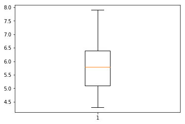

j.Scatter plot

#R
plot(iris$widthOfSepal,iris$lengthOfSepal)

#Python
import matplotlib.pyplot as plt
import sklearn as sklearn
import pandas as pd
from sklearn import datasets
data = datasets.load_iris()
# Convert to Pandas dataframe
iris = pd.DataFrame(data.data, columns=data.feature_names)
img=plt.scatter(iris['sepal width (cm)'],iris['sepal length (cm)'])
#plt.show(img)

k. Read from csv file

#R
tendulkar= read.csv("tendulkar.csv",stringsAsFactors = FALSE,na.strings=c(NA,"-"))
#Dimensions of dataframe
dim(tendulkar)

## [1] 347  13

names(tendulkar)

##  [1] "X"          "Runs"       "Mins"       "BF"         "X4s"       
##  [6] "X6s"        "SR"         "Pos"        "Dismissal"  "Inns"      
## [11] "Opposition" "Ground"     "Start.Date"

Use pandas.read_csv() for Python

#Python
import pandas as pd
#Read csv
tendulkar= pd.read_csv("tendulkar.csv",na_values=["-"])
print(tendulkar.shape)
print(tendulkar.columns)

## (347, 13)
## Index(['Unnamed: 0', 'Runs', 'Mins', 'BF', '4s', '6s', 'SR', 'Pos',
##        'Dismissal', 'Inns', 'Opposition', 'Ground', 'Start Date'],
##       dtype='object')

l. Clean the dataframe in R and Python.

The following steps are done for R and Python
1.Remove rows with ‘DNB’
2.Remove rows with ‘TDNB’
3.Remove rows with absent
4.Remove the “*” indicating not out
5.Remove incomplete rows with NA for R or NaN in Python
6.Do a scatter plot

#R
# Remove rows with 'DNB'
a <- tendulkar$Runs != "DNB"
tendulkar <- tendulkar[a,]
dim(tendulkar)

## [1] 330  13

# Remove rows with 'TDNB'
b <- tendulkar$Runs != "TDNB"
tendulkar <- tendulkar[b,]

# Remove rows with absent
c <- tendulkar$Runs != "absent"
tendulkar <- tendulkar[c,]
dim(tendulkar)

## [1] 329  13

# Remove the "* indicating not out
tendulkar$Runs <- as.numeric(gsub("\\*","",tendulkar$Runs))
dim(tendulkar)

## [1] 329  13

# Select only complete rows - complete.cases()
c <- complete.cases(tendulkar)
#Subset the rows which are complete
tendulkar <- tendulkar[c,]
dim(tendulkar)

## [1] 327  13

# Do some base plotting - Scatter plot
plot(tendulkar$BF,tendulkar$Runs)

#Python 
import pandas as pd
import matplotlib.pyplot as plt
#Read csv
tendulkar= pd.read_csv("tendulkar.csv",na_values=["-"])
print(tendulkar.shape)
# Remove rows with 'DNB'
a=tendulkar.Runs !="DNB"
tendulkar=tendulkar[a]
print(tendulkar.shape)
# Remove rows with 'TDNB'
b=tendulkar.Runs !="TDNB"
tendulkar=tendulkar[b]
print(tendulkar.shape)
# Remove rows with absent
c= tendulkar.Runs != "absent"
tendulkar=tendulkar[c]
print(tendulkar.shape)
# Remove the "* indicating not out
tendulkar.Runs= tendulkar.Runs.str.replace(r"[*]","")
#Select only complete rows - dropna()
tendulkar=tendulkar.dropna()
print(tendulkar.shape)
tendulkar.Runs = tendulkar.Runs.astype(int)
tendulkar.BF = tendulkar.BF.astype(int)
#Scatter plot
plt.scatter(tendulkar.BF,tendulkar.Runs)

## (347, 13)
## (330, 13)
## (329, 13)
## (329, 13)
## (327, 13)

m.Chaining operations on dataframes

To chain a set of operations we need to use an R package like dplyr. Pandas does this The following operations are done on tendulkar data frame by dplyr for R and Pandas for Python below

Group by ground
Compute average runs in each ground
Arrange in descending order

#R
library(dplyr)
tendulkar1 <- tendulkar %>% group_by(Ground) %>% summarise(meanRuns= mean(Runs)) %>%
         arrange(desc(meanRuns))
head(tendulkar1,10)

## # A tibble: 10 × 2
##           Ground  meanRuns
##                 
## 1         Multan 194.00000
## 2          Leeds 193.00000
## 3  Colombo (RPS) 143.00000
## 4        Lucknow 142.00000
## 5          Dhaka 132.75000
## 6     Manchester  93.50000
## 7         Sydney  87.22222
## 8   Bloemfontein  85.00000
## 9     Georgetown  81.00000
## 10 Colombo (SSC)  77.55556

#Python
import pandas as pd
#Read csv
tendulkar= pd.read_csv("tendulkar.csv",na_values=["-"])
print(tendulkar.shape)
# Remove rows with 'DNB'
a=tendulkar.Runs !="DNB"
tendulkar=tendulkar[a]
# Remove rows with 'TDNB'
b=tendulkar.Runs !="TDNB"
tendulkar=tendulkar[b]
# Remove rows with absent
c= tendulkar.Runs != "absent"
tendulkar=tendulkar[c]
# Remove the "* indicating not out
tendulkar.Runs= tendulkar.Runs.str.replace(r"[*]","")

#Select only complete rows - dropna()
tendulkar=tendulkar.dropna()
tendulkar.Runs = tendulkar.Runs.astype(int)
tendulkar.BF = tendulkar.BF.astype(int)
tendulkar1= tendulkar.groupby('Ground').mean()['Runs'].sort_values(ascending=False)
print(tendulkar1.head(10))

## (347, 13)
## Ground
## Multan           194.000000
## Leeds            193.000000
## Colombo (RPS)    143.000000
## Lucknow          142.000000
## Dhaka            132.750000
## Manchester        93.500000
## Sydney            87.222222
## Bloemfontein      85.000000
## Georgetown        81.000000
## Colombo (SSC)     77.555556
## Name: Runs, dtype: float64

9. Functions

product <- function(a,b){
  c<- a*b
  c
}
product(5,7)

## [1] 35

def product(a,b):
  c = a*b
  return c
  
print(product(5,7))

## 35

Conclusion

Personally, I took to R, much like a ‘duck takes to water’. I found the R syntax very simple and mostly intuitive. R packages like dplyr, ggplot2, reshape2, make the language quite irrestible. R is weakly typed and has only numeric and character types as opposed to the full fledged data types in Python.

Python, has too many bells and whistles, which can be a little bewildering to the novice. It is possible that they may be useful as one becomes more experienced with the language. Also I found that installing Python packages sometimes gives errors with Python versions 2.7 or 3.6. This will leave you scrambling to google to find how to fix these problems. These can be quite frustrating. R on the other hand makes installing R packages a breeze.

Anyway, this is my current opinion, and like all opinions, may change in the course of time. Let’s see!

I may write a follow up post with more advanced features of R and Python. So do keep checking! Long live R! Viva la Python!

Note: This post was created using RStudio’s RMarkdown which allows you to embed R and Python code snippets. It works perfectly, except that matplotlib’s pyplot does not display.

Also see
1. My book ‘Deep Learning from first principles:Second Edition’ now on Amazon
2. Dabbling with Wiener filter using OpenCV
3. My book ‘Practical Machine Learning in R and Python: Third edition’ on Amazon
4. Design Principles of Scalable, Distributed Systems
5. Re-introducing cricketr! : An R package to analyze performances of cricketers
6. Natural language processing: What would Shakespeare say?
7. Brewing a potion with Bluemix, PostgreSQL, Node.js in the cloud
8. Simulating an Edge Shape in Android
To see all posts click Index of posts

The common alphabet of programming languages

“All animals are equal, but some animals are more equal than other.” “Four legs good, two legs bad.”

from Animal Farm by George Orwell

Note: This post is largely intended for those who are embarking on their journey into the world of programming. The article below highlights a set of constructs that recur in many imperative, dynamic and object-oriented languages. While these constructs cannot be applied directly to functional programming languages like Lisp,Haskell or Clojure, it may help. To some extent the programming language domain has been intentionally oversimplified to show that languages are not as daunting as they seem. Clearly there are a lot more subtle and complex differences among languages. Hope you have fun programming!

Introduction: Anybody who is about to venture into the deep waters of programming will be bewildered and awed by the almost limitless number of programming languages and the associated paradigms on which they are based on. It is easy to feel apprehensive of programming, when faced with this this array of languages, not to mention the seemingly quirky syntax of each language. Many opinions abound, about what is the best programming language. In my opinion each language is best suited for a particular class of problems and is usually clunky if used outside of this. As an aside here is an interesting link provided by reader AKS to Rosetta Code, which is stated to be a a programming chrestomathy (present solutions to the same task in as many different languages as possible, to demonstrate how languages are similar and different, and to aid a person with a grounding in one approach to a problem in learning another. Rosetta Code currently has 772 tasks, 165 draft tasks, and is aware of 582 languages)

You are likely to hear “All programming languages are equal, but some languages are more equal than others” from seasoned programmers who have their own pet language. There may also be others who swear that “procedural languages good, object oriented languages bad” or maybe “object oriented languages good, aspect oriented languages bad”. Unity in diversity Regardless of the language this post discusses a thread that is common to all programming languages. In fact any programming language can be expressed as

Lx = C + Sx

Where Lx is any programming language ‘x’. All programming languages have a set of core, common constructs which I have denoted as ‘C’ and a set of Specialized constructs, unique to each language ‘x’ which I have denoted as Sx. I would like to look at these constructs that are common to most programming languages like C,C++,Perl, Python, Ruby, C#, R, Octave etc. In my opinion knowing these core, common constructs and a few of the more specialized constructs should allow you to get started off in the language of your choice. You can pick up the more unique constructs as you go along. Here are the common constructs (C mentioned above) that you must familiarize yourself with when embarking on a new language

Reading user input and printing to screen
Reading and writing from a file
Conditional statement if-then-else if-else
Loops – For, while, repeat, do while etc.

Knowing these constructs and some of the basic concepts unique to each language for e.g.
– Structure, Pointers in C,
– Classes, inheritance in C++
– Subsetting in Octave, R
– car, cdr in Lisp will enable you to get started off in your chosen language.
I show the examples of these core constructs in many languages. Note the similarity between these constructs
1. C
Read from and write to console
scanf(x,”%d); printf(“The value of x is %d”, x);
Read from and write to filefread(buffer, strlen(c)+1, 1, fp); fwrite(c, strlen(c) + 1, 1, fp);

Conditional
if(x > 5) { printf(“x is greater than 5”); } else if (x < 5) { printf(“x is less than 5”); } else{ printf(“x is equal to 5”); }
Loops I will only consider for loops, though one could use while, repeat etC.
for(i =0; i <100; i++) { money = money++) }
2. C++
Read from and write to console
cin >> age; Cout << “The value is “ << value

Read from and write to a file // open a file in read mode.
ifstream infile; infile.open("afile.dat"); cout << "Reading from the file" << endl; infile >> data; ofstream outfile; outfile.open("afile.dat"); // write inputted data into the file. outfile << data << endl;
Conditional same as C
if(x > 5) { printf(“x is greater than 5”); }
else if (x < 5) { printf(“x is less than 5”); } else{ printf(“x is equal to 5”); }
Loops
for(i =0; i <100; i++) { money = money++)

}

2. C++ Read from and write to console
cin >> age;
Cout << “The value is “ << value
Read from and write to a file // open a file in read mode.
ifstream infile;
infile.open("afile.dat");
cout << "Reading from the file" << endl;
infile >> data; ofstream outfile;
outfile.open("afile.dat");
// write inputted data into the file.
outfile << data << endl;
Conditional same as C
if(x > 5) {
printf(“x is greater than 5”);
}
else if (x < 5) {
printf(“x is less than 5”);
}
else{ printf(“x is equal to 5”);
}
Loops
for(i =0; i <100; i++){
money = money++)
}
3. Java
Reading from and writing to standard input
Console c = System.console();
int val = c.readLine("Enter a value: ");
System.out.println("Value is "+ val);
Reading and writing from file
try {
in = new FileInputStream("input.txt");
out = new FileOutputStream("output.txt");
int c;
while ((c = in.read()) != -1) {
out.write(c); } } ...
Conditional (same as C)
if(x > 5) {
printf(“x is greater than 5”);
}
else if (x < 5) {
printf(“x is less than 5”);
}
else{ printf(“x is equal to 5”); }
Loops (same as C)
for(i =0; i <100; i++){
money = money++)
}

4. Perl Read from console
#!/usr/bin/perl
$userinput = ;
chomp ($userinput);
Write to console
print "User typed $userinput\n";
Reading and write to a file
open(IN,"infile") || die "cannot open input file";
open(OUT,"outfile") || die "cannot open output file";
while() {
print OUT $_;
# echo line read
}
close(IN);
close(OUT)
Conditional
if( $a == 20 ){
# if condition is true then print the following
printf "a has a value which is 20\n";
}
elsif( $a == 30 ){
# if condition is true then print the following
printf "a has a value which is 30\n";
}else{
# if none of the above conditions is true
printf "a has a value which is $a\n";
}
Loops
for (my $i=0; $i <= 9; $i++) {
print "$i\n";
}

5. Lisp
The syntax for Lisp will be different from the others as it is a functional language. You need to familiarize yourself with these constructs to move ahead
Read and write to console
To read from standard input use
(let ((temp 0))
(print ‘(Enter temp))
(setf temp (read))
(print (append ‘(the temp is) (list temp))))
Read from and write to file
(with-open-file (stream “C:\\acl82express\\lisp\\count.cl”)
(do ((line (read-line stream nil) (read-line stream nil)))
(with-open-file (stream “C:\\acl82express\\lisp\\test.txt” :direction :output :if-exists :supersede)
(write-line “test” stream) nil)
Conditional
$ (cond ((< x 5)
(setf x (+ x 8))
(setf y (* 2 y)))
((= x 10) (setf x (* x 2)))
(t (setf x 8)))
Loops
$ (setf x 5)
$ (let ((i 0))
(loop (setf y (* x i))
(when (> i 10) (return))
(print i) (prin1 y) (incf i )))

6. Python
Reading and writing from console
var = raw_input("Please enter something: ")
print “You entered: ” value
Reading and writing from files
f = open(filename, 'r')
a = f.readline().strip()
target = open(filename, 'w')
target.write(line1)
Conditionals
if x > 5:
print "x is greater than 5”
elif
x < 5:
print "x is less than 5"
else:
print "x is equal to 5"
Loops
for i in range(0, 6):
print "Value is :" % i 7.

R
x=5
paste('The value of x is =',x)
Reading and writing to a file
infile = read.csv(“file”)
write(x, file = "data", sep = " ")
Conditional
if(x > 5){
print(“x is greater than 5”)
}else if(x < 5){
print(“x is less than 5”)
}else {
print(“x is equal to 5”)
}
Loops
for (i in 1:10) print(i)

Conclusion
As can be seen the core constructs are very similar in different languages save for some minor variations. It is generally useful to get started with just knowing these constructs and few other important other features of the language that you are trying to learn. It is possible to code most programs with these Core constructs and a few of the Specialized constructs in the language. These Core constructs are the glue that hold your code together.

You can learn more compact and more powerful features of the language as you go along The above core constructs are like the letters of the programming language alphabet. You need to construct words by stringing together these constructs and form sensible sentences which will be your program. Good luck with your adventure in your next new programming language!!!

Also see
1.Programming languages in layman’s language
2. The mind of the programmer
3. How to program – Some essential tips
4. Programming Zen and now – Some essential tips -2

Bend it like Bluemix, MongoDB using Auto-scaling – Part 2!

This post takes off from my previous post Bend it like Bluemix, MongoDB using Auto-scale – Part 1! In this post I generate traffic using Multi-Mechanize a performance test framework and check out the auto-scaling on Bluemix, besides also doing some rudimentary check on the latency and throughput for this test application. In this particular post I generate concurrent threads which insert documents into MongoDB.

Note: As mentioned in my earlier post this is more of a prototype and the typical situation when architecting cloud applications. Clearly I have not optimized my cloud app (bluemixMongo) for maximum efficiency. Also this a simple 2 tier application with a rudimentary Web interface and a NoSQL DB at This is more of a Proof of Concept (PoC) for the auto-scaling service on Bluemix.

As earlier mentioned the bluemixMongo app is a modification of my earlier post Spicing up a IBM Bluemix cloud app with MongoDB and NodeExpress. The bluemixMongo cloud app that was used for this auto-scaling test can be forked from Devops at bluemixMongo or from GitHib at bluemix-mongo-autoscale. The Multi-mechanize config file, scripts and results can be found at GitHub in multi-mechanize

The document to be inserted into MongoDB consists of 3 fields – Firstname, Lastname and Mobile. To simulate the insertion of records into MongoDB I created a Multi-Mechanize script that will generate random combination of letters and numbers for the First and Last names and a random 9 digit number for the mobile. The code for this script is shown below

1. The snippet below measure the latency for loading the ‘New User’ page

v_user.py
def run(self): # create a Browser instance br = mechanize.Browser() # don"t bother with robots.txt br.set_handle_robots(False) print("Rendering new user") br.addheaders = [("User-agent", "Mozilla/5.0Compatible")] # start the timer start_timer = time.time() # submit the request resp = br.open("http://bluemixmongo.mybluemix.net/newuser") #resp = br.open("http://localhost:3000/newuser") resp.read() # stop the timer latency = time.time() - start_timer # store the custom timer self.custom_timers["Load Add User Page"] = latency # think-time time.sleep(2)

The script also measures the time taken to submit the form containing the Firstname, Lastname and Mobile

# select first (zero-based) form on page br.select_form(nr=0) # Create random Firstname a = (''.join(random.choice(string.ascii_uppercase) for i in range(5))) b = (''.join(random.choice(string.digits) for i in range(5))) firstname = a + b # Create random Lastname a = (''.join(random.choice(string.ascii_uppercase) for i in range(5))) b = (''.join(random.choice(string.digits) for i in range(5))) lastname = a + b # Create a random mobile number mobile = (''.join(random.choice(string.digits) for i in range(9))) # set form field br.form["firstname"] = firstname br.form["lastname"] = lastname br.form["mobile"] = mobile # start the timer start_timer = time.time() # submit the form resp = br.submit() print("Submitted.") resp.read() # stop the timer latency = time.time() - start_timer # store the custom timer self.custom_timers["Add User"] = latency

2. The config.cfg file is setup to generate 2 asynchronous thread pools of 10 threads for about 400 seconds

config.cfg
run_time = 400 rampup = 0 results_ts_interval = 10 progress_bar = on console_logging = off xml_report = off [user_group-1] threads = 10 script = v_user.py [user_group-2] threads = 10 script = v_user.py

3. The code to add a new user in the app (adduser.js) uses the ‘async’ Node module to enforce sequential processing.

adduser.js
async.series([ function(callback) { collection = db.collection('phonebook', function(error, response) { if( error ) { return; // Return immediately } else { console.log("Connected to phonebook"); } }); callback(null, 'one'); }, function(callback) // Insert the record into the DB collection.insert({ "FirstName" : FirstName, "LastName" : LastName, "Mobile" : Mobile }, function (err, doc) { if (err) { // If it failed, return error res.send("There was a problem adding the information to the database."); } else { // If it worked, redirect to userlist - Display users res.location("userlist"); // And forward to success page res.redirect("userlist") } }); collection.find().toArray(function(err, items) { console.log("**************************>>>>>>>Length =" + items.length); db.close(); // Make sure that the open DB connection is close }); callback(null, 'two'); } ]);

4. To checkout auto-scaling the instance memory was kept at 128 MB. Also the scale-up policy was memory based and based on the memory of the instance exceeding 55% of 128 MB for 120 secs. The scale up based on CPU utilization was to happen when the utilization exceed 80% for 300 secs.

5. Check the auto-scaling policy

6. Initially as seen there is just a single instance

7. At around 48% of the script with around 623 transactions the instance is increased by 1. Note that the available memory is decreased by 640 MB – 128 MB = 512 MB.

8. At around 1324 transactions another instance is added

Note: Bear in mind

a) The memory threshold was artificially brought down to 55% of 128 MB.b) The app itself is not optimized for maximum efficiency

9. The Metric Statistics tab for the Autoscaling service shows this memory breach and the trigger for autoscaling

10. The Scaling history Tab for the Auto-scaling service displays the scale-up and scale-down and the policy rules based on which the scaling happened

11. If you go to the results folder for the Multi-mechanize tool the response and throughput are captured.

The multi-mechanize commands are executed as follows
To create a new project
multimech-newproject.exe adduser
This will create 2 folders a) results b) test_scripts and the file c) config.cfg. The v_user.py needs to be updated as required

To run the script
multimech-run.exe adduser

12.The results are shown below

a) Load Add User page (Latency)