Convolutional Neural Networks (CNNs), have been very popular in the last decade or so. CNNs have been used in multiple applications like image recognition, image classification, facial recognition, neural style transfer etc. CNN’s have been extremely successful in handling these kind of problems. How do they work? What makes them so successful? What is the principle behind CNN’s ?
Note: this post is based on two Coursera courses I did, namely namely Deep Learning specialisation by Prof Andrew Ng and Tensorflow Specialisation by Laurence Moroney.
In this post I show you how CNN’s work. To understand how CNNs work, we need to understand the concept behind machine learning algorithms. If you take a simple machine learning algorithm in which you are trying to do multi-class classification using softmax or binary classification with the sigmoid function, for a set of for a set of input features against a target variable we need to create an objective function of the input features versus the target variable. Then we need to minimise this objective function, while performing gradient descent, such that the cost is the lowest. This will give the set of weights for the different variables in the objective function.
The central problem in ML algorithms is to do feature selection, i.e. we need to find the set of features that actually influence the target. There are various methods for doing features selection – best fit, forward fit, backward fit, ridge and lasso regression. All these methods try to pick out the predictors that influence the output most, by making the weights of the other features close to zero. Please look at my post – Practical Machine Learning in R and Python – Part 3, where I show you the different methods for doing features selection.
In image classification or Image recognition we need to find the important features in the image. How do we do that? Many years back, have played around with OpenCV. While working with OpenCV I came across are numerous filters like the Sobel ,the Laplacian, Canny, Gaussian filter et cetera which can be used to identify key features of the image. For example the Canny filter feature can be used for edge detection, Gaussian for smoothing, Sobel for determining the derivative and we have other filters for detecting vertical or horizontal edges. Take a look at my post Computer Vision: Ramblings on derivatives, histograms and contours So for handling images we need to apply these filters to pick out the key features of the image namely the edges and other features. So rather than using the entire image’s pixels against the target class we can pick out the features from the image and use that as predictors of the target output.

Note: that in Convolutional Neural Network, fixed filter values like the those shown above are not used directly. Rather the filter values are learned through back propagation and gradient descent as shown below.
In CNNs the filter values are considered to be weights which are then learned and updated in each forward/backward propagation cycle much like the way a fully connected Deep Learning Network learns the weights of the network.
Here is a short derivation of the most important parts of how a CNNs work
The convolution of a filter F with the input X can be represented as.

Convolving we get

This the forward propagation as it passes through a non-linear function like Relu

To go through back propagation we need to compute the 

The loss with respect to the output is 


We need these local derivatives because we can learn the filter values using gradient descent

where 

In the fully connected layers the weights associated with each connection is computed in every cycle of forward and backward propagation using gradient descent. Similarly, the filter values are also computed and updated in each forward and backward propagation cycle. This is done so as to minimize the loss at the output layer.
By using the chain rule and simplifying the back propagation for the Convolutional layers we get these 2 equations. The first equation is used to learn the filter values and the second is used pass the loss to layers before
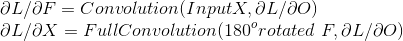
(for the detailed derivation see Convolutions and Backpropagations
An important aspect of performing convolutions is to reduce the size of the flattened image that is passed into the fully connected DL network. Successively convolving with 2D filters and doing a max pooling helps to reduce the size of the features that we can use for learning the images. Convolutions also enable a sparsity of connections as you can see in the diagram below. In the LeNet-5 Convolution Neural Network of Yann Le Cunn, successive convolutions reduce the image size from 28 x 28=784 to 120 flattened values.

Here is an interesting Deep Learning problem. Convolutions help in picking out important features of images and help in image classification/ detection. What would be its equivalent if we wanted to identify the Carnatic ragam of a song? A Carnatic ragam is roughly similar to Western scales (major, natural, melodic, blues) with all its modes Lydian, Aeolion, Phyrgian etc. Except in the case of the ragams, it is more nuanced, complex and involved. Personally, I can rarely identify a ragam on which a carnatic song is based (I am tone deaf when it comes to identifying ragams). I have come to understand that each Carnatic ragam has its own character, which is made up of several melodic phrases which are unique to that flavor of a ragam. What operation like convolution would be needed so that we can pick out these unique phrases in a Carnatic ragam? Of course, we would need to use it in Recurrent Neural Networks with LSTMs as a song is a time sequence of notes to identify sequences. Nevertheless, if there was some operation with which we can pick up the distinct, unique phrases from a song and then run it through a classifier, maybe we would be able to identify the ragam of the song.
Below I implement 3 simple CNN using the Dogs vs Cats Dataset from Kaggle. The first CNN uses regular Convolutions a Fully connected network to classify the images. The second approach uses Image Augmentation. For some reason, I did not get a better performance with Image Augumentation. Thirdly I use the pre-trained Inception v3 network.
1. Basic Convolutional Neural Network in Tensorflow & Keras
You can view the Colab notebook here – Cats_vs_dogs_1.ipynb
Here some important parts of the notebook
Create CNN Model
- Use 3 Convolution + Max pooling layers with 32,64 and 128 filters respectively
- Flatten the data
- Have 2 Fully connected layers with 128, 512 neurons with relu activation
- Use sigmoid for binary classification
model = tf.keras.models.Sequential([
    tf.keras.layers.Conv2D(32,(3,3),activation='relu',input_shape=(150,150,3)),
    tf.keras.layers.MaxPooling2D(2,2),
    tf.keras.layers.Conv2D(64,(3,3),activation='relu'),
    tf.keras.layers.MaxPooling2D(2,2),
    tf.keras.layers.Conv2D(128,(3,3),activation='relu'),
    tf.keras.layers.MaxPooling2D(2,2),
    tf.keras.layers.Flatten(),
    tf.keras.layers.Dense(128,activation='relu'),
    tf.keras.layers.Dense(512,activation='relu'),
    tf.keras.layers.Dense(1,activation='sigmoid')
])
Print model summary
model.summary()
Use the Adam Optimizer with binary cross entropy
model.compile(optimizer='adam',
             loss='binary_crossentropy',
             metrics=['accuracy'])
Perform Gradient Descent
- Do Gradient Descent for 15 epochs
history=model.fit(train_generator,
                 validation_data=validation_generator,
                 steps_per_epoch=100,
                 epochs=15,
                 validation_steps=50,
                 verbose=2)
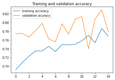
Plot results
-
- Plot training and validation accuracy
- Plot training and validation loss
#-----------------------------------------------------------
# Retrieve a list of list results on training and test data
# sets for each training epoch
#-----------------------------------------------------------
acc      = history.history[     'accuracy' ]
val_acc  = history.history[ 'val_accuracy' ]
loss     = history.history[    'loss' ]
val_loss = history.history['val_loss' ]

epochs   = range(len(acc)) # Get number of epochs

#------------------------------------------------
# Plot training and validation accuracy per epoch
#------------------------------------------------
plt.plot  ( epochs,     acc,label="training accuracy" )
plt.plot  ( epochs, val_acc, label='validation acuracy' )
plt.title ('Training and validation accuracy')
plt.legend()

plt.figure()

#------------------------------------------------
# Plot training and validation loss per epoch
#------------------------------------------------
plt.plot  ( epochs,     loss , label="training loss")
plt.plot  ( epochs, val_loss,label="validation loss" )
plt.title ('Training and validation loss'   )
plt.legend()


2. CNN with Image Augmentation
You can check the Cats_vs_Dogs_2.ipynb
Including the important parts of this implementation below
Use Image Augumentation
Use Image Augumentation to improve performance
- Use the same model parameters as before
- Perform the following image augmentation
- width, height shift
- shear and zoom
Note: Adding rotation made the performance worse
import tensorflow as tf
from tensorflow import keras
from tensorflow.keras.optimizers import RMSprop
from tensorflow.keras.preprocessing.image import ImageDataGenerator
model = tf.keras.models.Sequential([
    tf.keras.layers.Conv2D(32,(3,3),activation='relu',input_shape=(150,150,3)),
    tf.keras.layers.MaxPooling2D(2,2),
    tf.keras.layers.Conv2D(64,(3,3),activation='relu'),
    tf.keras.layers.MaxPooling2D(2,2),
    tf.keras.layers.Conv2D(128,(3,3),activation='relu'),
    tf.keras.layers.MaxPooling2D(2,2),
    tf.keras.layers.Flatten(),
    tf.keras.layers.Dense(128,activation='relu'),
    tf.keras.layers.Dense(512,activation='relu'),
    tf.keras.layers.Dense(1,activation='sigmoid')
])


train_datagen = ImageDataGenerator(
      rescale=1./255,
      #rotation_range=90,
      width_shift_range=0.2,
      height_shift_range=0.2,
      shear_range=0.2,
      zoom_range=0.2)
      #horizontal_flip=True,
      #fill_mode='nearest')

validation_datagen = ImageDataGenerator(rescale=1./255)
#
train_generator = train_datagen.flow_from_directory(train_dir,
                                                    batch_size=32,
                                                    class_mode='binary',
                                                    target_size=(150, 150))
# --------------------
# Flow validation images in batches of 20 using test_datagen generator
# --------------------
validation_generator =  validation_datagen.flow_from_directory(validation_dir,
                                                         batch_size=32,
                                                         class_mode  = 'binary',
                                                         target_size = (150, 150))

# Use Adam Optmizer
model.compile(optimizer='adam',
             loss='binary_crossentropy',
             metrics=['accuracy'])
Perform Gradient Descent
history=model.fit(train_generator,
                 validation_data=validation_generator,
                 steps_per_epoch=100,
                 epochs=15,
                 validation_steps=50,
                 verbose=2)
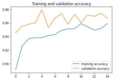
Plot results
- Plot training and validation accuracy
- Plot training and validation loss
import matplotlib.pyplot as plt
#-----------------------------------------------------------
# Retrieve a list of list results on training and test data
# sets for each training epoch
#-----------------------------------------------------------
acc      = history.history[     'accuracy' ]
val_acc  = history.history[ 'val_accuracy' ]
loss     = history.history[    'loss' ]
val_loss = history.history['val_loss' ]

epochs   = range(len(acc)) # Get number of epochs

#------------------------------------------------
# Plot training and validation accuracy per epoch
#------------------------------------------------
plt.plot  ( epochs,     acc,label="training accuracy" )
plt.plot  ( epochs, val_acc, label='validation acuracy' )
plt.title ('Training and validation accuracy')
plt.legend()

plt.figure()

#------------------------------------------------
# Plot training and validation loss per epoch
#------------------------------------------------
plt.plot  ( epochs,     loss , label="training loss")
plt.plot  ( epochs, val_loss,label="validation loss" )
plt.title ('Training and validation loss'   )
plt.legend()

Implementation using Inception Network V3
The implementation is in the Colab notebook Cats_vs_Dog_3.ipynb
This is implemented as below
Use Inception V3
import os

from tensorflow.keras import layers
from tensorflow.keras import Model


from tensorflow.keras.applications.inception_v3 import InceptionV3
pre_trained_model = InceptionV3(input_shape = (150, 150, 3),
                                include_top = False,
                                weights = 'imagenet')


for layer in pre_trained_model.layers:
  layer.trainable = False

# pre_trained_model.summary()

last_layer = pre_trained_model.get_layer('mixed7')
print('last layer output shape: ', last_layer.output_shape)
last_output = last_layer.output
Use Layer 7 of Inception Network
- Use Image Augumentation
- Use Adam Optimizer
import tensorflow as tf
from tensorflow import keras
from tensorflow.keras.optimizers import RMSprop
from tensorflow.keras.preprocessing.image import ImageDataGenerator
# Flatten the output layer to 1 dimension
x = layers.Flatten()(last_output)
# Add a fully connected layer with 1,024 hidden units and ReLU activation
x = layers.Dense(1024, activation='relu')(x)
# Add a dropout rate of 0.2
x = layers.Dropout(0.2)(x)
# Add a final sigmoid layer for classification
x = layers.Dense  (1, activation='sigmoid')(x)

model = Model( pre_trained_model.input, x)
#train_datagen = ImageDataGenerator( rescale = 1.0/255. )
#validation_datagen = ImageDataGenerator( rescale = 1.0/255. )

train_datagen = ImageDataGenerator(
      rescale=1./255,
      #rotation_range=90,
      width_shift_range=0.2,
      height_shift_range=0.2,
      shear_range=0.2,
      zoom_range=0.2)
      #horizontal_flip=True,
      #fill_mode='nearest')

validation_datagen = ImageDataGenerator(rescale=1./255)
#
train_generator = train_datagen.flow_from_directory(train_dir,
                                                    batch_size=32,
                                                    class_mode='binary',
                                                    target_size=(150, 150))
# --------------------
# Flow validation images in batches of 20 using test_datagen generator
# --------------------
validation_generator =  validation_datagen.flow_from_directory(validation_dir,
                                                         batch_size=32,
                                                         class_mode  = 'binary',
                                                         target_size = (150, 150))


model.compile(optimizer='adam',
             loss='binary_crossentropy',
             metrics=['accuracy'])
Fit model
history=model.fit(train_generator,
                 validation_data=validation_generator,
                 steps_per_epoch=100,
                 epochs=15,
                 validation_steps=50,
                 verbose=2)
Plot results
- Plot training and validation accuracy
- Plot training and validation loss
import matplotlib.pyplot as plt
#-----------------------------------------------------------
# Retrieve a list of list results on training and test data
# sets for each training epoch
#-----------------------------------------------------------
acc      = history.history[     'accuracy' ]
val_acc  = history.history[ 'val_accuracy' ]
loss     = history.history[    'loss' ]
val_loss = history.history['val_loss' ]

epochs   = range(len(acc)) # Get number of epochs

#------------------------------------------------
# Plot training and validation accuracy per epoch
#------------------------------------------------
plt.plot  ( epochs,     acc,label="training accuracy" )
plt.plot  ( epochs, val_acc, label='validation acuracy' )
plt.title ('Training and validation accuracy')
plt.legend()

plt.figure()

#------------------------------------------------
# Plot training and validation loss per epoch
#------------------------------------------------
plt.plot  ( epochs,     loss , label="training loss")
plt.plot  ( epochs, val_loss,label="validation loss" )
plt.title ('Training and validation loss'   )
plt.legend()

I intend to do some interesting stuff with Convolutional Neural Networks.
Watch this space!
See also
1. Architecting a cloud based IP Multimedia System (IMS)
2. Exploring Quantum Gate operations with QCSimulator
3. Big Data 6: The T20 Dance of Apache NiFi and yorkpy
4. The Many Faces of Latency
5. The Clash of the Titans in Test and ODI cricket
To see all posts click Index of posts

 Checkout my book ‘Deep Learning from first principles: Second Edition – In vectorized Python, R and Octave’. My book starts with the implementation of a simple 2-layer Neural Network and works its way to a generic L-Layer Deep Learning Network, with all the bells and whistles. The derivations have been discussed in detail. The code has been extensively commented and included in its entirety in the Appendix sections. My book is available on Amazon as


 Checkout my book ‘Deep Learning from first principles: Second Edition – In vectorized Python, R and Octave’. My book starts with the implementation of a simple 2-layer Neural Network and works its way to a generic L-Layer Deep Learning Network, with all the bells and whistles. The derivations have been discussed in detail. The code has been extensively commented and included in its entirety in the Appendix sections. My book is available on Amazon as


 Checkout my book ‘Deep Learning from first principles: Second Edition – In vectorized Python, R and Octave’. My book starts with the implementation of a simple 2-layer Neural Network and works its way to a generic L-Layer Deep Learning Network, with all the bells and whistles. The derivations have been discussed in detail. The code has been extensively commented and included in its entirety in the Appendix sections. My book is available on Amazon as


 by doing
 .
.
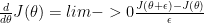
 be a function that computes the derivative
  . Gradient Checking allows us to numerically evaluate the implementation of the function
 as opposed
  for the 1-sided derivative.
 by bumping up
  (
( )
)
 by bumping down

 or ‘gradapprox’ as
 using the 2 sided derivative.
 or
or  the implementation is correct. In the
  – 0.9
– 0.9 – 0.9
– 0.9 and
and 
 then we we can represent the exponentially average value at time ‘t’ as a sequence of the the previous value
  and
and  as shown below
 represent the average of the data set over
  By choosing different values of


 , which is an exponentially decaying function.


 where
where and
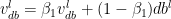
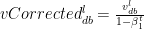
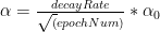
and  are the momentum terms which are exponentially weighted with the corresponding gradients ‘dW’ and ‘db’ at the corresponding layer ‘l’ The code snippet for Stochastic Gradient Descent with momentum in R is shown below


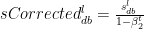
 and
and  are the RMSProp terms which are exponentially weighted with the corresponding gradients ‘dW’ and ‘db’ at the corresponding layer ‘l’