I am late to the ‘Win probability’ computation for T20 matches, but managed to jump on to this bus with this post. Win Probability analysis and computation have been around for some time and are used in baseball, NFL, soccer hockey and others. On T20 cricket, the following posts from White Ball Analytics & Sports Data Science were good pointers to the general approach. The data for the Win Probability computation is taken from Cricsheet.
My initial Machine Learning models could not do better than 62% accuracy. I created a data set of ~830 IPL matches which roughly came to about 280,000 rows of ball-by-ball match data but I could not move beyond 62%. Addition of T20 men moved the needle to 64% accuracy. I spent time tuning Deep Learning networks using Tensorflow and Keras. Finally, I added T20 data from 9 T20 leagues – IPL, T20 men, T20 women, BBL, CPL, NTB, PSL, WBB, SSM. I had one large data set of 1.2 million rows of ball by ball data. The data frame looks like

I created a data frame for each match from ball Num 1 to ballNum ~240 for the 1st and 2nd innings of the match. My initial set of features were ballNum, runs, runRate, numWickets. The target variable isWinner= {0,1} depending on whether the team has won or lost the match.
The features
- ballNum – ball number for 1 ~ 240+ in data frame. 1 – 120+ for 1st innings and 120+ – 240+ in 2nd innings including noballs, wides etc.
- runs = cumulative runs scored at the ball count
- runRate = cumulative runs scored/ ballNum (for 1st innings) and runs= required runs/ball Num for 2nd innings
- numWickets = wickets lost
The target variable isWinner can take values {0,1} depending whether the team won or lost
With this initial dataframe, even though I had close to 1.2 million rows of ball by ball data of T20 matches my best performance with vanilla Logistic regression & SVM in Python was about 64% accuracy.
# Read all the data from 9 T20 leagues
# BBL,CPL, IPL, NTB, PSL, SSM, T20 Men, T20 Women, WBB
df1=pd.read_csv('matchesT20M.csv')
df2=pd.read_csv('matchesIPL.csv')
df3=pd.read_csv('matchesBBL.csv')
df4=pd.read_csv('matchesCPL.csv')
df5=pd.read_csv('matchesNTB.csv')
df6=pd.read_csv('matchesPSL.csv')
df7=pd.read_csv('matchesSSM.csv')
df8=pd.read_csv('matchesT20W.csv')
df9=pd.read_csv('matchesWBB.csv')

# Create one large dataframe
df10=pd.concat([df1,df2,df3,df4,df5,df6,df7,df8,df9])
print("Shape of dataframe=",df10.shape)
print("#####################################")
stats=check_values(df10)
print("#####################################")
model_fit(df10)
#norm_model_fit(df,stats)
svm_model_fit(df10)

Shape of dataframe= (1206901, 6)
#####################################
Null values: False
It contains 0 infinite values

Accuracy of Logistic regression classifier on training set: 0.63
Accuracy of Logistic regression classifier on test set: 0.64
Accuracy: 0.64
Precision: 0.62
Recall: 0.65
F1: 0.64


Accuracy of Linear SVC classifier on training set: 0.52
Accuracy of Linear SVC classifier on test set: 0.52
With Tensorflow/Keras the performance was about 67%. I tried several things
- Normalisation
- Tried different learning rates
- Different optimisers – SGD, RMSProp, Adam
- Changed depth and width of Neural Network
However I did not get much improvement. Finally I decided to do some Feature engineering. I added 2 new features
a) Runs Momentum : This feature is based on the fact that more the wickets in hand, the more freely the batsmen can make risky strokes, hence increasing the momentum of the runs, This is calculated as
runsMomentum = (11 – numWickets)/balls remaining
b) Performance Index: This feature is the product of the run rate x wickets in hand. In other words, if the strike rate is good and fewer wickets lost at the point in the match, then the performance index is higher at that point in the match will be higher
The final set of features chosen were as below

I had also included the balls Remaining in the innings. Now with this set of features I decided to execute Tensorflow/Keras and do a GridSearch with different learning rates, optimisers. After a couple of hours of computation I got an accuracy of 0.73. I needed to be able to read the ML model in R which required installation of Tensorflow, reticulate and Keras in RStudio and I had several issues. Since I hit a roadblock I moved to regular R models
I performed WIn Probability computation in the following ways
A) Win Probability with Vanilla Logistic Regression (R)
With vanilla Logistic Regression in R using the ‘glm’ package I got an accuracy of 0.67, sensitivity of 0.68 and specificity of 0.65 as shown below
library(dplyr)
library(caret)
library(e1071)
library(ggplot2)

# Read all the data from 9 T20 leagues
# BBL,CPL, IPL, NTB, PSL, SSM, T20 Men, T20 Women, WBB
df1=read.csv("output2/matchesBBL2.csv")
df2=read.csv("output2/matchesCPL2.csv")
df3=read.csv("output2/matchesIPL2.csv")
df4=read.csv("output2/matchesNTB2.csv")
df5=read.csv("output2/matchesPSL2.csv")
df6=read.csv("output2/matchesSSM2.csv")
df7=read.csv("output2/matchesT20M2.csv")
df8=read.csv("output2/matchesT20W2.csv")
df9=read.csv("output2/matchesWBB2.csv")

# Create one large dataframe
df=rbind(df1,df2,df3,df4,df5,df6,df7,df8,df9)

# Helper function to split into training/test
trainTestSplit <- function(df,trainPercent,seed1){
  ## Sample size percent
  samp_size <- floor(trainPercent/100 * nrow(df))
  ## set the seed
  set.seed(seed1)
  idx <- sample(seq_len(nrow(df)), size = samp_size)
  idx

}

train_idx <- trainTestSplit(df,trainPercent=80,seed=5)
train <- df[train_idx, ]

test <- df[-train_idx, ]
# Fit a generalized linear logistic model,
fit=glm(isWinner~.,family=binomial,data=train,control = list(maxit = 50))

a=predict(fit,newdata=train,type="response")
# Set response >0.5 as 1 and <=0.5 as 0
b=as.factor(ifelse(a>0.5,1,0))
# Compute the confusion matrix for training data

confusionMatrix(
  factor(b, levels = 0:1),
  factor(train$isWinner, levels = 0:1)
)

Confusion Matrix and Statistics

          Reference
Prediction
  0      1
         0 339938 160336
         1 154236 310217

               Accuracy : 0.6739
                 95% CI : (0.673, 0.6749)
    No Information Rate : 0.5122
    P-Value [Acc > NIR] : < 2.2e-16

                  Kappa : 0.3473

 Mcnemar's Test P-Value : < 2.2e-16

            Sensitivity : 0.6879
            Specificity : 0.6593
         Pos Pred Value : 0.6795
         Neg Pred Value : 0.6679
             Prevalence : 0.5122
         Detection Rate : 0.3524
   Detection Prevalence : 0.5186
      Balanced Accuracy : 0.6736

       'Positive' Class : 0

# This can be saved and loaded as
saveRDS(fit, "glm.rds")
ml_model <- readRDS("glm.rds")
Using the above ML model on Deccan Chargers vs Chennai Super on 27-04-2009 the Win Probability as the match progresses is as below

The Worm wicket graph of this match shows it was a closely fought match

B) Win Probability using Random Forests with Tidy Models – R
Initially I tried Tidy models with tuning for glmnet. The best I got was 0.67. However, I got an excellent performance using TidyModels with Random Forests. I am using Tidy Models for the first time and I have been blown away with how logically it is constructed, much like dplyr & ggplot2.
library(dplyr)
library(caret)
library(e1071)
library(ggplot2)
library(tidymodels)

# Helper packages
library(readr)       # for importing data
library(vip)
library(ranger)
# Read all the data from 9 T20 leagues
# BBL,CPL, IPL, NTB, PSL, SSM, T20 Men, T20 Women, WBB

df1=read.csv("output2/matchesBBL2.csv")
df2=read.csv("output2/matchesCPL2.csv")
df3=read.csv("output2/matchesIPL2.csv")
df4=read.csv("output2/matchesNTB2.csv")
df5=read.csv("output2/matchesPSL2.csv")
df6=read.csv("output2/matchesSSM2.csv")
df7=read.csv("output2/matchesT20M2.csv")
df8=read.csv("output2/matchesT20W2.csv")
df9=read.csv("output2/matchesWBB2.csv")

# Create one large dataframe
df=rbind(df1,df2,df3,df4,df5,df6,df7,df8,df9)

dim(df)
[1]
1205909       8

# Take a peek at the dataset
glimpse(df)
$ ballNum        <int> 1, 2, 3, 4, 5, 6, 7, 8, 9, 10, 11, 12, 13, 14, 15, 16, 17, 18, 19, 20, 21, 22, 23, 24, 25, 26, 27, 28…
$ ballsRemaining <int> 125, 124, 123, 122, 121, 120, 119, 118, 117, 116, 115, 114, 113, 112, 111, 110, 109, 108, 107, 106, 1…
$ runs           <int> 1, 1, 2, 3, 3, 3, 4, 4, 5, 5, 6, 7, 13, 14, 16, 18, 18, 18, 24, 24, 24, 26, 26, 32, 32, 33, 34, 34, 3…
$ runRate        <dbl> 1.0000000, 0.5000000, 0.6666667, 0.7500000, 0.6000000, 0.5000000, 0.5714286, 0.5000000, 0.5555556, 0.…
$ numWickets     <int> 0, 0, 0, 0, 0, 0, 0, 0, 0, 1, 1, 1, 1, 1, 1, 1, 1, 1, 1, 2, 2, 2, 2, 2, 2, 2, 2, 3, 3, 3, 3, 3, 3, 3,…
$ runsMomentum   <dbl> 0.08800000, 0.08870968, 0.08943089, 0.09016393, 0.09090909, 0.09166667, 0.09243697, 0.09322034, 0.094…
$ perfIndex      <dbl> 11.000000, 5.500000, 7.333333, 8.250000, 6.600000, 5.500000, 6.285714, 5.500000, 6.111111, 5.000000, …
$ isWinner       <int> 0, 0, 0, 0, 0, 0, 0, 0, 0, 0, 0, 0, 0, 0, 0, 0, 0, 0, 0, 0, 0, 0, 0, 0, 0, 0, 0, 0, 0, 0, 0, 0, 0, 0,…

df %>%
  count(isWinner) %>%
  mutate(prop = n/sum(n))

set.seed(123)
df$isWinner = as.factor(df$isWinner)

# Split the data into training and test set in 80%:20%
splits      <- initial_split(df,prop = 0.80)
df_other <- training(splits)
df_test  <- testing(splits)

# Create a validation set from training set in 80%:20%
set.seed(234)
val_set <- validation_split(df_other,
                            prop = 0.80)
val_set

# Setup for Random forest using Ranger for classification
# Set up cores for parallel execution
cores <- parallel::detectCores()
cores

#Set up Random Forest engine
rf_mod <-
  rand_forest(mtry = tune(), min_n = tune(), trees = 1000) %>%
  set_engine("ranger", num.threads = cores) %>%
  set_mode("classification")

rf_mod
# The Random Forest engine includes mtry which is number of predictor
# variables required at each decision  tree with min_n the minimum number # of
Random Forest Model Specification (classification)

Main Arguments:
  mtry = tune()
  trees = 1000
  min_n = tune()

Engine-Specific Arguments:
  num.threads = cores

Computational engine: ranger


# Setup the predictors and target variable
# Normalise all predictors. Random Forest don't need normalization but
# I have done it anyway
rf_recipe <-
  recipe(isWinner ~ ., data = df_other) %>%
  step_normalize(all_predictors())

# Create workflow adding the ML model and recipe
rf_workflow <-
  workflow() %>%
  add_model(rf_mod) %>%
  add_recipe(rf_recipe)

# The tune is done for 5 different values of the tuning parameters.
# Metrics include accuracy and roc_auc
rf_res <-
  rf_workflow %>%
  tune_grid(val_set,
            grid = 5,
            control = control_grid(save_pred = TRUE),
            metrics = metric_set(accuracy,roc_auc))

$ Pick the best of ROC/AUC
rf_res %>%
  show_best(metric = "roc_auc")

We can see that when mtry (number of predictors) is 5 or 7 the ROC_AUC is 0.834 which is quite good

# A tibble: 5 × 8
   mtry min_n .metric .estimator  mean     n std_err .config
  <int> <int> <chr>   <chr>      <dbl> <int>   <dbl> <chr>
1     5    26 roc_auc binary     0.834     1      NA Preprocessor1_Model5
2     7    36 roc_auc binary     0.834     1      NA Preprocessor1_Model3
3     2    17 roc_auc binary     0.833     1      NA Preprocessor1_Model4
4     1    20 roc_auc binary     0.832     1      NA Preprocessor1_Model2
5     5     6 roc_auc binary     0.825     1      NA Preprocessor1_Model1


# Select the model with highest accuracy
rf_res %>%
  show_best(metric = "accuracy")
   mtry min_n .metric  .estimator  mean     n std_err .config
  <int> <int> <chr>    <chr>      <dbl> <int>   <dbl> <chr>
1     7    36 accuracy binary     0.737     1      NA Preprocessor1_Model3
2     5    26 accuracy binary     0.736     1      NA Preprocessor1_Model5
3     1    20 accuracy binary     0.736     1      NA Preprocessor1_Model2
4     2    17 accuracy binary     0.735     1      NA Preprocessor1_Model4
5     5     6 accuracy binary     0.731     1      NA Preprocessor1_Model1

# The model with mtry (number of predictors) is 7 has the best accuracy.
# Hence the best model has mtry=7 and min_n=36

rf_best <-
  rf_res %>%
  select_best(metric = "accuracy")

# Display the best model
rf_best
# A tibble: 1 × 3
   mtry min_n .config
  <int> <int> <chr>
1     7    36 Preprocessor1_Model3


rf_res %>%
  collect_predictions()
   id         .pred_class  .row  mtry min_n .pred_0  .pred_1 isWinner .config
   <chr>      <fct>       <int> <int> <int>   <dbl>    <dbl> <fct>    <chr>
 1 validation 1               1     5     6 0.497   0.503    0        Preprocessor1_Model1
 2 validation 1               9     5     6 0.00753 0.992    1        Preprocessor1_Model1
 3 validation 0              10     5     6 0.627   0.373    0        Preprocessor1_Model1
 4 validation 0              16     5     6 0.998   0.002    0        Preprocessor1_Model1
 5 validation 1              18     5     6 0.270   0.730    1        Preprocessor1_Model1
 6 validation 0              23     5     6 0.899   0.101    0        Preprocessor1_Model1
 7 validation 1              26     5     6 0.452   0.548    1        Preprocessor1_Model1
 8 validation 0              30     5     6 0.657   0.343    1        Preprocessor1_Model1
 9 validation 0              34     5     6 0.576   0.424    0        Preprocessor1_Model1
10 validation 0              35     5     6 1.00    0.000167 0        Preprocessor1_Model1

rf_auc <-
  rf_res %>%
  collect_predictions(parameters = rf_best) %>%
  roc_curve(isWinner, .pred_0) %>%
  mutate(model = "Random Forest")

autoplot(rf_auc)
I

The Final Model
# Create the final Random Forest model with mtry=7 and min_n=36
# engine as "ranger" for classification
last_rf_mod <-
  rand_forest(mtry = 7, min_n = 36, trees = 1000) %>%
  set_engine("ranger", num.threads = cores, importance = "impurity") %>%
  set_mode("classification")


# the last workflow is updated with the final model
last_rf_workflow <-
  rf_workflow %>%
  update_model(last_rf_mod)

set.seed(345)
last_rf_fit <-
  last_rf_workflow %>%
  last_fit(splits)

# Collect metrics
last_rf_fit %>%
  collect_metrics()
  .metric  .estimator .estimate .config
  <chr>    <chr>          <dbl> <chr>
1 accuracy binary         0.739 Preprocessor1_Model1
2 roc_auc  binary         0.837 Preprocessor1_Model1

The Random Forest model gives an accuracy of 0.739 and ROC_AUC of .837 which I think is quite good. This is roughly what I got with Tensorflow/Keras

# Get the feature importance
last_rf_fit %>%
  extract_fit_parsnip() %>%
  vip(num_features = 7)

Interestingly the feature that I engineered seems to have the maximum importancce namely Performance Index which is a product of Run rate x Wicket in Hand. I would have thought numWickets would be important but in T20 match probably is is not.
 generate predictions from the test set
test_predictions <- last_rf_fit %>% collect_predictions()
> test_predictions
# A tibble: 241,182 × 7
id               .pred_0 .pred_1  .row .pred_class isWinner .config
<chr>              <dbl>   <dbl> <int> <fct>       <fct>    <chr>
  1 train/test split   0.496   0.504     1 1           0        Preprocessor1_Model1
2 train/test split   0.640   0.360    11 0           0        Preprocessor1_Model1
3 train/test split   0.596   0.404    14 0           0        Preprocessor1_Model1
4 train/test split   0.287   0.713    22 1           0        Preprocessor1_Model1
5 train/test split   0.616   0.384    28 0           0        Preprocessor1_Model1
6 train/test split   0.516   0.484    36 0           0        Preprocessor1_Model1
7 train/test split   0.754   0.246    37 0           0        Preprocessor1_Model1
8 train/test split   0.641   0.359    39 0           0        Preprocessor1_Model1
9 train/test split   0.811   0.189    40 0           0        Preprocessor1_Model1
10 train/test split   0.618   0.382    42 0           0        Preprocessor1_Model1


# generate a confusion matrix
test_predictions %>%
  conf_mat(truth = isWinner, estimate = .pred_class)

          Truth
Prediction     0     1
         0 92173 31623
         1 31320 86066

# Create the final model on the train/test data
final_model <- fit(last_rf_workflow, df_other)

# Final model
final_model
══ Workflow [trained] ════════════════════════════════════════════════════════════════════════════════════════════════════════
Preprocessor: Recipe
Model: rand_forest()

── Preprocessor ──────────────────────────────────────────────────────────────────────────────────────────────────────────────
1 Recipe Step

• step_normalize()

── Model ─────────────────────────────────────────────────────────────────────────────────────────────────────────────────────
Ranger result

Call:
 ranger::ranger(x = maybe_data_frame(x), y = y, mtry = min_cols(~7,      x), num.trees = ~1000, min.node.size = min_rows(~36, x),      num.threads = ~cores, importance = ~"impurity", verbose = FALSE,      seed = sample.int(10^5, 1), probability = TRUE)

Type:                             Probability estimation
Number of trees:                  1000
Sample size:                      964727
Number of independent variables:  7
Mtry:                             7
Target node size:                 36
Variable importance mode:         impurity
Splitrule:                        gini
OOB prediction error (Brier s.):  0.1631303
The Random Forest Model’s performance has been quite impressive and probably requires further exploration.
# Saving and loading the model
save(final_model, file = "fit.rda")
load("fit.rda")

#Predicting the Win Probability of CSK vs DD match on 12 May 2012
Comparing this with the Worm wicket graph of this match we see that DD had no chance at all

C) Win Probability with Tensorflow/Keras with Grid Search – Python
I spent a fair amount of time tuning the hyper parameters of the Keras Deep Learning Network. Finally did go for the Grid Search. Incidentally I did ask ChatGPT to suggest code snippets for GridSearch which it promptly did!!!
import pandas as pd
import numpy as np
from zipfile import ZipFile
import tensorflow as tf
from tensorflow import keras
from tensorflow.keras import layers
from tensorflow.keras import regularizers
from sklearn.model_selection import GridSearchCV

# Define the model
def create_model(optimizer='adam'):
    tf.random.set_seed(4)
    model = tf.keras.Sequential([
        keras.layers.Dense(32, activation=tf.nn.relu, input_shape=[len(train_dataset1.keys())]),
        keras.layers.Dense(16, activation=tf.nn.relu),
        keras.layers.Dense(8, activation=tf.nn.relu),
        keras.layers.Dense(1,activation=tf.nn.sigmoid)
    ])

    # Since this is binary classification use binary_crossentropy
    model.compile(loss='binary_crossentropy',
                    optimizer=optimizer,
                    metrics='accuracy')
    return(model)

    # Create a KerasClassifier object
model = keras.wrappers.scikit_learn.KerasClassifier(build_fn=create_model)

# Define the grid of hyperparameters to search over
batch_size = [1024]
epochs = [40]
learning_rate = [0.01, 0.001, 0.0001]
optimizer = ['SGD', 'RMSprop', 'Adagrad', 'Adadelta', 'Adam', 'Adamax', 'Nadam']

param_grid = dict(dict(optimizer=optimizer,batch_size=batch_size, epochs=epochs) )
# Create the grid search object
grid_search = GridSearchCV(estimator=model, param_grid=param_grid, cv=3)

# Fit the grid search object to the training data
grid_search.fit(normalized_train_data, train_labels)

# Print the best hyperparameters
print('Best hyperparameters:', grid_search.best_params_)
# summarize results
print("Best: %f using %s" % (grid_search.best_score_, grid_search.best_params_))
means = grid_search.cv_results_['mean_test_score']
stds = grid_search.cv_results_['std_test_score']
params = grid_search.cv_results_['params']
for mean, stdev, param in zip(means, stds, params):
    print("%f (%f) with: %r" % (mean, stdev, param))
The best worked out to be the optimiser ‘Nadam’ with a learning rate of 0.001
import matplotlib.pyplot as plt
# Create a model
tf.random.set_seed(4)
model = tf.keras.Sequential([
    keras.layers.Dense(32, activation=tf.nn.relu, input_shape=[len(train_dataset1.keys())]),
    keras.layers.Dense(16, activation=tf.nn.relu),
    keras.layers.Dense(8, activation=tf.nn.relu),
    keras.layers.Dense(1,activation=tf.nn.sigmoid)
  ])

# Use the Nadam optimiser
optimizer=keras.optimizers.Nadam(learning_rate=.001, beta_1=0.9, beta_2=0.999, epsilon=1e-07, decay=0.0)

# Since this is binary classification use binary_crossentropy
model.compile(loss='binary_crossentropy',
                optimizer=optimizer,
                metrics='accuracy')

# Fit
#history=model.fit(
#  train_dataset1, train_labels,batch_size=1024,
#  epochs=40, validation_data=(test_dataset1,test_labels), verbose=1)
history=model.fit(
  normalized_train_data, train_labels,batch_size=1024,
  epochs=40, validation_data=(normalized_test_data,test_labels), verbose=1)

Epoch 37/40
943/943 [==============================] - 3s 3ms/step - loss: 0.4971 - accuracy: 0.7310 - val_loss: 0.4968 - val_accuracy: 0.7357
Epoch 38/40
943/943 [==============================] - 3s 3ms/step - loss: 0.4970 - accuracy: 0.7310 - val_loss: 0.4974 - val_accuracy: 0.7378
Epoch 39/40
943/943 [==============================] - 4s 4ms/step - loss: 0.4970 - accuracy: 0.7309 - val_loss: 0.4994 - val_accuracy: 0.7296
Epoch 40/40
943/943 [==============================] - 3s 3ms/step - loss: 0.4969 - accuracy: 0.7311 - val_loss: 0.4998 - val_accuracy: 0.7300
plt.plot(history.history["loss"])
plt.plot(history.history["val_loss"])
plt.title("model loss")
plt.ylabel("loss")
plt.xlabel("epoch")
plt.legend(["train", "test"], loc="upper left")
plt.show()
Conclusion
So, the Keras Deep Learning Network gives about the same performance of Random Forest in Tidy Models. But I went with R Random Forest as it was easier to save and load the model for use with my data. Also, I am not sure whether the performance of the ML model can be improved beyond a point. However, I will continue to explore.
Watch this space!!!
Also see
- Natural language processing: What would Shakespeare say?
- Revisiting World Bank data analysis with WDI and gVisMotionChart
- The mechanics of Convolutional Neural Networks in Tensorflow and Keras
- Deep Learning from first principles in Python, R and Octave – Part 4
- Big Data-4: Webserver log analysis with RDDs, Pyspark, SparkR and SparklyR
- Latency, throughput implications for the Cloud
- Practical Machine Learning with R and Python – Part 4
- Pitching yorkpy…swinging away from the leg stump to IPL – Part 3
- Experiments with deblurring using OpenCV
- Design Principles of Scalable, Distributed Systems
To see all posts click Index of posts
References
- White Ball Analytics
- Twenty20 Win Probability Added
- Tidy models – A predictive modeling case study
- Tidymodels: tidy machine learning in R
- A gentle introduction to Tidy models
- How to Grid Search Hyperparameters for Deep Learning Models in Python with Keras
- ChatGPT


 at every node of Convolutional Neural network
 .
.  &
&  are the local derivatives
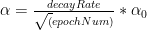
 is the learning rate. Also
  is the loss which is back propagated to the previous layers. You can see the detailed derivation of back propagation in my post


 Checkout my book ‘Deep Learning from first principles: Second Edition – In vectorized Python, R and Octave’. My book starts with the implementation of a simple 2-layer Neural Network and works its way to a generic L-Layer Deep Learning Network, with all the bells and whistles. The derivations have been discussed in detail. The code has been extensively commented and included in its entirety in the Appendix sections. My book is available on Amazon as
 then we we can represent the exponentially average value at time ‘t’ as a sequence of the the previous value
  and
and  as shown below
 represent the average of the data set over
  By choosing different values of
  , we can average over a larger or smaller number of the data points.


 , which is an exponentially decaying function.


 where
where and
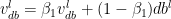
and  are the momentum terms which are exponentially weighted with the corresponding gradients ‘dW’ and ‘db’ at the corresponding layer ‘l’ The code snippet for Stochastic Gradient Descent with momentum in R is shown below


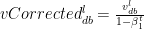
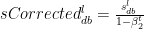
 and
and  are the RMSProp terms which are exponentially weighted with the corresponding gradients ‘dW’ and ‘db’ at the corresponding layer ‘l’