‘Would you tell me, please, which way I ought to go from here?’ ‘That depends a good deal on where you want to get to,’ said the Cat. ‘I don’t much care where—’ said Alice. ‘Then it doesn’t matter which way you go,’ said the Cat. ‘—so long as I get somewhere,’ Alice added as an explanation. ‘Oh, you’re sure to do that,’ said the Cat, ‘if you only walk long enough.’
Alice in Wonderland, Lewis Caroll, 1864
About three years ago, I implemented a T20 Match Win Probability model, using Deep Learning with batsman and bowler embeddings to compute the the ball-by-ball probability of winning by the competing teams as the match progresses (see GooglyPlusPlus: Win Probability using Deep Learning and player embeddings.). Ball-by-ball match data is available for different T20 leagues in Cricsheet. This Deep Learning algorithm was originally written in TensorFlow and Keras at that time (Win Probabilty Computation – TensorflowKeras). I had got a training and validation accuracy of around 0.8876 (this is very similar to Win Probability model in baseball, NFL etc.)
I recently, revisited this code and asked Sonnet 4.6 to convert the TensorFlow-Keras DL algorithm into PyTorch, (more compact and probably more efficient), which it promptly did, without breaking a sweat. However, even after converting to Pytorch, the validation accuracy still remained ~ 0.8959 (see notebook Match Win Probability Computation – Pytorch). The T20 Win Probability Model was trained on 2.14 million rows of T20 data taken from 9 different T20 leagues across the globe. The ball-by-ball match data is available in Cricsheet as yaml files which have been pre-processed suitably.
I was wondering whether it was possible to use Karpathy’s auto-research to optimise this DL algorithm Providentially, I came across EPOCH: An agentic protocol for multi-round system optimisation by Liu, Li, and Srikanth (2026), which was a paper that was published by my colleagues at Prorata.ai. EPOCH, enables system fine-tuning, optimisations of model, code, and rule-based components. Since, this was exactly what I wanted, I decided to give EPOCH a try. The result was quite impressive!!!
The setup and installation was pretty straightforward. I then started EPOCH by typing in /epoch in Claude Code. Initially, I was just given a set of questions. I set the goal of 0.95 as the target validation accuracy for the agentic protocol.
Incidentally, earlier, I did try a couple of things to improve the performance of the DL algorithm by playing around with the hyper-parameters, including brute-force Gridsearch, but none of it seemed to help. I think I hit a plateau around 0.8876.
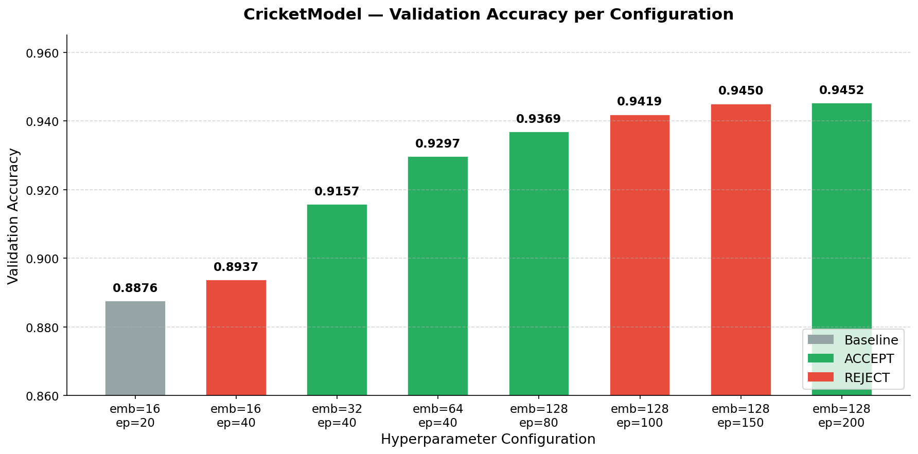
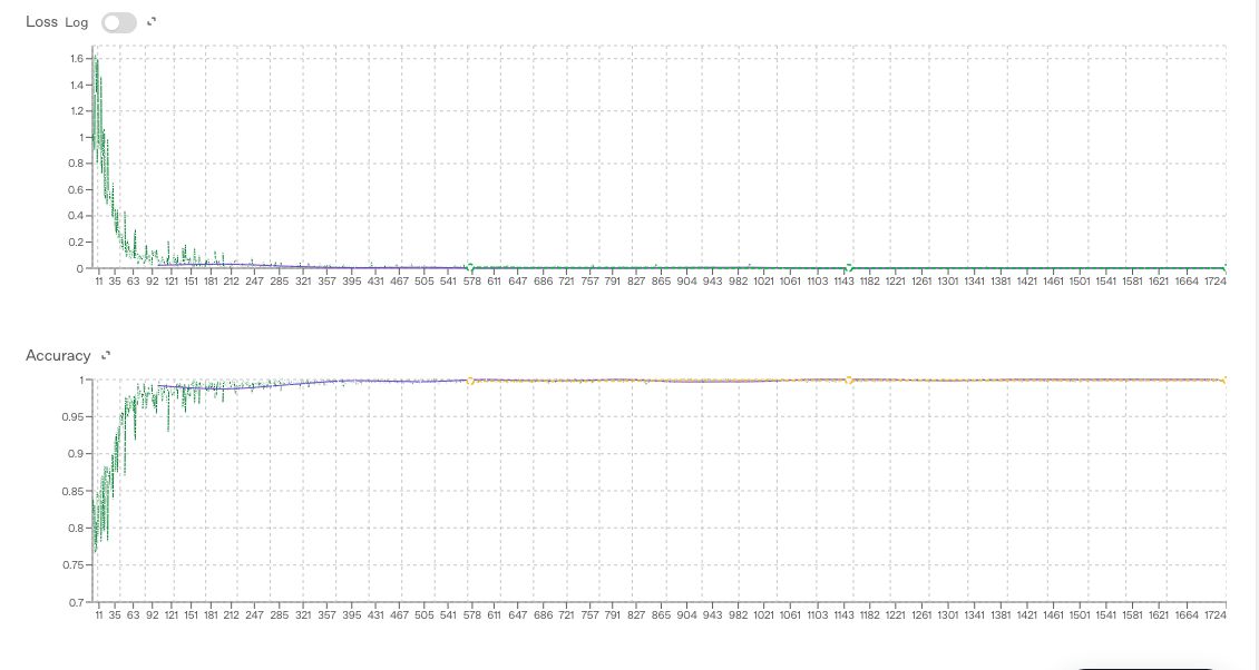
EPOCH, created an initial scaffolding and baseline metrics. It then ran multiple experiments to optimise the validation accuracy which started to inch towards 0.95. Here is a summary of the experiments of EPOCH and the outcomes. EPOCH and Claude Code stored the baseline metrics and results of each experiment in github repo claude_wpa
a) Hyperparameter tuning vsValidation accuracy improvement
Included below are the hyperparameter changes and the corresponding validation accuracy improvement in each round
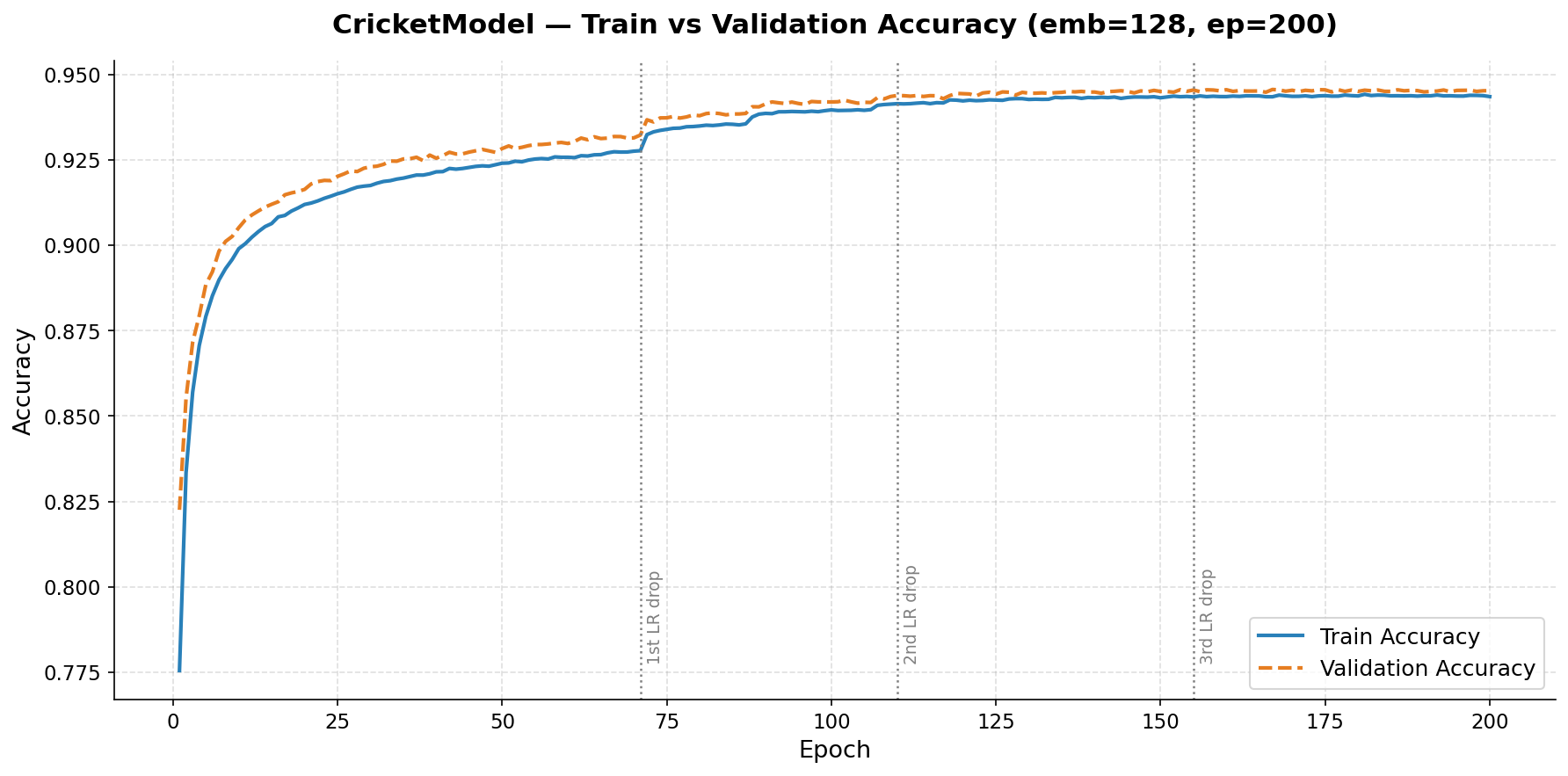
b) Train vs Validation Accuracy improvement in final round
EPOCH Optimization — Experiment Log
#
Change Made
Val Acc
Delta
Verdict
Remarks
1
Baseline: emb=16, ep=20, lr=0.01
0.8876
—
Baseline
Starting point. 16-dim embeddings for 7,785 batsmen + 5,742 bowlers is severely under-capacity.
2
epochs: 20 → 40 (emb=16)
0.8937
+0.0061
❌ REJECT
More epochs alone not enough — embedding bottleneck is the real constraint.
3
emb: 16 → 32, epochs=40
0.9157
+0.0281
✅ ACCEPT
Biggest single jump (+2.81%). Doubling embedding capacity gave the model enough room to represent player identities.
4
emb: 32 → 64, epochs=40
0.9297
+0.0140
✅ ACCEPT
Scaling embedding further yielded another solid gain. Diminishing returns beginning to show.
5
emb: 64 → 128, epochs=80, lr=0.01
0.9369
+0.0072
✅ ACCEPT
Good gain. LR scheduler fired at ep76 with only 4 epochs left — couldn’t fully exploit the reduction.
6
epochs: 80 → 100 (emb=128)
0.9419
+0.0050
❌ REJECT
2nd LR drop just starting at ep95–100 when training ended. Model plateaued at 0.9419.
7
epochs: 100 → 150 (emb=128)
0.9450
+0.0081
❌ REJECT
Progress, but just below the min_delta threshold. 3rd LR drop just beginning.
8
epochs: 150 → 200 (emb=128)
0.9452
+0.0083
✅ ACCEPT
3rd LR scheduler drop fully exploited. Well-regularized (train_eval_gap = −0.0017). Final model.
Key Findings
Finding
Detail
Embedding dim was the biggest lever
Going 16→32→64→128 drove most of the accuracy gain (+4.93% combined)
LR scheduler is crucial but fires late
ReduceLROnPlateau (patience=3, factor=0.5) fires at ~ep71, ~ep110, ~ep155 — each firing gives ~+0.005
Epochs must be long enough post-firing
Each LR drop needs ~40–50 epochs to propagate — that’s why ep=200 was needed
No overfitting throughout
train_eval_gap was always small and negative (−0.0017 to −0.0061), meaning BatchNorm+Dropout regularized well
lr=0.001 from random init causes regression
Tried lower LR early on — model under-converged. lr=0.01 with scheduler is the right combination
Total improvement: 0.8876 → 0.9452 (+6.76%) across 8 experiments.
The final trained T20 Win Probability model had a validation accuracy of 0.9452 at which point I stoppd further experiments. This model was downloaded with all the necessary metadata which included the trained weights, the architecture config, and the standard scaler, which needs to be applied on any new data on which the model is actually applied. The trained T20 Win Probability DL Model was applied the three T20 matches in the latest ICC T20 World Cup held this year from Feb 07,206 to Mar 8, 2026.
The ball-by-ball Win probability for each team in the T20 match is computed in the charts below. There will be two charts for each of the matches.
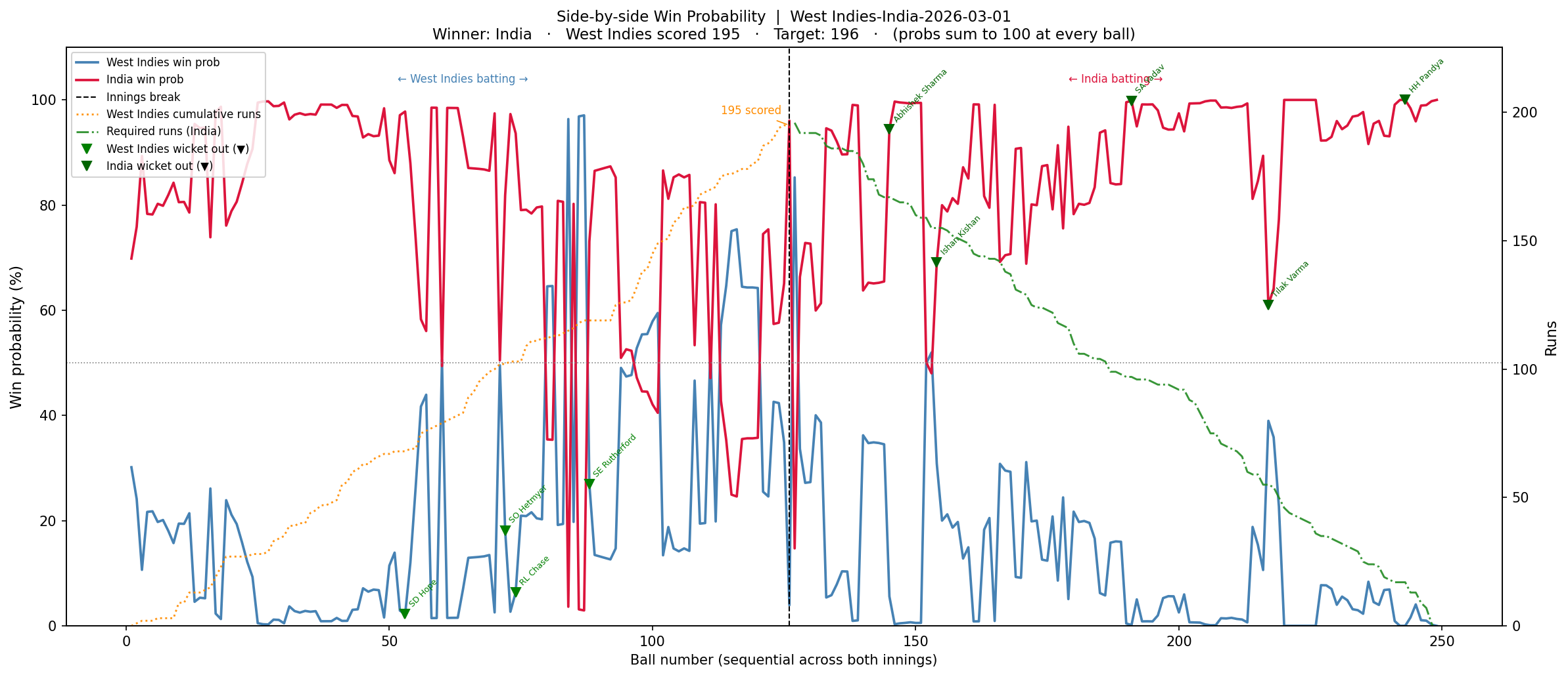
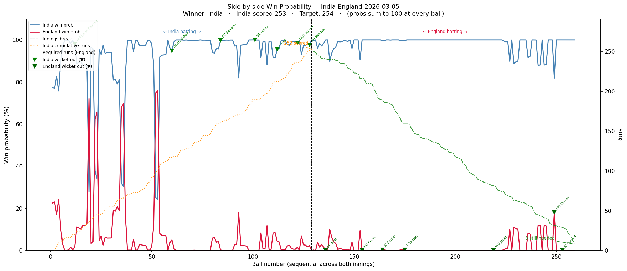
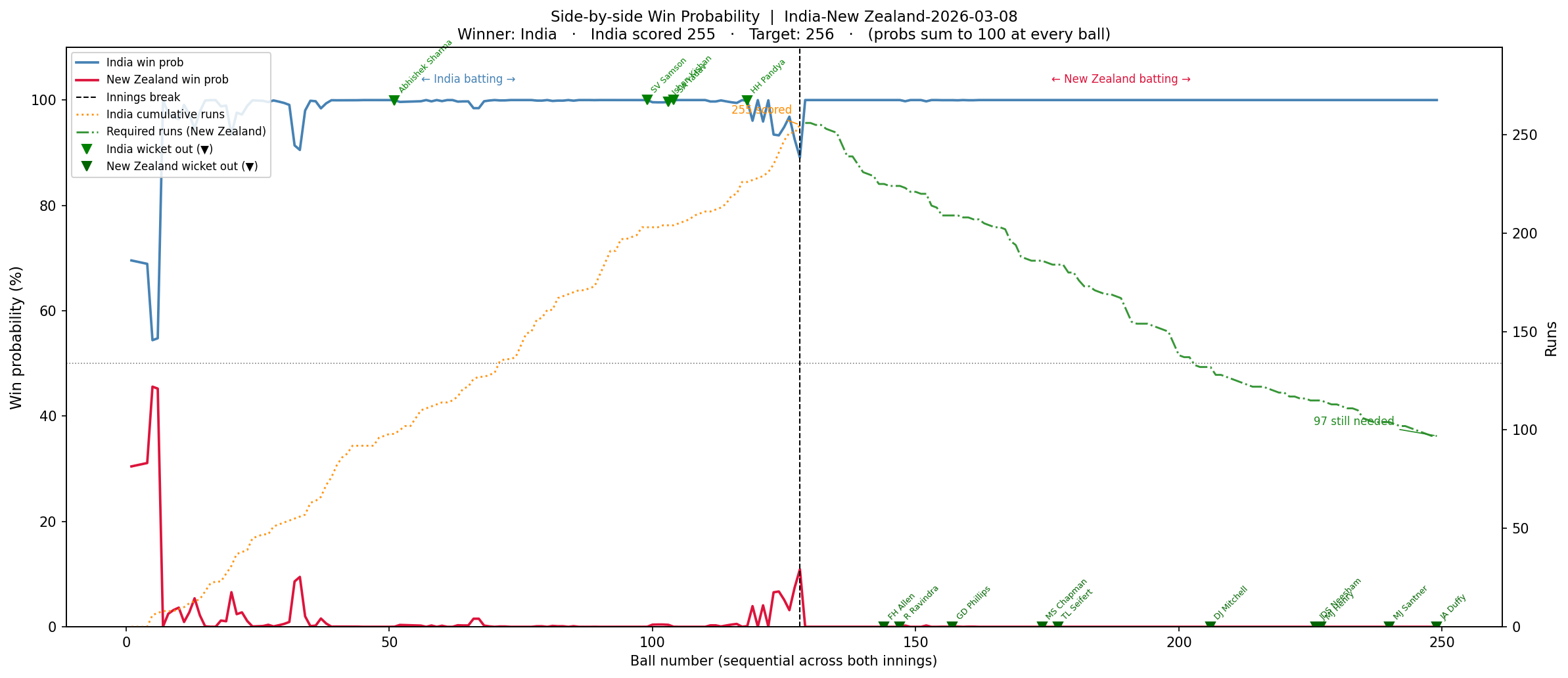
a) Win Probability- Side-by-side chart : The first chart is a side-by-side Win Probability Analysis where the win probability of each team will be computed using the DL model on a ball-by-ball basis. The win probability of the other team is just 100 minus the win probability of the first team.
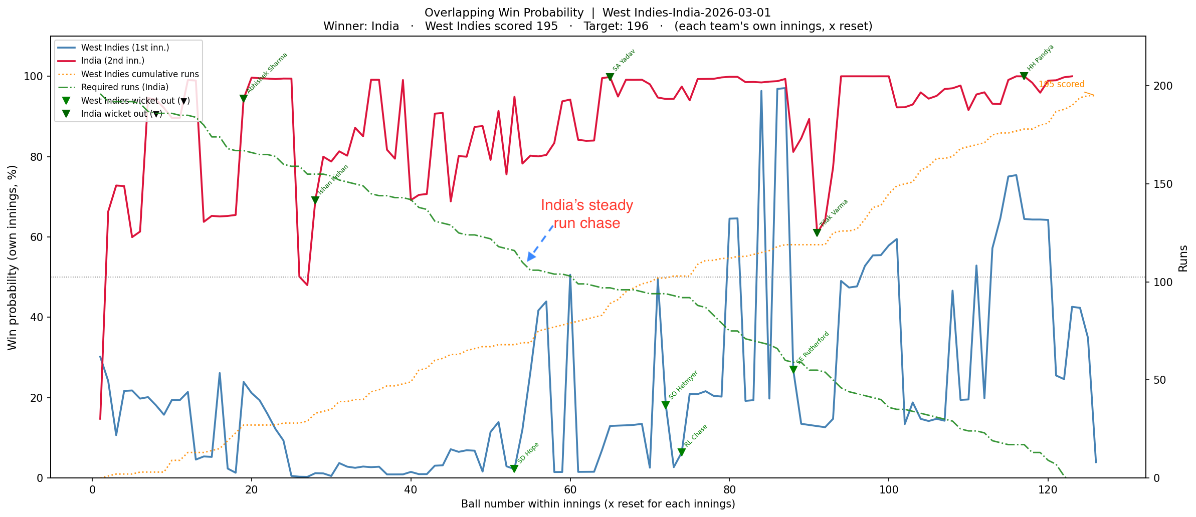
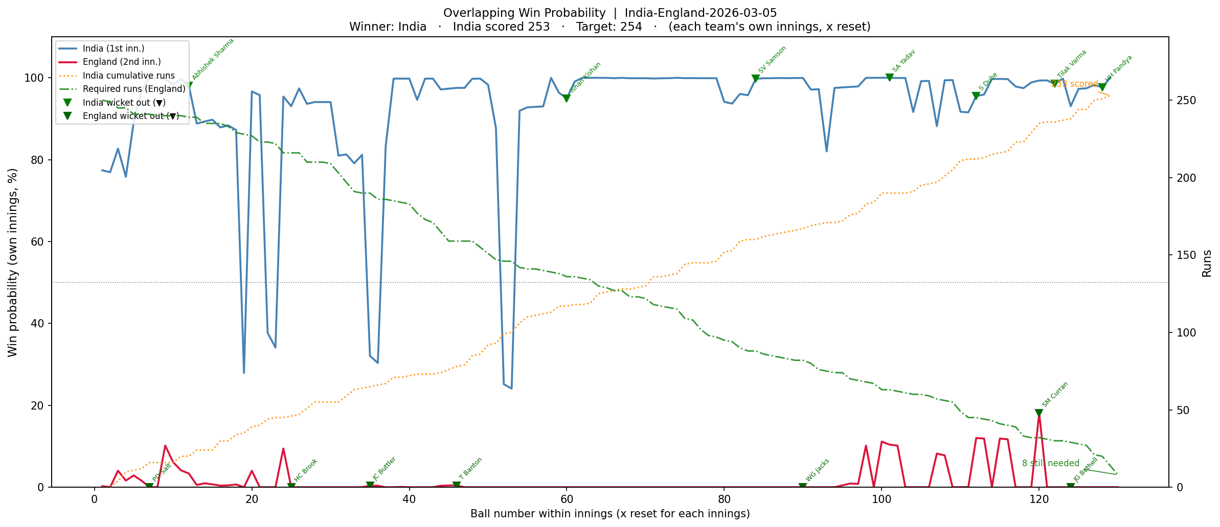
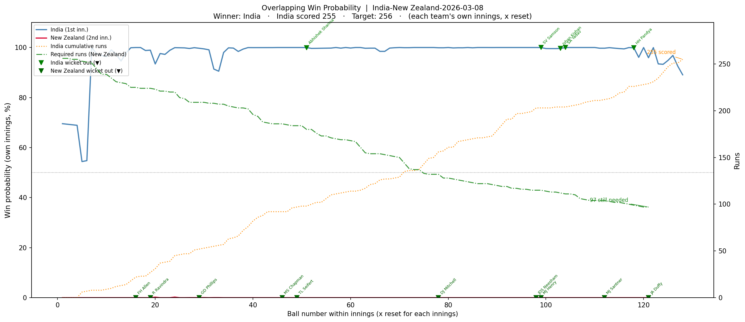
b) Win Probability – Overlapping chart : This chart will be computed using the Deep Learning model for each team independently on a ball-by-ball basis, and then both the probabilities will be super-imposed on one another so that we can see how the probability changed and whether the second team, which had to chase a total, actually was able to do so. If it could, then the win probability would actually exceed the the first team with Win Probability
I will be taking the final three matches of this ICC World Cup in 2026 namely to use the Win Proability Model against
1) West Indies vs India – Quarter Finals – Winner – India (1 Mar 2026)
In this this match, Sanju Samson stood like a rock and played a well-paced innings and chased the target comfortably scoring 97 runs not out.
a) Side-by-side chart
b) Overlapping chart
2) India vs England – Semi Finals – Winner- India (5 Mar 2026)
India set a sizable target of 253 with good contributions from Sanju Samsom, Shivam Dube and Ishan Kishan
a) Side-by-side chart
b) Overlapping chart
3) India vs New Zealand – Finals – Winner – India (8 Mar 2026)
Put into bat first, India put up a mammoth total of 255 with contributions from Sanju Samson, Abhishek Sharma, Ishan Kishan, and Shivam Dube. New Zealand lost wickets regularly and could not keep up with the required run rate, which kept climbing ever so high, so it was never in contention
a) Side-by-side chart
b) Overlapping chart
Conclusion
It was quite interesting to see agentic protocol EPOCH work. Things have really changed these days, with the agents automatically making judgement calls on what would be hyper-parameter changes would result in better performance. I remember I had used Grid Search to optimise the DeepLearning algorithm, but it didn’t help much.
Tomorrow and tomorrow and tomorrow Creeps in this petty pace from day to day To the last syllable of recorded time, And all our yesterdays have lighted fools The way to dusty death. Out, out, brief candle!
Life’s but a walking shadow, a poor player That struts and frets his hour upon the stage And then is heard no more. It is a tale Told by an idiot, full of sound and fury, Signifying nothing.
Macbeth, Act V, Scene Vby William Shakespeare
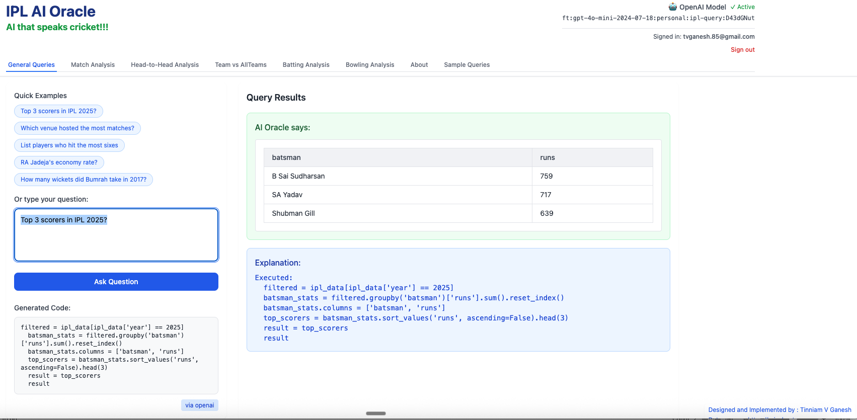
The IPL 2026 carnival is just around the corner, and my enhanced IPL app “IPL AI Oracle” is just in time for IPL fans. The current version of IPL AI Oracle, refines my earlier implementation to be more accurate and to handle a wider range of natural language queries related to IPL. My previous post “Introducing IPL AI Oracle: AI that speaks cricket!!! discusses an implementation which had 4 tabs
General queries
Match Analysis
Head-to-head
Team vs All Teams
The data for this app comes from Cricsheet. The data consists of ball-by-ball data for all IPL matches since 2006 in yaml format. This data was then pre-processed into a suitable format for use by the tabs both for the analytics and the natural language query functionality
The tabs provide analytics of IPL matches, head-to-head and team vs All Teams. Each of the 4 tabs allow for user query in natural language based on the tab general queries, queries on IPL matches, queries on head-to-head performance between 2 teams and natural language queries between a team versus All Teams.
For details about the implementation, please see the post “Introducing IPL AI Oracle: AI that speaks cricket!!! The IPL analytics are based on my Python package ‘yorkpy‘. which itself is based on its earlier avatar ‘yorkr‘ in R available in CRAN. For handling the natural language queries, in my previous implementaion, I used prompt templates for each of the tabs which would construct an appropriate prompt to gpt-4.1-nano LLM. Ths earlier implementation with prompt templates worked fine for a reasonable number of user queries. However, for each user query the prompt constructed was quite large and guzzled up tokens quite fast and I was running out of my subscription very early.
So, in this current implementation I finetune gpt-4o-mini-2024-07-18, one of the smaller gpt models, to keep the costs low. The prompt templates were reduced to the bare minimum. The gpt-40-mini-2024-17-18 model is then trained on hand-created individual training examples for each tab. The initial set of training examples was around 220 queries with corresponding pandas code. The split is as follows
matches: 65 rows
head_to_head: 50 rows
teamVsAllTeams: 48 rows
general_queries: 39 rows
This is the ground truth from which all other examples were created. Subsequently, I used Claude Sonnet 4.5 to augment the initial set of questions. The amplification essentially consisted of different ways of asking the same query for example
What is V Kohli’s strike rate in IPL?
Show me V Kohli’s strike rate
V Kohli’s strike rate
Display V Kohli’s strike rate etc
Can you tell me V Kohli’s Strike rate
Find V Kohli’s Strike rate
…
The augmented data set was used in finetuning. The finetuning process was done several times as I would take each finetuned model and test it manually. I would find issues. Sometimes the question pattern itself would be missing or it would generate incorrect response Fortunately Sonnet 4.5 helped me to identify patterns which were under-represented or were inconsistent with other queries with similar patterns. Additional training examples were added for complex queries which required the generation of a lot of code for e.g. the batting or bowling scorecard in matches, head_to_head or teamAllTeams
The original training examples are augmented to produce 2760 examples with 12 variations for simple patterns and 15 training examples for complex ones. The scorecard code is further boosted and the final number of training examples are 3831 training data which cannbe split into
matches: 1212 examples
head_to_head: 1032 examples
teamVsAllTeams: 1002 examples
general_queries: 585 examples
This training data is then shuffled and split into training and validation in the ratio of 3447 (90%) : 384 (10%).
The base model was gpt-4o-mini-2024-07-18 which was the smallest and most economical. The default hyper parameters were used
Epochs – 3
Batch size – 6
LR multiplier – 1.8
Seed – 3
Train loss – 0.000
Validation loss – 0.003
Full validation loss – 0.002
Try out the enhanced IPL AI Oracle – https://wizard-ai-three.vercel.app/ (When you click the above link, a page will open. Enter your email and click ‘Send magic link‘ button below. This will send a magic link to your email. Click the ‘Sign in’ button which will allow you login to the app IPL AI Oracle and start using it.)
Natural language queries
Here are some random natural language queries in different tabs
A) General queries tab
This tab deals with general on IPL queries
1) Top 3 scorers in IPL 2025?
…
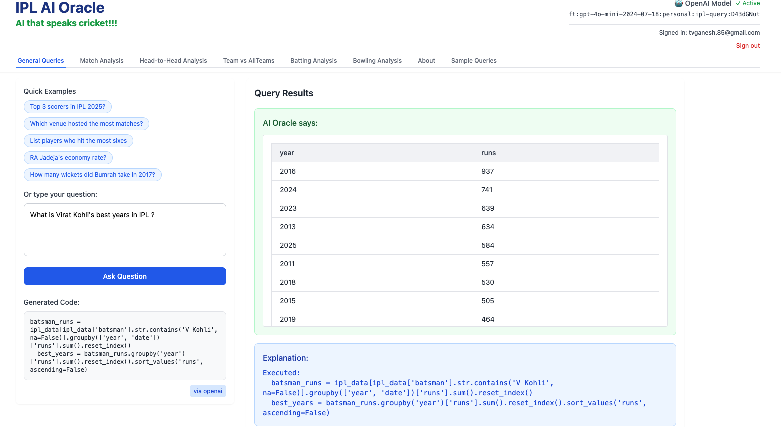
2) What is Virat Kohli’s best years in IPL?
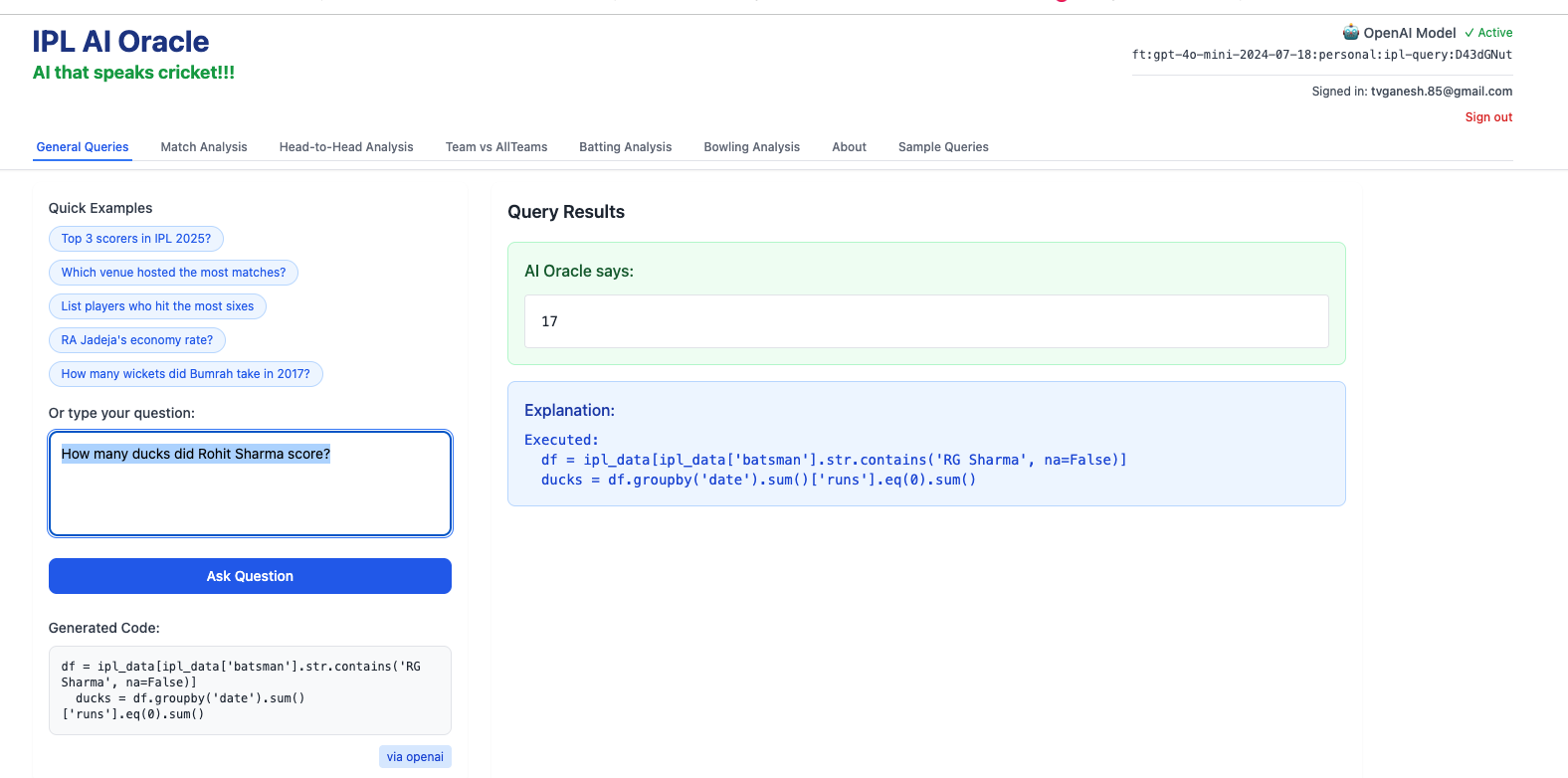
3) How many ducks did Rohit Sharma score in IPL?
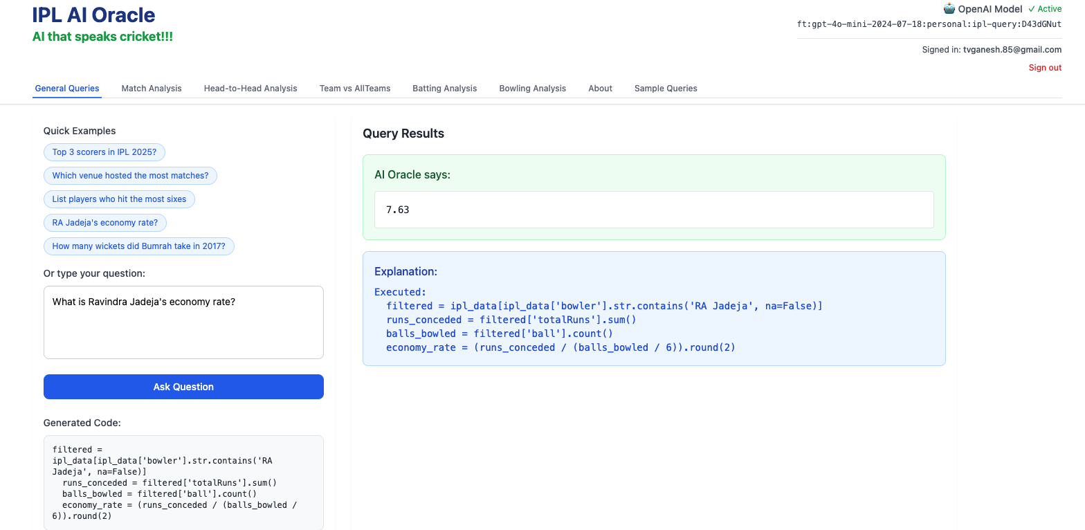
4) What is Ravindra Jadeja’s Economy rate?
B) Matches tab
This tab deals with a selected individual match
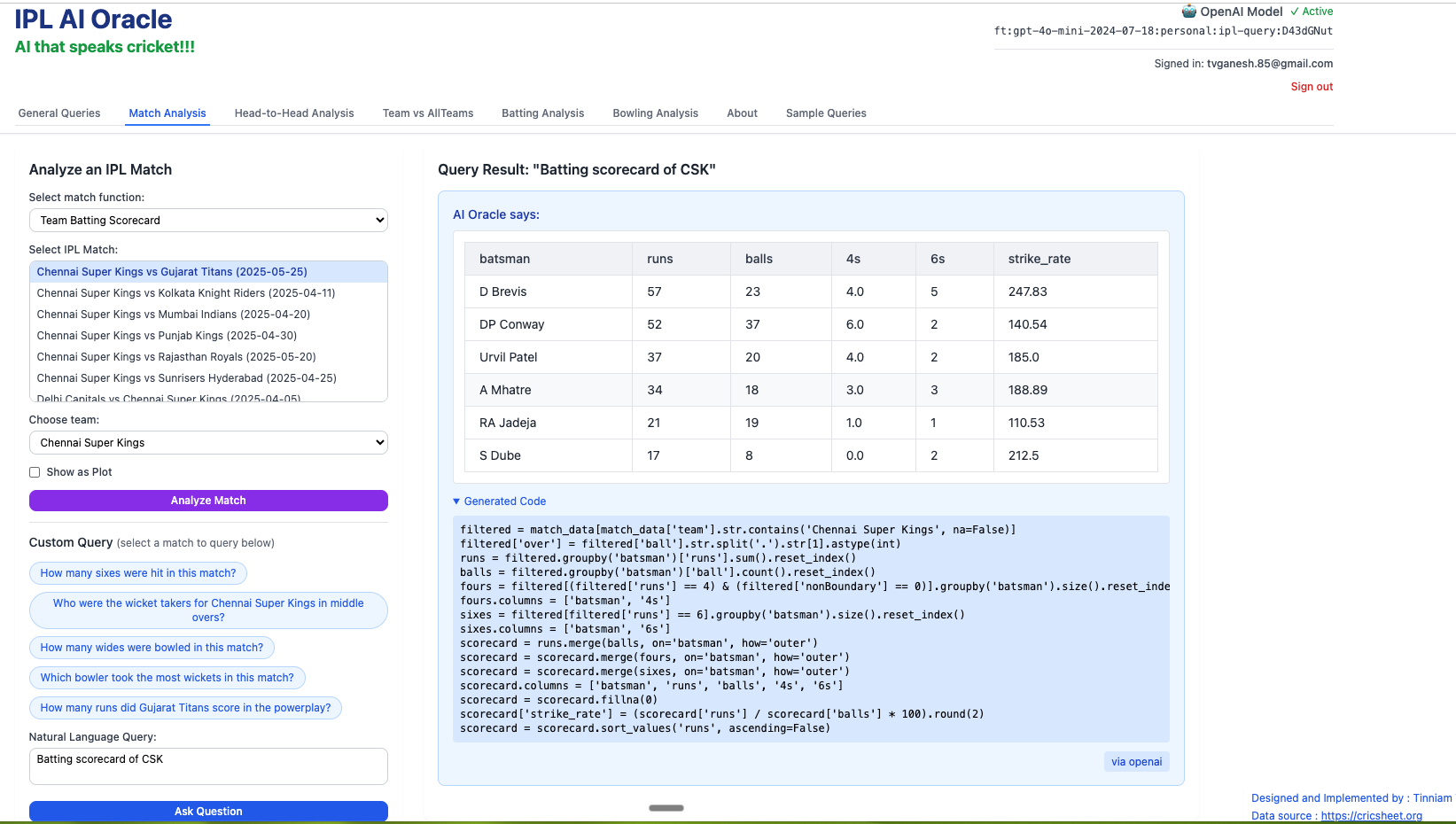
Batting scorecard of CSK
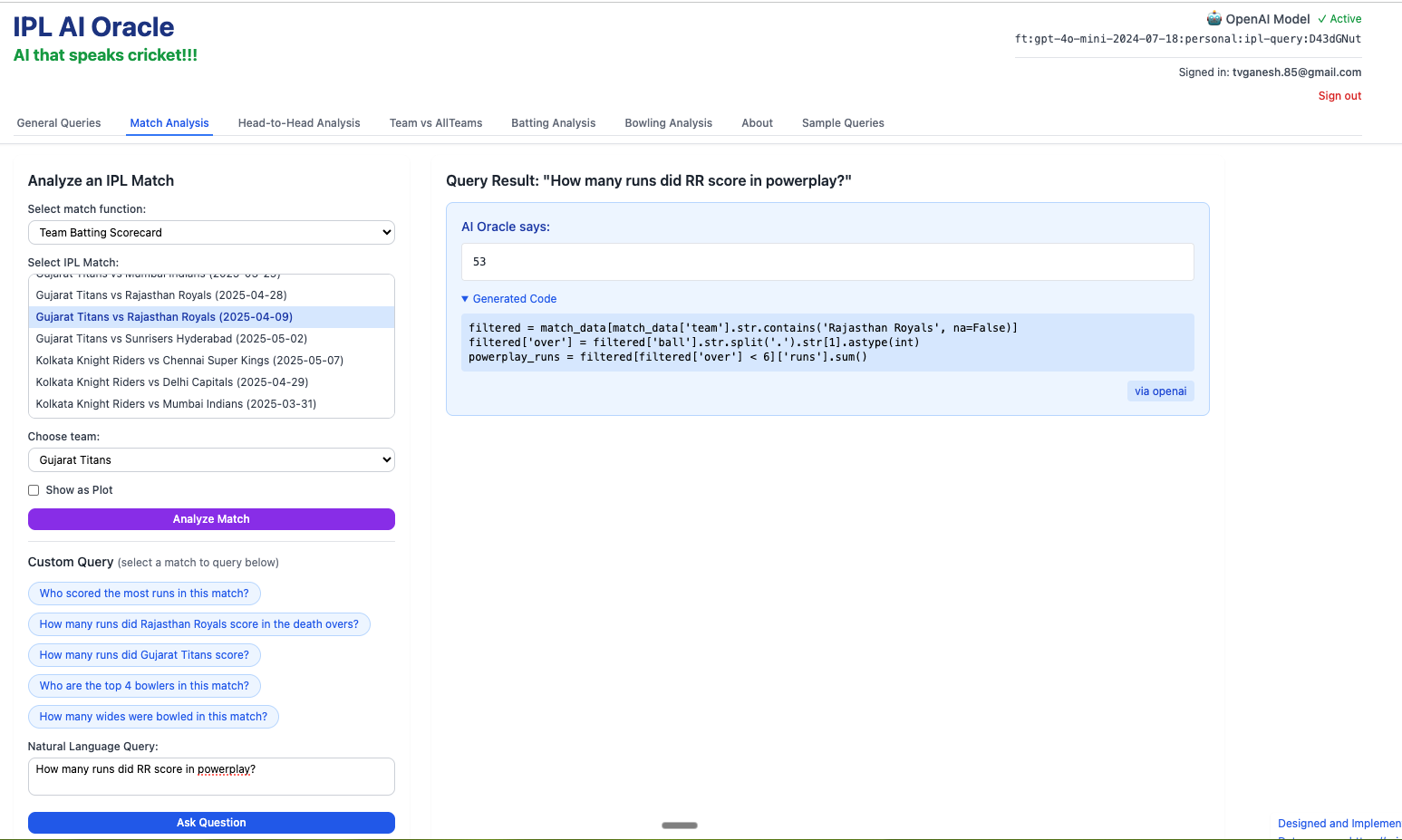
2) How many runs did RR score in powerplay?
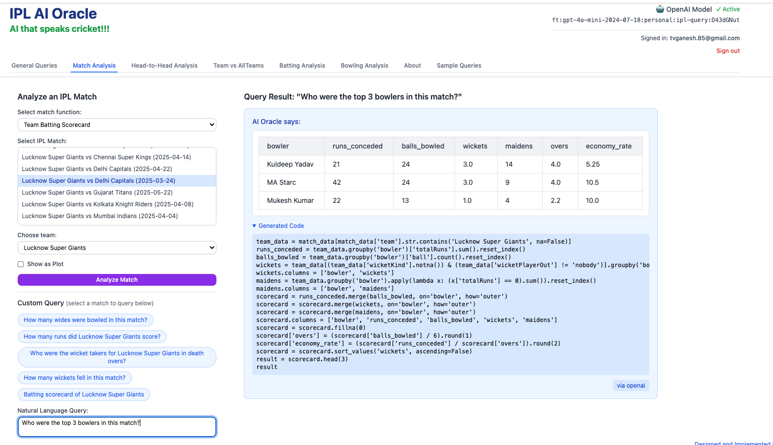
3) Who were the top 3 bowlers in this match?
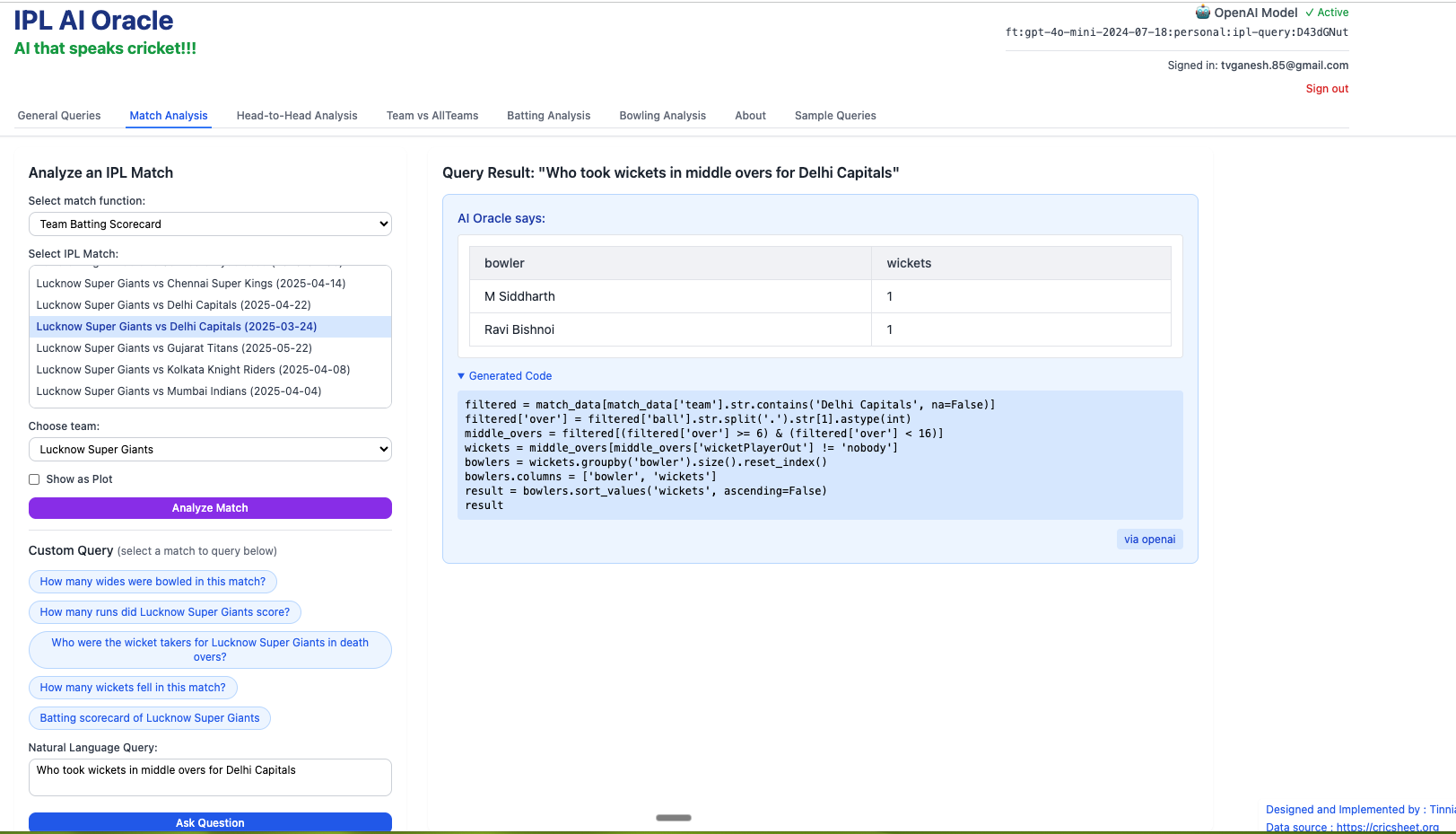
4) Who took wickets for in middle overs for Delhi Capitals?
C) Head to head tab
This tab takes into consideration all matches played between the 2 selected teams
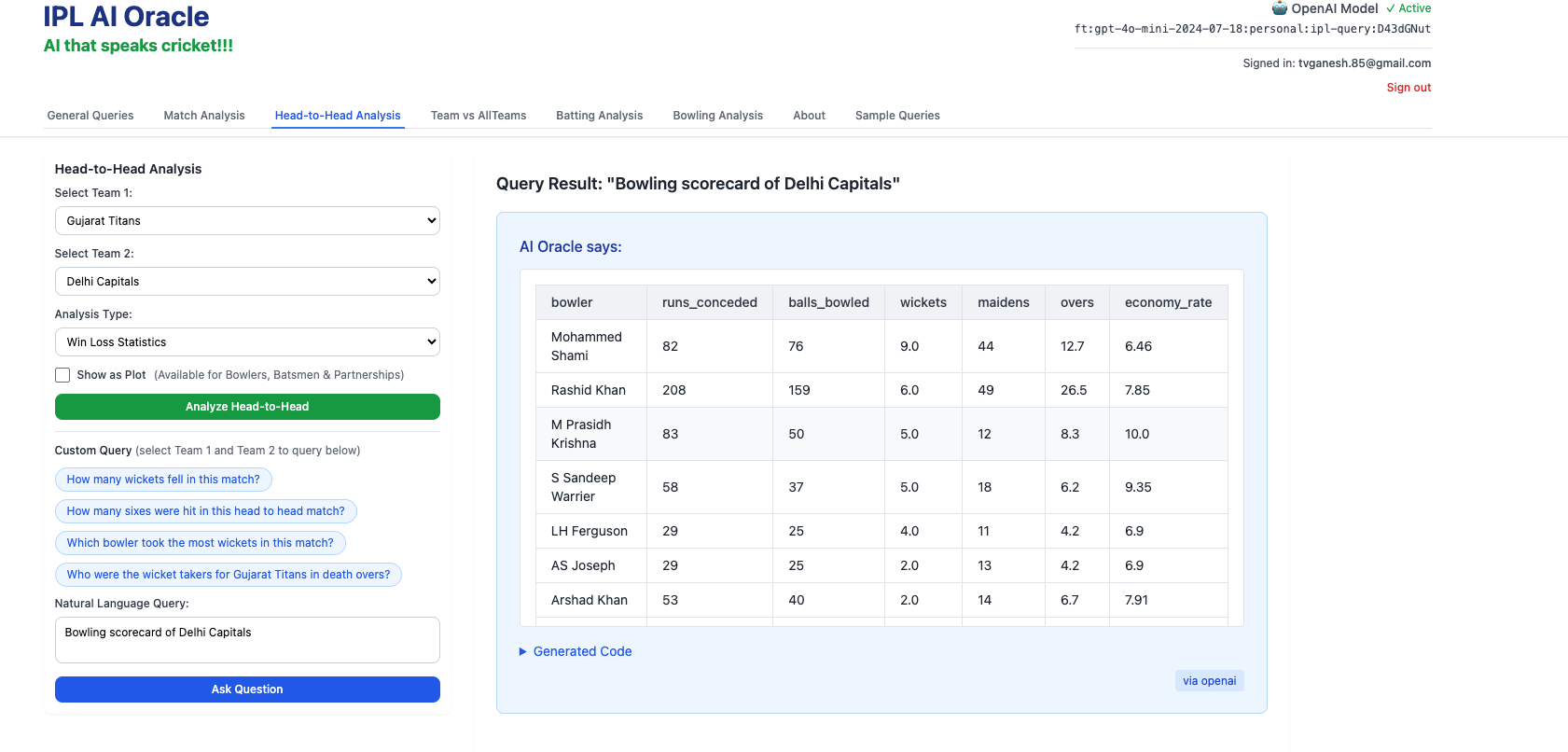
Bowling scorecard of Delhi Capitals
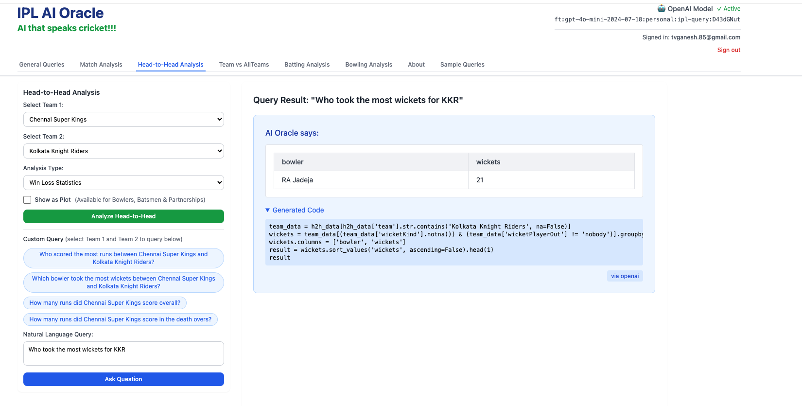
2. Who took the most wickers for KKR?
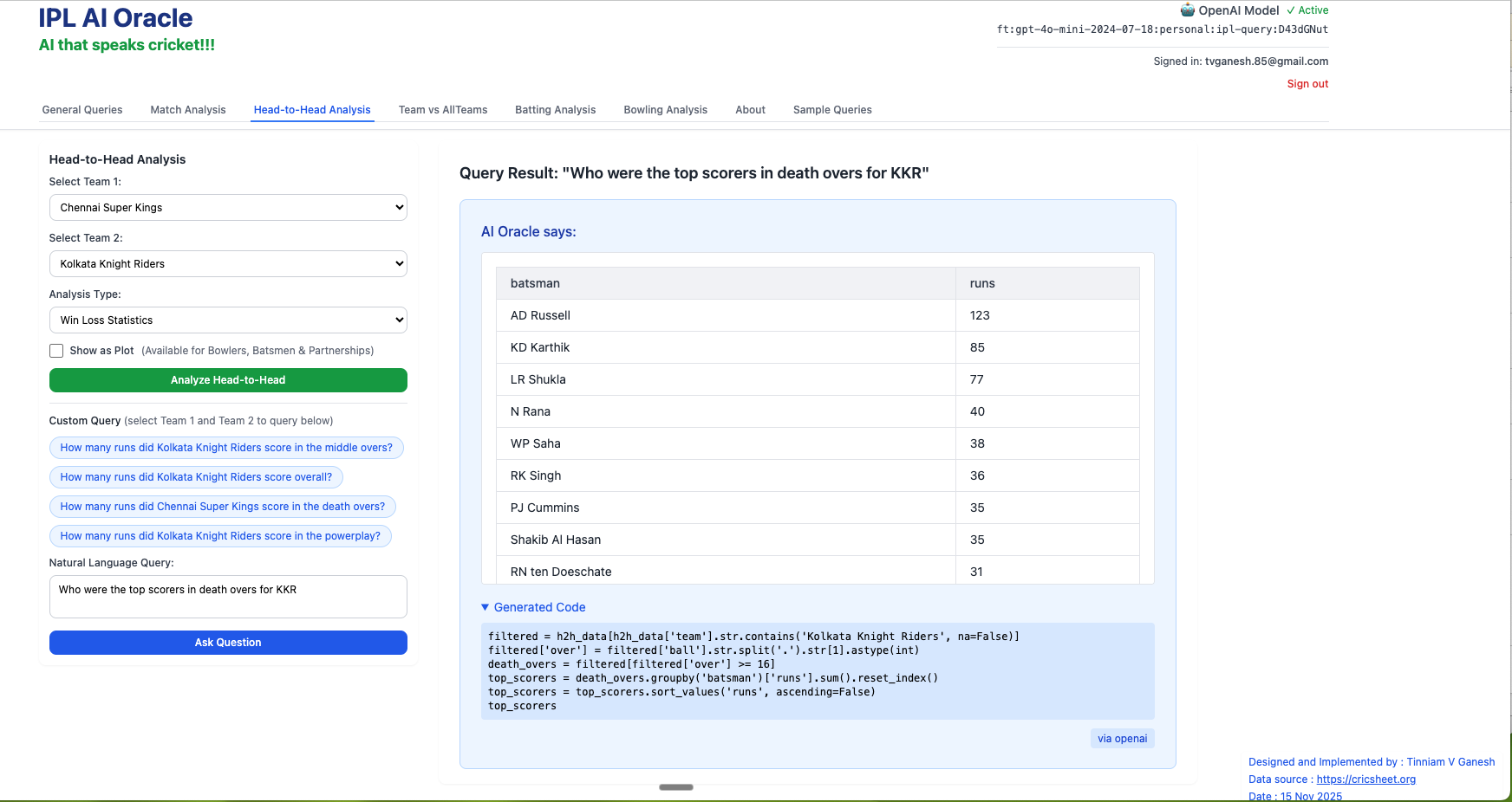
3) Who were the top scorers for KKR in death overs?
D) Team vs All Teams
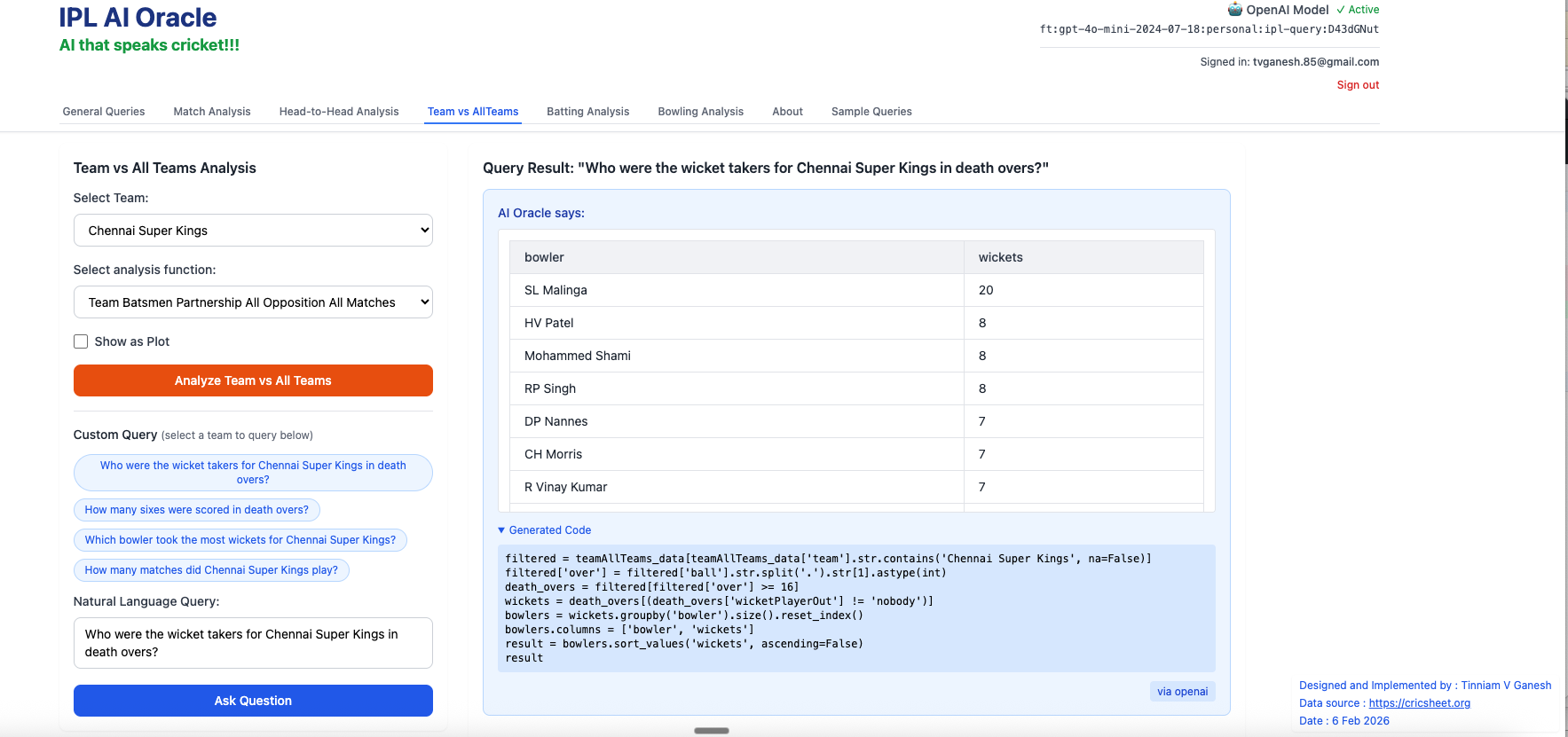
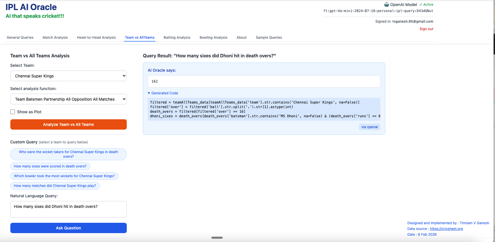
Who were most wicket takers for Chennai Super Kings in death over?
2. How many sixes did Dhoni hit in death overs?
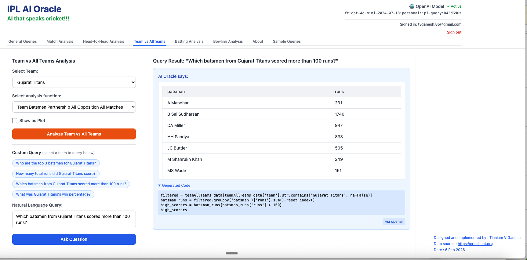
3. Which batsmen from Gujarat Titans scored more than 100 runs?
In addition I have added 2 other tabs to the earlier tabs. Now there is
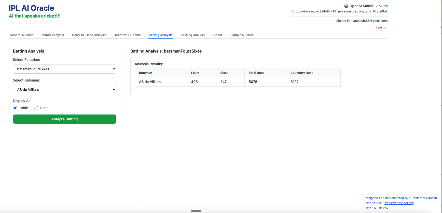
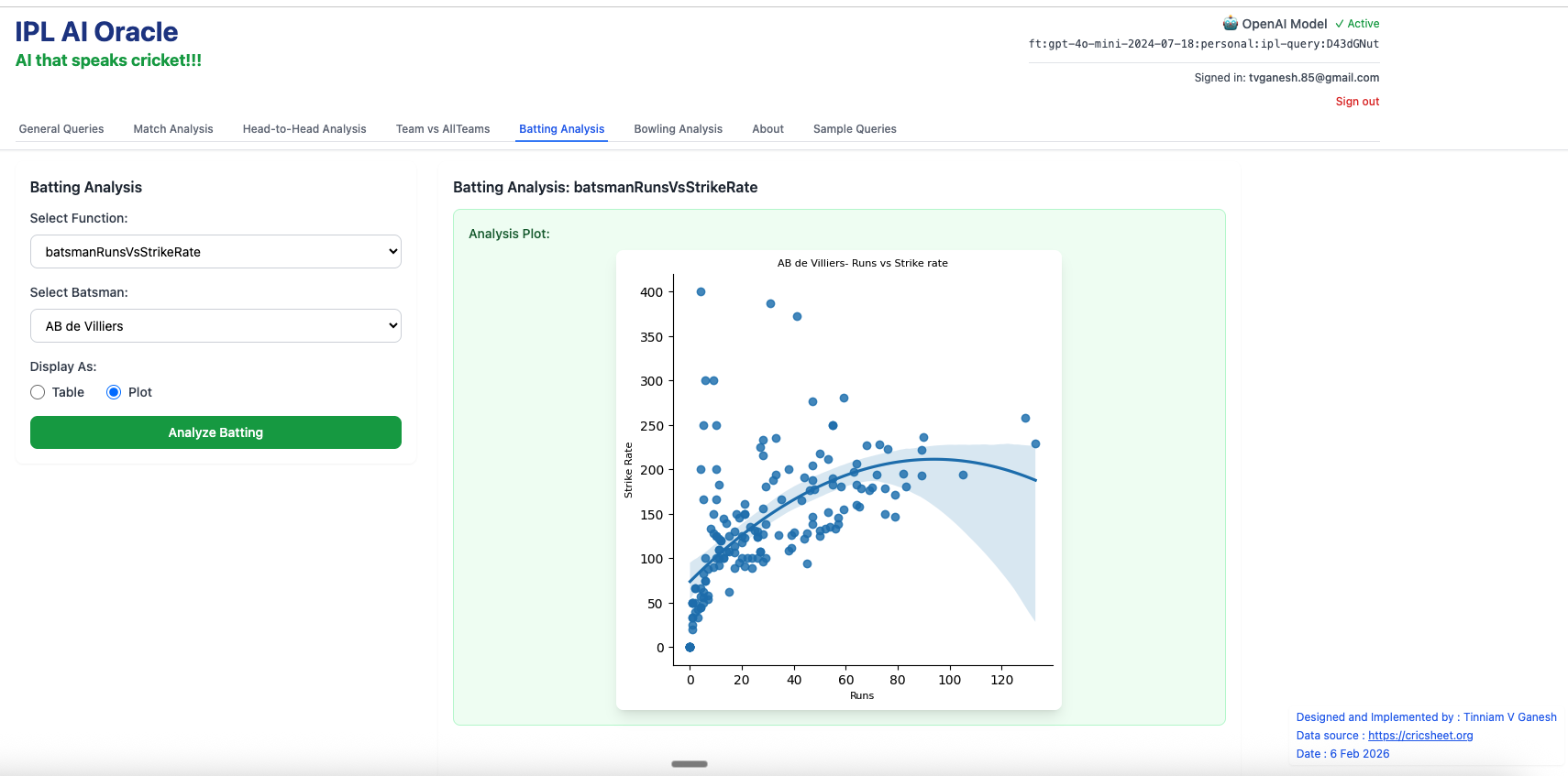
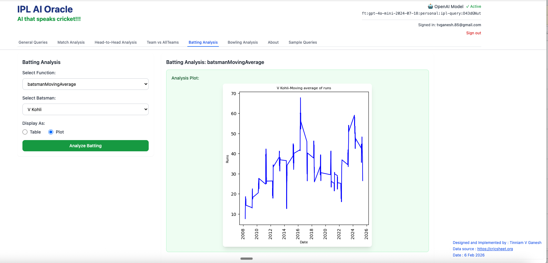
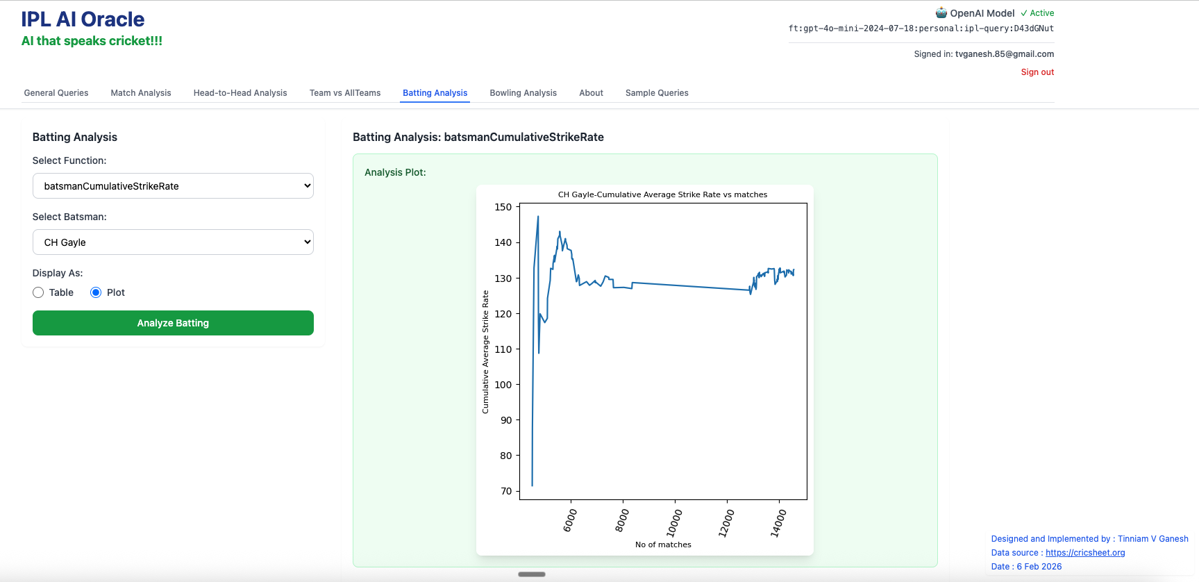
Batting Analysis tab
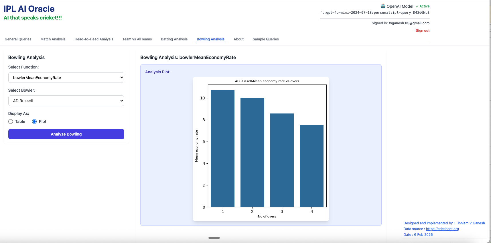
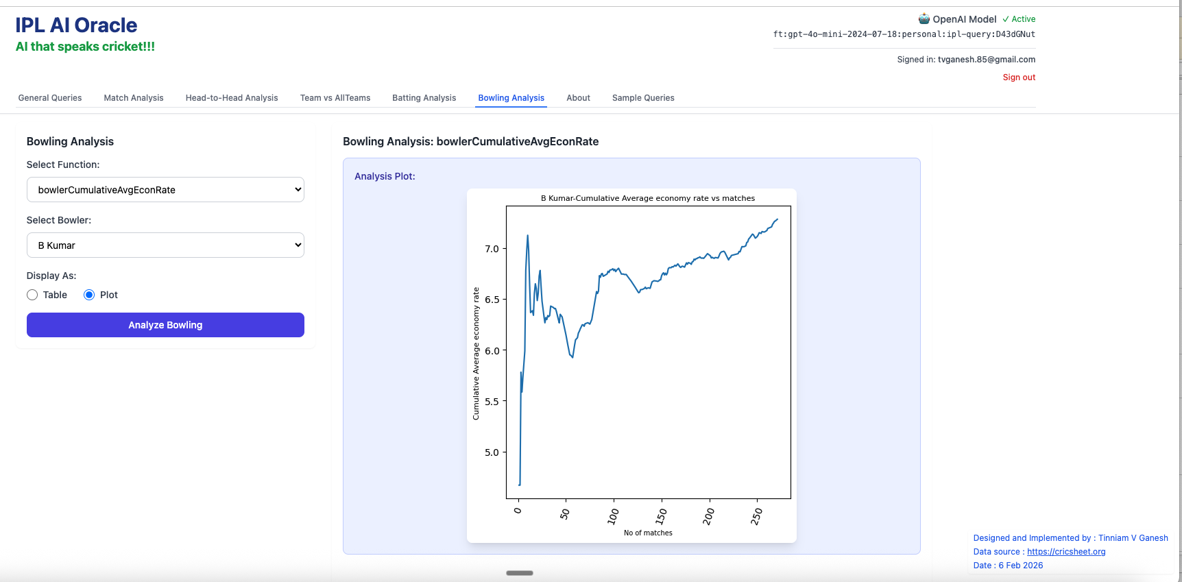
Bowling Analysis tab
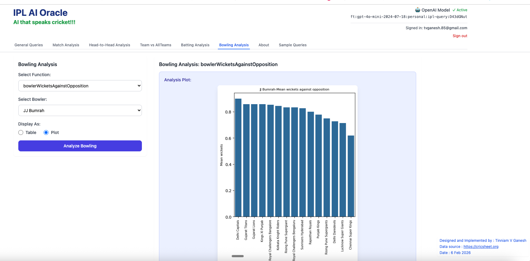
These tab provide various batting and bowling analytics for IPL players
IPL AI Oracle can make mistakes and sometimes generate erroneous code
If the answer is wrong try to rephrase the question.
Try to use the full name Rohit Sharma if possible
You can use abbreviations like ER, SR and for teams CSK, RCB, KKR etc
IPL AI Oracle is not always one shot, sometimes it is 2-shot
I will try to improve the model in future versions. For the current version I had to do some of the steps including the testing manually. I would like to experiment with Claude Code and automate the generation of training data, finetuning, testing using the finetuned model (using a test harness) and subsequently correcting/adding to the training data if needed repeating the steps again till the tests pass with a high degree of accuracy. Lets see.
What would you think if I sang out of tune? Would you stand up and walk out on me? Lend me your ears and I’ll sing you a song And I’ll try not to sing out of key
Oh, I get by with a little help from AI Mm, I get high with a little help from AI Mm, gonna try with a little help with AI
Adapted from “With A Little Help From My Friends” from the album Sgt. Pepper’s Lonely Heart Club Band, Beatles, 1967
Introduction For quite some time I have been wanting to create an application that allows user to query cricket data in plain English (Natural Language Query) and get the appropriate answer. Finally, I have been able to realise this idea with my latest application “IPL AI Oracle:AI that speaks cricket!!!“. While I have just done this for IPL, it can be done for any of the other T20 leagues namely (Intl. T20 Men’s and Women’s, BBL, PSL, NTB, CPL, WBBL etc.). The current app “IPL AI Oracle” is in Python, and is a distant cousin of my Shiny app GooglyPlusPlus written entirely in R (see IPL 2023:GooglyPlusPlus now with by AI/ML models, near real-time analytics!)
GooglyPlusPlus is much more sophisticated with detailed analytics of batsmen, bowlers, teams, matches, head-to-head, team-vs-AllTeams, batsmen and bowler ranking and analyis. GooglyPlus also includes ball-by-ball Win Probability models using Logistic Regression and Deep Learning models. While, ‘IPL AI Oracle’ lacks the ML/DL models it includes the ability to answer user queries in simple English (Natural Language Query -NLQ) and generate the pandas code for the same.
IPL AI Oracle
The IPL AI Oracle has a 2 main modules
frontend
backend
a) Frontend
The frontend is made with Next.js, Typescript and has 4 tabs
General queries
Match Analysis
Head-to-head
Team vs All Teams
The frontend includes analytics for matches, head-to-head and team-vs-allTeams options. Plots can be generated for some features and uses Plotly.js for rendering of plots
b) Backend
The backend implements FastAPI endpoints for the different analytics and natural language queries. A) The analytics in the 3 tabs namely match analysis, head-to-head and team vs All teams are implemented using my Python package ‘yorkpy‘. Since my package yorkpy has all the cricket rules baked into it, I used the code from my package verbatim for these tabs.
B) The data for the analytics comes from Cricsheet. Cricsheet includes ball-by-ball data in yaml, for all IPL matches from the beginning of time. This data is pre-processed with R utilities of my Shiny app GooglyPlusPlus. These R functions to convert the match data into the data required format for the a) Match Analysis Tab b) Head-to-head tab and c) Team vs All Teams tab which are then subsequently converted to csv for use by my package yorkpy. My Python package is based on pandas and can process this data and display the analytics required for the tabs
C) Plotly is used for generating the plots
D) Jinja templates are used for creating the prompts for the different tabs
D) For natural language query in each tab, originally I used Ollama and tried out Mistral 7Band DeepSeek Coder 6.7B. But then I realised that it has a large footprint, if deployed, and hence settled for gpt-4.1-nano
The frontend is deployed on Vercel and the backend is dockerised and deployed on Railway. Since the clock is ticking for Vercel, Railway and GPT API, I will be closely monitoring the usage.
Give IPL AI Oracle a try. Click this link IPL AI Oracle. (When you click the link you will be asked to enter your email address, to which a magic link will be sent. Clicking the link will give access to the link. Please wait 2-3 minutes for the mail, if still not received check your spam/trash folder)
Here are some random screenshots from the different tabs
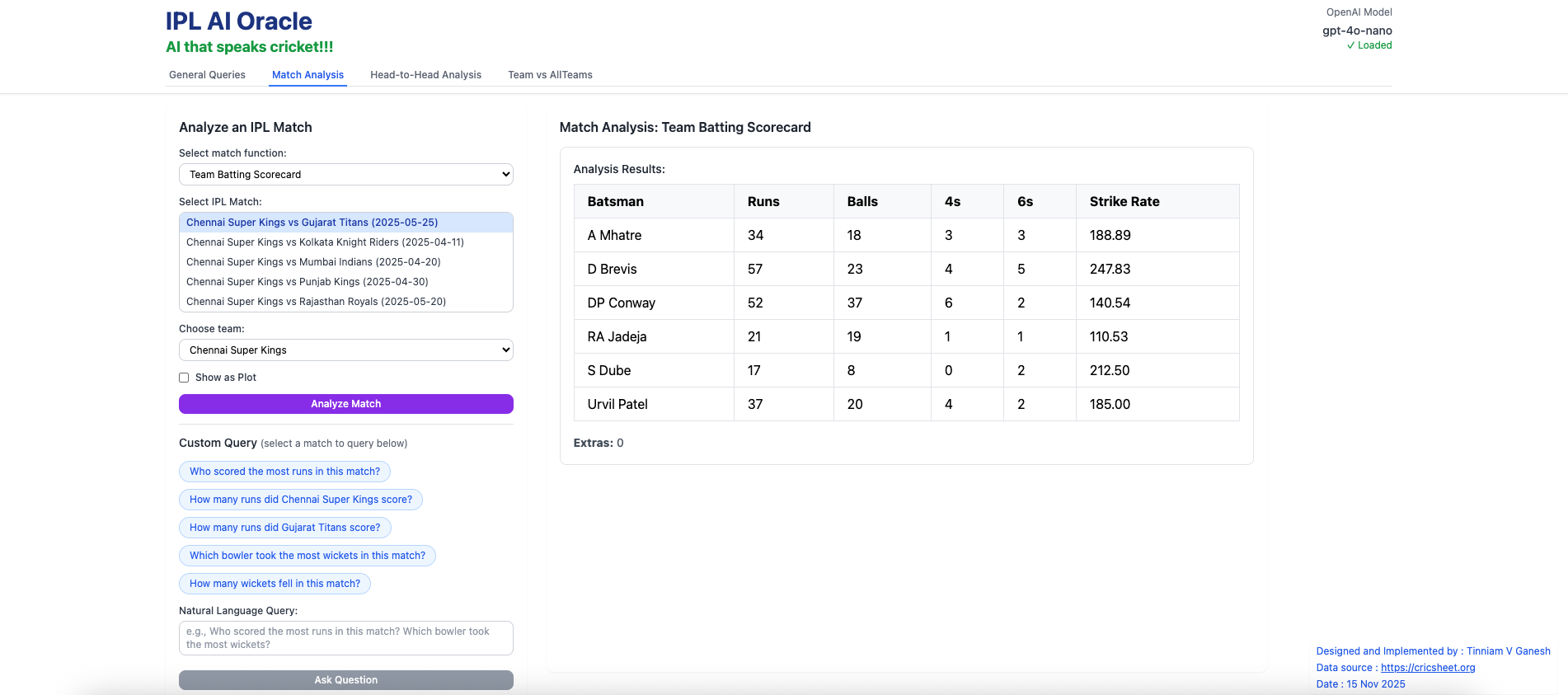
I) IPL Analytics A) Match Analysis a) Batting scorecard – Chennai Super Kings vs Gujarat Titans (2025-05-25)
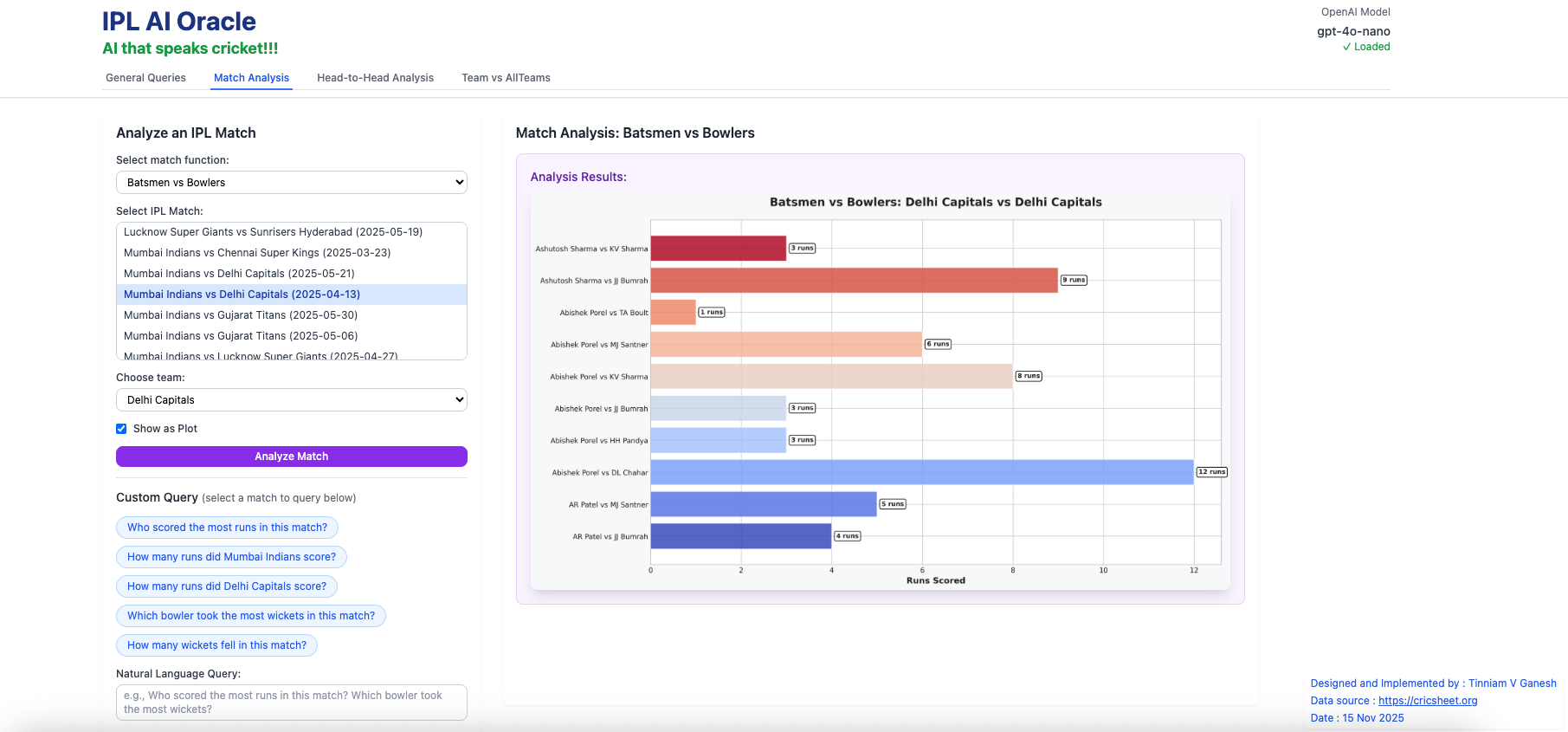
b) Batsmen vs Bowlers (Mumbai Indians vs Delhi Capitals – 2025-04-13)
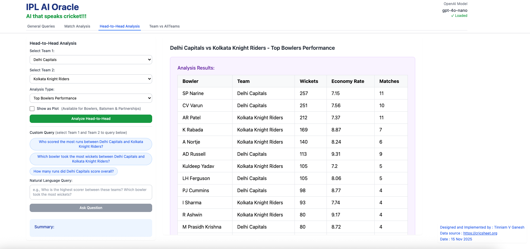
B) Head-to-head Analysis
a) Top Bowlers Performance (Delhi Capitals vs Kolkata Knight Riders – all matches) This tab takes into consideration all matches played between these 2 teams and computes analytics between these 2 teams
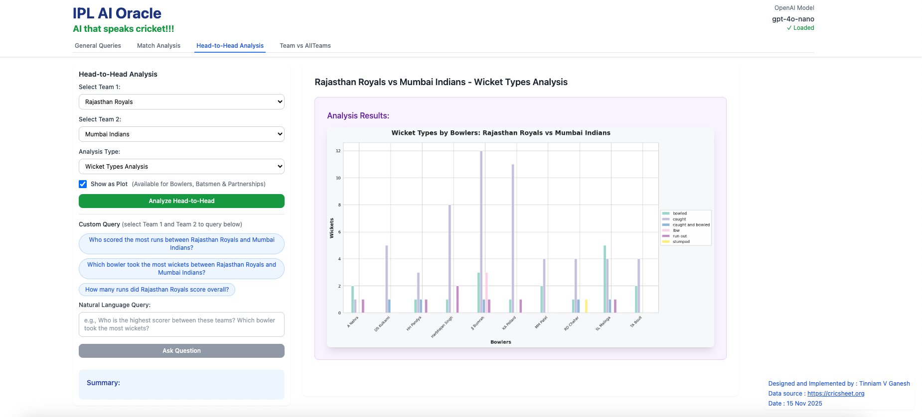
b) Wicket Types Analysis (Rajasthan Royals vs Mumbai Indians – all matches)
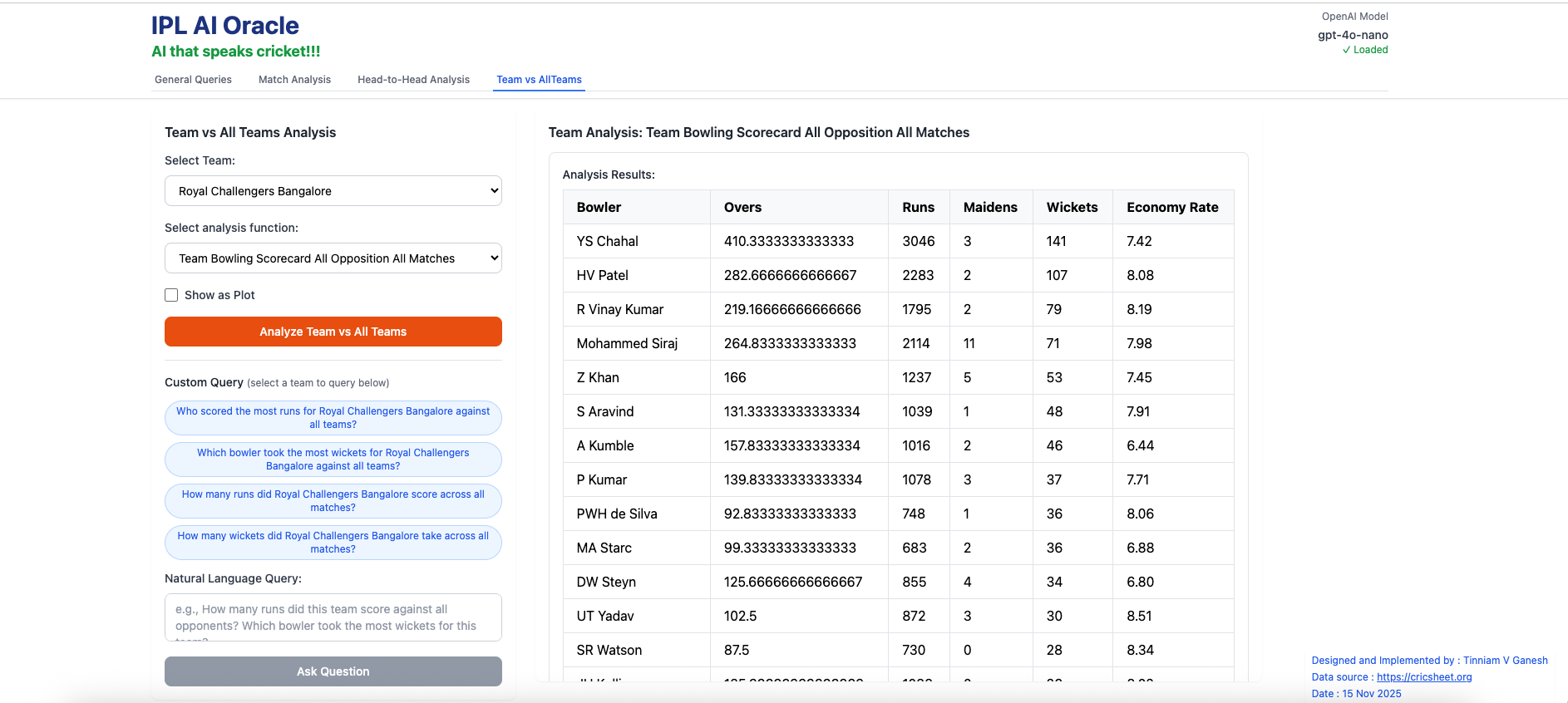
C) Team vs All Teams
a) Team Bowling Scorecard – Royal Challengers Bangalore
II) Natural Language Query (User queries)
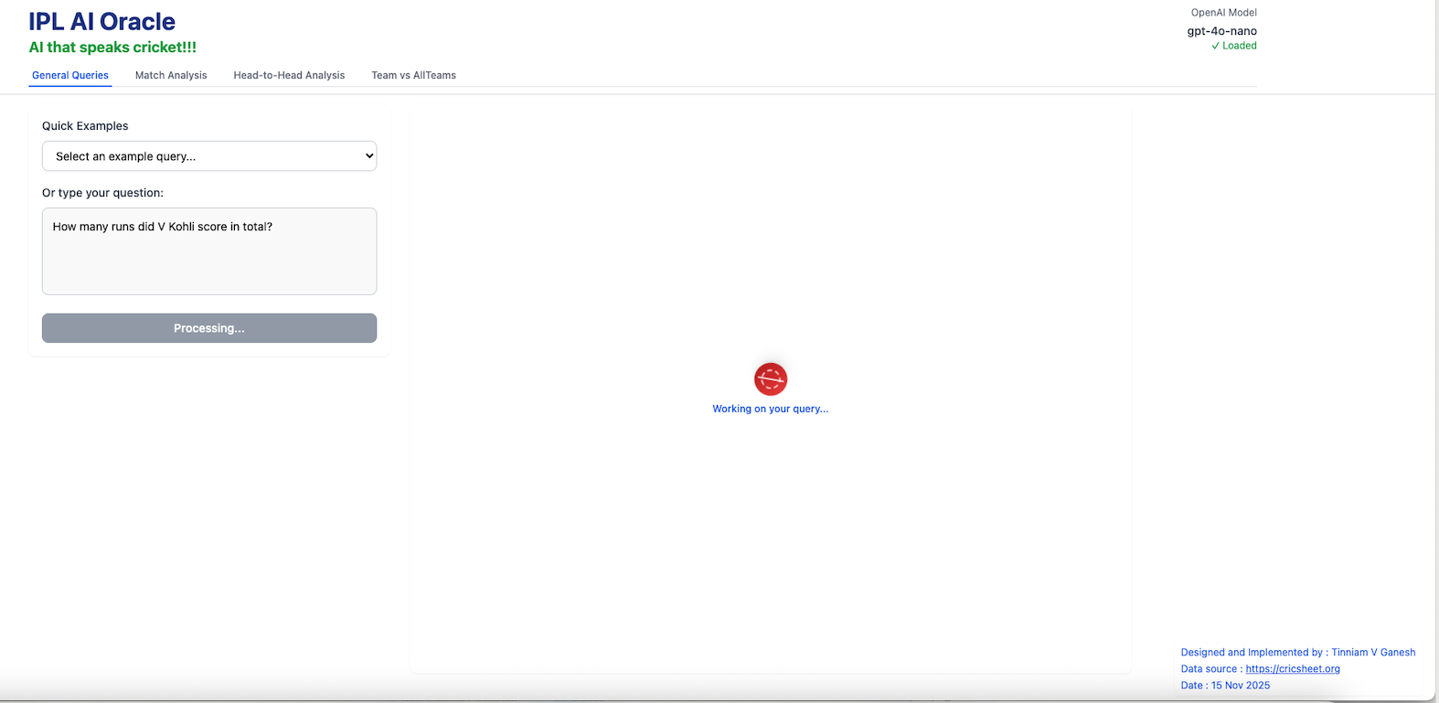
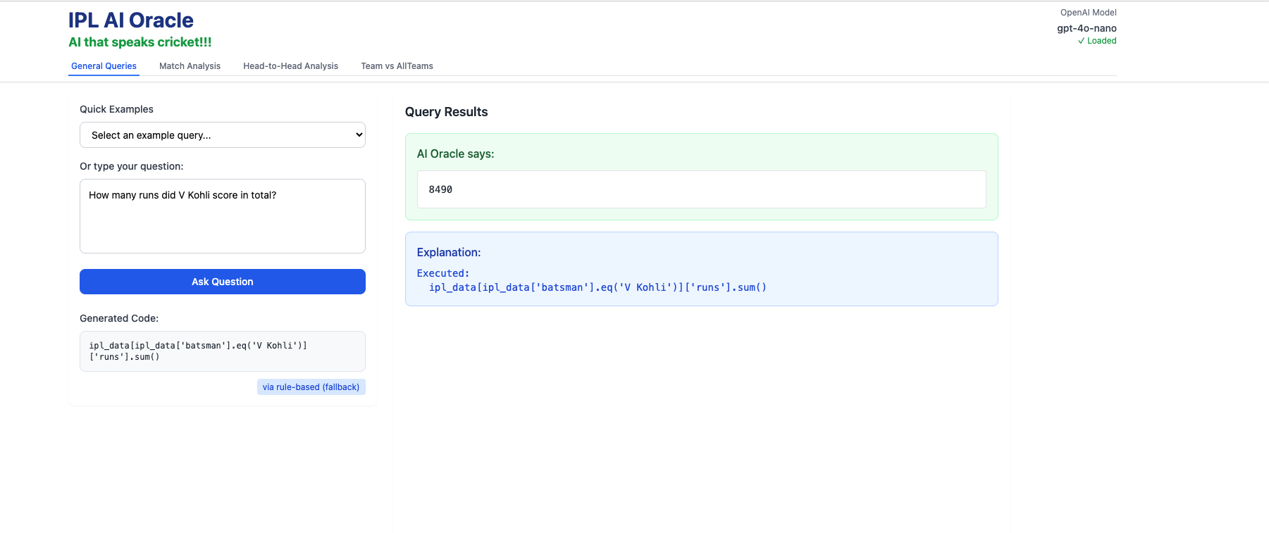
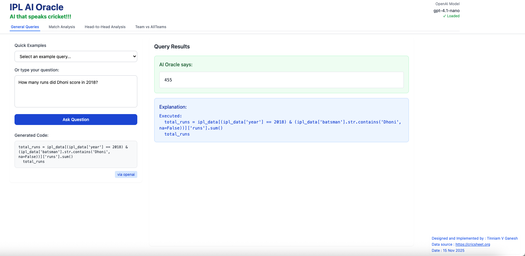
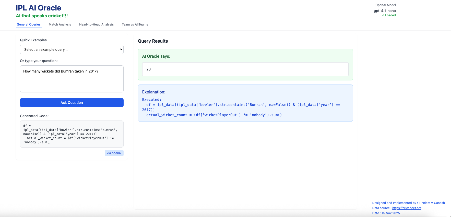
A) General Queries i) How many runs did V Kohli score in total ?
ii) How runs did MS Dhoni score in 2017?
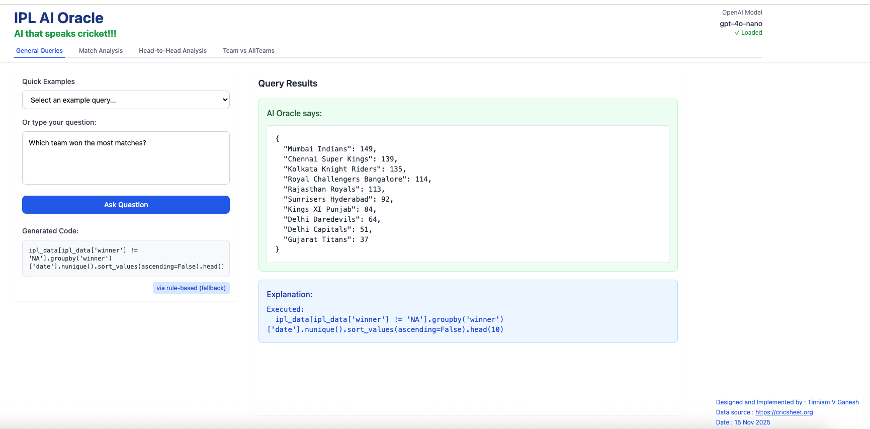
iii) Which team won the most matches?
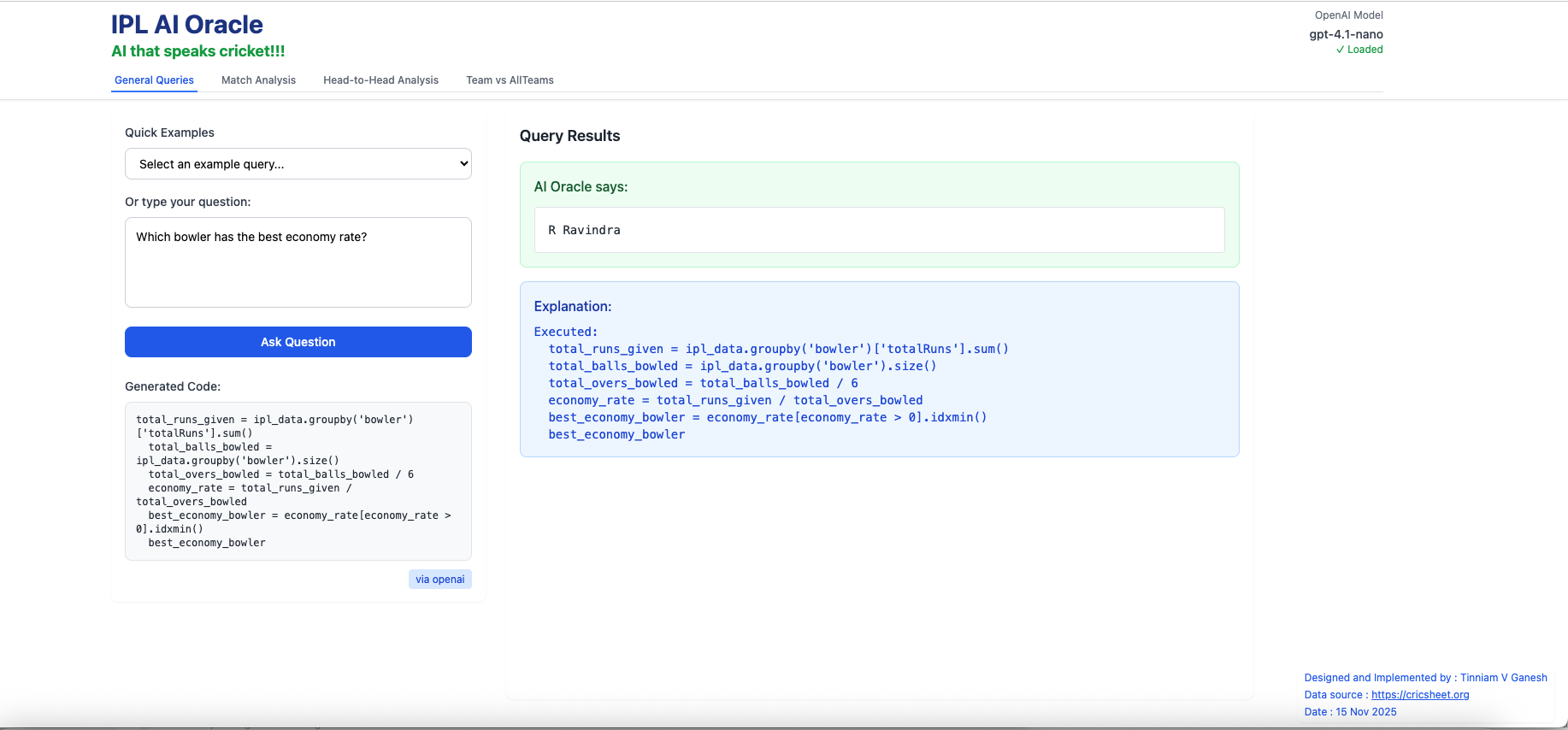
iv) Which bowler has the best economy rate?
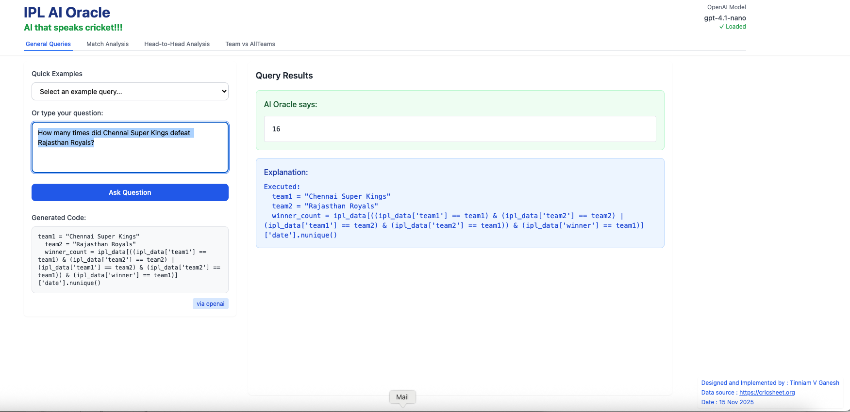
v) How many times did Chennai Super Kings defeat Rajasthan Royals?
vi) How many wickets did Bumrah take in 2017?
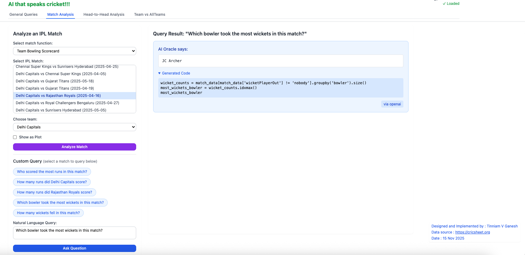
B) Match analysis – Natural Language query
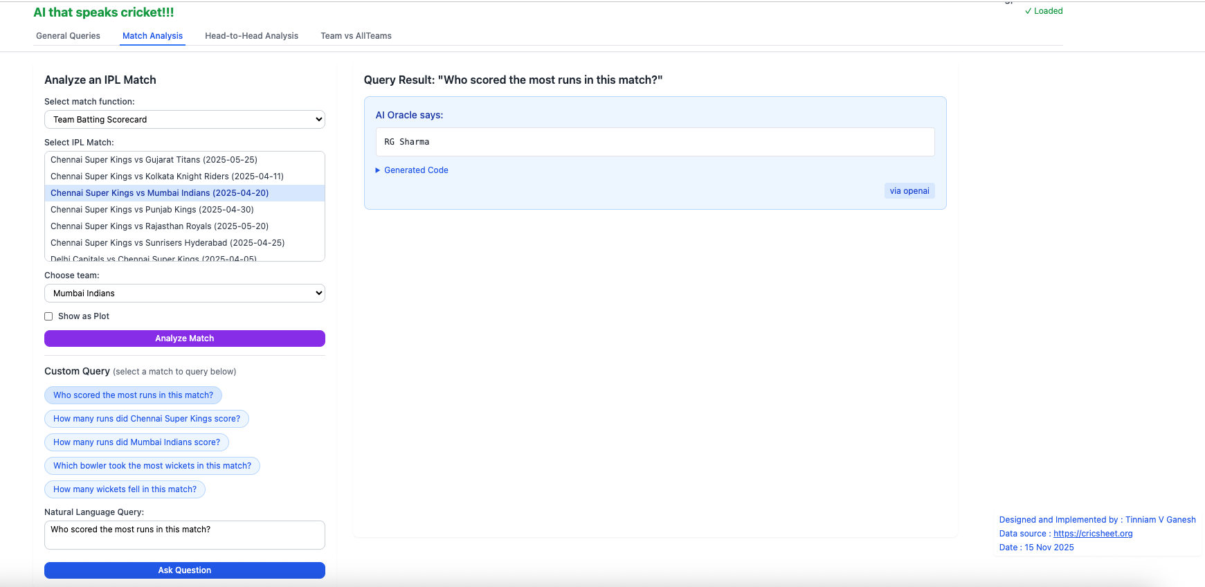
To use the Natural Language Query in this tab, you have to choose the match. For e.g.Chennai Super Kings vs Mumbai Indians (2025-04-20). Selecting a match between 2 teams will automatically create natural language chips (with red arrow). You can select any one of the chips (button) or type in your own question and click Ask Question
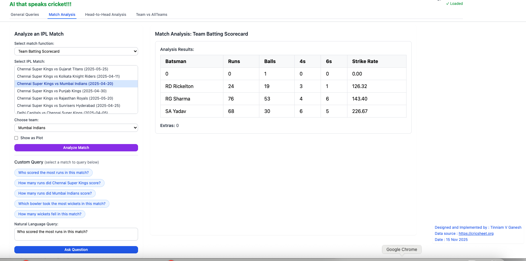
i) Who scored the most runs in this match?
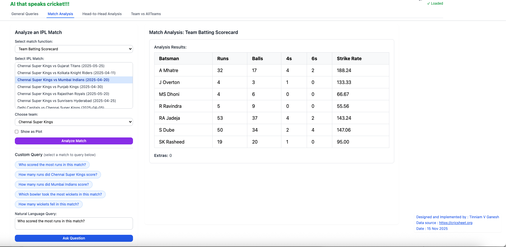
This can be verified by selecting the Batting scorecard for the match
ii) Who took the most wickets in this match?
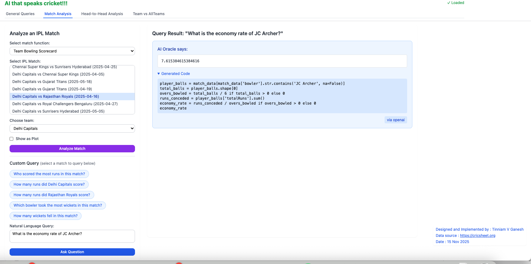
iii) What is the economy rate of JC Archer?
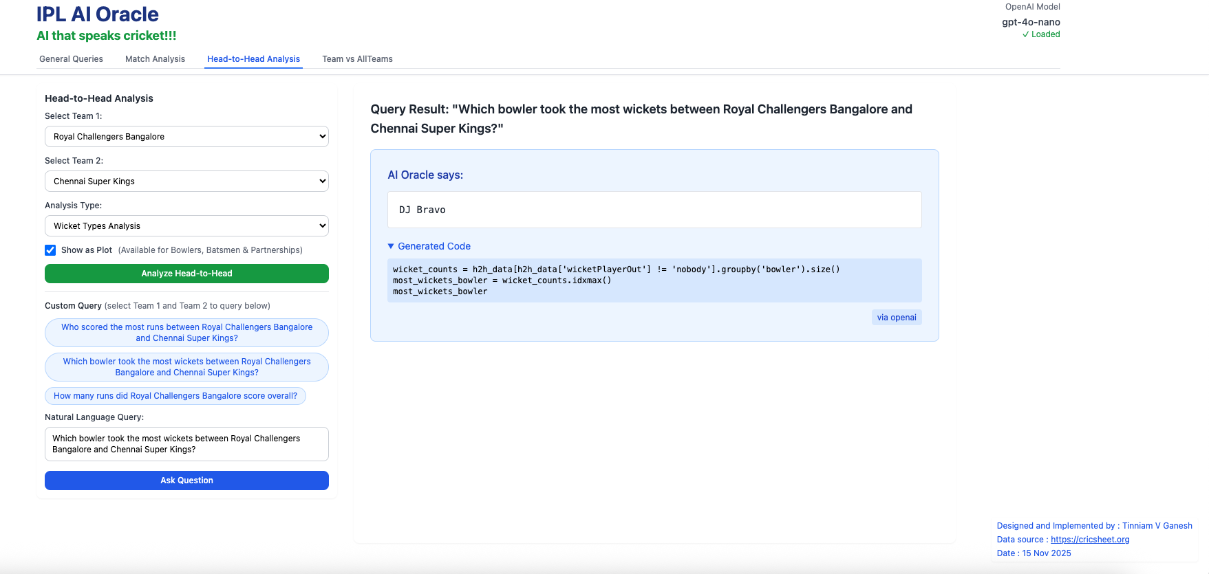
C) Head-vs-Head (Natural Language Query)
Before typing in a Natural Language Query (NLQ) ensure that Team 1 and Team 2 are selected
a) Which bowler took the most wickets between Royal Challengers Bangalore and Chennai Super Kings?
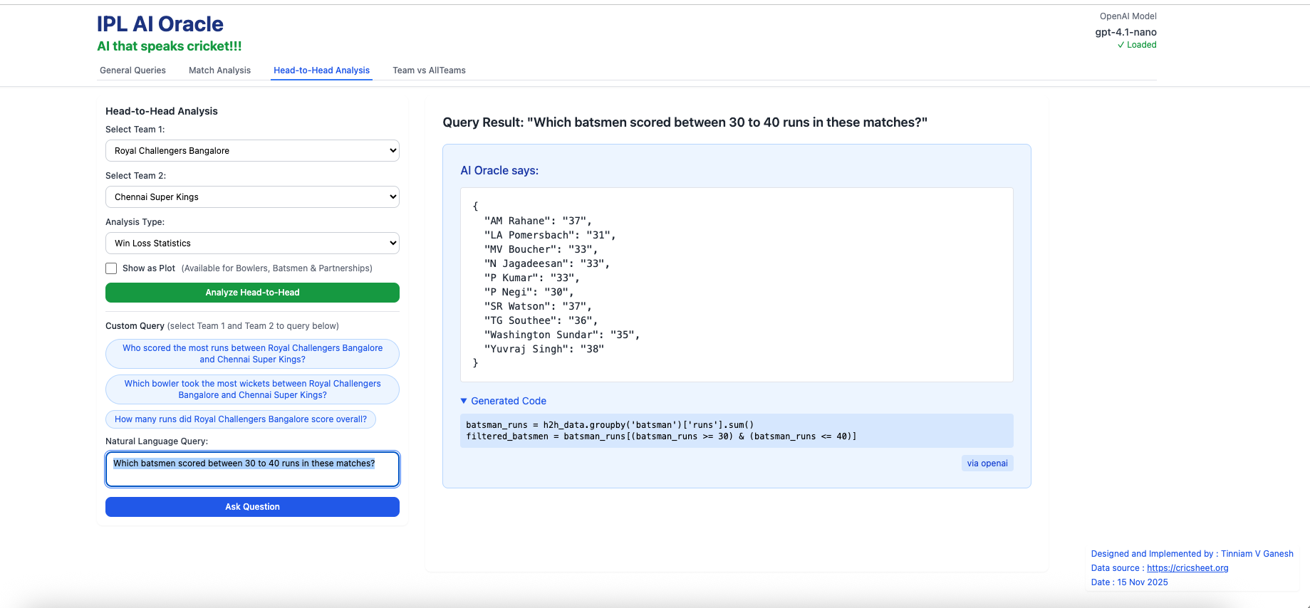
b) Which batsmen scored between 30 to 40 runs in these matches?
D) Team vs All Teams (Natural Language Query)
Remember to select the Team before using NLQ
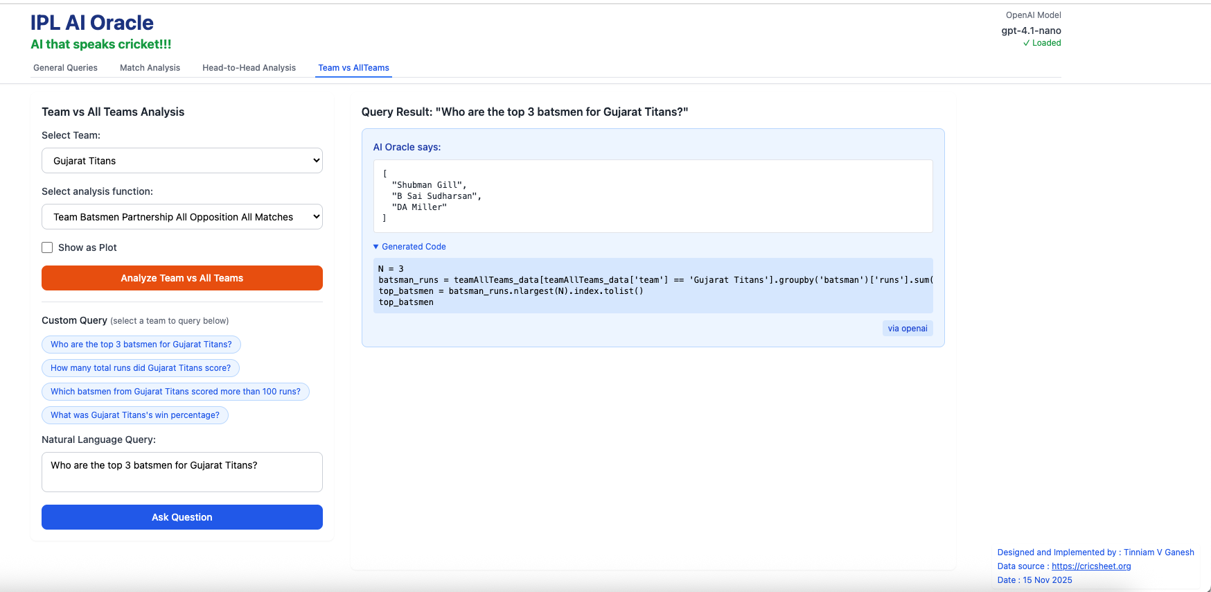
a) Who are the top 3 batsman for Gujarat Titans?
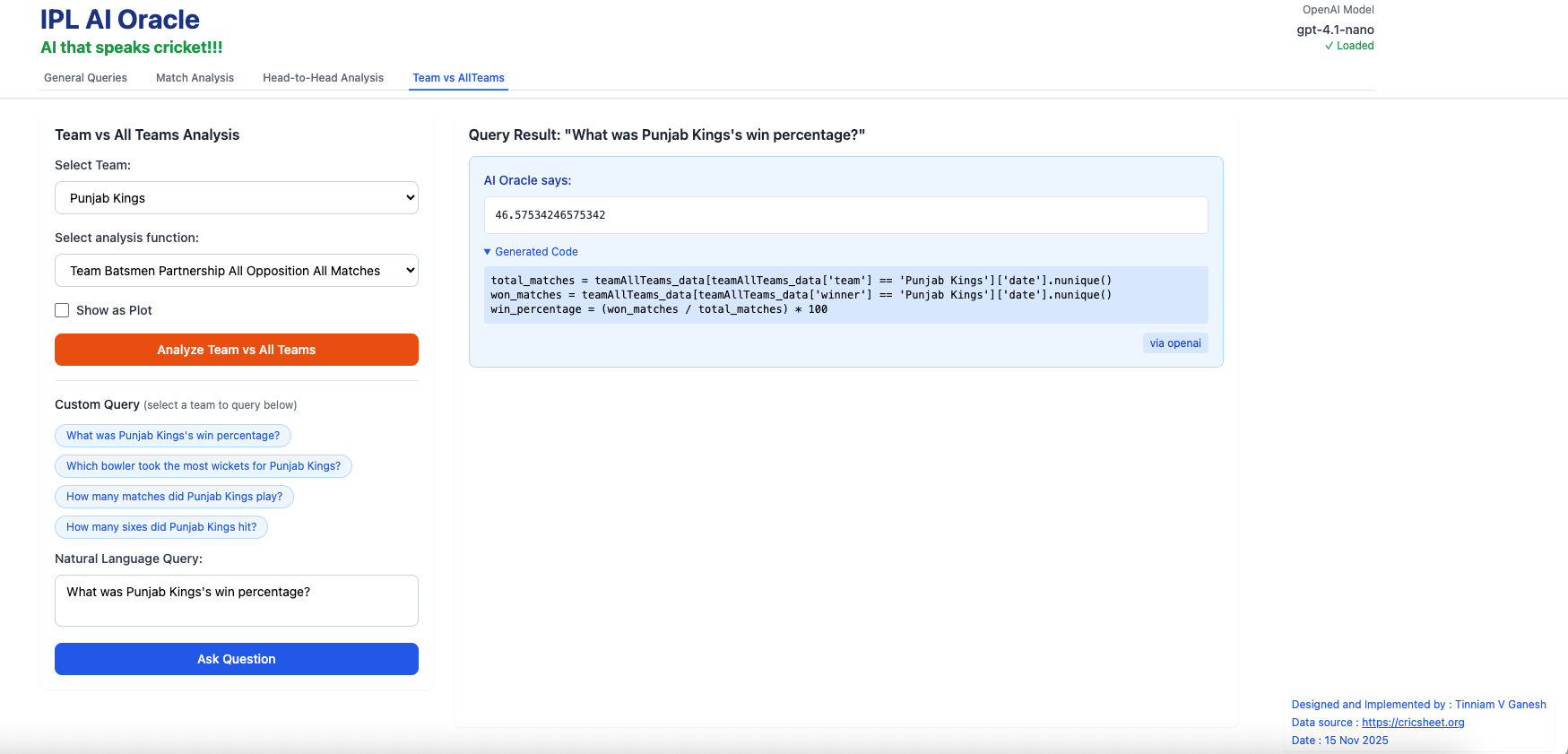
b) What was Punjab King’s win percentage?
How I Built IPL AI Oracle (with a Little Help from AI)
Here are key highlights behind the build
Data for this app comes from Cricsheet which provides ball-by-ball details in every IPL match as yaml files
Pre-processing of these yaml files were done using R utilities I already had into RData data frames, which were then subsequently converted to CSV for the different tabs
All the analytics is based on my handcoded package yorkpy as it has all the cricket rules baked in
AI assisted coding was used quite heavily for the front-end and the FastAPI backend. This was done using Cursor either with Sonnet 4.5 or GPT-5 Codex
Prompt templates for the different tabs were hand-crafted based on my package yorkpy
All-in all, the application is a healthy mix of hand-coding and AI assisted coding.
Conclusion
Since I had to deploy the application in 3 different platforms a) Vercel b) Railway c) OpenAI. I have the clock ticking in all these platforms. I initially tried gpt-4.1-mini (SLM) and then switched to gpt-4.1-nano (Tiny LM) as it is more cost effective. Since the gpt-4.1-nano has only a few hundred million parameters and is designed for low latency and cost-effectiveness, it is not as forgiving to typos or incorrect names, as some of the bigger LLMs like GPT-4o or Sonnet 4.5. Hence natural language queries work in most situations but at times they do fail. It requires quite a bit of fine-tuning I guess. Maybe work for some other day, by which time I hope the $X =N tokens/million come down drastically, so that even hobbyists like me can afford it comfortably.
Do check out IPL AI Oracle! You will get a magic link which will enable access.
“Each of us is on our own trajectory – steered by our genes and our experiences – and as a result every brain has a different internal life. Brains are as unique as snowflakes.”
David Eagleman
Introduction
The rapidly expanding wavefront of Generative AI (Gen AI), in the last couple of years, can be largely attributed to a seminal paper “Attention is all you need” by Google. This paper by Google researchers, was a landmark in the field of AI and led to an explosion of ideas and spawned an entire industry based on its theme. The paper introduces 2 key concepts a) Attention mechanism the b) Transformer Architecture. In this post, I distil the essence of Attention and Transformers.
Transformers were originally invented for Natural Language Processing (NLP) tasks like language translation, classification, sentiment analysis, summarisation, chat sessions etc. However, it led to its adaptation to languages, voice, music, images, videos etc. Prior to the advent of transformers, Natural Language Processing (NLP) was largely done through Recurrent Neural Networks (RNNs) . The problem with encoder-decoder based RNNs is that it had a fixed length for an internal-hidden state, which stored the information, for translation or other NLP tasks. Clearly, it was difficult to capture all the relevant information in this fixed length internal-hidden state. A single, final hidden state had to capture all information from the input sequence enabling it to generate the output sequence for translation and other tasks. There were some enhancements to address the shortcomings of RNNs with approaches such as Long Short-term Memory(LSTM), Gated Recurrent Unit (GRU) etc., but by and large the performance of these NLP models fell short of being reliable and consistent. This shortcoming was addressed in the paper by Bahdanau et al in the paper ‘Neural machine translation by jointly learning to align and translate‘, which discussed how ‘attention’ can be used to identify which words, align to which other words in its neighbourhood, which is computed as context vector. It implemented a ‘mechanism of attention’ by enabling the decoder to decide which parts of the sentence it needs to pay attention to, thus relieving the encoder to encode all information of the sentence into a single internal-hidden state
The attention-based transformer architecture in the paper ‘Attention is all you need‘ took its inspiration from the above Bahdanau paper and eventually evolved into the current Large Language Models (LLMs). The transformer architecture based on the attention mechanism was able to effectively address the shortcomings of the earlier RNNs. The architecture of the LLM is based on 2 key principles
a. An attention mechanism which determines the relationships between words in a sequence. It identifies how each word relates to others words in the sequence
b. A feed-forward neural network that takes the output of the attention module and enriches the relationships between the words
A final layer using softmax can predict the next word in a given sequence
LLM’s are based on the Transformer architecture. LLMs like ChatGPT, Claude, Cohere, Llama etc., typically go through 2 stages a) Pre-training b) Fine tuning
During pre-training the LLM is trained on a large corpus of unstructured text from the internet, wikipedia, arXiv, stack overflow etc. The pre-training helps the LLMs in general language understanding, enabling LLMs to learn grammar, syntax, context etc. This is followed by a fine-tuning phase where the language models is trained for specific domain or task using a smaller curated and annotated dataset of input, output pairs. This adjusts the weights of the LLM to handle the specific task in a particular domain. This may be further enhanced based on Reinforcement Learning with Human Feedback (RLHF) with reward-penalty for a given task during training. (In many ways, we humans also go through the stages of pre-training and fine-tuning in my opinion. As David Eagleman states above, we all come with a genetic blueprint based on millions of years of evolution of responses to triggers. During our early formative years this genetic DNA will create certain neural pathways in the brain akin to pre-training. Further from 2-5 years, through a couple of years of fine-tuning we learn a lot more – languages, recognition, emotion etc. This does simplify things to an extent but still I think to a large extent it holds)
Clearly, our brain is not only much more complex but also uses a minuscule energy about 60W to compute complex tasks, which is roughly equivalent to a light bulb. While for e.g. training GPT-3 which has 175 billion parameters, consumes an estimated 1287 MWH, which is roughly equivalent the consumption of an average US household for 120 years (Ref: https://adasci.org/how-much-energy-do-llms-consume-unveiling-the-power-behind-ai/?ts=1734961973)
NLP is based on the fact that human language is some ordered sequence of words. Moreover, words in a language are repetitive and thus inherently categorical. Hence, we need to use a technique for handling these categorical words for e.g. One-Hot-Encoding (OHE). But since the vocabulary of languages is extremely large, using OHE would become unmanageable. There are several other more efficient encoding methods available. Large Language Models (LLMs), which are the backbone of GenAI are trained on a large corpus of text spanning the internet, wikipedia, and other domains. The text is first converted into a numerical form through a process called tokenisation, where the words, subwords are assigned a numerical value based on some scheme. Tokenisation, can be at the character level, sub-word level, word level, sentence or even paragraph level. The choice of encoding is trade-off between vocabulary size vs sequence or context length. For character level encoding, the vocabulary will be around ~36 including letters, punctuation etc., but the sequences generated for sentences with this method will be very long. While word encodings will have a large vocabulary, an entire sentences can be captured in a shorter sequences. The encodings typically used are Byte Pair Encoding (BPE) from OpenAI, WordPiece or Sentence encoding. The sentences are first converted to tokens.
The tokens are then converted into embedding vectors which can 16, 32 or 128 real-valued dimensions. The embedding vectors convert the tokens into a multi-dimensional continuous space and capture the semantic meaning of the tokens as they get trained. The embeddings assigned, do not inherently capture the semantic meaning of words fully. But in a rough sort of way. For e.g. “I sat on the bank of a river” and “I deposited money in a bank”, the word bank may have the same embedding. But as the model is trained through the transformer with sequences of text passing through the attention module, the embeddings are updated with contextual information. So for e.g. in the 1st sentence “bank” will be associated with the word “river” and in the 2nd sentence the attention module will also capture the context of the “bank” and associate it with the word “money”
A transformer is well suited for predicting the next word in a given sequence. This is called a auto-regressive decoder-only model. The sequence of steps a enable a Transformer to be capable of predicting the next word in a given sequence is based on the following steps
a) Training on a large corpus of text from internet, wikipedia, books, and research repositories like arXiv etc
The text are tokenised based on one of the tokenisation schemes mentioned above like BPE, Wordpiece etc. to convert the words into numerical values
The tokens are then converted into multi-dimensional real-valued embedding vectors. The embeddings are vectors which through multiple iterations capture richer meaning context-aware meaning of sentences
The Attention module determines the affinity each word has to the other words in the sentence. This affinity can be captured over longer sentence structures too and this is based on the context (sequence) length depending on the size of the model.
The weights from the output of the Attention module then go to a simple 2 layer Feed Forward Neural Network (FFN) which tries to predict the next word in a sentence. For this each sentence is taken as input with the target being the same sentence shifted by one place.
For e,g,
Input: Mary had a little lamb
Target: had a little lamb <end>
So in a sentence w1 , w2, w3, … , wn the FFN will use
w1 to predict w2
w1 , w2 to predict w3 and so on During back propagation, the error between the predicted word and the actual target word is calculated and propagated backwards through the network updating the weights and biases of the NN. The FFN uses tries to minimise the cross-entropy or log loss which computes the difference between the predicted probabilities and target values.
Attention module
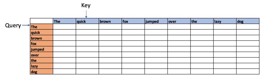
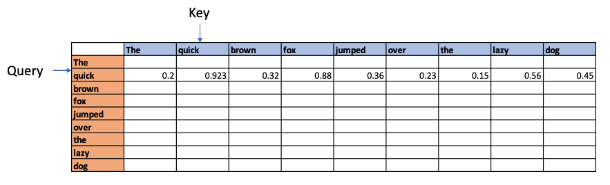
For e.g. if we had the sentence “The quick brown fox jumped over the lazy dog”, Attention is computed as follows
Each word in the above sentence is tokenised and represented as dense vector. The transformer architecture uses 3 weight matrices call Wq , Wk, Wv called the Query Weight, Key Weight and Value weight matrices which are learnable matrices. The embedding vectors of the sentence are multiplied with these Wq, Wk, Wv matrices to give Q (Query), K(Key) and V (Value) vectors.
The dot product of the Query vector with all the Key vectors is performed. Since these are vectors, the dot product will determine the similarity or alignment, the query ‘The’ has for the each of the Keys. This is the fundamental concept of of the Attention module. This is because in a multi-dimensional vector space, vectors which are closer together will give a high dot product. Hence, the dot product between the Query and all the Keys gives the affinity the Query has to all other Keys. This is computed as the Attention Score.
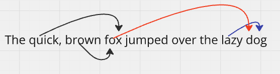
For e,g the above process could show that quick and brown attend to the fox, and lazy attends to the dog – and they have relatively high Attention Scores compared to the rest. In addition the Attention operation may also determine that there is a relation between fox and dog in the sentence.
These affinities show up over several iterations through batches of sentences as Wq, WK, Wv are learnable parameters. The relationship learned is depicted below
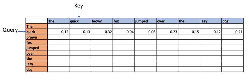
Next the values are normalised using the Softmax function since this will result in a mean of 0 and a variance of 1. This will give normalised attention scores
Causal attention. Since future words cannot affect the earlier words these values are made -Infinity so when we perform Softmax we get the value 0 for these values
Self-Attention Mechanism enables the model to evaluate the importance of tokens relative to each other. The self-attention mechanism is written as
where Q, K, V are Query, Key and Value vectors and dK is the dimensionality of the Key vectors. scales the dot product so that the dot product values are not overly large
where the Scaled Attention score =
The Attention weights = softmax(Scaled Attention score)
This computes a context-aware representation of each token with respect to all other tokens
Feed Forward Network (FFN)
In the case of training a language model the fact that language is sequential enables the model to be trained on the language itself. This is done by training the model on large corpus of text, where the language learns to predict the next words in the sequence. So for example in the sentence
Feedforward Network (FFN) comprises two linear transformations separated by a non-linearity, typically modeled
with the first layer transformation as
and the second layer transformation is
where and are the weight matrices, and and are the biases
where x and
x and is usually 4 times the dimesnion of
is the activation function which can be ReLU, GELU or SwiGLU
Input to the FFN
The Decoder receives the output of the Self Attention module to the FFN network. This output from the Attention module is context-aware with the words in the input sequence having different affinities to other words in the sequence
The Target of the FFN is the input sequence shifted by one word
The output from the Attention head and the layer normalization
Normed Output = LayerNorm(Input+MultiHeadOutput)
In essence the Decoder only architecture can be boiled down to the following main modules
Tokenization – The input text is split either on characters, subwords, words, to convert the text into numbers
Vector Embedding – The numerical tokens are then converted into Dense vectors
Positional Embedding – The position order of the text sequence is encoded using the positional embedding. This positional embedding is added to the vector embedding
Attention module – The attention module computes the affinity the different words have for other words in its vicinity. This is done through the the use of 3 weight matrices , , . By multiplyting these matrices with the input vectors we get Q,K and V vectors. The attention is computed as
For the decoder, attention is masked to prevent the model from looking at future tokens during training also known as causal attention mentioned above
The output pf the Attention module is passed to a 2 layer FFN which uses GeLU activation with Adam optimszation. This involves the following 2 steps
Computing the cross-entropy (loss) using the predicted words and the actual labels
Backpropagting the error through all the layers and updating the layer weights,
If the size of the FFN’s output is the vocabulary size then we can use P(next word|context)=softmax(FFN output) If the size of the model output is not the vocabulary size then the a final linear layer embeds the output to the size of the dictionary. This maps the model’s hidden states to the vocabulary size enabling the predicting of the next word from the vocabulary
Next word prediction : The next word prediction is done by applying softmax on the output of the FFN layer (logits) to compute the probability for the vocabulary
P(next word∣context)=softmax(Logits)
After computing the probability the model selects the next word based on one of many options – to either choose the most probable word or on some other algorithm
The above sequence of steps is a bare-bones attention and transformer module. In of itself it can achieve little as the transformer module will have to contend with vanishing or exploding gradient issues. It needs additional bells and whistles to make it work effectively
Additional layers to the above architecture
a) Residual Connection and Layer Normalisation (Add + Norm) –
i) Residual, skip connections
Residual connection or skip connections are added the input of each layer to the output to enable the gradients to propagate effectively. This is based on the paper ‘Deep Residual Learning for Image Recognition” from Microsoft
Residual connections also known as skip or shortcut connections are performed by adding the input of layer to the output of the layer as a shortcut. This helps in preventing the vanishing gradient, because of the gradients become progressively smaller as they pass through successive layers.
ii) Layer normalisation
In addition layer normalisation is done to stabilise the activation across a single feature to have 0 mean and a variance of 1 by computing
Mean and variance calculation
,
Normalization
Layer normalization introduces learnable parameters using the equation
This can be written as ResidualOutput=Input+Output of Attention/FFN
The above statement mentions that the Input layer to the Attention /FFN module is added to the output to mitigate the vanishing gradient problem
NormedOutput=LayerNorm(Residual Output)
Layer Normalisation is then applied to the Residual Output to stabilise the activations.
b) Multi-headed Attention : Typically Transformer use multiple parallel heads of attention. Each head will compute a slightly different variations to the attention values, thus making the whole learning process richer. Multi-headed learning is capable of capturing more nuanced affinities of different words in the sentence to other words in the sentence/context.
c) Dropout : Dropout is a technique where random hidden units or neurons are dropped from the network during training. This prevents overfitting and helps to regularise/generalise the learning of the network. In Transformer Architectures, dropout is used after calculating the Attention Weights. Dropout can also be applied in the Feed Forward Network or in the Residual Connections
This is shown diagrammatically here
Points to note:
a) The Attention mechanism is able to pick out affinities between words in a sentence. This happens despite the fact the the WQ, WK, WV matrices are randomly initialised. As the model trained iteratively through a large corpus of text using next token prediction for Auto Regressive Transformers and Masked prediction as in the case of BERT, then the affinities show up. This training allows the model to learn the contextual relationships and affinities words have with each other. The dot product Q, K measures the affinity words have for each other and will be high if they are highly related to each other. This is because they will aligned in a the multi-dimensional embedding space of these vectors, besides semantically and contextually related tokens are closer to each other.
b) The Feed Forward Network (FFN) in the Transformer’s Attention block is relatively small and has just 2 layers. This is for computational efficiency and deeper Neural Networks can increase costs. Moreover, it has been found that deeper and wider networks did not significantly improve performance while also preventing overfitting.
c) The above architecture is based on the Causal Attention, Decoder only transformer. The original paper includes both the encoder and the decoder to enable translation across different languages. In addition architectures like BERT use ‘masked attention’ and randomly mask words
The flow of vectors and dimensionality from the input sentence tokens to the output token prediction is as follows
a) For a batch (B) of 2 sentences with 6 words (T) each, where each word is converted into a token. If Byte Pair Encoding (BPE) is used then an integer value between 1-50257 will be obtained.
Input shape = (B x T) = (2 x 6)
b) Token embedding – Each token in the vocabulary is converted into an embedding vector of size = 512 dimension vector
Output shape = (B x T x ) = (2 x 6 x 512)
c) Positional embedding is added
Shape of positional embedding = T x = (6 x512)
d) Output shape with token and positional embedding is the same
Output shape = (B x T x ) = (2 x 6 x 512)
d) Multi-head attention
e) The WQ, WK, WV learnable matrices are each of size
x
f) Q = X x WQ = (B x T x ) x ( x )
Output shape of Q, K, V = (B x T x ) = (2 x 6 x 512)
g) Number of heads h = 8
Dimensionality of each head = /8 = = 64
h) Splitting across the heads we have
Shape per head = (B, h, T, ) = ( 2, 8, 6, 64)
h) Weighted sum of values =
Output shape per head = (B, h, T, ) = ( 2, 8, 6, 64)
i) All the heads are concatenated
(B x T x ) = (2 x 6 x 512)
j) The FFN has one hidden layer which is 4 times
= x 4
Final output of FFN after passing through hidden layer and back
Output shape =(B x T x ) = (2 x 6 x 512)
k) Residual, shortcut connections and layer norm do not change shape
Output shape =(B x T x ) = (2 x 6 x 512)
l) The final output is projected back into the original vocabulary space. For BPE it
50257.
Using a weight matrix (512 x vocab_size) = (512 x 50257)
Final output shape = (B x T x vocab_size) = (2 x 6 x 50257)
The output is in probabilities and hence gives the most likely next word in the sentence
Conclusion
This post tries to condense the key concepts around the Attention mechanism and the Transformer Architecture which have been the catalyst in the last few years, resulting in an explosion in the area of Gen AI, and there seems to be no stopping. It is indeed fascinating how the human language has been mathematically analysed for semantic meaning and relevance.
Often times before crucial matches, or in general, we would like to know the performance of a batsman against a bowler or vice-versa, but we may not have the data. We generally have data where different batsmen would have faced different sets of bowlers with certain performance data like ballsFaced, totalRuns, fours, sixes, strike rate and timesOut. Similarly different bowlers would have performance figures(deliveries, runsConceded, economyRate and wicketTaken) against different sets of batsmen. We will never have the data for all batsmen against all bowlers. However, it would be good estimate the performance of batsmen against a bowler, even though we do not have the performance data. This could be done using collaborative filtering which identifies and computes based on the similarity between batsmen vs bowlers & bowlers vs batsmen.
This post shows an approach whereby we can estimate a batsman’s performance against bowlers even though the batsman may not have faced those bowlers, based on his/her performance against other bowlers. It also estimates the performance of bowlers against batsmen using the same approach. This is based on the recommender algorithm which is used to recommend products to customers based on their rating on other products.
This idea came to me while generating the performance of batsmen vs bowlers & vice-versa for 2 IPL teams in this IPL 2022 with my Shiny app GooglyPlusPlus in the optimization tab, I found that there were some batsmen for which there was no data against certain bowlers, probably because they are playing for the first time in their team or because they were new (see picture below)
In the picture above there is no data for Dewald Brevis against Jasprit Bumrah and YS Chahal. Wouldn’t be great to estimate the performance of Brevis against Bumrah or vice-versa? Can we estimate this performance?
While pondering on this problem, I realized that this problem formulation is similar to the problem formulation for the famous Netflix movie recommendation problem, in which user’s ratings for certain movies are known and based on these ratings, the recommender engine can generate ratings for movies not yet seen.
This post estimates a player’s (batsman/bowler) using the recommender engine This post is based on R package recommenderlab
You can download this R Markdown file and the associated data and perform the analysis yourself using any other recommender engine from Github at playerPerformanceEstimation
Problem statement
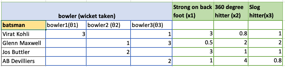
In the table below we see a set of bowlers vs a set of batsmen and the number of times the bowlers got these batsmen out. By knowing the performance of the bowlers against some of the batsmen we can use collaborative filter to determine the missing values. This is done using the recommender engine.
The Recommender Engine works as follows. Let us say that there are feature vectors , and for the 3 bowlers which identify the characteristics of these bowlers (“fast”, “lateral drift through the air”, “movement off the pitch”). Let each batsman be identified by parameter vectors , and so on
For e.g. consider the following table
Then by assuming an initial estimate for the parameter vector and the feature vector xx we can formulate this as an optimization problem which tries to minimize the error for This can work very well as the algorithm can determine features which cannot be captured. So for e.g. some particular bowler may have very impressive figures. This could be due to some aspect of the bowling which cannot be captured by the data for e.g. let’s say the bowler uses the ‘scrambled seam’ when he is most effective, with a slightly different arc to the flight. Though the algorithm cannot identify the feature as we know it, but the ML algorithm should pick up intricacies which cannot be captured in data.
Hence the algorithm can be quite effective.
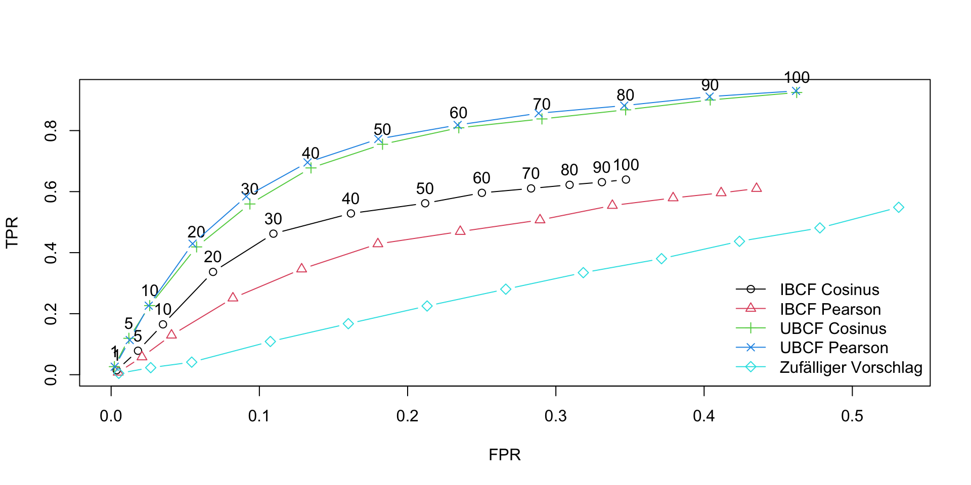
Note: The recommender lab performance is not very good and the Mean Square Error is quite high. Also, the ROC and AUC curves show that not in aLL cases the algorithm is doing a clean job of separating the True positives (TPR) from the False Positives (FPR)
Note: This is similar to the recommendation problem
The collaborative optimization object can be considered as a minimization of both and the features x and can be written as
J(, }= 1/2
The collaborative filtering algorithm can be summarized as follows
Initialize , … and the set of features be ,, … , to small random values
Minimize J(, … ,, , … ,) using gradient descent. For every j=1,2, …, i= 1,2,..,
:= – ( ) –
&
:= – (
Hence for a batsman with parameters and a bowler with (learned) features x, predict the “times out” for the player where the value is not known using
The above derivation for the recommender problem is taken from Machine Learning by Prof Andrew Ng at Coursera from the lecture Collaborative filtering
There are 2 main types of Collaborative Filtering(CF) approaches
User based Collaborative Filtering User-based CF is a memory-based algorithm which tries to mimics word-of-mouth by analyzing rating data from many individuals. The assumption is that users with similar preferences will rate items similarly.
Item based Collaborative Filtering Item-based CF is a model-based approach which produces recommendations based on the relationship between items inferred from the rating matrix. The assumption behind this approach is that users will prefer items that are similar to other items they like.
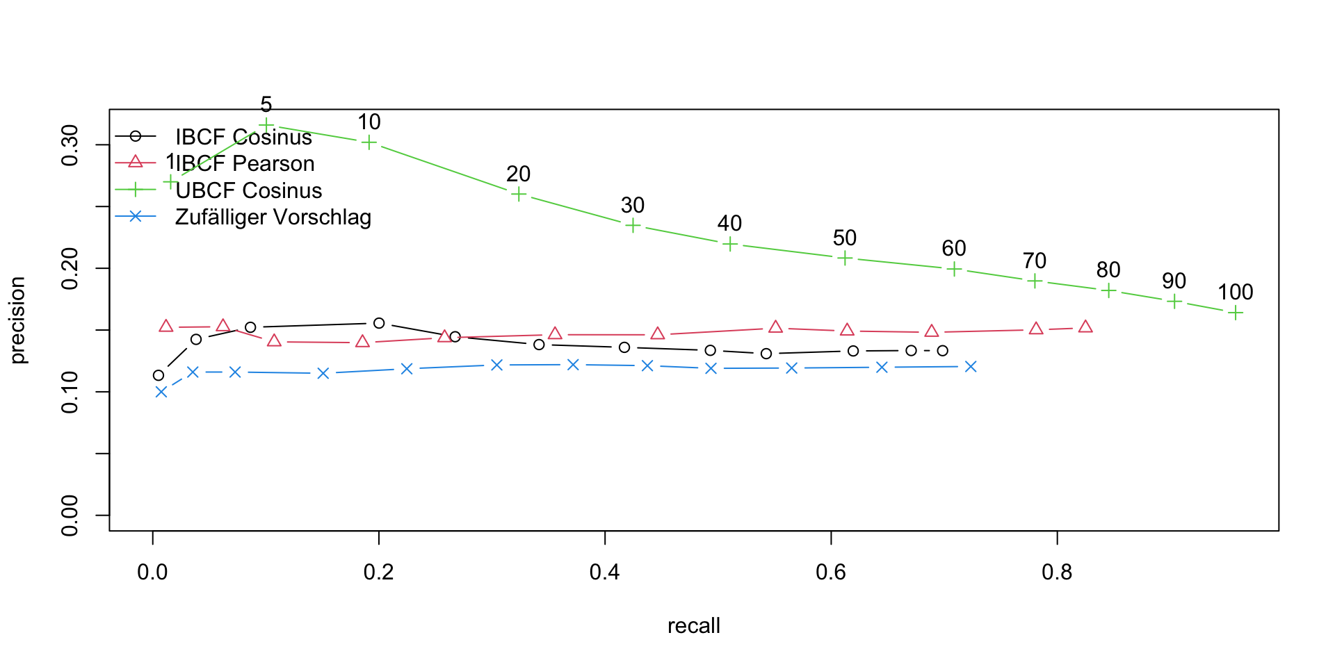
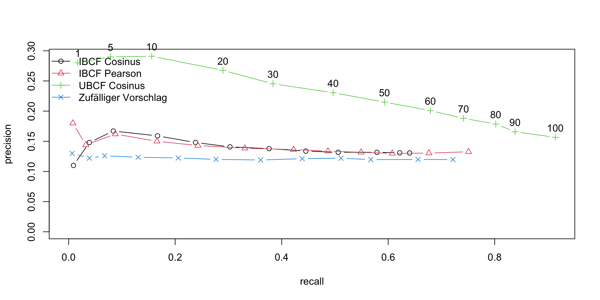
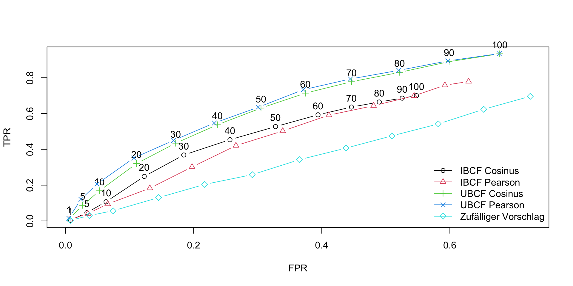
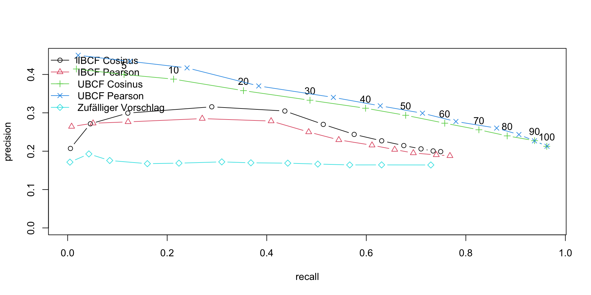
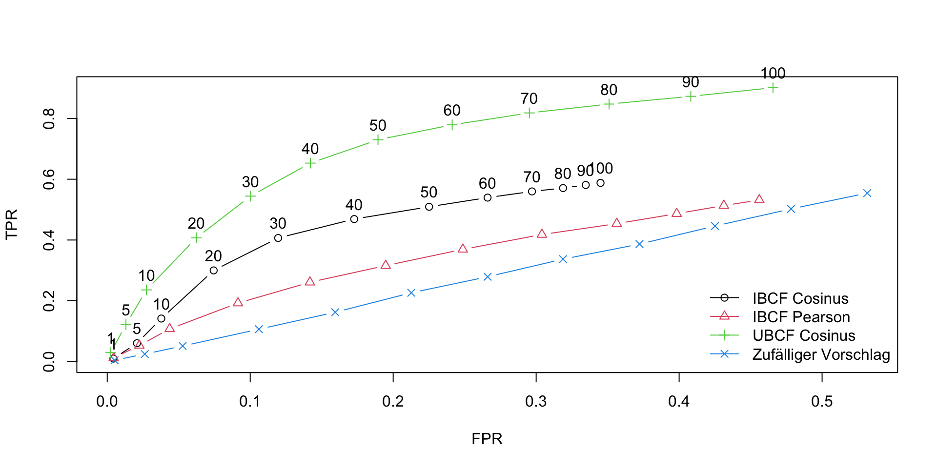
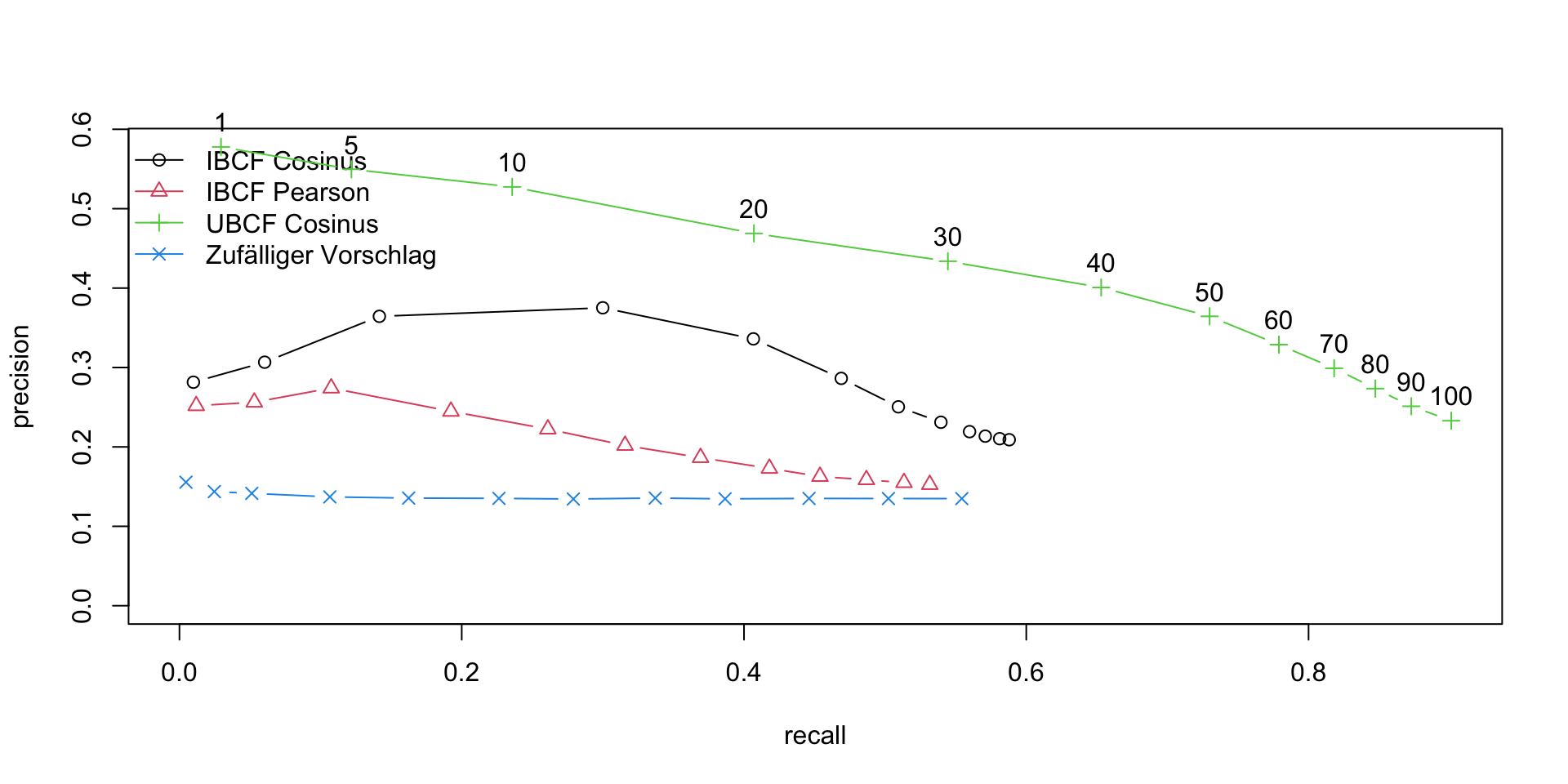
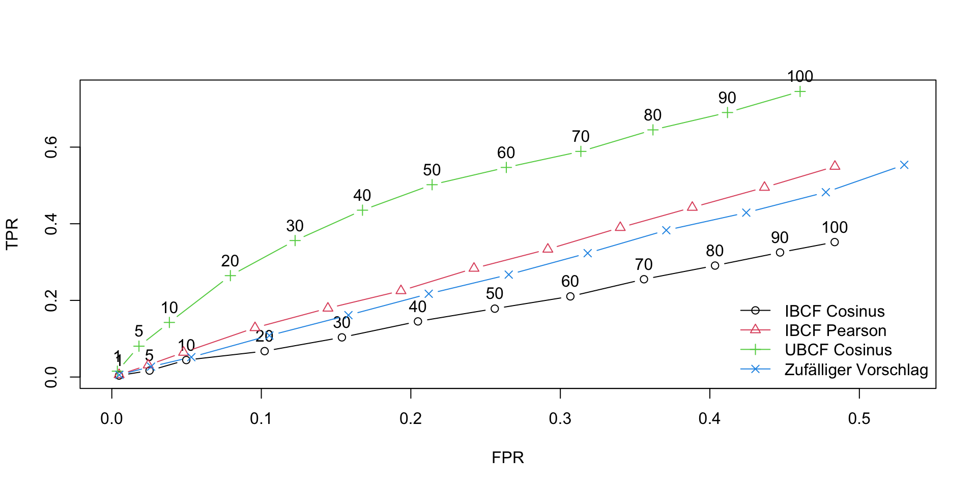
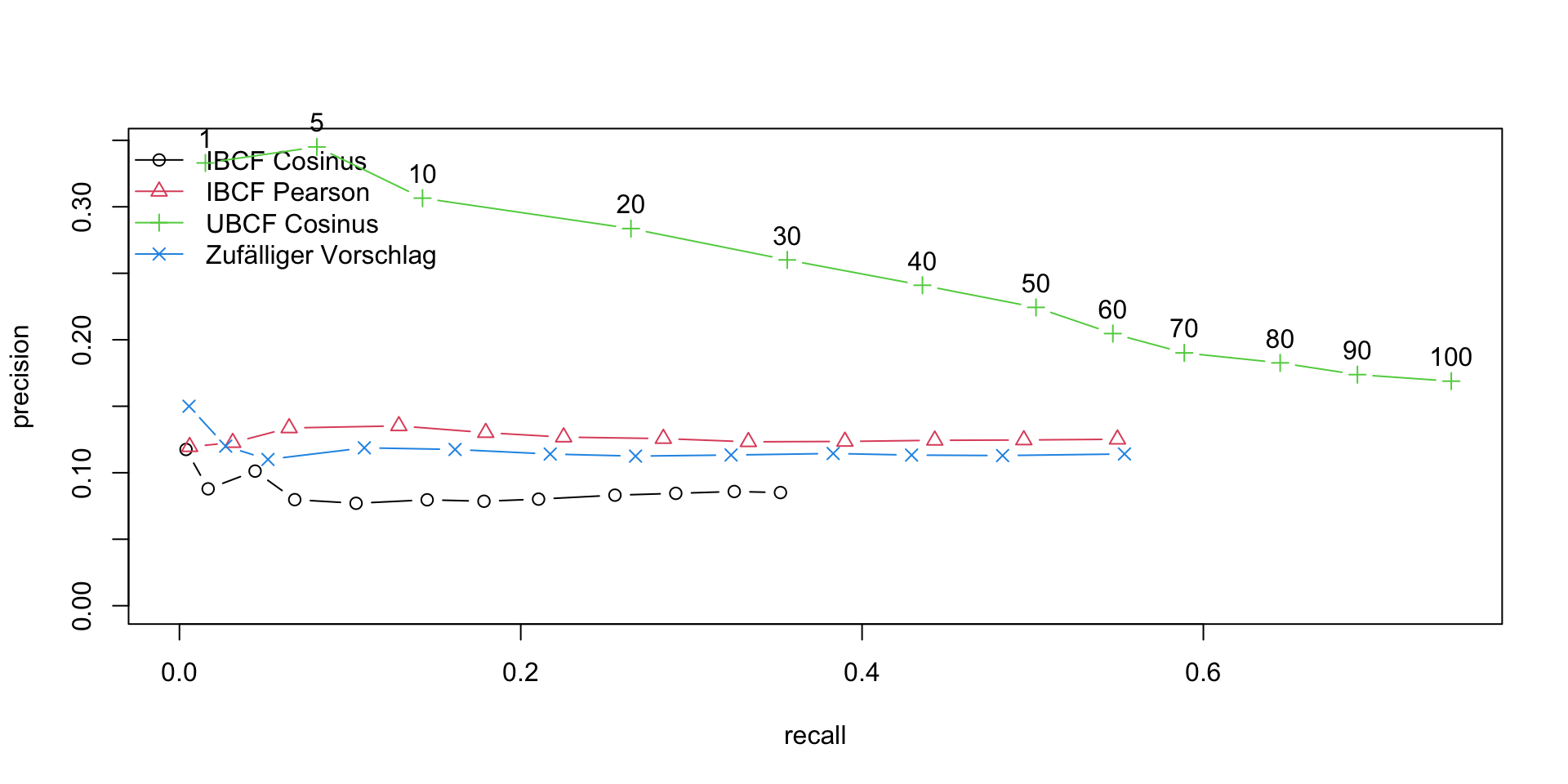
1a. A note on ROC and Precision-Recall curves
A small note on interpreting ROC & Precision-Recall curves in the post below
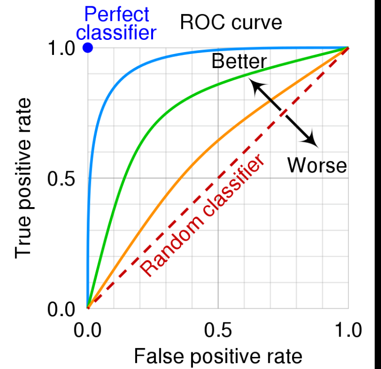
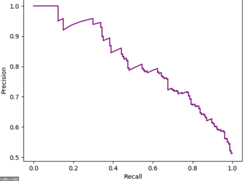
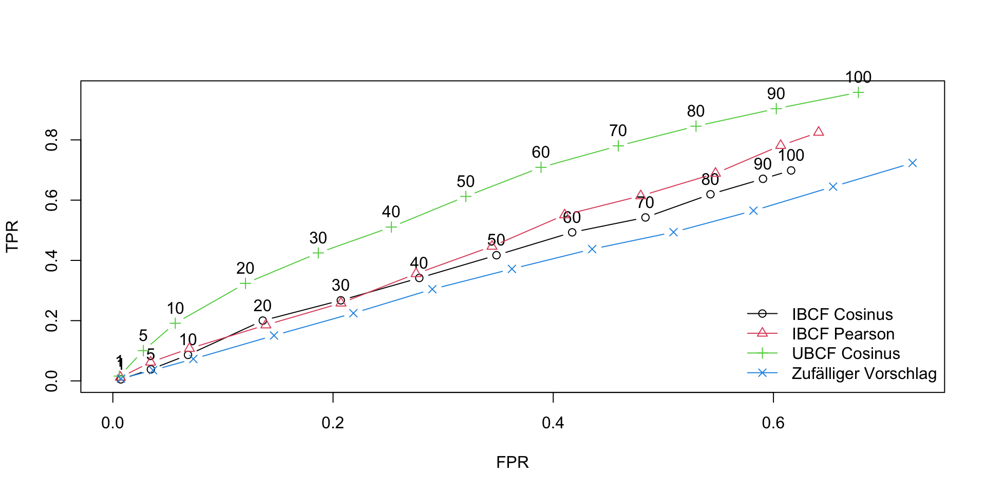
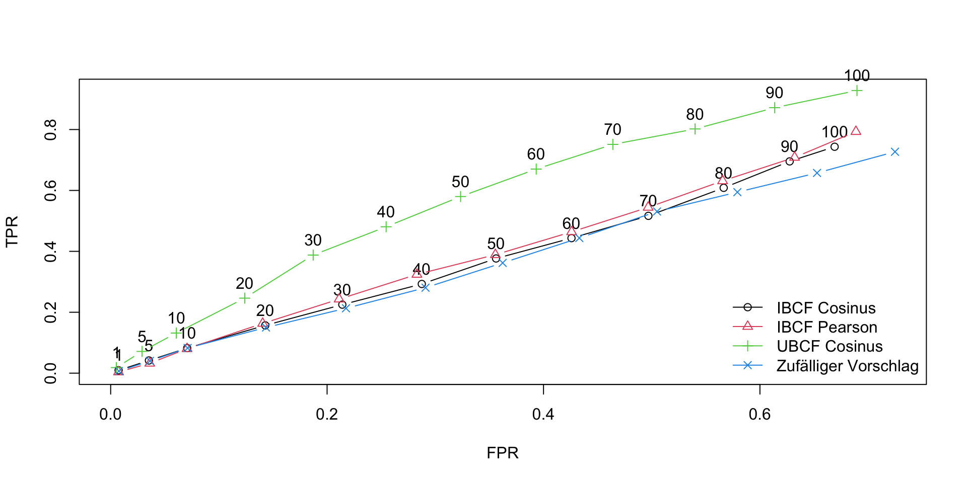
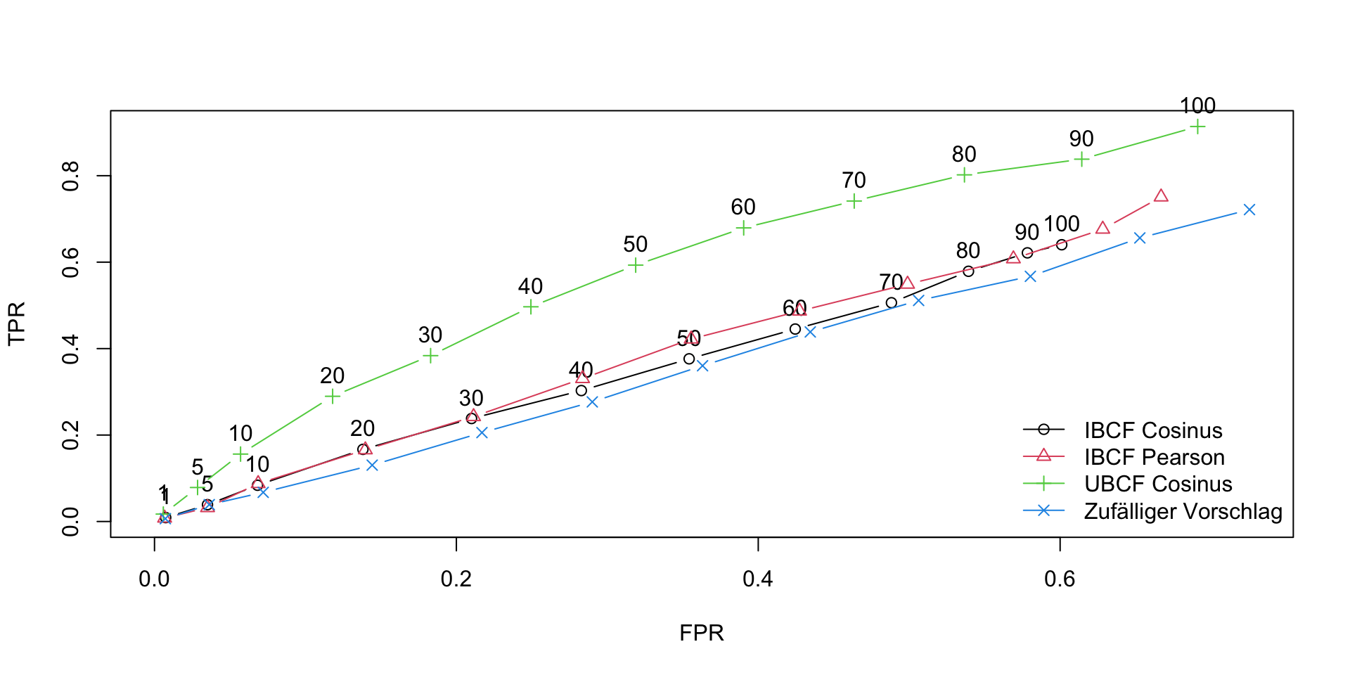
ROC Curve: The ROC curve plots the True Positive Rate (TPR) against the False Positive Rate (FPR). Ideally the TPR should increase faster than the FPR and the AUC (area under the curve) should be close to 1
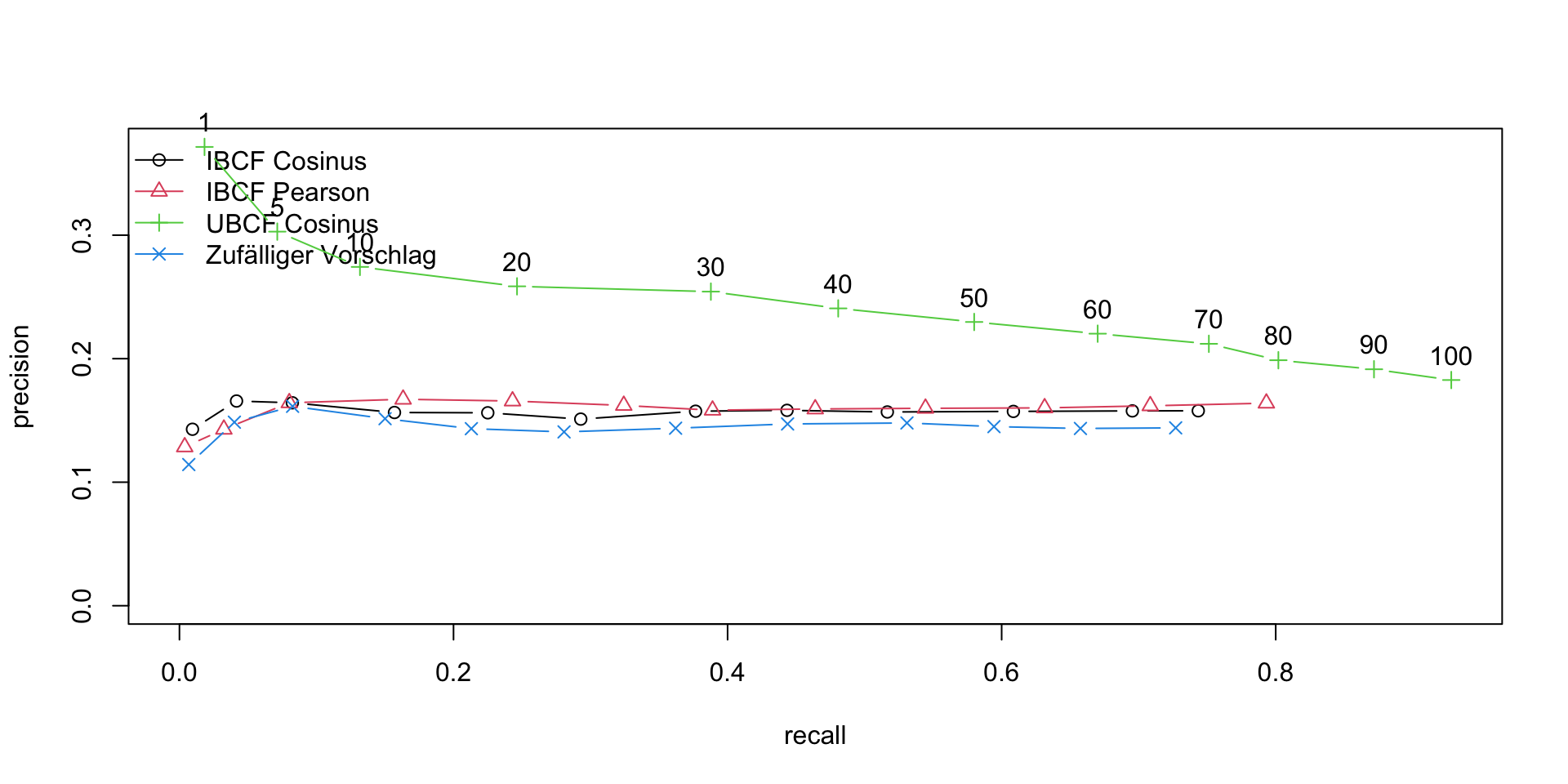
Precision-Recall: The precision-recall curve shows the tradeoff between precision and recall for different threshold. A high area under the curve represents both high recall and high precision, where high precision relates to a low false positive rate, and high recall relates to a low false negative rate
Helper functions for the RMarkdown notebook are created
eval – Gives details of RMSE, MSE and MAE of ML algorithm
evalRecomMethods – Evaluates different recommender methods and plot the ROC and Precision-Recall curves
# This function returns the error for the chosen algorithm and also predicts the estimates
# for the given data
eval <- function(data, train1, k1,given1,goodRating1,recomType1="UBCF"){
  set.seed(2022)
  e<- evaluationScheme(data,
                       method = "split",
                       train = train1,
                       k = k1,
                       given = given1,
                       goodRating = goodRating1)

  r1 <- Recommender(getData(e, "train"), recomType1)
  print(r1)

  p1 <- predict(r1, getData(e, "known"), type="ratings")
  print(p1)

  error = calcPredictionAccuracy(p1, getData(e, "unknown"))

  print(error)
  p2 <- predict(r1, data, type="ratingMatrix")
  p2
}
# This function will evaluate the different recommender algorithms and plot the AUC and ROC curves
evalRecomMethods <- function(data,k1,given1,goodRating1){
  set.seed(2022)
  e<- evaluationScheme(data,
                       method = "cross",
                       k = k1,
                       given = given1,
                       goodRating = goodRating1)

  models_to_evaluate <- list(
    `IBCF Cosinus` = list(name = "IBCF",
                          param = list(method = "cosine")),
    `IBCF Pearson` = list(name = "IBCF",
                          param = list(method = "pearson")),
    `UBCF Cosinus` = list(name = "UBCF",
                          param = list(method = "cosine")),
    `UBCF Pearson` = list(name = "UBCF",
                          param = list(method = "pearson")),
    `Zufälliger Vorschlag` = list(name = "RANDOM", param=NULL)
  )

  n_recommendations <- c(1, 5, seq(10, 100, 10))
  list_results <- evaluate(x = e,
                           method = models_to_evaluate,
                           n = n_recommendations)
  plot(list_results, annotate=c(1,3), legend="bottomright")
  plot(list_results, "prec/rec", annotate=3, legend="topleft")
}
3. Batsman performance estimation
The section below regenerates the performance for batsmen based on incomplete data for the different fields in the data frame namely balls faced, fours, sixes, strike rate, times out. The recommender lab allows one to test several different algorithms all at once namely
User based – Cosine similarity method, Pearson similarity
Item based – Cosine similarity method, Pearson similarity
Popular
Random
SVD and a few others
3a. Batting dataframe
head(df)
##   batsman1         bowler1 ballsFaced totalRuns fours sixes  SR timesOut
## 1 A Badoni        A Mishra          0         0     0     0 NaN        0
## 2 A Badoni        A Nortje          0         0     0     0 NaN        0
## 3 A Badoni         A Zampa          0         0     0     0 NaN        0
## 4 A Badoni     Abdul Samad          0         0     0     0 NaN        0
## 5 A Badoni Abhishek Sharma          0         0     0     0 NaN        0
## 6 A Badoni      AD Russell          0         0     0     0 NaN        0
3b Data set and data preparation
For this analysis the data from Cricsheet has been processed using my R package yorkr to obtain the following 2 data sets – batsmenVsBowler – This dataset will contain the performance of the batsmen against the bowler and will capture a) ballsFaced b) totalRuns c) Fours d) Sixes e) SR f) timesOut – bowlerVsBatsmen – This data set will contain the performance of the bowler against the difference batsmen and will include a) deliveries b) runsConceded c) EconomyRate d) wicketsTaken
Obviously many rows/columns will be empty
This is a large data set and hence I have filtered for the period > Jan 2020 and < Dec 2022 which gives 2 datasets a) batsmanVsBowler20_22.rdata b) bowlerVsBatsman20_22.rdata
I also have 2 other datasets of all batsmen and bowlers in these 2 dataset in the files c) all-batsmen20_22.rds d) all-bowlers20_22.rds
##                 A Mishra A Nortje A Zampa Abdul Samad Abhishek Sharma
## A Badoni              NA       NA      NA          NA              NA
## A Manohar             NA       NA      NA          NA              NA
## A Nortje              NA       NA      NA          NA              NA
## AB de Villiers        NA        4       3          NA              NA
## Abdul Samad           NA       NA      NA          NA              NA
## Abhishek Sharma       NA       NA      NA          NA              NA
## AD Russell             1       NA      NA          NA              NA
## AF Milne              NA       NA      NA          NA              NA
## AJ Finch              NA       NA      NA          NA               3
## AJ Tye                NA       NA      NA          NA              NA
##                 AD Russell AF Milne AJ Tye AK Markram Akash Deep
## A Badoni                NA       NA     NA         NA         NA
## A Manohar               NA       NA     NA         NA         NA
## A Nortje                NA       NA     NA         NA         NA
## AB de Villiers           3       NA      3         NA         NA
## Abdul Samad             NA       NA     NA         NA         NA
## Abhishek Sharma         NA       NA     NA         NA         NA
## AD Russell              NA       NA      6         NA         NA
## AF Milne                NA       NA     NA         NA         NA
## AJ Finch                NA       NA     NA         NA         NA
## AJ Tye                  NA       NA     NA         NA         NA
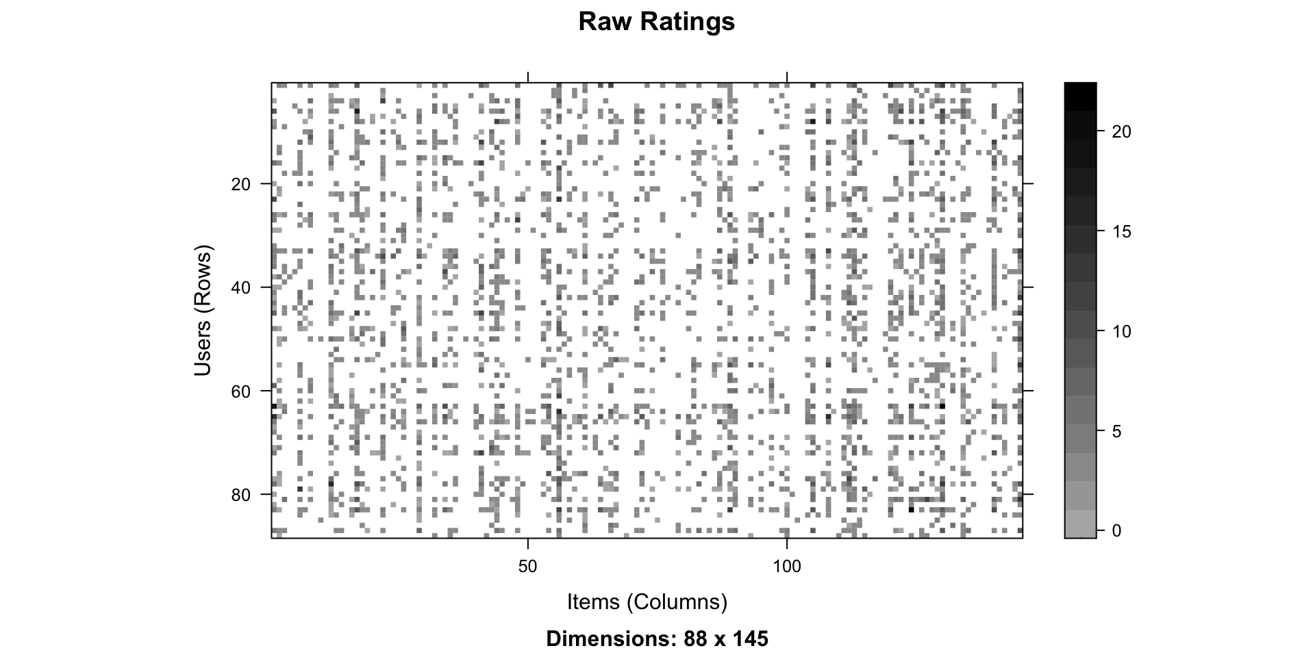
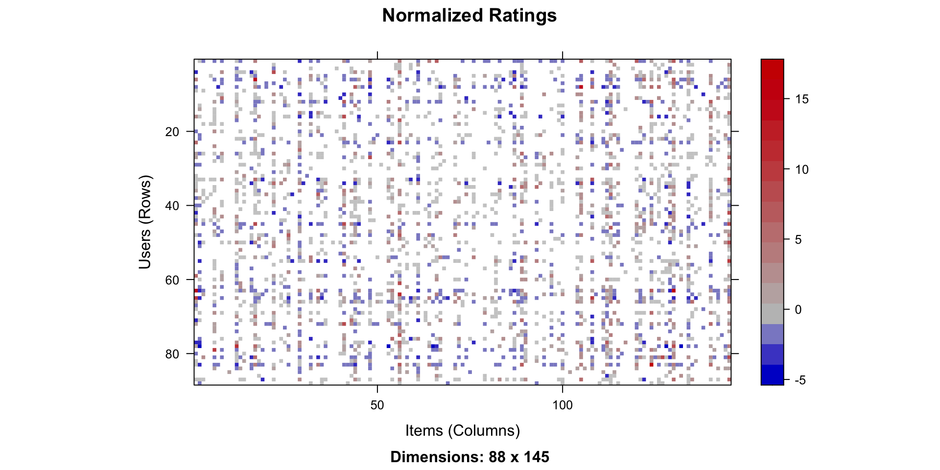
The dots below represent data for which there is no performance data. These cells need to be estimated by the algorithm
set.seed(2022)
r <- as(df8,"realRatingMatrix")
getRatingMatrix(r)[1:15,1:15]
## 15 x 15 sparse Matrix of class "dgCMatrix"
## [[ suppressing 15 column names 'A Mishra', 'A Nortje', 'A Zampa' ... ]]
The data frame of the batsman vs bowlers from the period 2020 -2022 is read as a dataframe. To remove rows with very low number of ratings(timesOut, SR, Fours, Sixes etc), the rows are filtered so that there are at least more 10 values in the row. For the player estimation the dataframe is converted into a wide-format as a matrix (m x n) of batsman x bowler with each of the columns of the dataframe i.e. timesOut, SR, fours or sixes. These different matrices can be considered as a rating matrix for estimation.
A similar approach is taken for estimating bowler performance. Here a wide form matrix (m x n) of bowler x batsman is created for each of the columns of deliveries, runsConceded, ER, wicketsTaken
5. Batsman’s times Out
The code below estimates the number of times the batsmen would lose his/her wicket to the bowler. As discussed in the algorithm above, the recommendation engine will make an initial estimate features for the bowler and an initial estimate for the parameter vector for the batsmen. Then using gradient descent the recommender engine will determine the feature and parameter values such that the over Mean Squared Error is minimum
From the plot for the different algorithms it can be seen that UBCF performs the best. However the AUC & ROC curves are not optimal and the AUC> 0.5
df3 <- select(df, batsman1,bowler1,timesOut)
df6 <- xtabs(timesOut ~ ., df3)
df7 <- as.data.frame.matrix(df6)
df8 <- data.matrix(df7)
df8[df8 == 0] <- NA
r <- as(df8,"realRatingMatrix")
# Filter only rows where the row count is > 10
r0=r[(rowCounts(r) > 10),]
getRatingMatrix(r0)[1:10,1:10]
## 10 x 10 sparse Matrix of class "dgCMatrix"
## [[ suppressing 10 column names 'A Mishra', 'A Nortje', 'A Zampa' ... ]]
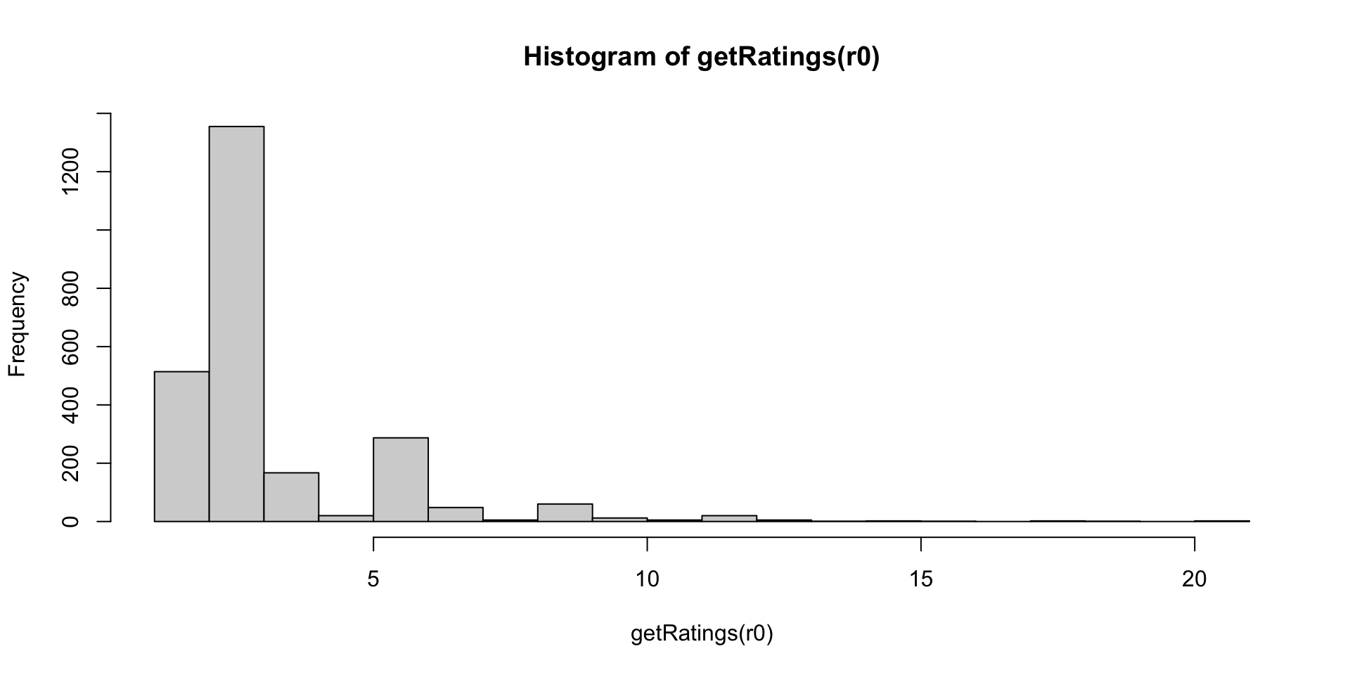
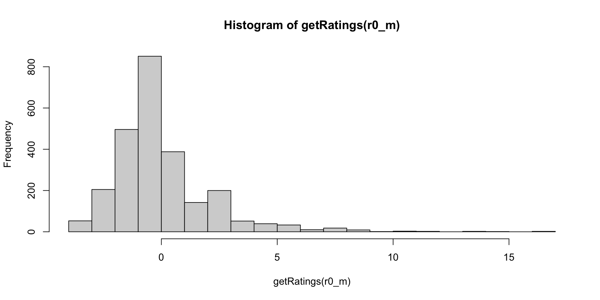
##    Min. 1st Qu.  Median    Mean 3rd Qu.    Max.
##   1.000   3.000   3.000   3.463   4.000  21.000
# Evaluate the different plotting methods
evalRecomMethods(r0[1:dim(r0)[1]],k1=5,given=7,goodRating1=median(getRatings(r0)))
#Evaluate the error
a=eval(r0[1:dim(r0)[1]],0.8,k1=5,given1=7,goodRating1=median(getRatings(r0)),"UBCF")
## Recommender of type 'UBCF' for 'realRatingMatrix'
## learned using 70 users.
## 18 x 145 rating matrix of class 'realRatingMatrix' with 1755 ratings.
##     RMSE      MSE      MAE
## 2.069027 4.280872 1.496388
b=round(as(a,"matrix")[1:10,1:10])
c <- as(b,"realRatingMatrix")
m=as(c,"data.frame")
names(m) =c("batsman","bowler","TimesOut")
6. Batsman’s Strike rate
This section deals with the Strike rate of batsmen versus bowlers and estimates the values for those where the data is incomplete using UBCF method.
Even here all the algorithms do not perform too efficiently. I did try out a few variations but could not lower the error (suggestions welcome!!)
## Recommender of type 'UBCF' for 'realRatingMatrix'
## learned using 105 users.
## 27 x 145 rating matrix of class 'realRatingMatrix' with 3220 ratings.
##       RMSE        MSE        MAE
##   77.71979 6040.36508   58.58484
b=round(as(a,"matrix")[1:10,1:10])
c <- as(b,"realRatingMatrix")
n=as(c,"data.frame")
names(n) =c("batsman","bowler","SR")
7. Batsman’s Sixes
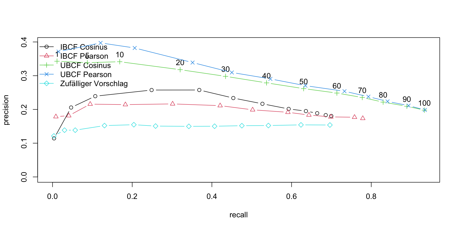
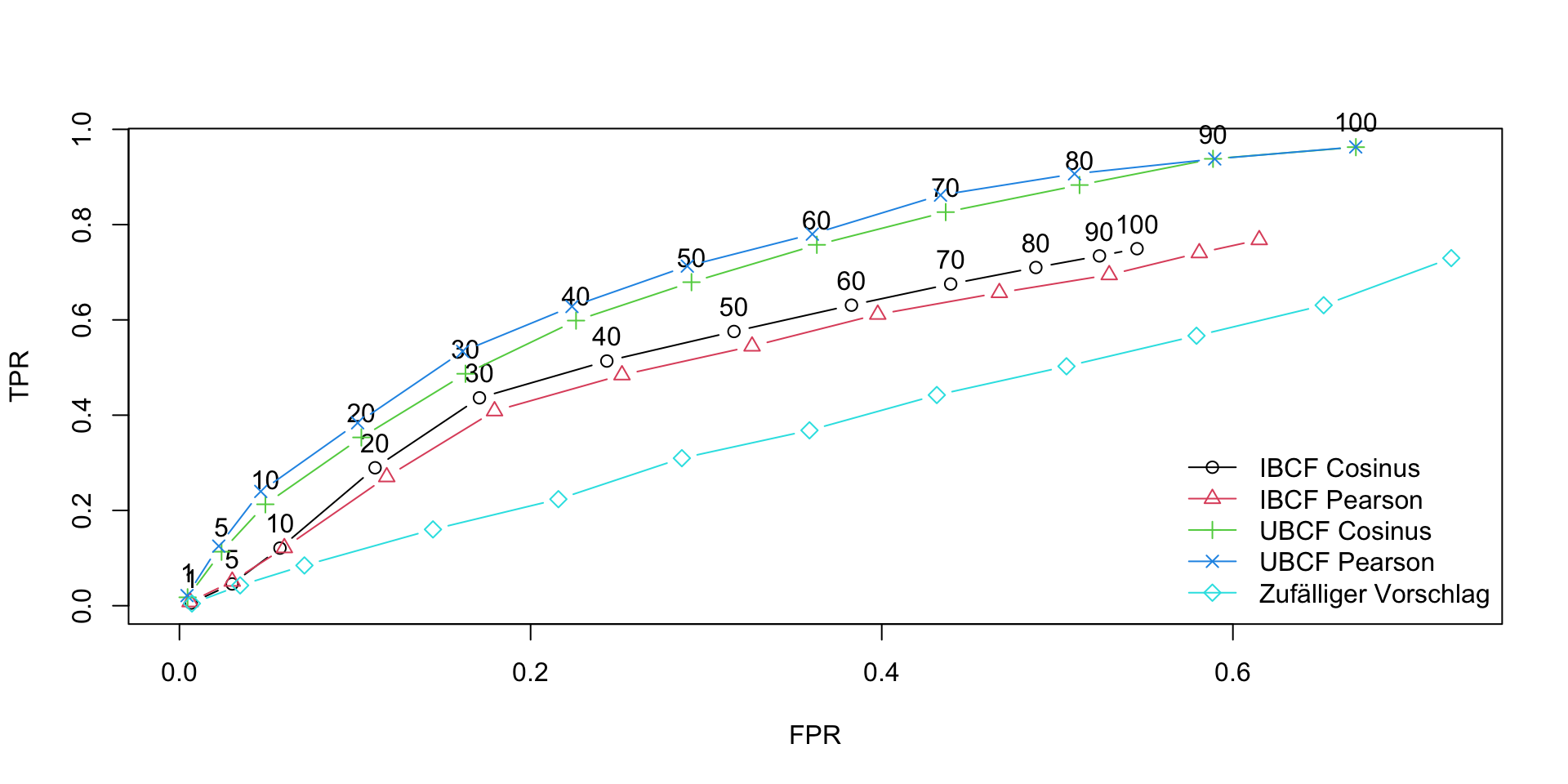
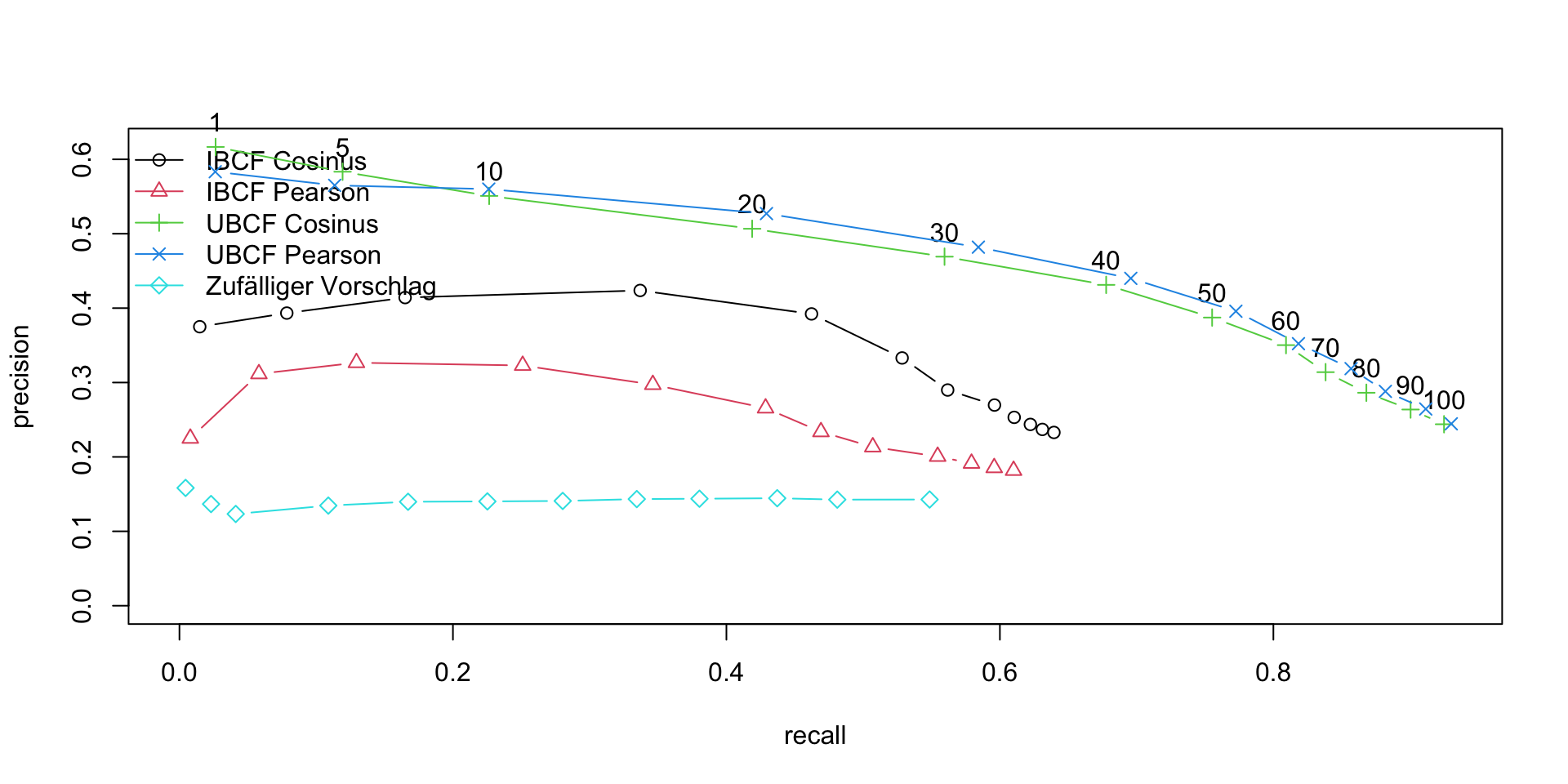
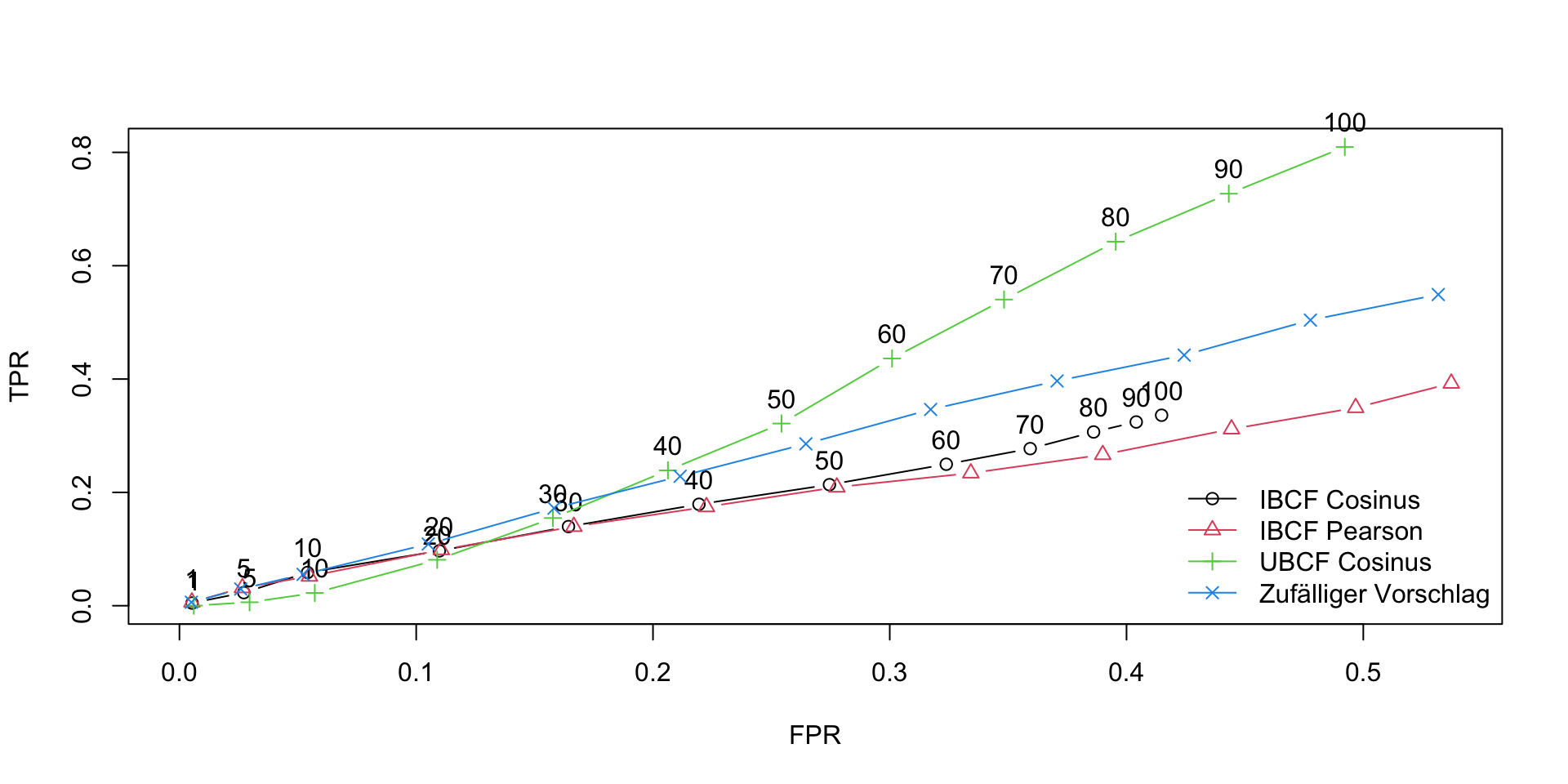
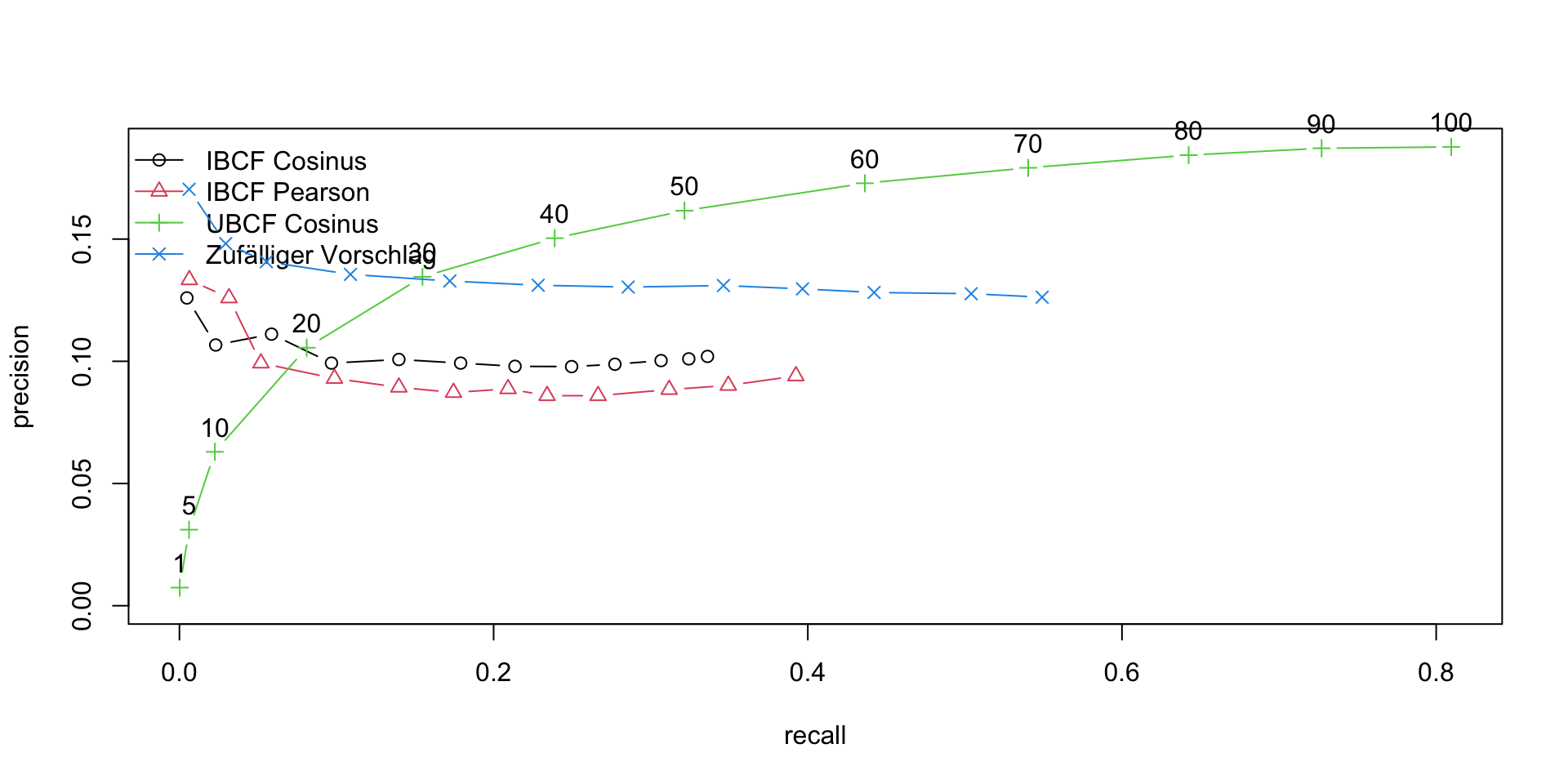
The snippet of code estimes the sixes of the batsman against bowlers. The ROC and AUC curve for UBCF looks a lot better here, as it significantly greater than 0.5
## Recommender of type 'UBCF' for 'realRatingMatrix'
## learned using 52 users.
## 14 x 145 rating matrix of class 'realRatingMatrix' with 1634 ratings.
##      RMSE       MSE       MAE
##  3.529922 12.460350  2.532122
b=round(as(a,"matrix")[1:10,1:10])
c <- as(b,"realRatingMatrix")
o=as(c,"data.frame")
names(o) =c("batsman","bowler","Sixes")
## Recommender of type 'UBCF' for 'realRatingMatrix'
## learned using 67 users.
## 17 x 145 rating matrix of class 'realRatingMatrix' with 2083 ratings.
##      RMSE       MSE       MAE
##  5.486661 30.103447  4.060990
b=round(as(a,"matrix")[1:10,1:10])
c <- as(b,"realRatingMatrix")
p=as(c,"data.frame")
names(p) =c("batsman","bowler","Fours")
9. Batsman’s Total Runs
The code below estimates the total runs that would have scored by the batsman against different bowlers
## Recommender of type 'UBCF' for 'realRatingMatrix'
## learned using 105 users.
## 27 x 145 rating matrix of class 'realRatingMatrix' with 3256 ratings.
##       RMSE        MSE        MAE
##   41.50985 1723.06788   29.52958
b=round(as(a,"matrix")[1:10,1:10])
c <- as(b,"realRatingMatrix")
q=as(c,"data.frame")
names(q) =c("batsman","bowler","TotalRuns")
10. Batsman’s Balls Faced
The snippet estimates the balls faced by batsmen versus bowlers
## Recommender of type 'UBCF' for 'realRatingMatrix'
## learned using 112 users.
## 28 x 145 rating matrix of class 'realRatingMatrix' with 3378 ratings.
##       RMSE        MSE        MAE
##   33.91251 1150.05835   23.39439
b=round(as(a,"matrix")[1:10,1:10])
c <- as(b,"realRatingMatrix")
r=as(c,"data.frame")
names(r) =c("batsman","bowler","BallsFaced")
11. Generate the Batsmen Performance Estimate
This code generates the estimated dataframe with known and ‘predicted’ values
##          batsman          bowler BallsFaced TotalRuns Fours Sixes  SR TimesOut
## 1 AB de Villiers        A Mishra         94       124     7     5 144        5
## 2 AB de Villiers        A Nortje         26        42     4     3 148        3
## 3 AB de Villiers         A Zampa         28        42     5     7 106        4
## 4 AB de Villiers Abhishek Sharma         22        28     0    10 136        5
## 5 AB de Villiers      AD Russell         70       135    14    12 207        4
## 6 AB de Villiers        AF Milne         31        45     6     6 130        3
12. Bowler analysis
Just like the batsman performance estimation we can consider the bowler’s performances also for estimation. Consider the following table
As in the batsman analysis, for every batsman a set of features like (“strong backfoot player”, “360 degree player”,“Power hitter”) can be estimated with a set of initial values. Also every bowler will have an associated parameter vector θθ. Different bowlers will have performance data for different set of batsmen. Based on the initial estimate of the features and the parameters, gradient descent can be used to minimize actual values {for e.g. wicketsTaken(ratings)}.
load("recom_data/bowlerVsBatsman20_22.rdata")
12a. Bowler dataframe
Inspecting the bowler dataframe
head(df2)
##    bowler1        batsman1 balls runsConceded       ER wicketTaken
## 1 A Mishra        A Badoni     0            0 0.000000           0
## 2 A Mishra       A Manohar     0            0 0.000000           0
## 3 A Mishra        A Nortje     0            0 0.000000           0
## 4 A Mishra  AB de Villiers    63           61 5.809524           0
## 5 A Mishra     Abdul Samad     0            0 0.000000           0
## 6 A Mishra Abhishek Sharma     2            3 9.000000           0
## Recommender of type 'UBCF' for 'realRatingMatrix'
## learned using 96 users.
## 24 x 195 rating matrix of class 'realRatingMatrix' with 3954 ratings.
##      RMSE       MSE       MAE
##  30.72284 943.89294  19.89204
b=round(as(a,"matrix")[1:10,1:10])
c <- as(b,"realRatingMatrix")
s=as(c,"data.frame")
names(s) =c("bowler","batsman","BallsBowled")
14. Runs conceded by bowler
This section estimates the runs conceded by the bowler. The UBCF Cosinus algorithm performs the best with TPR increasing fastewr than FPR
## Recommender of type 'UBCF' for 'realRatingMatrix'
## learned using 95 users.
## 24 x 195 rating matrix of class 'realRatingMatrix' with 3820 ratings.
##       RMSE        MSE        MAE
##   43.16674 1863.36749   30.32709
b=round(as(a,"matrix")[1:10,1:10])
c <- as(b,"realRatingMatrix")
t=as(c,"data.frame")
names(t) =c("bowler","batsman","RunsConceded")
15. Economy Rate of the bowler
This section computes the economy rate of the bowler. The performance is not all that good
## Recommender of type 'UBCF' for 'realRatingMatrix'
## learned using 95 users.
## 24 x 195 rating matrix of class 'realRatingMatrix' with 3839 ratings.
##      RMSE       MSE       MAE
##  4.380680 19.190356  3.316556
b=round(as(a,"matrix")[1:10,1:10])
c <- as(b,"realRatingMatrix")
u=as(c,"data.frame")
names(u) =c("bowler","batsman","EconomyRate")
16. Wickets Taken by bowler
The code below computes the wickets taken by the bowler versus different batsmen
## Recommender of type 'UBCF' for 'realRatingMatrix'
## learned using 64 users.
## 16 x 195 rating matrix of class 'realRatingMatrix' with 1908 ratings.
##     RMSE      MSE      MAE
## 2.672677 7.143203 1.956934
b=round(as(a,"matrix")[1:10,1:10])
c <- as(b,"realRatingMatrix")
v=as(c,"data.frame")
names(v) =c("bowler","batsman","WicketTaken")
17. Generate the Bowler Performance estmiate
The entire dataframe is regenerated with known and ‘predicted’ values
##     bowler         batsman BallsBowled RunsConceded EconomyRate WicketTaken
## 1 A Mishra  AB de Villiers         102          144           8           4
## 2 A Mishra     Abdul Samad          13           20           7           4
## 3 A Mishra Abhishek Sharma          14           26           8           2
## 4 A Mishra      AD Russell          47           85           9           3
## 5 A Mishra        AJ Finch          45           61          11           4
## 6 A Mishra          AJ Tye          14           20           5           4
18. Conclusion
This post showed an approach for performing the Batsmen Performance Estimate & Bowler Performance Estimate. The performance of the recommender engine could have been better. In any case, I think this approach will work for player estimation provided the recommender algorithm is able to achieve a high degree of accuracy. This will be a good way to estimate as the algorithm will be able to determine features and nuances of batsmen and bowlers which cannot be captured by data.
Where a calculator on the ENIAC is equipped with 18,000 vacuum tubes and weighs 30 tons, computers in the future may have only 1,000 vacuum tubes and perhaps weigh 1.5 tons.—POPULAR MECHANICS, 1949
Introduction: Ray Kurzweil in his non-fiction book “The Singularity is near – When humans transcend biology” predicts that by the year 2045 the Singularity will allow humans to transcend our ‘frail biological bodies’ and our ‘petty, derivative and circumscribed brains’ . Specifically the book claims “that there will be a ‘technological singularity’ in the year 2045, a point where progress is so rapid it outstrips humans’ ability to comprehend it. Irreversibly transformed, people will augment their minds and bodies with genetic alterations, nanotechnology, and artificial intelligence”.
He believes that advances in robotics, AI, nanotechnology and genetics will grow exponentially and will lead us into a future realm of intelligence that will far exceed biological intelligence. This explosion will be the result of ‘accelerating returns from significant advances in technology”
Futurescape
Here is a look at some of the more fascinating key trends in technology. You can decide whether we are heading to Singularity or not.
Autonomous Vehicles (AVs): Self driving cars have moved from the realm of science fiction to reality in recent times. Google’s autonomous cars has already driven around half a million miles. All the major car manufacturers of the world from BMW, Mercedes, Toyota, Nissan, Ford or GM are all coming with their own versions of autonomous cars. These cars are equipped with Adaptive Cruise Control and Collision Avoidance technologies and are already taking away control drivers. Moreover AVs alert drivers, if their attention strays from the road ahead, for too long. Autonomous Vehicles work with the help of Vehicular Communication Technology.
Vehicular Communication along with the Intelligent Transport Systems (ITS) achieves safety by enabling communication between vehicles, people and roads. Vehicle-to-vehicle communications are the fundamental building block of autonomous, self-driving cars. It enables the exchange of data between vehicles and allows automobiles to “see” and adapt to driving obstacles more completely, preventing accidents besides resulting in more efficient driving.
Smart Assistants: From the defeat of Kasparov in chess by IBM’s Deep Blue in 1997, and then subsequently to the resounding victory of IBM’s Watson in Jeopardy, capable of understanding natural human language, to the more prevalent Apple’s intelligent assistant Siri, Artificially Intelligent (AI) systems have come a long way. The newest trend in this area is Smart Assistants. Robots are currently analyzing documents, filling prescriptions, and handling other tasks that were once exclusively done by humans. Smart Assistants are already taking over the tasks of BPO operators, paralegals, store clerks, baby sitters. Robots, in many ways, are not only smarter than humans, but also do not get easily bored,
Intelligent homes and intelligent offices. Rapid advances in technology will be closer to the home both literally and figuratively. The future home will have the ability to detect the presence of people, pets, smoke and changes to humidity, moisture, lighting, temperature. Smart devices will monitor the environment and take appropriate steps to save energy, improve safety and enhance security of homes. Devices will start learning your habits and enhance your comfort and convenience. Everything from thermostats, fire detectors, washing machines, refrigerators will be equipped electronics that will be capable of adapting to the environment. All gadgets at home will be accessible through laptops, tablets or smartphones from anywhere. We will be able to monitor all aspects of our intelligent home from anywhere.
Smart devices will also make major inroads into offices leading to the birth of intelligent offices where the lighting, heating, cooling will be based on the presence of people in the offices. This will result in an enormous savings in energy. The advances in intelligent homes and intelligent offices will be in the greater context of the Smart Grid.
Swarms of drones: Contrary to the use of weaponized drones for unmanned aerial survey of enemy territory we will soon have commercial drones. Drone will start being used for civilian purposes. The most compelling aspect of drones these days is the fact that they can be easily manufactured in large quantities, are cheap and can perform complex tasks either singly or collectively. Remotely controlled drones can perform hundreds of civilian jobs, including traffic monitoring, aerial surveying, and oil pipeline inspections and monitoring of crop conditions. Drones are also being employed for conservation of wildlife. In the wilderness of Africa, drones are already helping in providing aerial footage of the landscape, tracking poachers and in also herding elephants. However, before drones become a common sight, it is necessary to ensure that appropriate laws are made for maintaining the safety and security of civilians. This is likely to happen in US in 2015, when the Federal Aviation Administration (FAA) will come up with rules to safely integrate drones into the American skies.
MOOC (Massive Online Open Course): The concept of MOOC, or the ‘Massive Open Online Course’ from top colleges, though just a few years old, is already taking the world by storm. Coursera, edX and Udacity are the top 3 MOOCs besides many others and offer a variety of courses on technology, philosophy, sociology, computer science etc. As more courses are available online, the requirements of having a uniform start and end date will diminish gradually. The availability of course lectures at all times and through all devices, namely the laptop, tablet or smartphone, will result in large scale adoption by students of all ages.
Contrary to regimented classes MOOCs now allow students to take classes at their own pace. It is likely that some students will breeze through an entire semester worth of classes in a few weeks. It is also likely that a few students will graduate in 4 years with more than a couple of degrees. MOOCs are a natural development considering that the world is going to be more knowledge driven where there will be the need for experts with a diverse set of in-depth skills. Here is an interesting article in WSJ “What College will be like in 2023”
3D Printing: This is another technology that is bound to become ubiquitous in our future. 3D printers will revolutionize manufacturing in ways we could never imagine. A 3-D printer is similar to a hot-glue gun attached to a robotic arm. A 3-D printer creates an object by stacking one layer of material, typically plastic or metal, on top of another. 3D printers have been used for making everything from prosthetic limbs, phone cases, lamps all the way to a NASA funded 3D pizza. Here is a great article in New York Times “Dinner is Printed” It is likely that a 3D printer would be indispensable to our future homes much like the refrigerator and microwave.
Artificial sense organs: A recent news items in Science 2.0 “The Future touch sensitive prosthetic limbs” discusses the invention of a prosthetic limb that can actually provide the sense of touch by stimulating the regions of the brain that deal with the sense of touch. The researchers identified the neural activity that occurs when grasping or feeling an object and successfully induced these patterns in the brain. Two parallel efforts are underway to understand how the human brain works. They are “The Human Brain Project” which has 130 members of the European Union and Obama’s BRAIN project. Both these projects attempt to ‘to give us a deeper and more meaningful understanding of how the human brain operates”. Possibilities as in the movies ‘Avatar’ or ‘Terminator’ may not be far away.
The Others: Besides the above, technologies like Big Data, Cloud Computing, Semantic Web, Internet of Things and Smart Grid will also be swamp us in the future and much has already been said about it.
Conclusion: The above sets of technologies represent seismic shifts and are bound to explode in our future in a million ways.
Given the advances in bionic limbs, Machine Intelligent AI systems, MOOCs, Autonomous Vehicles are we on target for the Singularity?
Pete Mettle felt drowsy. He had been working for days on his new inference algorithm. Pete had been in the field of Artificial Intelligence (AI) for close to 3 decades and had established himself as the father of “semantics”. He was particularly renowned for his 3 principles of Artificial Intelligence. He had postulated the Principles of Learning as
The Principle of Knowledge Acquisition: This principle laid out the guidelines for knowledge acquisition by an algorithm. It clearly laid out the rules of what was knowledge and what was not. It could clearly delineate between the wheat and chaff from any textbook or research article.
The Principle of Knowledge Assimilation: This law gave the process for organizing the acquired knowledge in facts, rules and underlying principles. Knowledge assimilation involved storing the individual rules, the relation between the rules and provided the basis for drawing conclusions from them
The Principle of Knowledge Application: This principle according to Pete was the most important. It showed how all knowledge acquired and assimilated could be used to draw inferences andconclusions. In fact it also showed how knowledge could be extrapolated to make safe conclusions.
Zengine The above 3 principles of Pete were hailed as a major landmark in AI. Pete started to work on an inference engine known as “Zengine” based on his above 3 principles. Pete was almost finished fine tuning his algorithm. Pete wanted to test his Zengine on the World Wide Web. The World Wide Web had grown into gigantic proportions. A report in May 2025 issue of Wall Street Journal mentioned that the total data that was held in the internet had crossed 400 zettabytes and that the daily data stored on the web was close to 20 terabytes. It was a well known fact that there an enormous amount of information on the web on a wide variety of topics. Wikis, blogs, articles, ideas, social networks and so on there was a lot of information on almost every conceivable topic under the sun.
Pete was given special permission by the governments of the world to run his Zengine on the internet. It was Pete’s theory that it would take the Zengine close to at least a year to process the information on the web and make any reasonable inferences from them. Accompanied by world wide publicity Zengine started its work of trying to assimilate the information on the World Wide Web. The Zengine was programmed to periodically give a status update of its progress to Pete.
A few months passed. Zengine kept giving updates on the number of sites, periodicals, blogs it had condensed into its knowledge database. After about 10 months Pete received a mail. It read “Markets will crash on March 2026. Petrol prices will sky rocket – Zengine. Pete was surprised at the forecast. So he invoked the API to check on what basis the claim had been made. To his surprise and amazement he found that a lot events happening in the world had been used to make that claim which clearly seemed to point in that direction. A couple of months down the line there was another terse statement “Rebellion very likely in Mogadishu in Dec 2027″. – Zengine.The Zengine also came with corollaries to Fermat’s last theorem. It was becoming clear to Pete and everybody that the Zengine was indeed becoming smarter by the day..It became apparent to everybody when Zengine would become more powerful than human beings.
Celestial events: Around this time peculiar events were observed all over the world. There were a lot of celestial events that were happening. Phenomenon like the aurora borealis became common place. On Dec 12, 2026 there was an unusual amount of electrical activity in the sky. Everywhere there were streaks of lightning. By evening time slivers of lightning hit the earth in several parts of the world. In fact if anybody had viewed the earth from outer space then it would have a resembled a “nebula sphere” with lightning streaks racing towards the earth in all directions. This seemed to happen for many days. Simultaneously the Zengine was getting more and more powerful. In fact it had learnt to spawn of multiple processes to get information and return to it.
Time-space discontinuity: People everywhere were petrified of this strange phenomenon. On the one hand there was the fear of the takeover of the web by the Zengine and on the other was this increased celestial activity. Finally on the morning of Jan 2028 there was a powerful crack followed by a sonic boom and everywhere people had a moment of discontinuity. In the briefest of moments there was a natural time-space discontinuity and mankind had progressed to the next stage in evolution.
The unconscious, sub conscious and the conscious all became a single faculty of super consciousness. It has always been known from the time of Plato that man knows everything there is to know. According to Platonic doctrine of Recollection, human beings are born with a soul possessing all knowledge, and learning is just discovering or recollecting what the soul already knows. Similarly according to Hindu philosophy, behind the individual consciousness of the Atman, is the reality known as the Brahman which is universal consciousness attained in a deep state of mysticism through self-inquiry.
However this evolution by some strange quirk of coincidence seemed to coincide with the development of the world’s first truly learning machine. In this super conscious state a learning machine was not something to be feared but something which could be used to benefit mankind. Just like cranes can lift and earthmovers perform tasks that are beyond our physical capacity so also a learning machine was a useful invention that could be used to harness the knowledge from mankind’s storehouse – the World Wide Web.


 scales the dot product so that the dot product values are not overly large


 and
and  are the weight matrices, and
  and
and  are the biases
  x
x  and
and x
x  and
and  is the activation function which can be ReLU, GELU or SwiGLU

 ,
,  ,
,  . By multiplyting these matrices with the input vectors we get Q,K and V vectors. The attention is computed as


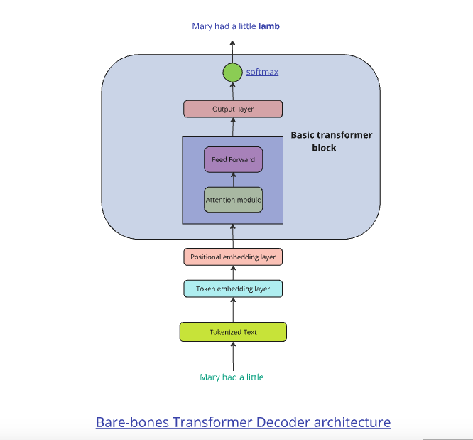
 ,
, 


 = 64
= 64
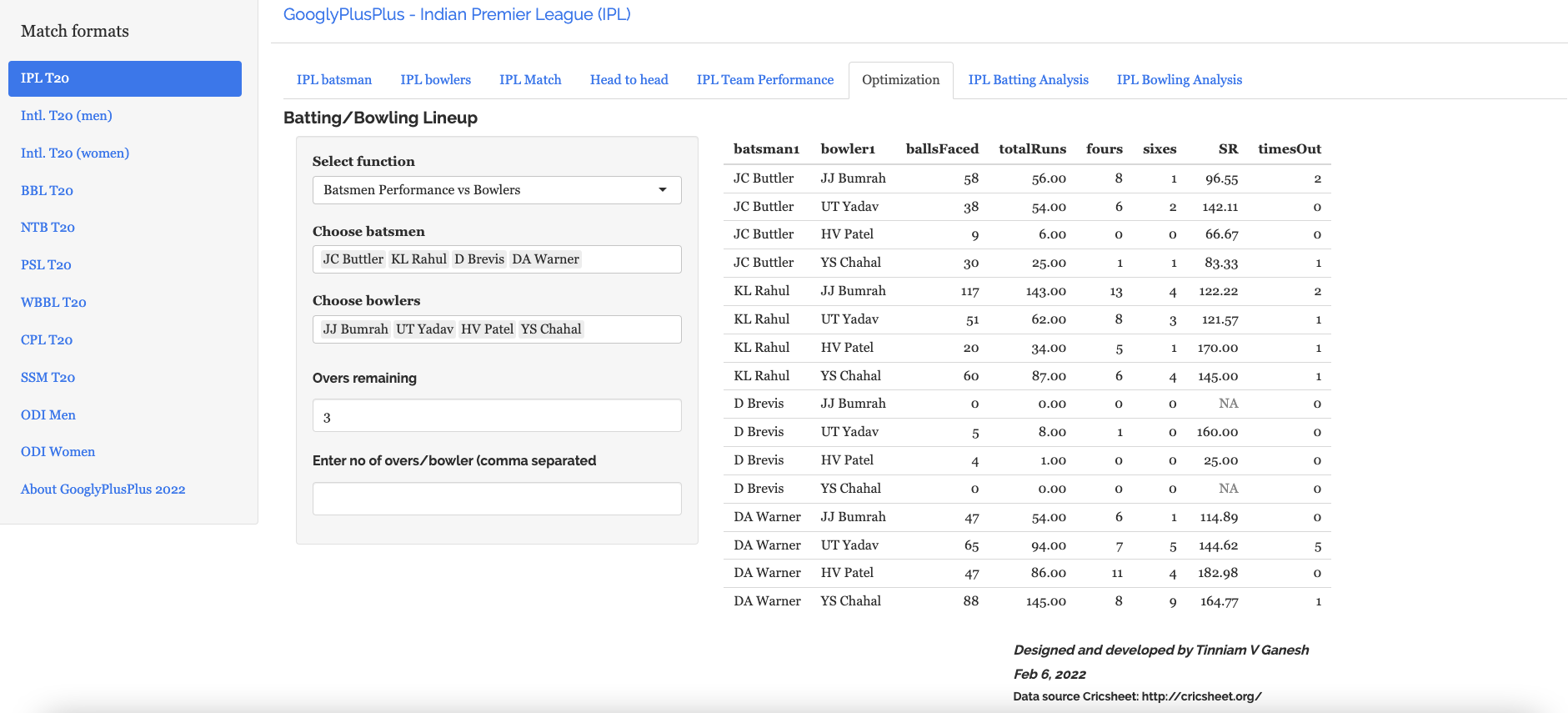
 ,
,  and
and  for the 3 bowlers which identify the characteristics of these bowlers (“fast”, “lateral drift through the air”, “movement off the pitch”). Let each batsman be identified by parameter vectors
  ,
,  and so on
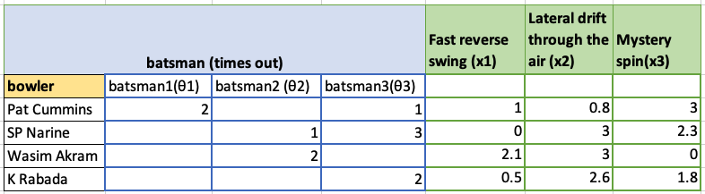
 and the feature vector xx we can formulate this as an optimization problem which tries to minimize the error for
  This can work very well as the algorithm can determine features which cannot be captured. So for e.g. some particular bowler may have very impressive figures. This could be due to some aspect of the bowling which cannot be captured by the data for e.g. let’s say the bowler uses the ‘scrambled seam’ when he is most effective, with a slightly different arc to the flight. Though the algorithm cannot identify the feature as we know it, but the ML algorithm should pick up intricacies which cannot be captured in data.
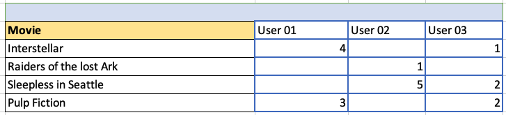
 ,
,  }= 1/2
 and the set of features be
  to small random values
 , i= 1,2,..,
 :=
:=  (
(  )
) –
– 
 :=
:=