“What does the world outside your head really ‘look’ like? Not only is there no color, there’s also no sound: the compression and expansion of air is picked up by the ears, and turned into electrical signals. The brain then presents these signals to us as mellifluous tones and swishes and clatters and jangles. Reality is also odorless: there’s no such thing as smell outside our brains. Molecules floating through the air bind to receptors in our nose and are interpreted as different smells by our brain. The real world is not full of rich sensory events; instead, our brains light up the world with their own sensuality.”
The Brain: The Story of You” by David Eagleman
“The world is Maya, illusory. The ultimate reality, the Brahman, is all-pervading and all-permeating, which is colourless, odourless, tasteless, nameless and formless“
Bhagavad Gita
1. Introduction
This post is a follow-up post to my earlier post Deep Learning from first principles in Python, R and Octave-Part 1. In the first part, I implemented Logistic Regression, in vectorized Python,R and Octave, with a wannabe Neural Network (a Neural Network with no hidden layers). In this second part, I implement a regular, but somewhat primitive Neural Network (a Neural Network with just 1 hidden layer). The 2nd part implements classification of manually created datasets, where the different clusters of the 2 classes are not linearly separable.
Neural Network perform really well in learning all sorts of non-linear boundaries between classes. Initially logistic regression is used perform the classification and the decision boundary is plotted. Vanilla logistic regression performs quite poorly. Using SVMs with a radial basis kernel would have performed much better in creating non-linear boundaries. To see R and Python implementations of SVMs take a look at my post Practical Machine Learning with R and Python – Part 4.
 Checkout my book ‘Deep Learning from first principles: Second Edition – In vectorized Python, R and Octave’. My book starts with the implementation of a simple 2-layer Neural Network and works its way to a generic L-Layer Deep Learning Network, with all the bells and whistles. The derivations have been discussed in detail. The code has been extensively commented and included in its entirety in the Appendix sections. My book is available on Amazon as paperback ($18.99) and in kindle version($9.99/Rs449).
You can download the PDF version of this book from Github at https://github.com/tvganesh/DeepLearningBook-2ndEd
You may also like my companion book “Practical Machine Learning with R and Python:Second Edition- Machine Learning in stereo” available in Amazon in paperback($10.99) and Kindle($7.99/Rs449) versions. This book is ideal for a quick reference of the various ML functions and associated measurements in both R and Python which are essential to delve deep into Deep Learning.
Take a look at my video presentation which discusses the below derivation step-by- step Elements of Neural Networks and Deep Learning – Part 3
You can clone and fork this R Markdown file along with the vectorized implementations of the 3 layer Neural Network for Python, R and Octave from Github DeepLearning-Part2
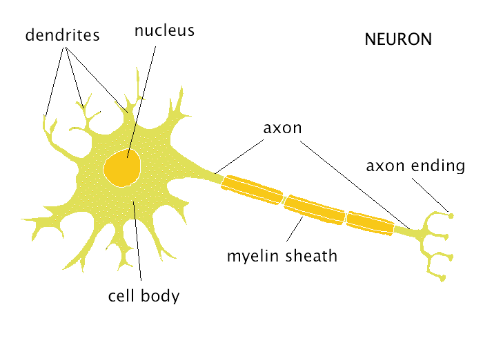
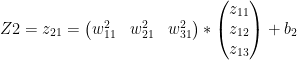
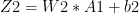
2. The 3 layer Neural Network
A simple representation of a 3 layer Neural Network (NN) with 1 hidden layer is shown below.

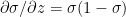
In the above Neural Network, there are 2 input features at the input layer, 3 hidden units at the hidden layer and 1 output layer as it deals with binary classification. The activation unit at the hidden layer can be a tanh, sigmoid, relu etc. At the output layer the activation is a sigmoid to handle binary classification
# Superscript indicates layer 1

Also


# Superscript indicates layer 2

Hence
And


Similarly
and

These equations can be written as

I) Some important results (a memory refresher!)

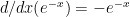
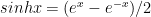
Using (a) we can shown that 
Now 

Since 
Using the values of the derivatives of sinhx and coshx from (b) above we get
Since


II) Derivatives
Since 


III) Back propagation
Using the derivatives from II) we can derive the following results using Chain Rule


IV) Gradient Descent
The key computations in the backward cycle are


The weights and biases (W1,b1,W2,b2) are updated for each iteration thus minimizing the loss/cost.
These derivations can be represented pictorially using the computation graph (from the book Deep Learning by Ian Goodfellow, Joshua Bengio and Aaron Courville)

3. Manually create a data set that is not lineary separable
Initially I create a dataset with 2 classes which has around 9 clusters that cannot be separated by linear boundaries. Note: This data set is saved as data.csv and is used for the R and Octave Neural networks to see how they perform on the same dataset.
import numpy as np
import matplotlib.pyplot as plt
import matplotlib.colors
import sklearn.linear_model

from sklearn.model_selection import train_test_split
from sklearn.datasets import make_classification, make_blobs
from matplotlib.colors import ListedColormap
import sklearn
import sklearn.datasets


colors=['black','gold']
cmap = matplotlib.colors.ListedColormap(colors)
X, y = make_blobs(n_samples = 400, n_features = 2, centers = 7,
                       cluster_std = 1.3, random_state = 4)
#Create 2 classes
y=y.reshape(400,1)
y = y % 2
#Plot the figure
plt.figure()
plt.title('Non-linearly separable classes')
plt.scatter(X[:,0], X[:,1], c=y,
           marker= 'o', s=50,cmap=cmap)
plt.savefig('fig1.png', bbox_inches='tight')
4. Logistic Regression
On the above created dataset, classification with logistic regression is performed, and the decision boundary is plotted. It can be seen that logistic regression performs quite poorly
import numpy as np
import matplotlib.pyplot as plt
import matplotlib.colors
import sklearn.linear_model

from sklearn.model_selection import train_test_split
from sklearn.datasets import make_classification, make_blobs
from matplotlib.colors import ListedColormap
import sklearn
import sklearn.datasets

#from DLfunctions import plot_decision_boundary
execfile("./DLfunctions.py") # Since import does not work in Rmd!!!

colors=['black','gold']
cmap = matplotlib.colors.ListedColormap(colors)
X, y = make_blobs(n_samples = 400, n_features = 2, centers = 7,
                       cluster_std = 1.3, random_state = 4)
#Create 2 classes
y=y.reshape(400,1)
y = y % 2

# Train the logistic regression classifier
clf = sklearn.linear_model.LogisticRegressionCV();
clf.fit(X, y);

# Plot the decision boundary for logistic regression
plot_decision_boundary_n(lambda x: clf.predict(x), X.T, y.T,"fig2.png")

5. The 3 layer Neural Network in Python (vectorized)
The vectorized implementation is included below. Note that in the case of Python a learning rate of 0.5 and 3 hidden units performs very well.
## Random data set with 9 clusters
import numpy as np
import matplotlib
import matplotlib.pyplot as plt
import sklearn.linear_model
import pandas as pd

from sklearn.datasets import make_classification, make_blobs
execfile("./DLfunctions.py") # Since import does not work in Rmd!!!

X1, Y1 = make_blobs(n_samples = 400, n_features = 2, centers = 9,
                       cluster_std = 1.3, random_state = 4)
#Create 2 classes
Y1=Y1.reshape(400,1)
Y1 = Y1 % 2
X2=X1.T
Y2=Y1.T

#Perform gradient descent
parameters,costs = computeNN(X2, Y2, numHidden = 4, learningRate=0.5, numIterations = 10000)
plot_decision_boundary(lambda x: predict(parameters, x.T), X2, Y2,str(4),str(0.5),"fig3.png")
## Cost after iteration 0: 0.692669
## Cost after iteration 1000: 0.246650
## Cost after iteration 2000: 0.227801
## Cost after iteration 3000: 0.226809
## Cost after iteration 4000: 0.226518
## Cost after iteration 5000: 0.226331
## Cost after iteration 6000: 0.226194
## Cost after iteration 7000: 0.226085
## Cost after iteration 8000: 0.225994
## Cost after iteration 9000: 0.225915
6. The 3 layer Neural Network in R (vectorized)
For this the dataset created by Python is saved to see how R performs on the same dataset. The vectorized implementation of a Neural Network was just a little more interesting as R does not have a similar package like ‘numpy’. While numpy handles broadcasting implicitly, in R I had to use the ‘sweep’ command to broadcast. The implementaion is included below. Note that since the initialization with random weights is slightly different, R performs best with a learning rate of 0.1 and with 6 hidden units
source("DLfunctions2_1.R")z <- as.matrix(read.csv("data.csv",header=FALSE)) #
x <- z[,1:2]
y <- z[,3]
x1 <- t(x)
y1 <- t(y)
#Perform gradient descent
nn <-computeNN(x1, y1, 6, learningRate=0.1,numIterations=10000) # Good## [1] 0.7075341
## [1] 0.2606695
## [1] 0.2198039
## [1] 0.2091238
## [1] 0.211146
## [1] 0.2108461
## [1] 0.2105351
## [1] 0.210211
## [1] 0.2099104
## [1] 0.2096437
## [1] 0.209409plotDecisionBoundary(z,nn,6,0.1)

7. The 3 layer Neural Network in Octave (vectorized)
This uses the same dataset that was generated using Python code.
source("DL-function2.m")

data=csvread("data.csv");

X=data(:,1:2);

Y=data(:,3);

# Make sure that the model parameters are correct. Take the transpose of X & Y
#Perform gradient descent

[W1,b1,W2,b2,costs]= computeNN(X', Y',4, learningRate=0.5, numIterations = 10000);

8a. Performance for different learning rates (Python)
import numpy as np
import matplotlib
import matplotlib.pyplot as plt
import sklearn.linear_model
import pandas as pd

from sklearn.datasets import make_classification, make_blobs
execfile("./DLfunctions.py") # Since import does not work in Rmd!!!
# Create data
X1, Y1 = make_blobs(n_samples = 400, n_features = 2, centers = 9,
                       cluster_std = 1.3, random_state = 4)
#Create 2 classes
Y1=Y1.reshape(400,1)
Y1 = Y1 % 2
X2=X1.T
Y2=Y1.T
# Create a list of learning rates
learningRate=[0.5,1.2,3.0]
df=pd.DataFrame()
#Compute costs for each learning rate
for lr in learningRate:
   parameters,costs = computeNN(X2, Y2, numHidden = 4, learningRate=lr, numIterations = 10000)
   print(costs)
   df1=pd.DataFrame(costs)
   df=pd.concat([df,df1],axis=1)
#Set the iterations
iterations=[0,1000,2000,3000,4000,5000,6000,7000,8000,9000]
#Create data frame
#Set index
df1=df.set_index([iterations])
df1.columns=[0.5,1.2,3.0]
fig=df1.plot()
fig=plt.title("Cost vs No of Iterations for different learning rates")
plt.savefig('fig4.png', bbox_inches='tight')

9a. Performance for different learning rates (R)
source("DLfunctions2_1.R")
# Read data
z <- as.matrix(read.csv("data.csv",header=FALSE)) #
x <- z[,1:2]
y <- z[,3]
x1 <- t(x)
y1 <- t(y)
#Loop through learning rates and compute costs
learningRate <-c(0.1,1.2,3.0)
df <- NULL
for(i in seq_along(learningRate)){
   nn <-  computeNN(x1, y1, 6, learningRate=learningRate[i],numIterations=10000)
   cost <- nn$costs
   df <- cbind(df,cost)

}
#Create dataframe
df <- data.frame(df)
iterations=seq(0,10000,by=1000)
df <- cbind(iterations,df)
names(df) <- c("iterations","0.5","1.2","3.0")
library(reshape2)
df1 <- melt(df,id="iterations") # Melt the data
#Plot
ggplot(df1) + geom_line(aes(x=iterations,y=value,colour=variable),size=1) +
xlab("Iterations") +
ylab('Cost') + ggtitle("Cost vs No iterations for different learning rates")

10a. Performance of the Neural Network for different learning rates (Octave)
source("DL-function2.m")

plotLRCostVsIterations()

print -djph figa.jpg


11. Turning the heat on the Neural Network
In this 2nd part I create a a central region of positives and and the outside region as negatives. The points are generated using the equation of a circle (x – a)^{2} + (y -b) ^{2} = R^{2} . How does the 3 layer Neural Network perform on this? Here’s a look! Note: The same dataset is also used for R and Octave Neural Network constructions
12. Manually creating a circular central region
import numpy as np
import matplotlib.pyplot as plt
import matplotlib.colors
import sklearn.linear_model

from sklearn.model_selection import train_test_split
from sklearn.datasets import make_classification, make_blobs
from matplotlib.colors import ListedColormap
import sklearn
import sklearn.datasets

colors=['black','gold']
cmap = matplotlib.colors.ListedColormap(colors)
x1=np.random.uniform(0,10,800).reshape(800,1)
x2=np.random.uniform(0,10,800).reshape(800,1)
X=np.append(x1,x2,axis=1)
X.shape
# Create (x-a)^2 + (y-b)^2 = R^2
# Create a subset of values where squared is <0,4. Perform ravel() to flatten this vector
a=(np.power(X[:,0]-5,2) + np.power(X[:,1]-5,2) <= 6).ravel()
Y=a.reshape(800,1)

cmap = matplotlib.colors.ListedColormap(colors)

plt.figure()
plt.title('Non-linearly separable classes')
plt.scatter(X[:,0], X[:,1], c=Y,
           marker= 'o', s=15,cmap=cmap)
plt.savefig('fig6.png', bbox_inches='tight')


 (1)
(1)

 then
then


 -(2)
-(2) -(a)
-(a) -(b)
-(b) -(c)
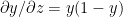
-(c) and
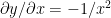
and  . In the case of regression it would be
  and
and  where dE is the Mean Squared Error function.
 -(d)
-(d)
 – (e)
– (e)
 (f)
(f) -(g)
-(g) – (h)
– (h)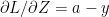
 -(i)
-(i) -(j)
-(j) and using (f) in (j)
 and
and 


 -(A)
-(A)


 for each weight
  . This is shown below

 -(B)
-(B)
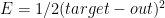
![\partial E _{total}/\partial out_{o1} = \partial /\partial _{out_{o1}}[1/2(target_{01}-out_{01})^{2}- 1/2(target_{02}-out_{02})^{2}]](https://s0.wp.com/latex.php?latex=%C2%A0%5Cpartial+E+_%7Btotal%7D%2F%5Cpartial+out_%7Bo1%7D+%3D+%5Cpartial+%2F%5Cpartial+_%7Bout_%7Bo1%7D%7D%5B1%2F2%28target_%7B01%7D-out_%7B01%7D%29%5E%7B2%7D-+1%2F2%28target_%7B02%7D-out_%7B02%7D%29%5E%7B2%7D%5D&bg=ffffff&fg=000000&s=0&c=20201002)

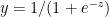
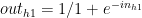
![\partial out_{o1}/\partial in_{o1} = \partial/\partial in_{o1} [1/(1+e^{-in_{o1}})]](https://s0.wp.com/latex.php?latex=%5Cpartial+out_%7Bo1%7D%2F%5Cpartial+in_%7Bo1%7D+%3D+%5Cpartial%2F%5Cpartial+in_%7Bo1%7D+%5B1%2F%281%2Be%5E%7B-in_%7Bo1%7D%7D%29%5D&bg=ffffff&fg=000000&s=0&c=20201002)
![\partial out_{o1}/\partial in_{o1} = \partial/\partial in_{o1} [1/(1+e^{-in_{o1}})] = out_{o1}(1-out_{o1})](https://s0.wp.com/latex.php?latex=%C2%A0%5Cpartial+out_%7Bo1%7D%2F%5Cpartial+in_%7Bo1%7D+%3D+%5Cpartial%2F%5Cpartial+in_%7Bo1%7D+%5B1%2F%281%2Be%5E%7B-in_%7Bo1%7D%7D%29%5D+%3D+out_%7Bo1%7D%281-out_%7Bo1%7D%29&bg=ffffff&fg=000000&s=0&c=20201002)
![\partial in_{o1}/\partial w_{5} = \partial/\partial w_{5} [w_{5}*out_{h1} + w_{6}*out_{h2}] = out_{h1}](https://s0.wp.com/latex.php?latex=%C2%A0%5Cpartial+in_%7Bo1%7D%2F%5Cpartial+w_%7B5%7D+%3D+%5Cpartial%2F%5Cpartial+w_%7B5%7D+%5Bw_%7B5%7D%2Aout_%7Bh1%7D+%2B+w_%7B6%7D%2Aout_%7Bh2%7D%5D+%3D+out_%7Bh1%7D&bg=ffffff&fg=000000&s=0&c=20201002)

 , we now perform gradient descent, by computing a new weight, assuming a learning rate

 we would get


 – (C)
– (C)
 -(D)
-(D)


 – (E)
– (E) – (F)
– (F)![\partial E_{total}/\partial w_{1} = -[(target_{o1}-out_{o1}) *out_{o1}(1-out_{o1})*w_{5} + (target_{o2}-out_{o2}) *out_{o2}(1-out_{o2})*w_{6}]*out_{h1}*(1-out_{h1})*i_{1}](https://s0.wp.com/latex.php?latex=%5Cpartial+E_%7Btotal%7D%2F%5Cpartial+w_%7B1%7D+%3D+-%5B%28target_%7Bo1%7D-out_%7Bo1%7D%29+%2Aout_%7Bo1%7D%281-out_%7Bo1%7D%29%2Aw_%7B5%7D+%2B+%28target_%7Bo2%7D-out_%7Bo2%7D%29+%2Aout_%7Bo2%7D%281-out_%7Bo2%7D%29%2Aw_%7B6%7D%5D%2Aout_%7Bh1%7D%2A%281-out_%7Bh1%7D%29%2Ai_%7B1%7D&bg=ffffff&fg=000000&s=0&c=20201002)
![\partial E_{total}/\partial w_{1} = -\sum_{i}[(target_{oi}-out_{oi}) *out_{oi}(1-out_{oi})*w_{j}]*out_{h1}*(1-out_{h1})*i_{1}](https://s0.wp.com/latex.php?latex=%5Cpartial+E_%7Btotal%7D%2F%5Cpartial+w_%7B1%7D+%3D+-%5Csum_%7Bi%7D%5B%28target_%7Boi%7D-out_%7Boi%7D%29+%2Aout_%7Boi%7D%281-out_%7Boi%7D%29%2Aw_%7Bj%7D%5D%2Aout_%7Bh1%7D%2A%281-out_%7Bh1%7D%29%2Ai_%7B1%7D&bg=ffffff&fg=000000&s=0&c=20201002)


![\partial E_{total}/\partial w_{k} = -\sum_{i}[(target_{oi}-out_{oi}) *out_{oi}(1-out_{oi})*w_{j}]*out_{hk}*(1-out_{hk})*i_{k}](https://s0.wp.com/latex.php?latex=%5Cpartial+E_%7Btotal%7D%2F%5Cpartial+w_%7Bk%7D+%3D+-%5Csum_%7Bi%7D%5B%28target_%7Boi%7D-out_%7Boi%7D%29+%2Aout_%7Boi%7D%281-out_%7Boi%7D%29%2Aw_%7Bj%7D%5D%2Aout_%7Bhk%7D%2A%281-out_%7Bhk%7D%29%2Ai_%7Bk%7D&bg=ffffff&fg=000000&s=0&c=20201002)