In this post, I compute each batsman’s or bowler’s Win Probability Contribution (WPC) in a T20 match. This metric captures by how much the player (batsman or bowler) changed/impacted the Win Probability of the T20 match. For this computation I use my machine learning models, I had created earlier, which predicts the ball-by-ball win probability as the T20 match progresses through the 2 innings of the match.
In the picture snippet below, you can see how the win probability changes ball-by-ball for each batsman for a T20 match between CSK vs LSG- 31 Mar 2022
In my previous posts I had created several Machine Learning models. In order to compute the player’s Win Probability contribution in this post, I have used the following ML models
The batsman’s or bowler’s win probability contribution changes ball-by=ball. The player’s contribution is calculated as the difference in win probability when the batsman faces the 1st ball in his innings and the last ball either when is out or the innings comes to an end. If the difference is +ve the the player has had a positive impact, and likewise for negative contribution. Similarly, for a bowler, it is the win probability when he/she comes into bowl till, the last delivery he/she bowls
Note: The Win Probability Contribution does not have any relation to the how much runs or at what strike rate the batsman scored the runs. Rather the model computes different win probability for each player, based on his/her embedding, the ball in the innings and six other feature vectors like runs, run rate, runsMomentum etc. These values change for every ball as seen in the table above. Also, this is not continuous. The 2 ML models determine the Win Probability for a specific player, ball and the context in the match.
This metric is similar to Win Probability Added (WPA) used in Sabermetrics for baseball. Here is the definition of WPA from Fangraphs “Win Probability Added (WPA) captures the change in Win Expectancy from one plate appearance to the next and credits or debits the player based on how much their action increased their team’s odds of winning.” This article in Fangraphs explains in detail how this computation is done.
In this post I have added 4 new function to my R package yorkr.
batsmanWinProbLR – batsman’s win probability contribution based on glmnet (Logistic Regression)
bowlerWinProbLR – bowler’s win probability contribution based on glmnet (Logistic Regression)
batsmanWinProbDL – batsman’s win probability contribution based on Deep Learning Model
bowlerWinProbDL – bowlerWinProbLR – bowler’s win probability contribution based on Deep Learning
Hence there are 4 additional features in GooglyPlusPlus based on the above 4 functions. In addition I have also updated
-winProbLR (overLap) function to include the names of batsman when they come to bat and when they get out or the innings comes to an end, based on Logistic Regression
-winProbDL(overLap) function to include the names of batsman when they come to bat and when they get out based on Deep Learning
Hence there are 6 new features in this version of GooglyPlusPlus.
Note: All these new 6 features are available for all 9 formats of T20 in GooglyPlusPlus namely
a) IPL b) BBL c) NTB d) PSL e) Intl, T20 (men) f) Intl. T20 (women) g) WBB h) CSL i) SSM
Check out the latest version of GooglyPlusPlus at gpp2023-2
Note: The data for GooglyPlusPlus comes from Cricsheet and the Shiny app is based on my R package yorkr
A) Chennai SuperKings vs Delhi Capitals – 04 Oct 2021
To understand Win Probability Contribution better let us look at Chennai Super Kings vs Delhi Capitals match on 04 Oct 2021
This was closely fought match with fortunes swinging wildly. If we take a look at the Worm wicket chart of this match
a) Worm Wicket chart – CSK vs DC – 04 Oct 2021
Delhi Capitals finally win the match
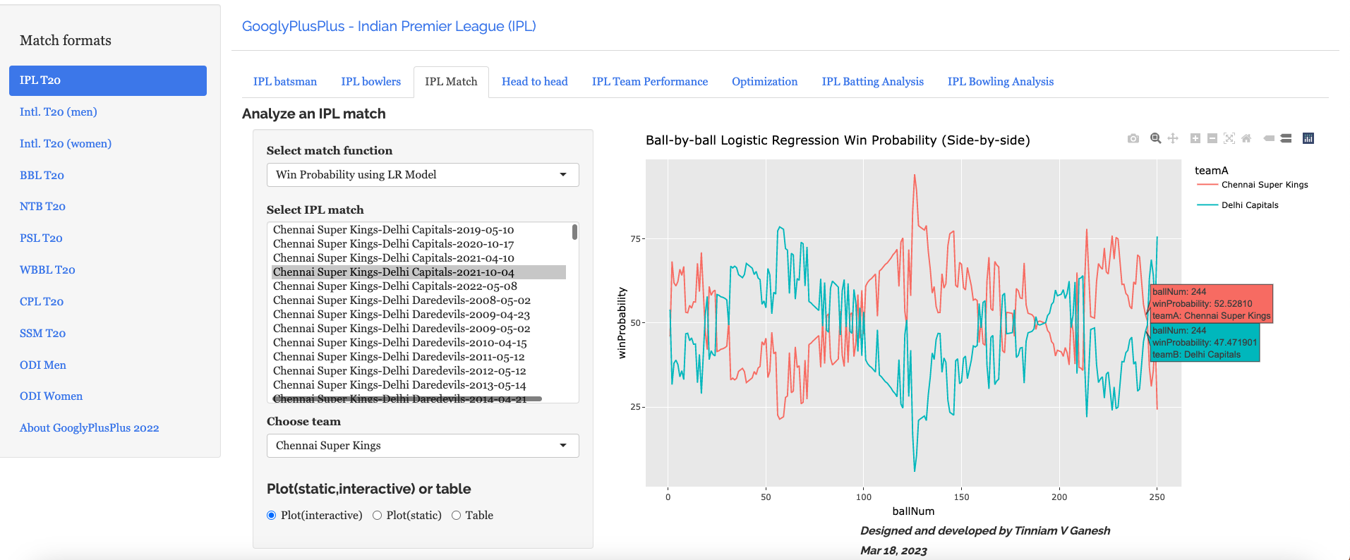
b) Win Probability Logistic Regression (side-by-side) – CSK vs DC – 4 Oct 2021
Plotting how win probability changes over the course of the match using Logistic Regression Model
In this match Delhi Capitals won. The batting scorecard of Delhi Capitals
c) Batting Scorecard of Delhi Capitals – CSK vs DC – 4 Oct 2021
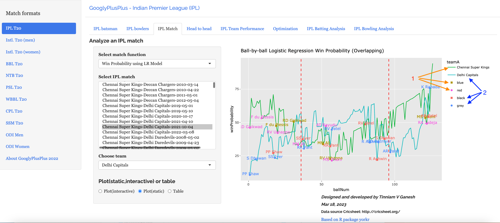
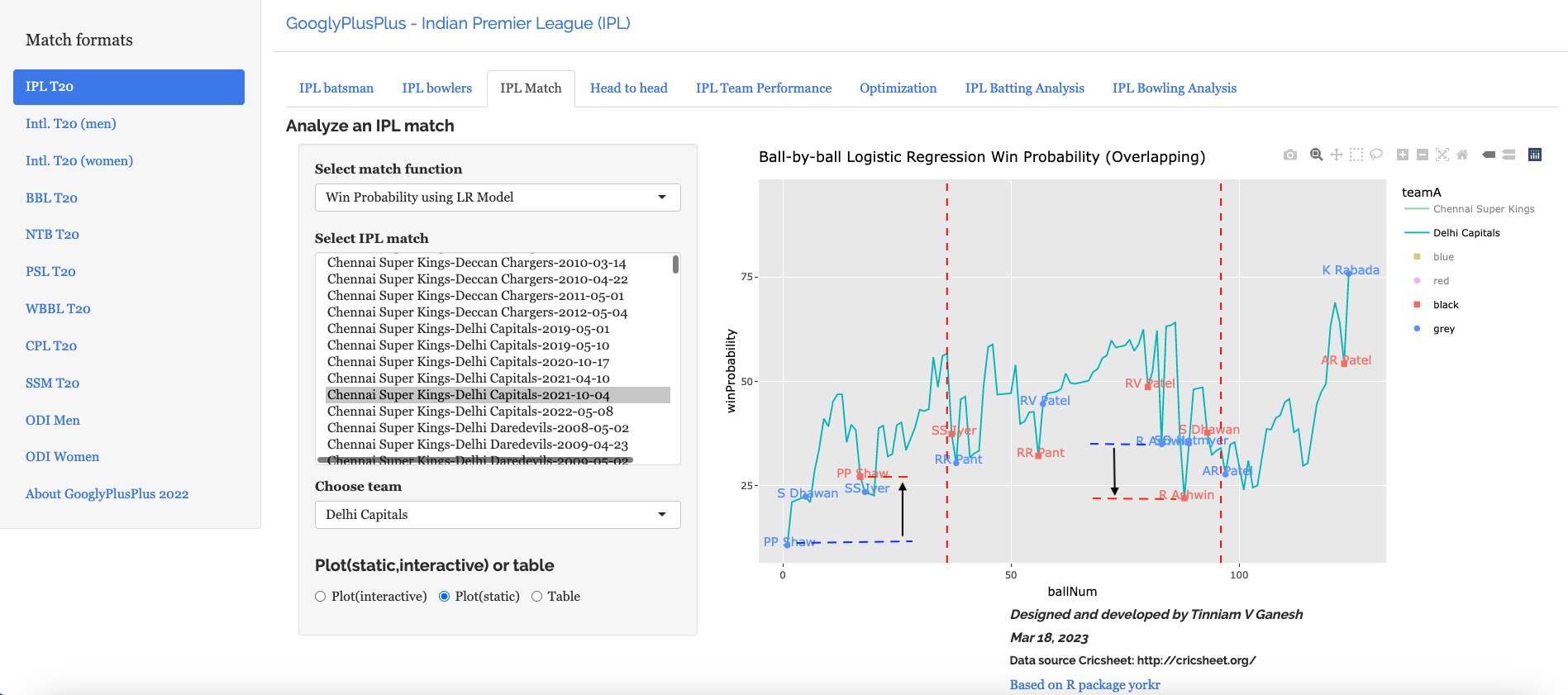
d) Win Probability Logistic Regression (Overlapping) – CSK vs DC – 4 Oct 2021
The Win Probability LR (overlapping) shows the probability function of both teams superimposed over one another. The plot includes when a batsman came into to play and when he got out. This is for both teams. This looks a little noisy, but there is a way to selectively display the change in Win Probability for each team. This can be done , by clicking the 3 arrows (orange or blue) from top to bottom. First double-click the team CSK or DC, then click the next 2 items (blue,red or black,grey) Sorry the legends don’t match the colors! 😦
Below we can see how the win probability changed for Delhi Capitals during their innings, as batsmen came into to play. See below
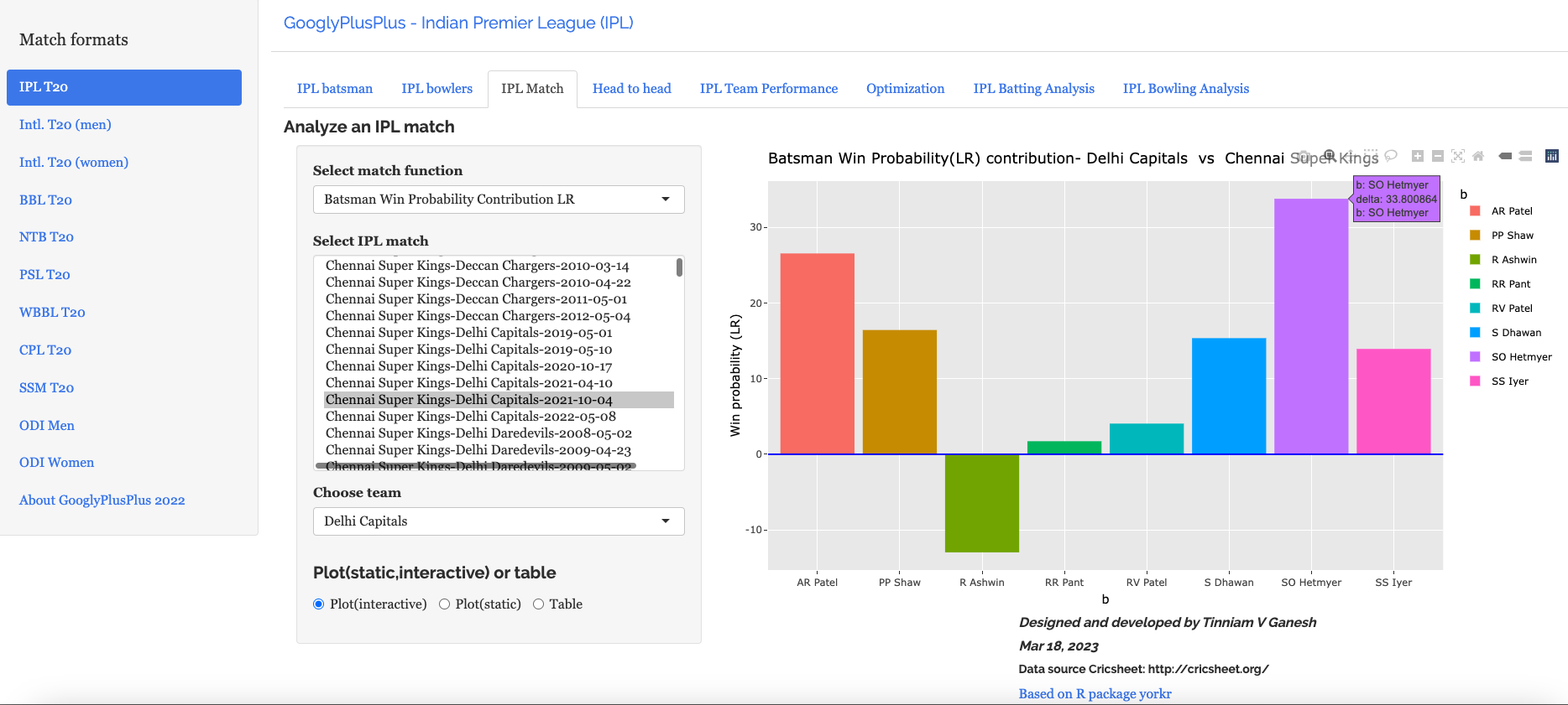
e)Batsman Win Probability contribution:DC – CSK vs DC – 4 Oct 2021
Computing the individual batsman’s Win Contribution and plotting we have. Hetmeyer has a higher Win Probability contribution than Shikhar Dhawan depsite scoring fewer runs
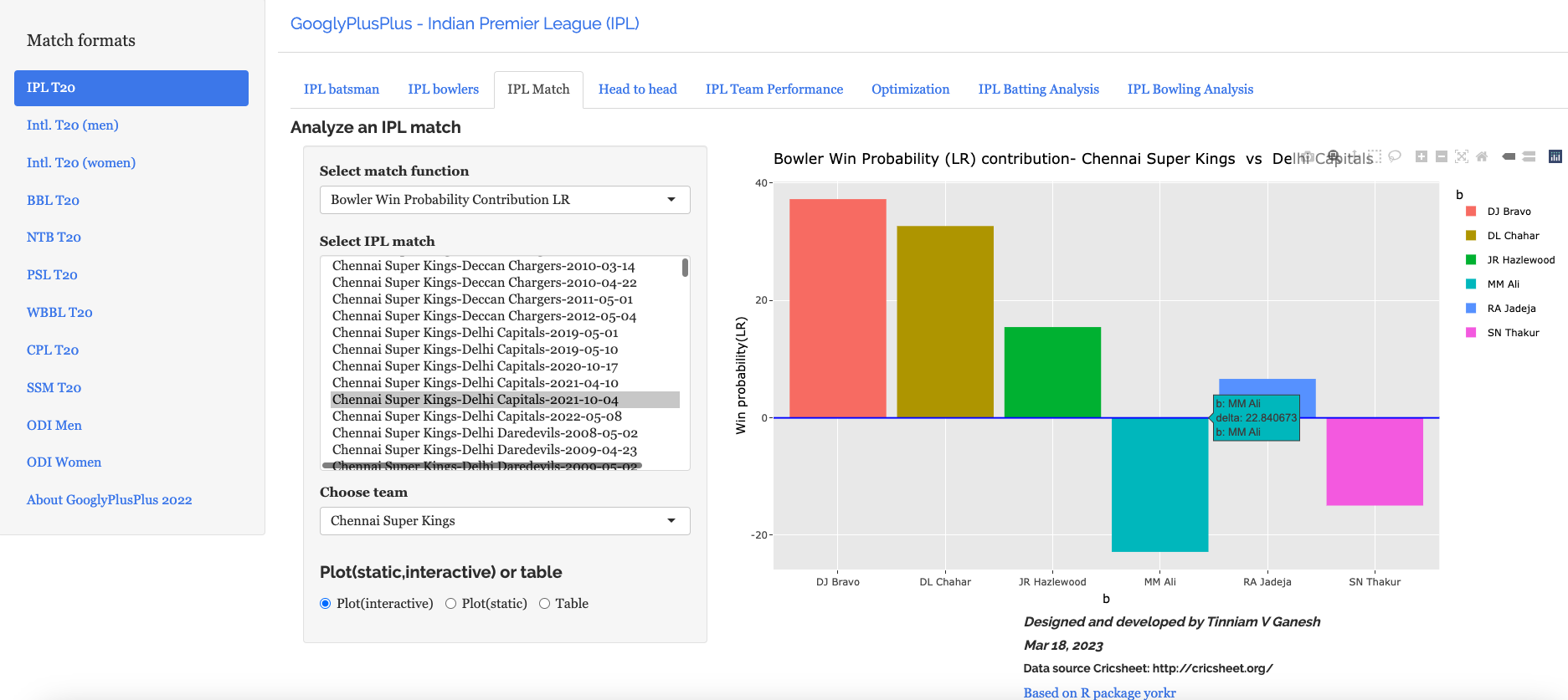
f) Bowler’s Win Probability contribution :CSK – CSK vs DC – 4 Oct 2021
We can also check the Win Probability of the bowlers. So for e.g the CSK bowlers and which bowlers had the most impact. Moeen Ali has the least impact in this match
B) Intl. T20 (men) Australia vs India – 25 Sep 2022
a) Worm wicket chart – Australia vs India – 25 Sep 2022
This was another close match in which India won with the penultimate ball
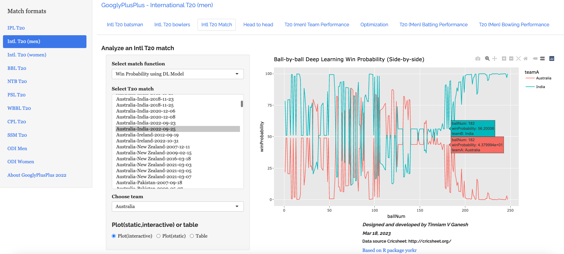
b) Win Probability based on Deep Learning model (side-by-side) –Australia vs India – 25 Sep 2022
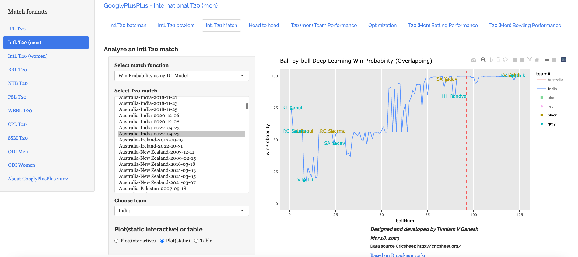
c) Win Probability based on Deep Learning model (overlapping) –Australia vs India – 25 Sep 2022
The plot below shows how the Win Probability of the teams varied across the 20 overs. The 2 Win Probability distributions are superimposed over each other
d) Batsman Win Probability Contribution : India – Australia vs India – 25 Sep 2022
Selectively choosing the India Win Probability plot by double-clicking legend ‘India’ on the right , followed by single click of black, grey legend we have
We see that Kohli, Suryakumar Yadav have good contribution to the Win Probability
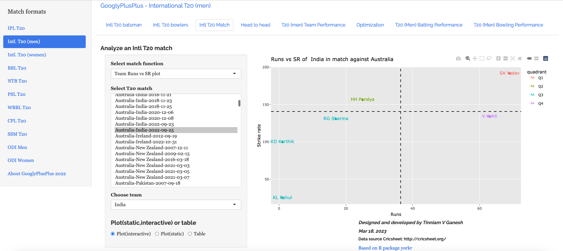
e) Plotting the Runs vs Strike Rate:India – Australia vs India – 25 Sep 2022
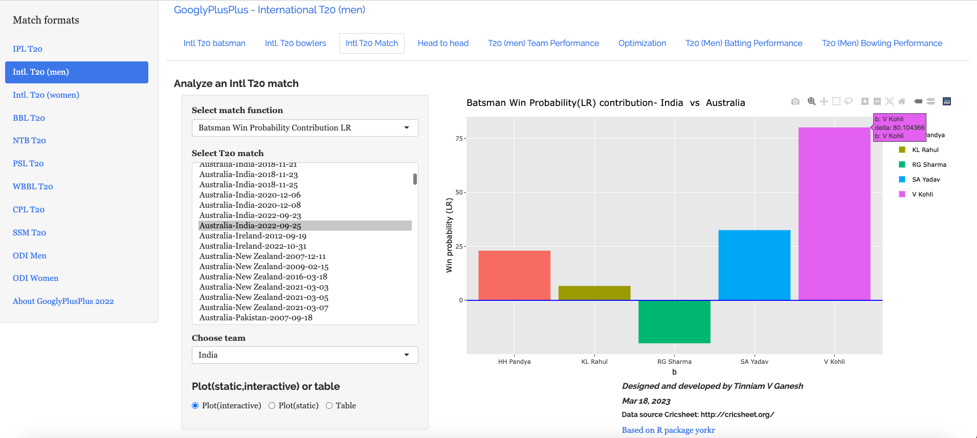
f) Batsman’s Win Probability Contribution-Australia vs India – 25 Sep 2022
Finally plotting the Batsman’s Win Probability Contribution
Interestingly, Kohli has a greater Win Probability Contribution than SKY, though SKY scored more runs at a better strike rate. As mentioned above, the Win Probability is context dependent and also depends on past performances of the player (batsman, bowler)
Finally let us look at
C) India vs England Intll T20 Women (11 July 2021)
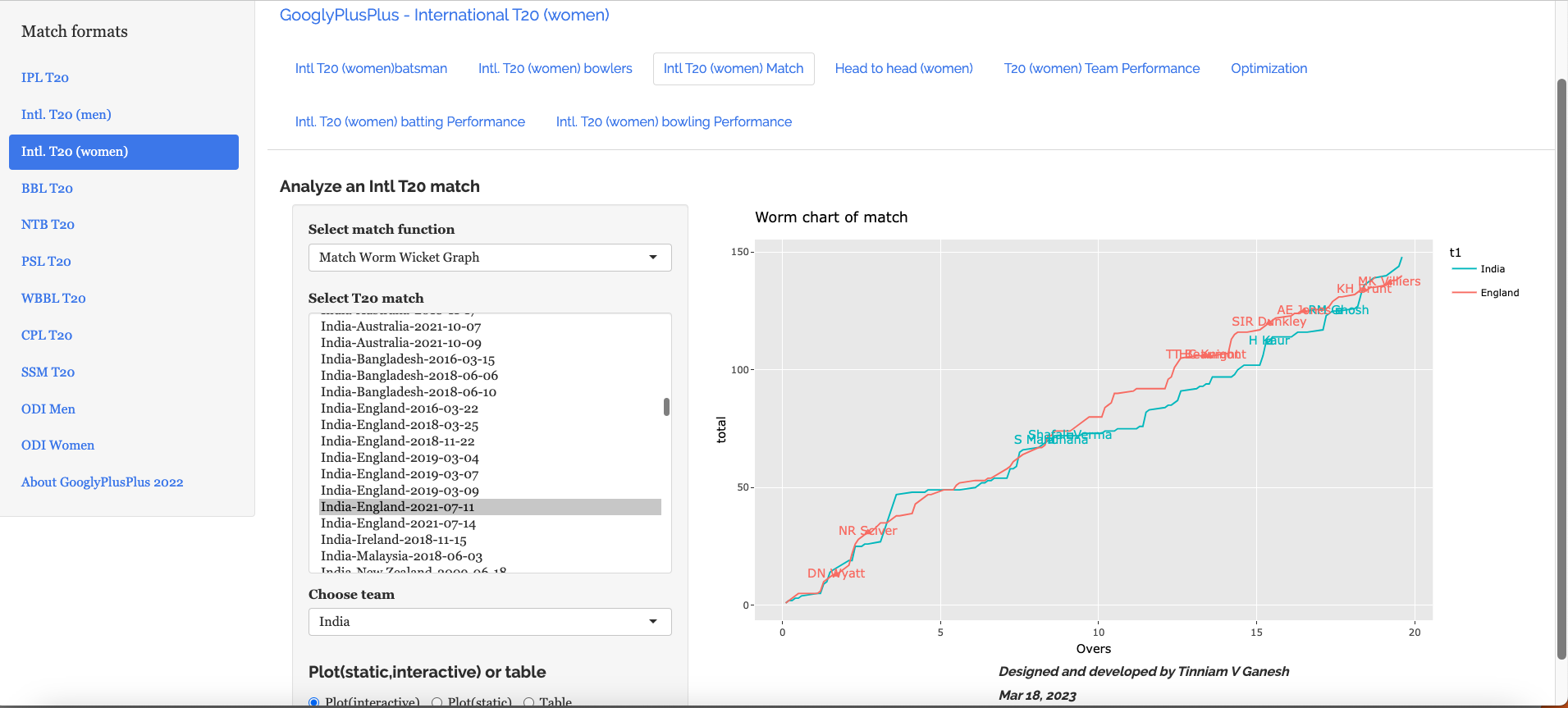
a) Worm wicket chart – India vs England Intl. T20 Women (11 July 2021)
India won this T20 match by 8 runs
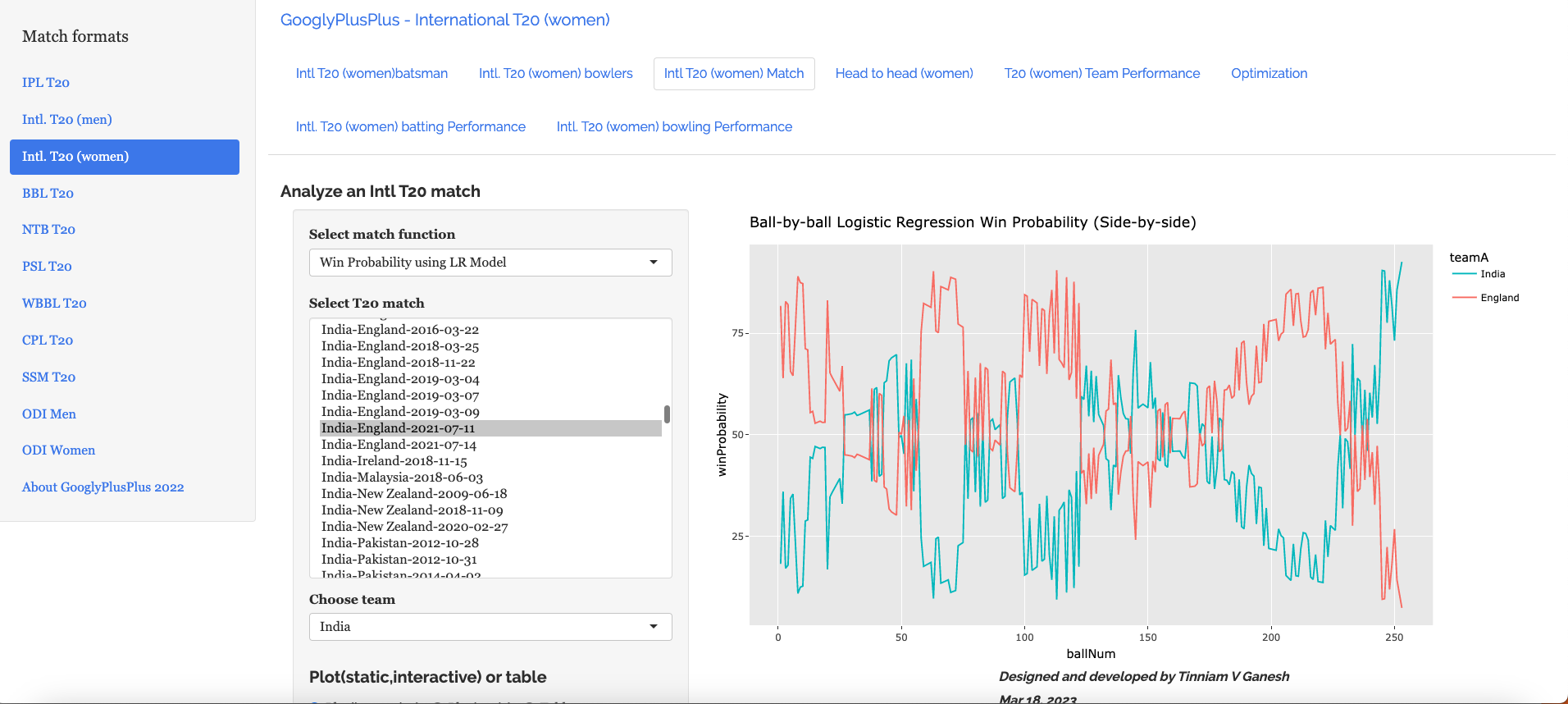
b) Win Probability using the Logistic Regression Model –India vs England Intl. T20 Women (11 July 2021)
c) Win Probability with the DL model –India vs England Intl. T20 Women (11 July 2021)
d) Bowler Win Probability Contribution with the LR model–India vs England Intl. T20 Women (11 July 2021)
e) Bowler Win Contribution with the DL model–India vs England Intl. T20 Women (11 July 2021)
Go ahead and try out the latest version of GooglyPlusPlus
This should be my last post on computing T20 Win Probability. In this post I compute Win Probability using Augmented Data with the help of Conditional Tabular Generative Adversarial Networks (CTGANs).
A.Introduction
I started the computation of T20 match Win Probability in my earlier post
This was lightweight and could be easily deployed in my Shiny GooglyPlusPlus app as opposed to the Tidymodel’s Random Forest, which was bulky and slow.
d) Finally I decided to try and improve the accuracy of my Deep Learning Model using Synthetic data. Towards this end, my explorations led me to Conditional Tabular Generative Adversarial Networks (CTGANs). CTGAN are GAN networks that can be used with Tabular data as GAN models are not useful with tabular data. However, the best performance I got for
DL Keras Model + Synthetic data : accuracy =0.77
The poorer accuracy was because CTGAN requires enormous computing power (GPUs) and RAM. The free version of Colab, Kaggle kept crashing when I tried with even 0.1 % of my 1.2 million dataset size. Finally, I tried with just 0.05% and was able to generate synthetic data. Most likely, it is the small sample size and the smaller number of epochs could be the reason for the poor result. In any case, it was worth trying and this approach would possibly work with sufficient computing resources.
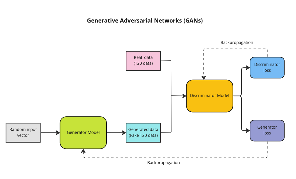
B.Generative Adversarial Networks (GANs)
Generative Adversarial Networks (GANs) was the brain child of Ian Goodfellow who demonstrated it in 2014. GANs are capable of generating synthetic text, tables, images, videos using available data. In Adversarial nets framework, the generative model is pitted against an adversary: a discriminative model that learns to determine whether a sample is from the model distribution or the data distribution.
GANs have 2 Deep Neural Networks , the Generator and Discriminator which compete against other
The Generator (Counterfeiter) takes random noise as input and generates fake images, tables, text. The generator learns to generate plausible data. The generated instances become negative training examples for the discriminator.
The Discriminator (Police) which tries to distinguish between the real and fake images, text. The discriminator learns to distinguish the generator’s fake data from real data. The discriminator penalises the generator for producing implausible results.
A pictorial representation of the GAN model can be shown below
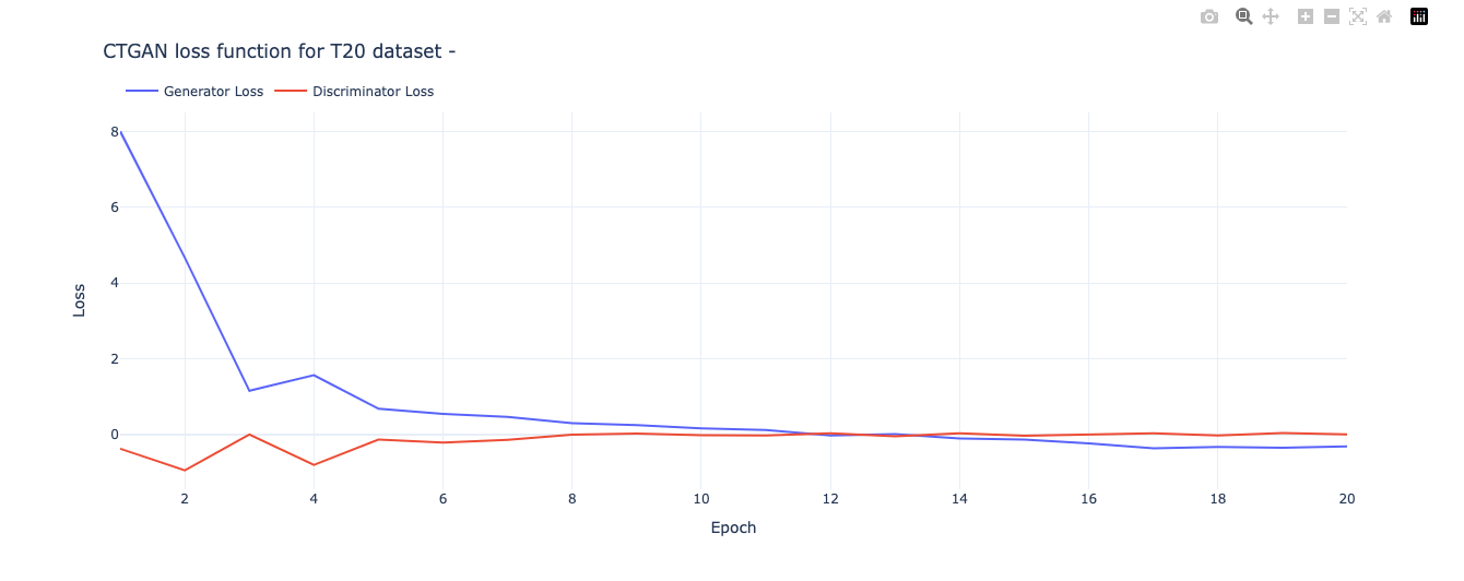
Theoretically best performance of GANs are supposed to happen when the network reaches the ‘Nash equilibrium‘, i.e. when the Generator produces near fake images and the Discriminator’s loss is f ~0.5 i.e. the discriminator is unable to distinguish between real and fake images.
Note: Though I have mentioned T20 data in the above GAN model, the T20 tabular data is actually used in CTGAN which is slightly different from the above. See Reference 2) below.
C. Conditional Tabular Generative Adversial Networks (CTGANs)
“Modeling the probability distribution of rows in tabular data and generating realistic synthetic data is a non-trivial task. Tabular data usually contains a mix of discrete and continuous columns. Continuous columns may have multiple modes whereas discrete columns are sometimes imbalanced making the modeling difficult.” CTGANs handle these challenges.
I came upon CTGAN after spending some time exploring GANs via blogs, videos etc. For building the model I use real T20 match data. However, CTGAN requires immense raw computing power and a lot of RAM. My initial attempts on Colab, my Mac (12 core, 32GB RAM), took forever before eventually crashing, I switched to Kaggle and used GPUs. Still I was only able to use only a miniscule part of my T20 dataset. My match data has 1.2 million rows, hoanything > 0.05% resulted in Kaggle crashing. Since I was able to use only a fraction, I executed the CTGAN model over several iterations, each iteration with a random 0.05% sample of the dataset. At the end of each iterations I also generate synthetic dataset. Over 12 iterations, I generate close 360K of ‘synthetic‘ T20 match data.
I then augment the 1.2 million rows of ‘real‘ T20 match data with the generated ‘synthetic T20 match data to run my Deep Learning model
Here the quality of the synthetic data set is evaluated.
a) Statistical evaluation
Read the real T20 match data
Read the generated T20 synthetic match data
import pandas as pd

# Read the T20 match and synthetic match data
df = pd.read_csv('/kaggle/input/cricket1/t20.csv').  #1.2 million rows
synthetic=pd.read_csv('/kaggle/input/synthetic/synthetic.csv')   #300K

# Randomly sample 1000 rows, and generate stats
df1=df.sample(n=1000)
real=df1.describe()
realData_stats=real.transpose
print(realData_stats)

synthetic1=synthetic.sample(n=1000)
synthetic=synthetic1.describe()
syntheticData_stats=synthetic.transpose
syntheticData_stats
import pandas as pd

# CTGAN prints out a new line for each epoch
epochs_output = str(output).split('\n')

# CTGAN separates the values with commas
raw_values = [line.split(',') for line in epochs_output]
loss_values = pd.DataFrame(raw_values)[:-1] # convert to df and delete last row (empty)

# Rename columns
loss_values.columns = ['Epoch', 'Generator Loss', 'Discriminator Loss']

# Extract the numbers from each column
loss_values['Epoch'] = loss_values['Epoch'].str.extract('(\d+)').astype(int)
loss_values['Generator Loss'] = loss_values['Generator Loss'].str.extract('([-+]?\d*\.\d+|\d+)').astype(float)
loss_values['Discriminator Loss'] = loss_values['Discriminator Loss'].str.extract('([-+]?\d*\.\d+|\d+)').astype(float)

# the result is a row for each epoch that contains the generator and discriminator loss
loss_values.head()
import plotly.graph_objects as go

# Plot loss function
fig = go.Figure(data=[go.Scatter(x=loss_values['Epoch'], y=loss_values['Generator Loss'], name='Generator Loss'),
                      go.Scatter(x=loss_values['Epoch'], y=loss_values['Discriminator Loss'], name='Discriminator Loss')])


# Update the layout for best viewing
fig.update_layout(template='plotly_white',
                    legend_orientation="h",
                    legend=dict(x=0, y=1.1))

title = 'CTGAN loss function for T20 dataset - '
fig.update_layout(title=title, xaxis_title='Epoch', yaxis_title='Loss')
fig.show()
G. Qualitative evaluation of Synthetic data
a) Quality of continuous columns in synthetic data
KSComplement -This metric computes the similarity of a real column vs. a synthetic column in terms of the column shapes.The KSComplement uses the Kolmogorov-Smirnov statistic. Closer to 1.0 is good and 0 is worst
The performance is decent but not excellent. I was unable to execute more epochs as it it required larger than the memory allowed
c) Correlation similarity
This metric measures the correlation between a pair of numerical columns and computes the similarity between the real and synthetic data – it compares the trends of 2D distributions. Best 1.0 and 0.0 is worst
In this final part I augment my T20 match data set with the generated synthetic T20 data set.
import pandas as pd
from numpy import savetxt
import tensorflow as tf
from tensorflow import keras
import pandas as pd
import numpy as np


from keras.layers import Input, Embedding, Flatten, Dense, Reshape, Concatenate, Dropout
from keras.models import Model
import matplotlib.pyplot as plt

# Read real and synthetic data
df = pd.read_csv('/kaggle/input/cricket1/t20.csv')
synthetic=pd.read_csv('/kaggle/input/synthetic/synthetic.csv')

# Augment the data. Concatenate real & synthetic data
df1=pd.concat([df,synthetic])

# Create training and test samples
print("Shape of dataframe=",df1.shape)
train_dataset = df1.sample(frac=0.8,random_state=0)
test_dataset = df1.drop(train_dataset.index)
train_dataset1 = train_dataset[['batsmanIdx','bowlerIdx','ballNum','ballsRemaining','runs','runRate','numWickets','runsMomentum','perfIndex']]
test_dataset1 = test_dataset[['batsmanIdx','bowlerIdx','ballNum','ballsRemaining','runs','runRate','numWickets','runsMomentum','perfIndex']]
train_dataset1
train_labels = train_dataset.pop('isWinner')
test_labels = test_dataset.pop('isWinner')
print(train_dataset1.shape)

a=train_dataset1.describe()
stats=a.transpose
print(a)
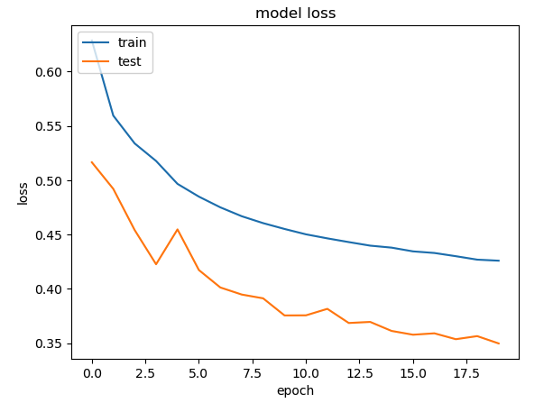
As can be seen the accuracy with augmented dataset is around 0.77, while without it I was getting 0.867 with just the real data. This degradation is probably due to the folllowing reasons
Only a fraction of the dataset was used for training. This was not representative of the data distribution for CTGAN to correctly synthesise data
The number of epochs had to be kept low to prevent Kaggle/Colab from crashing
I. Conclusion
This post shows how we can generate synthetic T20 match data to augment real T20 match data. Assuming we have sufficient processing power we should be able to generate synthetic data for augmenting our data set. This should improve the accuracy of the Win Probabily Deep Learning model.