cricketr digs the Ashes!

Published in R bloggers: cricketr digs the Ashes

Introduction

In some circles the Ashes is considered the ‘mother of all cricketing battles’. But, being a staunch supporter of all things Indian, cricket or otherwise, I have to say that the Ashes pales in comparison against a India-Pakistan match. After all, what are a few frowns and raised eyebrows at the Ashes in comparison to the seething emotions and reckless exuberance of Indian fans.

Anyway, the Ashes are an interesting duel and I have decided to do some cricketing analysis using my R package cricketr. For this analysis I have chosen the top 2 batsman and top 2 bowlers from both the Australian and English sides.

Batsmen

  1. Steven Smith (Aus) – Innings – 58 , Ave: 58.52, Strike Rate: 55.90
  2. David Warner (Aus) – Innings – 76, Ave: 46.86, Strike Rate: 73.88
  3. Alistair Cook (Eng) – Innings – 208 , Ave: 46.62, Strike Rate: 46.33
  4. J E Root (Eng) – Innings – 53, Ave: 54.02, Strike Rate: 51.30

Bowlers

  1. Mitchell Johnson (Aus) – Innings-131, Wickets – 299, Econ Rate : 3.28
  2. Peter Siddle (Aus) – Innings – 104 , Wickets- 192, Econ Rate : 2.95
  3. James Anderson (Eng) – Innings – 199 , Wickets- 406, Econ Rate : 3.05
  4. Stuart Broad (Eng) – Innings – 148 , Wickets- 296, Econ Rate : 3.08

It is my opinion if any 2 of the 4 in either team click then they will be able to swing the match in favor of their team.

I have interspersed the plots with a few comments. Feel free to draw your conclusions!

If you are passionate about cricket, and love analyzing cricket performances, then check out my racy book on cricket ‘Cricket analytics with cricketr and cricpy – Analytics harmony with R & Python’! This book discusses and shows how to use my R package ‘cricketr’ and my Python package ‘cricpy’ to analyze batsmen and bowlers in all formats of the game (Test, ODI and T20). The paperback is available on Amazon at $21.99 and  the kindle version at $9.99/Rs 449/-. A must read for any cricket lover! Check it out!!

You can download the latest PDF version of the book  at  ‘Cricket analytics with cricketr and cricpy: Analytics harmony with R and Python-6th edition

Untitled

cks), and $4.99/Rs 320 and $6.99/Rs448 respectively

Important note 1: The latest release of ‘cricketr’ now includes the ability to analyze performances of teams now!!  See Cricketr adds team analytics to its repertoire!!!

Important note 2 : Cricketr can now do a more fine-grained analysis of players, see Cricketr learns new tricks : Performs fine-grained analysis of players

Important note 3: Do check out the python avatar of cricketr, ‘cricpy’ in my post ‘Introducing cricpy:A python package to analyze performances of cricketers

The analysis is included below. Note: This post has also been hosted at Rpubs as cricketr digs the Ashes!
You can also download this analysis as a PDF file from cricketr digs the Ashes!

Do check out my interactive Shiny app implementation using the cricketr package – Sixer – R package cricketr’s new Shiny avatar

Note: If you would like to do a similar analysis for a different set of batsman and bowlers, you can clone/download my skeleton cricketr template from Github (which is the R Markdown file I have used for the analysis below). You will only need to make appropriate changes for the players you are interested in. Just a familiarity with R and R Markdown only is needed.

Important note: Do check out my other posts using cricketr at cricketr-posts

The package can be installed directly from CRAN

if (!require("cricketr")){ 
    install.packages("cricketr",lib = "c:/test") 
} 
library(cricketr)

or from Github

library(devtools)
install_github("tvganesh/cricketr")
library(cricketr)

Analyses of Batsmen

The following plots gives the analysis of the 2 Australian and 2 English batsmen. It must be kept in mind that Cooks has more innings than all the rest put together. Smith has the best average, and Warner has the best strike rate

Box Histogram Plot

This plot shows a combined boxplot of the Runs ranges and a histogram of the Runs Frequency

batsmanPerfBoxHist("./smith.csv","S Smith")

swcr-boxhist-1

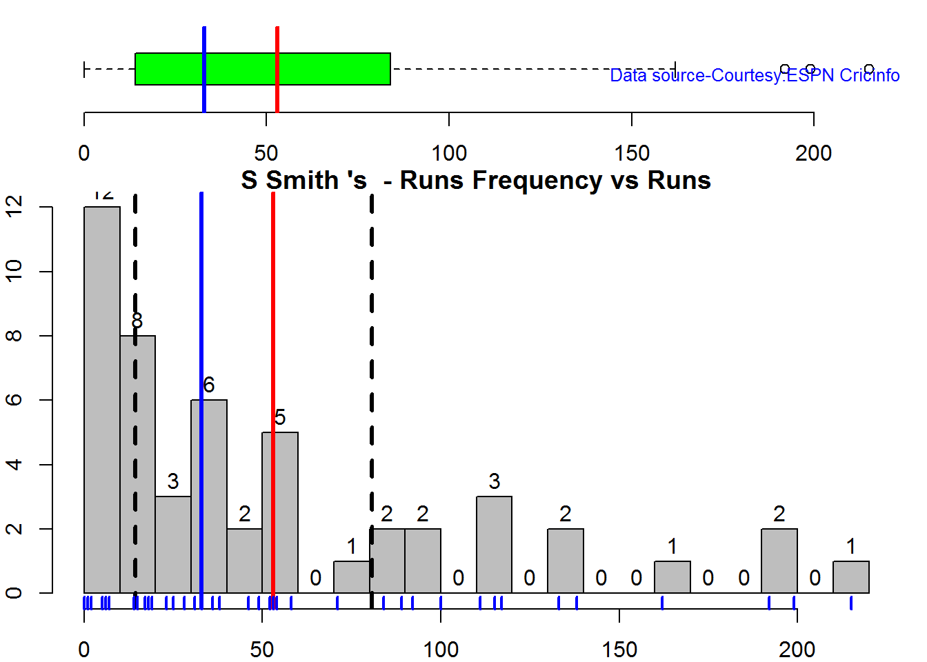
batsmanPerfBoxHist("./warner.csv","D Warner")

swcr-boxhist-2

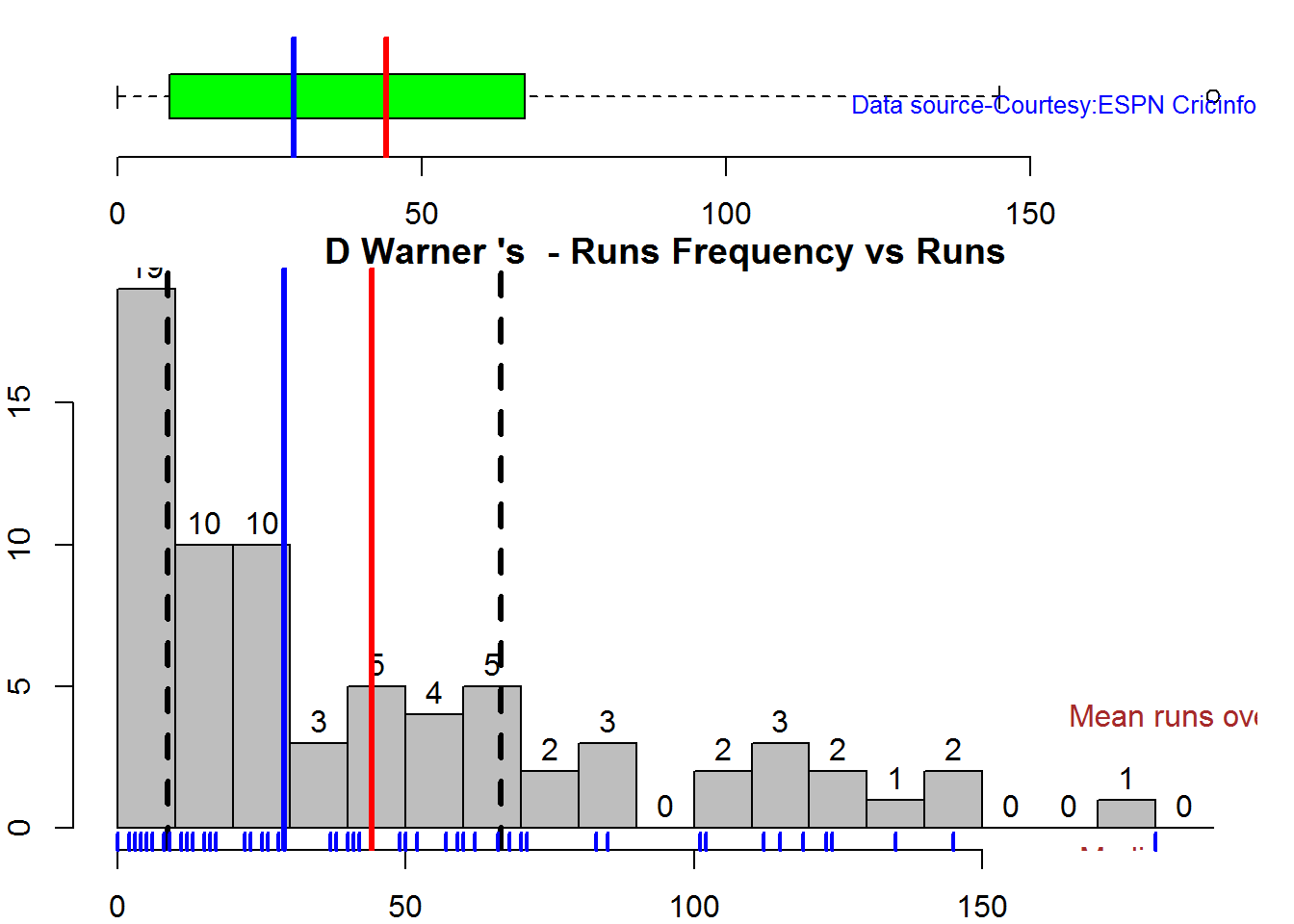
batsmanPerfBoxHist("./cook.csv","A Cook")

swcr-boxhist-3

batsmanPerfBoxHist("./root.csv","JE Root")

swcr-boxhist-4

Plot os 4s, 6s and the type of dismissals

A. Steven Smith

par(mfrow=c(1,3))
par(mar=c(4,4,2,2))
batsman4s("./smith.csv","S Smith")
batsman6s("./smith.csv","S Smith")
batsmanDismissals("./smith.csv","S Smith")

smith-4s6sout-1

dev.off()
## null device 
##           1

B. David Warner

par(mfrow=c(1,3))
par(mar=c(4,4,2,2))
batsman4s("./warner.csv","D Warner")
batsman6s("./warner.csv","D Warner")
batsmanDismissals("./warner.csv","D Warner")

warner-4s6sout-1

dev.off()
## null device 
##           1

C. Alistair Cook

par(mfrow=c(1,3))
par(mar=c(4,4,2,2))
batsman4s("./cook.csv","A Cook")
batsman6s("./cook.csv","A Cook")
batsmanDismissals("./cook.csv","A Cook")
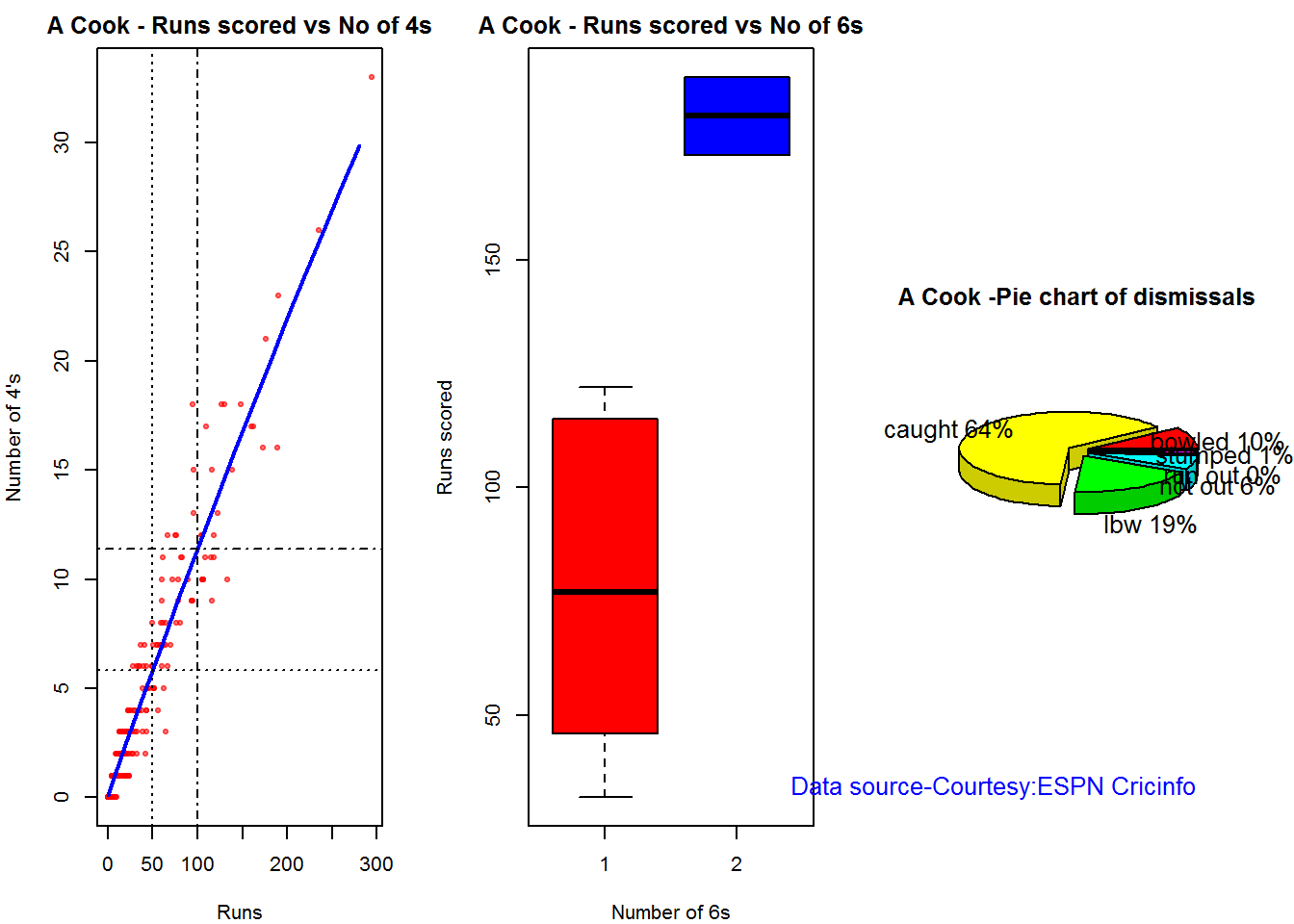
cook-4s6sout-1

dev.off()
## null device 
##           1

D. J E Root

par(mfrow=c(1,3))
par(mar=c(4,4,2,2))
batsman4s("./root.csv","JE Root")
batsman6s("./root.csv","JE Root")
batsmanDismissals("./root.csv","JE Root")

root-4s6sout-1

dev.off()
## null device 
##           1

Relative Mean Strike Rate

In this first plot I plot the Mean Strike Rate of the batsmen. It can be Warner’s has the best strike rate (hit outside the plot!) followed by Smith in the range 20-100. Root has a good strike rate above hundred runs. Cook maintains a good strike rate.

par(mar=c(4,4,2,2))
frames <- list("./smith.csv","./warner.csv","cook.csv","root.csv")
names <- list("Smith","Warner","Cook","Root")
relativeBatsmanSR(frames,names)

plot-1-1

Relative Runs Frequency Percentage

The plot below show the percentage contribution in each 10 runs bucket over the entire career.It can be seen that Smith pops up above the rest with remarkable regularity.COok is consistent over the entire range.

frames <- list("./smith.csv","./warner.csv","cook.csv","root.csv")
names <- list("Smith","Warner","Cook","Root")
relativeRunsFreqPerf(frames,names)

plot-2-1

Moving Average of runs over career

The moving average for the 4 batsmen indicate the following 1. S Smith is the most promising. There is a marked spike in Performance. Cook maintains a steady pace and is consistent over the years averaging 50 over the years.

par(mfrow=c(2,2))
par(mar=c(4,4,2,2))
batsmanMovingAverage("./smith.csv","S Smith")
batsmanMovingAverage("./warner.csv","D Warner")
batsmanMovingAverage("./cook.csv","A Cook")
batsmanMovingAverage("./root.csv","JE Root")
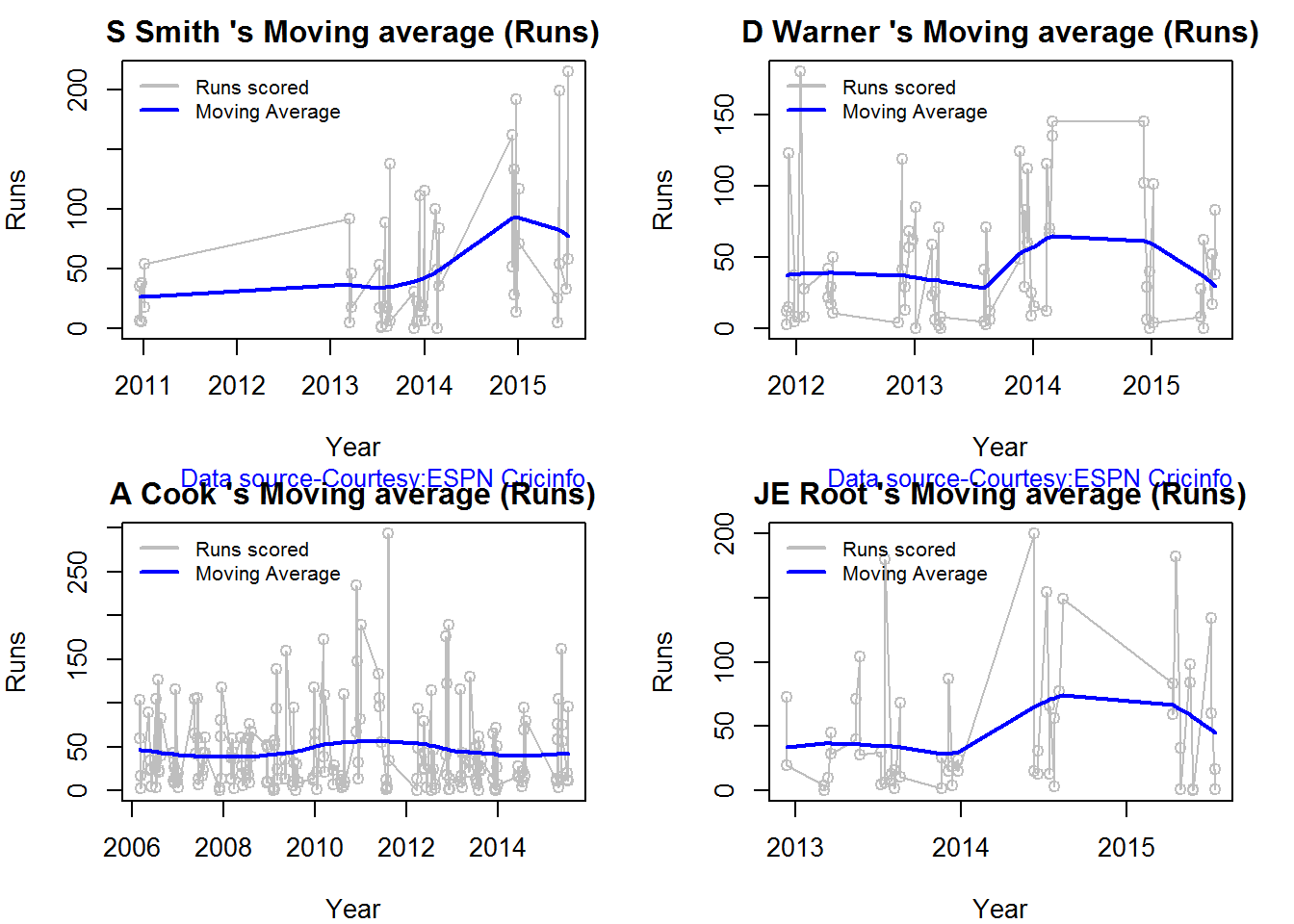
swcr-ma-1

dev.off()
## null device 
##           1

Runs forecast

The forecast for the batsman is shown below. As before Cooks’s performance is really consistent across the years and the forecast is good for the years ahead. In Cook’s case it can be seen that the forecasted and actual runs are reasonably accurate

par(mfrow=c(2,2))
par(mar=c(4,4,2,2))
batsmanPerfForecast("./smith.csv","S Smith")
batsmanPerfForecast("./warner.csv","D Warner")
batsmanPerfForecast("./cook.csv","A Cook")
## Warning in HoltWinters(ts.train): optimization difficulties: ERROR:
## ABNORMAL_TERMINATION_IN_LNSRCH
batsmanPerfForecast("./root.csv","JE Root")

swcr-perf-1

dev.off()
## null device 
##           1

3D plot of Runs vs Balls Faced and Minutes at Crease

The plot is a scatter plot of Runs vs Balls faced and Minutes at Crease. A prediction plane is fitted

par(mfrow=c(1,2))
par(mar=c(4,4,2,2))
battingPerf3d("./smith.csv","S Smith")
battingPerf3d("./warner.csv","D Warner")
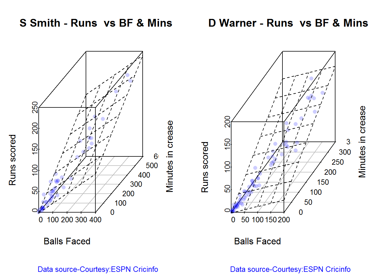
plot-3-1

par(mfrow=c(1,2))
par(mar=c(4,4,2,2))
battingPerf3d("./cook.csv","A Cook")
battingPerf3d("./root.csv","JE Root")

plot-4-1

dev.off()
## null device 
##           1

Predicting Runs given Balls Faced and Minutes at Crease

A multi-variate regression plane is fitted between Runs and Balls faced +Minutes at crease.

BF <- seq( 10, 400,length=15)
Mins <- seq(30,600,length=15)
newDF <- data.frame(BF,Mins)
smith <- batsmanRunsPredict("./smith.csv","S Smith",newdataframe=newDF)
warner <- batsmanRunsPredict("./warner.csv","D Warner",newdataframe=newDF)
cook <- batsmanRunsPredict("./cook.csv","A Cook",newdataframe=newDF)
root <- batsmanRunsPredict("./root.csv","JE Root",newdataframe=newDF)

The fitted model is then used to predict the runs that the batsmen will score for a given Balls faced and Minutes at crease. It can be seen that Warner sets a searing pace in the predicted runs for a given Balls Faced and Minutes at crease while Smith and Root are neck to neck in the predicted runs

batsmen <-cbind(round(smith$Runs),round(warner$Runs),round(cook$Runs),round(root$Runs))
colnames(batsmen) <- c("Smith","Warner","Cook","Root")
newDF <- data.frame(round(newDF$BF),round(newDF$Mins))
colnames(newDF) <- c("BallsFaced","MinsAtCrease")
predictedRuns <- cbind(newDF,batsmen)
predictedRuns
##    BallsFaced MinsAtCrease Smith Warner Cook Root
## 1          10           30     9     12    6    9
## 2          38           71    25     33   20   25
## 3          66          111    42     53   33   42
## 4          94          152    58     73   47   59
## 5         121          193    75     93   60   75
## 6         149          234    91    114   74   92
## 7         177          274   108    134   88  109
## 8         205          315   124    154  101  125
## 9         233          356   141    174  115  142
## 10        261          396   158    195  128  159
## 11        289          437   174    215  142  175
## 12        316          478   191    235  155  192
## 13        344          519   207    255  169  208
## 14        372          559   224    276  182  225
## 15        400          600   240    296  196  242

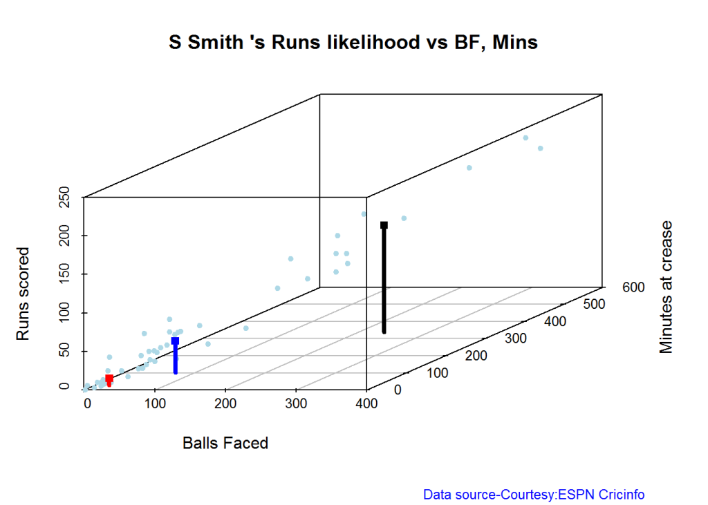
Highest runs likelihood

The plots below the runs likelihood of batsman. This uses K-Means. It can be seen Smith has the best likelihood around 40% of scoring around 41 runs, followed by Root who has 28.3% likelihood of scoring around 81 runs

A. Steven Smith

batsmanRunsLikelihood("./smith.csv","S Smith")
smith-1
## Summary of  S Smith 's runs scoring likelihood
## **************************************************
## 
## There is a 40 % likelihood that S Smith  will make  41 Runs in  73 balls over 101  Minutes 
## There is a 36 % likelihood that S Smith  will make  9 Runs in  21 balls over  27  Minutes 
## There is a 24 % likelihood that S Smith  will make  139 Runs in  237 balls over 338  Minutes

B. David Warner

batsmanRunsLikelihood("./warner.csv","D Warner")
warner-1
## Summary of  D Warner 's runs scoring likelihood
## **************************************************
## 
## There is a 11.11 % likelihood that D Warner  will make  134 Runs in  159 balls over 263  Minutes 
## There is a 63.89 % likelihood that D Warner  will make  17 Runs in  25 balls over  37  Minutes 
## There is a 25 % likelihood that D Warner  will make  73 Runs in  105 balls over 156  Minutes

C. Alastair Cook

batsmanRunsLikelihood("./cook.csv","A Cook")
cook,cache-TRUE-1
## Summary of  A Cook 's runs scoring likelihood
## **************************************************
## 
## There is a 27.72 % likelihood that A Cook  will make  64 Runs in  140 balls over 195  Minutes 
## There is a 59.9 % likelihood that A Cook  will make  15 Runs in  32 balls over  46  Minutes 
## There is a 12.38 % likelihood that A Cook  will make  141 Runs in  300 balls over 420  Minutes

D. J E Root

batsmanRunsLikelihood("./root.csv","JE Root")
oot-1
## Summary of  JE Root 's runs scoring likelihood
## **************************************************
## 
## There is a 28.3 % likelihood that JE Root  will make  81 Runs in  158 balls over 223  Minutes 
## There is a 7.55 % likelihood that JE Root  will make  179 Runs in  290 balls over  425  Minutes 
## There is a 64.15 % likelihood that JE Root  will make  16 Runs in  39 balls over 59  Minutes
 

Average runs at ground and against opposition

A. Steven Smith

par(mfrow=c(1,2))
par(mar=c(4,4,2,2))
batsmanAvgRunsGround("./smith.csv","S Smith")
batsmanAvgRunsOpposition("./smith.csv","S Smith")
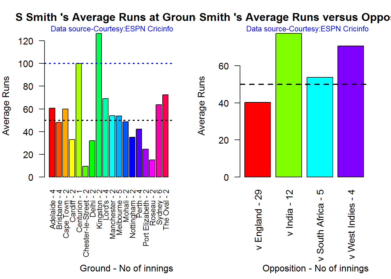
avgrg-1-1

dev.off()
## null device 
##           1

B. David Warner

par(mfrow=c(1,2))
par(mar=c(4,4,2,2))
batsmanAvgRunsGround("./warner.csv","D Warner")
batsmanAvgRunsOpposition("./warner.csv","D Warner")
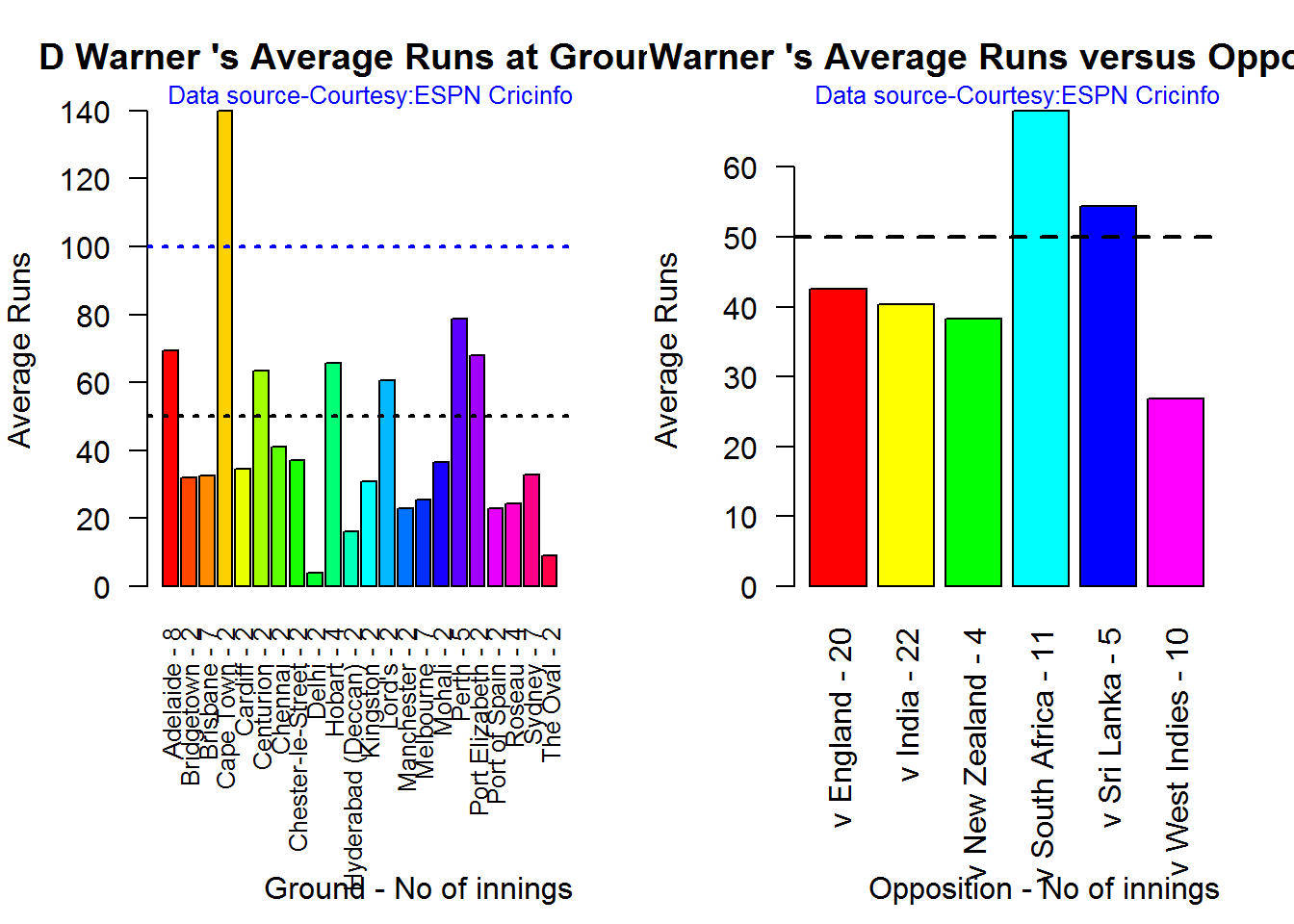
avgrg-2-1

dev.off()
## null device 
##           1

C. Alistair Cook

par(mfrow=c(1,2))
par(mar=c(4,4,2,2))
batsmanAvgRunsGround("./cook.csv","A Cook")
batsmanAvgRunsOpposition("./cook.csv","A Cook")

avgrg-3-1

dev.off()
## null device 
##           1

D. J E Root

par(mfrow=c(1,2))
par(mar=c(4,4,2,2))
batsmanAvgRunsGround("./root.csv","JE Root")
batsmanAvgRunsOpposition("./root.csv","JE Root")
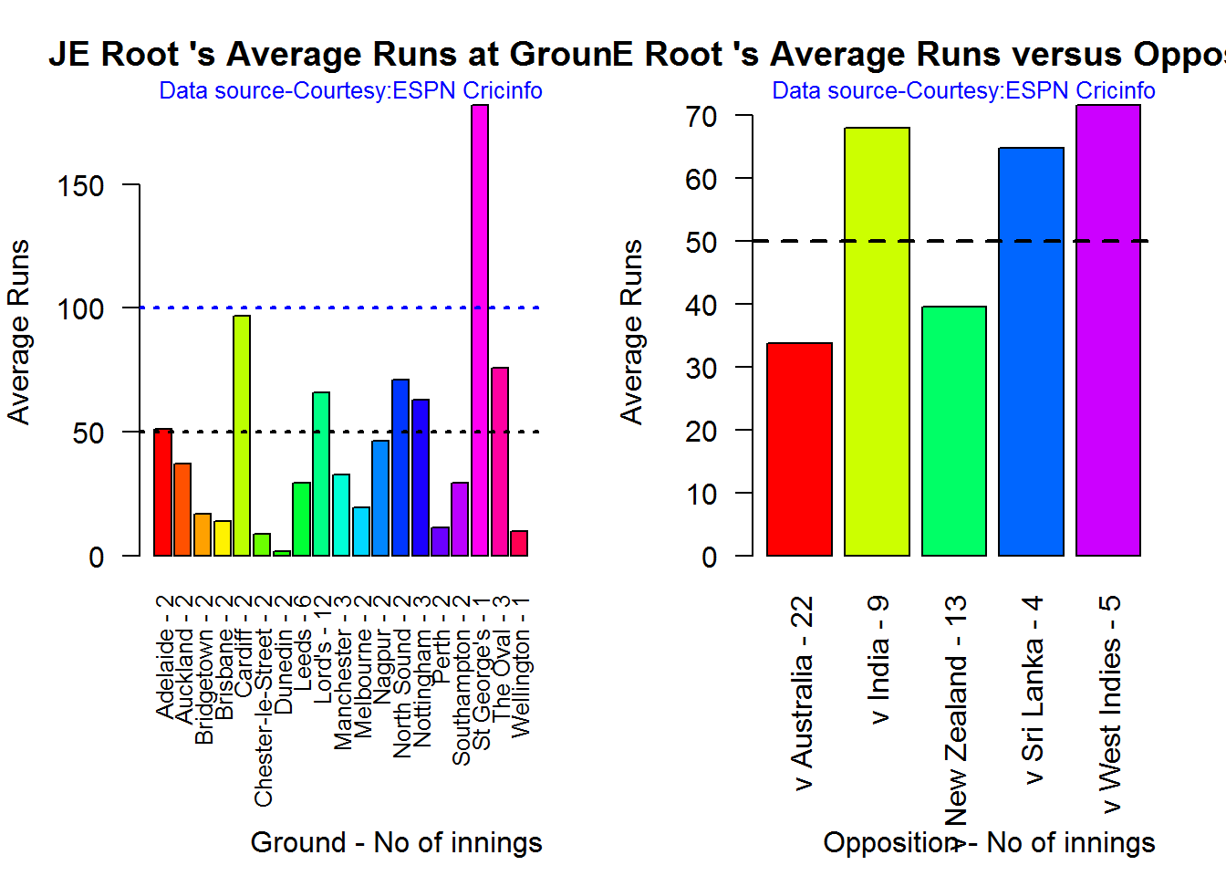
avgrg-4-1

dev.off()
## null device 
##           1

Analysis of bowlers

  1. Mitchell Johnson (Aus) – Innings-131, Wickets – 299, Econ Rate : 3.28
  2. Peter Siddle (Aus) – Innings – 104 , Wickets- 192, Econ Rate : 2.95
  3. James Anderson (Eng) – Innings – 199 , Wickets- 406, Econ Rate : 3.05
  4. Stuart Broad (Eng) – Innings – 148 , Wickets- 296, Econ Rate : 3.08

Anderson has the highest number of inning and wickets followed closely by Broad and Mitchell who are in a neck to neck race with respect to wickets. Johnson is on the more expensive side though. Siddle has fewer innings but a good economy rate.

Wicket Frequency percentage

This plot gives the percentage of wickets for each wickets (1,2,3…etc)

par(mfrow=c(1,4))
par(mar=c(4,4,2,2))
bowlerWktsFreqPercent("./johnson.csv","Johnson")
bowlerWktsFreqPercent("./siddle.csv","Siddle")
bowlerWktsFreqPercent("./broad.csv","Broad")
bowlerWktsFreqPercent("./anderson.csv","Anderson")
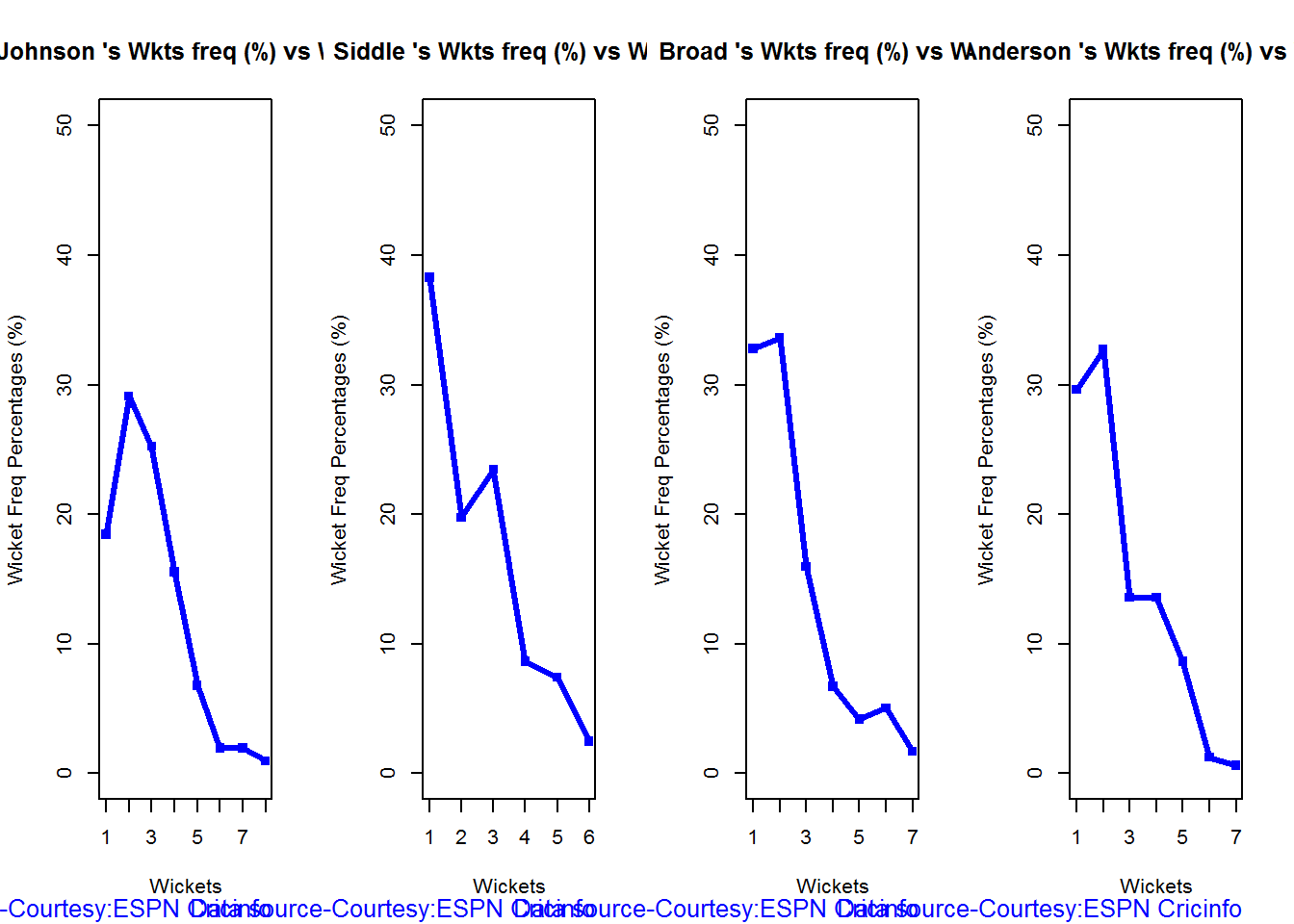
relBowlFP-1

dev.off()
## null device 
##           1

Wickets Runs plot

The plot below gives a boxplot of the runs ranges for each of the wickets taken by the bowlers

par(mfrow=c(1,4))
par(mar=c(4,4,2,2))
bowlerWktsRunsPlot("./johnson.csv","Johnson")
bowlerWktsRunsPlot("./siddle.csv","Siddle")
bowlerWktsRunsPlot("./broad.csv","Broad")
bowlerWktsRunsPlot("./anderson.csv","Anderson")

wktsrun-1

dev.off()
## null device 
##           1

Average wickets in different grounds and opposition

A. Mitchell Johnson

par(mfrow=c(1,2))
par(mar=c(4,4,2,2))
bowlerAvgWktsGround("./johnson.csv","Johnson")
bowlerAvgWktsOpposition("./johnson.csv","Johnson")

gr-1-1

dev.off()
## null device 
##           1

B. Peter Siddle

par(mfrow=c(1,2))
par(mar=c(4,4,2,2))
bowlerAvgWktsGround("./siddle.csv","Siddle")
bowlerAvgWktsOpposition("./siddle.csv","Siddle")

gr-2-1

dev.off()
## null device 
##           1

C. Stuart Broad

par(mfrow=c(1,2))
par(mar=c(4,4,2,2))
bowlerAvgWktsGround("./broad.csv","Broad")
bowlerAvgWktsOpposition("./broad.csv","Broad")

gr-3-1

dev.off()
## null device 
##           1

D. James Anderson

par(mfrow=c(1,2))
par(mar=c(4,4,2,2))
bowlerAvgWktsGround("./anderson.csv","Anderson")
bowlerAvgWktsOpposition("./anderson.csv","Anderson")

gr-4-1

dev.off()
## null device 
##           1

Relative bowling performance

The plot below shows that Mitchell Johnson is the mopst effective bowler among the lot with a higher wickets in the 3-6 wicket range. Broad and Anderson seem to perform well in 2 wickets in comparison to Siddle but in 3 wickets Siddle is better than Broad and Anderson.

frames <- list("./johnson.csv","./siddle.csv","broad.csv","anderson.csv")
names <- list("Johnson","Siddle","Broad","Anderson")
relativeBowlingPerf(frames,names)

relBowlPerf-1

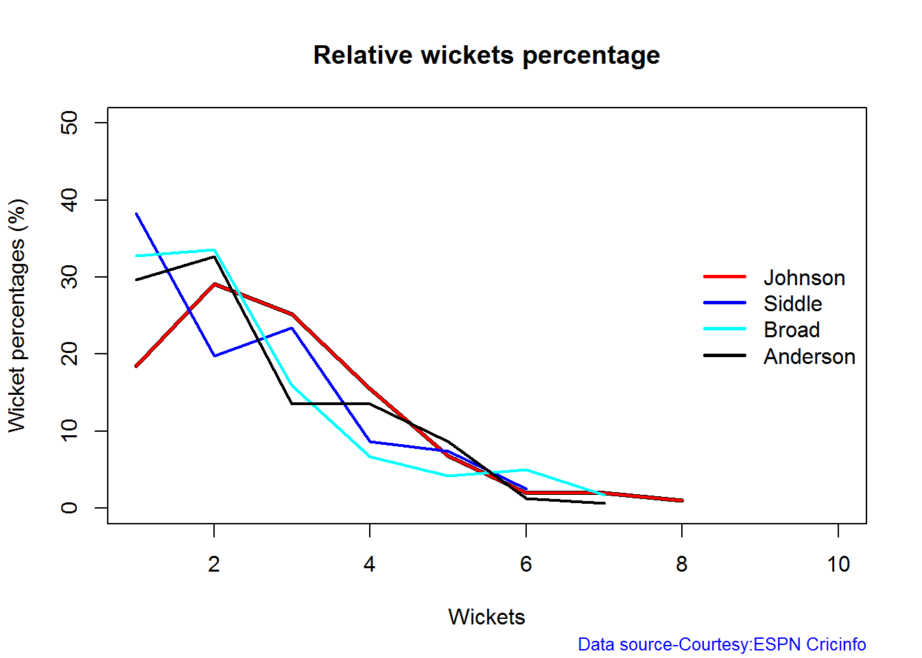
Relative Economy Rate against wickets taken

Anderson followed by Siddle has the best economy rates. Johnson is fairly expensive in the 4-8 wicket range.

frames <- list("./johnson.csv","./siddle.csv","broad.csv","anderson.csv")
names <- list("Johnson","Siddle","Broad","Anderson")
relativeBowlingER(frames,names)

relBowlER-1

Moving average of wickets over career

Johnson is on his second peak while Siddle is on the decline with respect to bowling. Broad and Anderson show improving performance over the years.

par(mfrow=c(2,2))
par(mar=c(4,4,2,2))
bowlerMovingAverage("./johnson.csv","Johnson")
bowlerMovingAverage("./siddle.csv","Siddle")
bowlerMovingAverage("./broad.csv","Broad")
bowlerMovingAverage("./anderson.csv","Anderson")
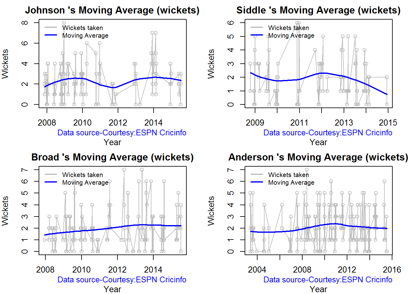
jsba-bowlma-1

dev.off()
## null device 
##           1

Wickets forecast

par(mfrow=c(2,2))
par(mar=c(4,4,2,2))
bowlerPerfForecast("./johnson.csv","Johnson")
bowlerPerfForecast("./siddle.csv","Siddle")
bowlerPerfForecast("./broad.csv","Broad")
bowlerPerfForecast("./anderson.csv","Anderson")

jsba-bowlma-1

dev.off()
## null device 
##           1

Key findings

Here are some key conclusions

  1. Cook has the most number of innings and has been extremly consistent in his scores
  2. Warner has the best strike rate among the lot followed by Smith and Root
  3. The moving average shows a marked improvement over the years for Smith
  4. Johnson is the most effective bowler but is fairly expensive
  5. Anderson has the best economy rate followed by Siddle
  6. Johnson is at his second peak with respect to bowling while Broad and Anderson maintain a steady line and length in their career bowling performance


Also see my other posts in R

  1. Introducing cricketr! : An R package to analyze performances of cricketers
  2. Taking cricketr for a spin – Part 1
  3. A peek into literacy in India: Statistical Learning with R
  4. A crime map of India in R – Crimes against women
  5. Analyzing cricket’s batting legends – Through the mirage with R
  6. Masters of Spin: Unraveling the web with R
  7. Mirror, mirror . the best batsman of them all?

You may also like

  1. A crime map of India in R: Crimes against women
  2. What’s up Watson? Using IBM Watson’s QAAPI with Bluemix, NodeExpress – Part 1
  3. Bend it like Bluemix, MongoDB with autoscaling – Part 2
  4. Informed choices through Machine Learning : Analyzing Kohli, Tendulkar and Dravid
  5. Thinking Web Scale (TWS-3): Map-Reduce – Bring compute to data
  6. Deblurring with OpenCV:Weiner filter reloaded

The moving edge of computing

Published in The Hindu – 30 Sep 2012 as “Three computing technologies that will power the world

“The moving edge of computing computes and having computed moves on…” We could thus rephrase the Rubaiyat of Omar Khayyam’s “The moving hand…” Computing technology has really advanced by leaps and bounds. We are now in a new era of computing. We are in the midst of “intelligent and cognitive” computing.

From the initial days of number crunching by languages of FORTRAN, to the procedural methodology of Pascal or C and later the object oriented paradigm of C++ and Java we have now come a long way.  In this age of information overload technologies that can just solve problems through steps & procedures are no longer adequate. We need technology to detect complex patterns, trends, understand nuances in human language and to automatically resolve problems. In this new era of computing the following 3 technologies are furthering the frontiers of computing technology.

Predictive Analytics

By 2016 130 Exabyte’s (130 * 2 ^ 60) will rip through the internet. The number of mobile devices will exceed the human population this year, 2012 and by 2016 the number of connected devices will touch almost 10 billion. The devices connected to the net will range from mobiles, laptops, tablets, sensors and the millions of devices based on the “internet of things”. All these devices will constantly spew data on the internet. A hot and happening trend in computing is the ability to make business and strategic decisions by determining patterns, trends and outliers among mountains of data. Predictive analytics will be a key discipline in our future and experts will be much sought after. Predictive analytics uses statistical methods to mine intelligence, information and patterns in structured, unstructured and streams of data. Predictive analytics will be applied across many domains from banking, insurance, retail, telecom, energy. There are also applications for energy grids, water management, besides determining user sentiment by mining data from social networks etc.

Cognitive Computing

The most famous technological product in the domain of cognitive computing is IBM’s supercomputer Watson. IBM’s Watson is an artificial intelligence computer system capable of answering questions posed in natural language. IBM’s supercomputer Watson is best known for successfully trouncing a national champion in the popular US TV quiz competition, Jeopardy. What makes this victory more astonishing is that IBM’s Watson had to successfully decipher the nuances of natural language and pick the correct answer.  Following the success at Jeopardy, IBM’s Watson supercomputer has now  been employed by a leading medical insurance firm in US to diagnose medical illnesses and to recommend treatment options for patients. Watson will be able to analyze 1 million books, or roughly 200 million pages of information. The other equally well known mobile app is Siri the voice recognition app on the iPhone. The earlier avatar of cognitive computing was expert systems based on Artificial Intelligence. These expert systems were inference engines that were based on knowledge rules. The most famous among the expert systems were “Dendral” and “Mycin”. We appear to be on the cusp of tremendous advancement in cognitive computing based on the success of IBM’s Watson.

Autonomic Computing

This is another computing trend that will become prevalent in the networks of tomorrow. Autonomic computing refers to the self-managing characteristics of a network. Typically it signifies the ability of a network to self-heal in the event of failures or faults. Autonomic network can quickly localize and isolate faults in the network while keeping other parts of the network unaffected. Besides these networks can quickly correct and heal the faulty hardware without human intervention. Autonomic networks are typical in smart grids where a fault can be quickly isolated and the network healed without resulting in a major outage in the electrical grid.

These are truly exciting times in computing as we move towards true intelligence!

Find me on Google+

Big Data – Getting bigger!

Published in Telecom Asia – Big Data is getting bigger

There are two very significant ways that our world has changed in the past decade. Firstly, we are more “connected”. Secondly we are “awash with data.” In a planet with 7 billion people there are now 2 billion PCs and upward of 6 billion mobile connections. Besides the connection which we as human beings have there are now numerous connections to the internet from devices, sensors and actuators. In other words the world is getting more and more instrumented. There are in excess of 30 billion RFID tags which enable tracking of goods as they move from warehouse, to retail store, sensors on cars and bridges besides cardiac implants in the human body that are constantly sending a stream of data to the network (do look at my post The Internet of Things” . In addition we have the emergence of the Smart Grid with its millions and millions of smart meters that are capable of sensing power loads and appropriately redistributing power and drawing less power during peak hours.

All these devices be it laptops, cell phones, sensors, RFIDs or smart meters are sending enormous amounts of data to the network. In other words there is an enormous data overload happening in the networks of today. According to a Cisco report the projected increase in data traffic between 2014 and 2015 is of the order of 200 exabytes (10^18)). In addition the report states that the total number of connected to the network will be twice the world population or around 15 billion).

Fortunately the explosion in data has been accompanied by falling prices in storage and extraordinary increases in processing capacity. The data that is generated by the devices by the devices, cell phones, PC etc by themselves are useless. However if processed they can provide insights into trends and patterns which can be used to make key decisions. For e.g. the data exhaust that comes from a user’s browsing trail, click stream provide important insight into user behavior which can be mined to make important decisions. Similarly inputs from social media like Twitter, Facebook provide businesses with key inputs which can be used for making business decisions. Call Detail records that are created for mobile calls can also be a source of user behavior. Data from retail store provide insights into consumer choices. For all these to happen the enormous amounts of data has to be analyzed using algorithms to determine statistical trends, patterns and tendencies in the data.

It is here that Big Data enters the picture. Big Data enables the management of the 3 V’s of data , namely volume, velocity and variety. As mentioned above the volume of data is growing at an exponential rate and should exceed 200 exabytes by 2015. The rate at which the data is generated, or the velocity, is also growing phenomenally given the variety and the number of devices that are connected to the network. Besides there is a tremendous variety to the data. Data is both structured, semi-structured and unstructured. Logs could be in plain text, CSV,XML, JSON and so on. The issue of 3 V’s of data makes Big Data most suited for crunching this enormous proliferation of data at the velocity at which it is generated.

Big Data : Big Data or Analytics (see my post “The Rise of Analytics” ) deals with the algorithms that analyze petabytes (10^15)of data and identify key patterns in them. The patterns that are so identified can be used to make important predictions in the future. For example Big Data has been used by energy companies in identifying key locations for positioning their wind turbines. To identify the precise location requires that petabytes of data be crunched rapidly and appropriate patterns be identified. There are several applications of Big Data including identifying brand sentiment from social media, to customer behavior from click exhaust to identifying optimal power usage by consumers.

The key difference between Big Data and traditional processing methods are that the volume of data that has be processed and the speed with which it has to be processed. As mentioned before the 3 V’s of volume, velocity and variety make traditional methods unsuitable for handling this data. In this context, besides the key algorithms of analytics another player is extremely important in Big Data – that is Hadoop. Hadoop is a processing technique that involves tremendous parallelization of the task (for details look at To Hadoop, or not to Hadoop)

The Hadoop Ecosystem – Hadoop had its origins at Google during its work with the Google’s File System (GFS) and the Map Reduce programming paradigm.

HDFS and Map-Reduce : Hadoop in essence is the Hadoop Distributed File System (HDFS) and the Map Reduce paradigm. The Hadoop System is made up of thousands of distributed commodity servers. The data is stored in the HDFS in blocks of 64 MB or 128 MB. The data is replicated among two or more servers to maintain redundancy. Since Hadoop is made of regular commodity servers which are prone to failures, fault tolerance is included by design. The Map Reduce Paradigm essentially breaks a job into multiple tasks which are executed in parallel. Initially the “Map” part processes the input data and outputs a pair of tuples. The “Reduce” part then scans the pair of tuples and generates a consolidated output. For e.g. The “map” part could count the number of occurrences of different words in different sets of files and output the words and their count as pairs. The “reduce” would then sum up the counts of the word from the individual ‘map’ parts and provide the total occurrences of the words in multiple files.

Pig and PigLatin : This is a programming language developed at Yahoo to relieve programmers of the intricacies of programming the Map-Reduce and assigning tasks to individual parts. Pig is made up of two parts namely PigLatin, the language and the environment in which it will execute.

Hive: Hive is a Hadoop run-time support structure that was developed by Facebook. Hive has a distinct SQL flavor to it and also simplifies the task of Hadoop programming.

JAQL : JAQL is a declarative query language developed by IBM for handling JSON objects. JAQL is another programming paradigm that is used to programming Hadoop.

Conclusion: It is a foregone conclusion that Big Data and Hadoop will take center stage in the not too distant future given the explosion of data and the dire need of being able to glean useful business insights from them. Big Data and its algorithms provide the way for identifying useful pearls of wisdom from otherwise useless data. Big Data is bound to become mission critical in the enterprises of the future.

Find me on Google+

Technology Trends – 2011 and beyond

There are lots of exciting things happening in the technological landscape. Innovation and development in every age is dependent on a set of key driving factors namely – the need for better, faster and cheaper, the need to handle disruptive technologies, the need to keep costs down and the need to absorb path breaking innovations. Given all these factors and the current trends in the industry the following technologies will enter mainstream in the years to come.

Long Term Evolution (LTE): LTE, also known as 4G technologies, has been born out of the disruptive entry of data hungry smart phones and tablet PCs. Besides, the need for better and faster applications has been the key driver of this technology. LTE is a data only technology that allows mobile users to access the internet on the move.  LTE uses OFDM technology for sending and receiving data from user devices and also uses MIMO (multiple-in, multiple out). LTE is more economical, and spectrally efficient when compared to earlier 3.5G technologies like HSDPA, HSUPA and HSPA. LTE promises a better Quality of Experience (QoE) for end users.

IP Multimedia Systems IMS): IMS has been around for a while. However with the many advances in IP technology and the transport of media the time is now ripe for this technology to take wings and soar high. IMS uses the ubiquitous internet protocol for its core network both for media transport and for SIP signaling. Many innovative applications are possible with IMS including high definition video conferencing, multi-player interactive games, white boarding etc.

All senior management personnel of organizations are constantly faced with the need to keep costs down. The next two technologies hold a lot of promise in reducing costs for organizations and will surely play a key role in the years to come.

Cloud Computing: Cloud Computing obviates the need for upfront capital and infrastructure costs of organizations. Enterprises can deploy their applications on a public cloud which provides virtually infinite computing capacity in the hands of organizations. Organizations only pay as much as they use akin to utilities like electricity or water

Analytics: These days’ organizations are faced with a virtual deluge of data from their day to day operations. Whether the organizations belong to retail, health, finance, telecom, or transportation there is a lot of data that is generated. Data by itself is useless. This is where data analytics plays an important role. Predictive analytics help in classifying data, determining key trends and identifying correlations between data. This helps organizations in making strategic business decisions.

The following two technologies listed below are really path breaking and their applications are limitless.

Internet of Things: This technology envisages either passive or intelligent devices connected to the internet with a database at the back end for processing the data collected from these intelligent devices. This is also known as M2M (machine to machine) technology. The applications range from monitoring the structural integrity of bridges to implantable devices monitoring fatal heart diseases of patients.

Semantic Web (Web 3.0): This is the next stage in the evolution of the World Wide Web. The Web is now a vast repository of ideas, thoughts, blogs, observations etc. This technology envisages intelligent agents that can analyze the information in the web. These agents will determine the relations between information and make intelligent inferences. This technology will have to use artificial intelligence techniques, data mining and cloud computing to plumb the depths of the web

Conclusion: Creativity and innovation has been the hallmark of mankind from time immemorial. With the demand for smarter, cheaper and better the above technologies are bound to endure in the years to come.

Find me on Google+

The Future of Telecom

Published in Voice & Data – Bright Future

Introduction: The close of the 20th century will long be remembered for one thing. The dotcom bust followed by the downward spiral of many major telecom and technology companies. For those who believe in the theory of the 12 year economic cycle this downturn is right about to end and we should see good times soon. Even otherwise there is good news for those in the telecom domain. We could shortly be witness to golden years ahead. There are many signs that seem to indicate that the telecom industry is on the verge of many major breakthroughs. Technologies like LTE, IMS, smartphones, cloud computing point to interesting times ahead. In fact telecom is at a inflexion point when the fortunes seem to be pointed northward. This article looks at some of the promising technologies which are going to bring back the sunshine to telecom.

3G Technologies –Better Quality of Experience (QoE): The auction of the 3G spectrum ended after 131 days of hectic bidding for this cutting edge telecom technology. 3G promises a whole new customer experience backed by extremely high data speeds. 3G promises download speed of up to 2 Mbps for stationary subscribers and 384 Kbps for moving subscribers. It is very clear that such high data speeds will inspire a host of new and exciting applications. Applications that span location based services (LBS), m-Commerce and NFC communications will be simply be irresistible to the users. Moreover the ability to watch video clips or live action on mobile TV or on laptops enabled with 3G dongles will have a lot of takers for 3G technology. App stores for 3G are bound to do a roaring business as 3G takes off in India.

Smartphones – The game changers: In the last decade or so in the telecom industry no other invention has had such a disruptive effect in the telecom domain as smartphones. Smartphones like the IPhone, Droid or Nexus One have changed the rules of the game. The impact of smartphone has been so huge that it actually spawned an entire industry of developers who developed applications for smartphones, content developers and app stores. The irresistible appeal of smartphones is the ease of use and the ability to browse the net as though they were using a normal data connection.  Users can watch youtube clips, play games or chat on the Smartphone.

IP Multimedia Systems (IMS) – Digital Convergence:  IP Multimedia System (IMS) , based on 3GPP’s Release 5 Specification in 2005, has been in the wings for quite some time. The IMS envisions an access agnostic telecommunication architecture that will use an all-IP Core for the transport of medium be it voice, data or video. IMS uses SIP protocol for signaling between network elements and SDP for exchanging media between applications.  The IMS architecture promises a whole slew of exciting application ranging from high quality video conference, high speed data access, white boarding or real time interactive gaining.  IMS represents a true convergence of the telecom wireless concepts with the data communication protocols. The types of services that are possible with IMS will be only limited by imagination. With the entry of smartphones and tablet PCs, IMS is a technology that is waiting to happen and will soon become prime time

Long Term Evolution (LTE)Blazing Speeds: Already there are upward of 5 billion mobile devices and a report from Cisco states that the total data navigating the net will exceed ½ a zettabyte (1021) by the year 2013. The exponential growth of data and the need to provide even higher Quality of Experience (QoE) led to the development of the LTE. LTE is considered 4G technology. LTE promises speeds anywhere between to 56 Mbps to 100 Mbps to users enabling unheard of speeds and applications.  What makes  LTE so attractive is that it promises better spectral efficiency and lower cost per bit than 3G networks. The competing technology for LTE is WIMAX which is also considered as 4G. But LTE has a better evolution path from 3G networks as opposed to WiMAX, While LTE is a packet only network there are sound strategies for handling voice traffic with LTE.  The standards body 3GPP offers two options for handling voice. The first is the Circuit switched (CS) fallback to 2G/3G network. In this scenario data access will be through the packet network of LTE while voice calls will use legacy 2G/3G voice networks. The other alternative is the switch voice traffic to the IMS network with its all-IP Core. This method is supported by the One Voice initiative of many major telecom companies and accepted by GSMA.  This strategy for handling voice through an IMS network is known as VoLTE (Voice over LTE)

Internet of Things- Towards a connected World:  “The Internet of Things” visualizes a highly interconnected world made of tiny passive or intelligent devices that connect to large databases and to the internet. This technology promises to transform the network from a dumb-bit pipe to a truly “computing” network. The Internet of Things or M2M (machine-to-machine) envisages an anytime, anywhere, anyone, anything network. The devices in this M2M network will be made up of passive elements, sensors and intelligent devices that communicate with the network. The devices will be capable of sensing, identifying and responding to changes in the immediate environment. Radio Frequency Identification (RFIDs) is one of the early and key enabler of this technology. The uses for this technology range from warning when the structural integrity of bridges is compromised to implantable devices in heart patients warning doctors of possible heart attacks.  The impact of the Internet of Things will be far-reaching. There are numerous applications for this technology. In fact, ubiquitous computing or the Internet of Things allows us to distribute processing power and intelligence throughout the network into a kind of ambient intelligence spread across the network. This technology promises to blur the lines between science fiction and reality.

App StoresThe final verdict:  The success of App Stores in the last couple of years has been nothing short of phenomenal. It is a complete ecosystem with App Store Developers, App Stores, and the Content Developers and Service Providers.  Apps and App stores have changed the rules of the game so completely. No longer is a mobile phone’s snazzy looks enough for it to be a best seller.  The mobile should be supported by cool downloadable apps for the user to use.  App Stores and apps will play an increasingly important role with apps being developed for smartphones and tablet PCs.  There are bound to be several interesting apps spanning technologies like   Location Based Service (LBS), mobile Commerce, eTicketing, Near Field Communication

Cloud Computing – Utility computing: Cloud Computing has been around some but is slowly gaining more and more prominence. Cloud computing follows a utility model for computing where the cloud user only pays for the computing power and storage capacity used. Cloud computing not involve any upfront Capacity expenditure (Capex).  Users of public clouds like EC2, App Engine or Azure can pay according to the usage of the resources provided by the cloud. Cloud technologies allow the CSPs to purchase processing power, platforms, and databases almost like a utility like electricity or water.  The cloud exhibits an elastic behavior and expands to accommodate increasing demands and contracts when the demand drops. Cloud computing will be slowly be adopted by more and more organizations and enterprises in the years to come.

AnalyticsMining intelligence from data:  Nowadays organizations all over are faced with a deluge of data.  For raw data to be useful it has been analyzed, classified and important patterns determined from the data. This is where data mining and analytics come into play. Analytics uses statistical methods to classify data, determine correlations, identify patterns, and highlight and detect key trends among large data sets. Analytics enables industries to plumb the data sets through the process of selecting, exploring and modeling large amount of data to uncover previously unknown data patterns. The insights which analytics provides can be channelized to business advantage. Data mining and predictive analytics unlock the hidden secrets of data and help businesses make strategic decisions. Analytics is bound to become more common and will play a predominant role in all organizations in the years to come.

Internet TVHot off the net:  If IMS represents the convergence of Telecom and the internet, Internet TV represents the marriage of TV and the internet. Internet TV is a technology whose time has come. Internet TV will bring a whole new user experience by allowing the viewer to be view rich content on his TV in an interactive manner. The technology titans like Apple, Microsoft and Google  have their own version of this technology. Internet TV combines TV, the internet and apps for this new technology.  Internet TV is bound to become popular with complementary technologies like IMS, LTE allowing for high speed data exchange and the popularity of websites like Youtube etc. Internet TV will receive a further boost from apps of smartphones and tablet PCs

IPv4 exhaustion – Damocles’ sword: While the future holds the promise of many new technologies it is also going throw a lot of attendant challenges. One serious problem that will need serious attention in the not too distant future is the IPv4 address space exhaustion.  This problem may be even more serious than the Y2K problem. The issue is that IPv4 can address only 2 32 or 4.3 billion devices. Already the pool has been exhausted because of new technologies like IMS which uses an all IP Core and the Internet of things with more devices, sensors connected to the internet – each identified by an IP address. The solution to this problem has been addressed long back and requires that the Internet adopt IPv6 addressing scheme. IPv6 uses 128-bit long address and allows 3.4 x 1038 or 340 trillion, trillion, trillion unique addresses. However the conversion to IPv6 is not happening at the required pace and pretty soon will have to be adopted on war footing. It is clear that while the transition takes place, both IPv4 and IPv6 will co-exist so there will be an additional requirement of devices on the internet to be able to convert from one to another

Conclusion:

Technologies like IMS, LTE, and Internet TV have a lot of potential and hold a lot of promise.  We as human beings have a constant need for better, faster and cheaper technologies. We can expect a lot of changes to happen in the next couple of years. We may once see rosy times ahead for telecom as a whole

<
Find me on Google+

The rise of analytics

Published in The Hindu – The rise of analytics

We are slowly, but surely, heading towards the age of “information overload”. The Sloan Digital Sky Survey started in the year 2000 returned around 620 terabytes of data in 11 months — more data than had ever been amassed in the entire history of astronomy.

The Large Hadron Collider (LHC) at CERN, Europe’s particle physics laboratory, in Geneva will during its search for the origins of the universe and the elusive Higgs particle, early next year, spew out terabytes of data in its wake. Now there are upward of five billion devices connected to the Internet and the numbers are showing no signs of slowing down.

A recent report from Cisco, the data networking giant, states that the total data navigating the Net will cross 1/2 a zettabyte (10 {+2} {+1}) by the year 2013.

Such astronomical volumes of data are also handled daily by retail giants including Walmart and Target and telcos such as AT&T and Airtel. Also, advances in the Human Genome Project and technologies like the “Internet of Things” are bound to throw up large quantities of data.

The issue of storing data is now slowly becoming non-existent with the plummeting prices of semi-conductor memory and processors coupled with a doubling of their capacity every 18 months with the inevitability predicted by Moore’s law.

Plumbing the depths

Raw data is by itself quite useless. Data has to be classified, winnowed and analysed into useful information before if it can be utilised. This is where analytics and data mining come into play. Analytics, once the exclusive preserve of research labs and academia, has now entered the mainstream. Data mining and analytics are now used across a broad swath of industries — retail, insurance, manufacturing, healthcare and telecommunication. Analytics enables the extraction of intelligence, identification of trends and the ability to highlight the non-obvious from raw, amorphous data. Using the intelligence that is gleaned from predictive analytics, businesses can make strategic game-changing decisions.

Analytics uses statistical methods to classify data, determine correlations, identify patterns, and highlight and detect deviations among large data sets. Analytics includes in its realms complex software algorithms such as decision trees and neural nets to make predictions from existing data sets. For e.g. a retail store would be interested in knowing the buying patterns of its consumers. If the store could determine that product Y is almost always purchased when product X is purchased then the store could come up with clever schemes like an additional discount on product Z when both products X & Y are purchased. Similarly, telcos could use analytics to identify predominant trends that promote customer loyalty.

Studying behaviour

Telcos could come with voice and data plans that attract customers based on consumer behaviour, after analysing data from its point of sale and retail stores. They could use analytics to determine causes for customer churn and come with strategies to prevent it.

Analytics has also been used in the health industry in predicting and preventing fatal infections in infants based on patterns in real-time data like blood pressure, heart rate and respiration.

Analytics requires at its disposal large processing power. Advances in this field have been largely fuelled by similar advances in a companion technology, namely cloud computing. The latter allows computing power to be purchased on demand almost like a utility and has been a key enabler for analytics.

Data mining and analytics allows industries to plumb the data sets that are held in the organisations through the process of selecting, exploring and modelling large amount of data to uncover previously unknown data patterns which can be channelised to business advantage.

Analytics help in unlocking the secrets hidden in data and provide real insights to businesses; and enable businesses and industries to make intelligent and informed choices.

In this age of information deluge, data mining and analytics are bound to play an increasingly important role and will become indispensable to the future of businesses.

Find me on Google+

Cloud, analytics key tools for today’s telcos

Published in Telecom Asia Aug 20, 2010 – http://bit.ly/dxKbsR

Operators facing dwindling revenue from wireline subscribers, fierce tariff wars and exploding mobile data traffic are continually being pressured to do more for less. Spending on infrastructure is increasing as they look to provide better service within slender budgets.
In these tough times telcos have to devise new and innovative strategies and make judicious technology choices. Two promising technologies, cloud computing and analytics, are shaping up as among the best choices to make.
Cloud architecture does away with the worry of planning the computing resources needed, the real estate, the costs of the acquiring them and thoughts of its obsolescence. It allows the CSPs to purchase processing power, platforms and databases almost as a utility like electricity or water.
Cloud consumers only pay for what they use. The magic of this promising technology is the elasticity that the cloud provides – it expands to accommodate increasing demands and contracts when the demand drops.
The cloud architectures of Amazon, Google and Microsoft – currently the three biggest cloud providers – vary widely in their capabilities and features. These strengths and weaknesses should be taken into account while planning a cloud system. Each is best suited for only a certain class of applications unique to each individual cloud provider.
On one end of the spectrum Amazon’s EC2 (Elastic Compute Cloud) provides a virtual machine and a wealth of associated tools for storage and notifications. But the trade-off for increased flexibility is that users must take responsibility for designing resiliency into their systems.
On the other end is Google’s App Engine, a highly scalable cloud architecture that handles failures but is a lot more restrictive. Microsoft’s Azure is based on the .NET architecture and in terms of flexibility and features lies between these two.
When implementing such architecture, an organization should take a long hard look its computing software inventory to decide which applications are worthy of migrating to the cloud. The best candidates are processing intensive in-house applications that deliver standardized functionality and interface, and whose software architecture is made up of loosely coupled communicating systems.
Applications that deal with sensitive data should be retained within the organization’s internal computing infrastructure, because security is currently the most glaring issue with the cloud. Cloud providers do provide various levels of security to users, but this is an area in keen need of standardization.
But if the CSP decides to build components of an OSS system – rather than buying a pre-packaged system – it makes good business sense to develop for the cloud.
A cloud-based application must have a few essential properties. First, it is preferable if the application was designed on SOA principles. Second, it should be loosely coupled. And lastly, it needs to be an application that can be scaled rapidly up or down based on the varying demands.
The other question is which legacy systems can be migrated. If the OSS/BSS systems are based on commercial off-the-shelf systems these can be excluded, but an offline bill processing system, for example, is typically a good candidate for migration.
Mining wisdom from data
The cloud can serve as the perfect companion for another increasingly vital operational practice – data analytics. The cloud is capable of modeling large amounts of data, and running models to process and analyze this data. It is possible to run thousands of simultaneous instances on the cloud and mine for business intelligence in the oceans of telecom data operators generate.
Today’s CSP maintains software systems generating all kinds of customer data, covering areas ranging from billing and order management to POS, VAS and provisioning. But perhaps the largest and richest vein of subscriber information is the call detail records database.
All this data is worthless, though, if it cannot be mined and analyzed. Formal data mining and data analytics tools can be used to identify patterns and trends that will allow operators to make strategic, knowledge-driven decisions.
Analytics involves many complex areas like predictive analytics, neural nets, decision trees and classification. Some of the approaches used in data analytics include prediction, deviation detection, degree of influence and classification.
With the intelligence that comes through analytics it is possible to determine customer buying patterns, identify causes for churn and develop strategies to promote loyalty. Call patterns based on demography or time of day will enable the CSPs to create innovative tariff schemes.
Determining the relations and buying patterns of users will provide opportunities for up-selling and cross-selling. The ability to identify marked deviation in customer behavior patterns help the CSP in deciding ahead of time whether this trend is a warning bell or an opportunity waiting to be tapped.
Tinniam V Ganesh

Find me on Google+