“You don’t perceive objects as they are. You perceive them as you are.”
“Your interpretation of physical objects has everything to do with the historical trajectory of your brain – and little to do with the objects themselves.”
“The brain generates its own reality, even before it receives information coming in from the eyes and the other senses. This is known as the internal model”
David Eagleman - The Brain: The Story of You
This is the first in the series of posts, I intend to write on Deep Learning. This post is inspired by the Deep Learning Specialization by Prof Andrew Ng on Coursera and Neural Networks for Machine Learning by Prof Geoffrey Hinton also on Coursera. In this post I implement Logistic regression with a 2 layer Neural Network i.e. a Neural Network that just has an input layer and an output layer and with no hidden layer.I am certain that any self-respecting Deep Learning/Neural Network would consider a Neural Network without hidden layers as no Neural Network at all!
This 2 layer network is implemented in Python, R and Octave languages. I have included Octave, into the mix, as Octave is a close cousin of Matlab. These implementations in Python, R and Octave are equivalent vectorized implementations. So, if you are familiar in any one of the languages, you should be able to look at the corresponding code in the other two. You can download this R Markdown file and Octave code from DeepLearning -Part 1
Check out my video presentation which discusses the derivations in detail
1. Elements of Neural Networks and Deep Le- Part 1
2. Elements of Neural Networks and Deep Learning – Part 2
To start with, Logistic Regression is performed using sklearn’s logistic regression package for the cancer data set also from sklearn. This is shown below
1. Logistic Regression
import numpy as np
import pandas as pd
import os
import matplotlib.pyplot as plt
from sklearn.model_selection import train_test_split
from sklearn.linear_model import LogisticRegression
from sklearn.datasets import make_classification, make_blobs
from sklearn.metrics import confusion_matrix
from matplotlib.colors import ListedColormap
from sklearn.datasets import load_breast_cancer
(X_cancer, y_cancer) = load_breast_cancer(return_X_y = True)
X_train, X_test, y_train, y_test = train_test_split(X_cancer, y_cancer,
random_state = 0)
clf = LogisticRegression().fit(X_train, y_train)
print('Accuracy of Logistic regression classifier on training set: {:.2f}'
.format(clf.score(X_train, y_train)))
print('Accuracy of Logistic regression classifier on test set: {:.2f}'
.format(clf.score(X_test, y_test)))
## Accuracy of Logistic regression classifier on training set: 0.96
## Accuracy of Logistic regression classifier on test set: 0.96
To check on other classification algorithms, check my post Practical Machine Learning with R and Python – Part 2.
 Checkout my book ‘Deep Learning from first principles: Second Edition – In vectorized Python, R and Octave’. My book starts with the implementation of a simple 2-layer Neural Network and works its way to a generic L-Layer Deep Learning Network, with all the bells and whistles. The derivations have been discussed in detail. The code has been extensively commented and included in its entirety in the Appendix sections. My book is available on Amazon as paperback ($14.99) and in kindle version($9.99/Rs449).
You can download the PDF version of this book from Github at https://github.com/tvganesh/DeepLearningBook-2ndEd
You may also like my companion book “Practical Machine Learning with R and Python:Second Edition- Machine Learning in stereo” available in Amazon in paperback($10.99) and Kindle($7.99/Rs449) versions. This book is ideal for a quick reference of the various ML functions and associated measurements in both R and Python which are essential to delve deep into Deep Learning.
2. Logistic Regression as a 2 layer Neural Network
In the following section Logistic Regression is implemented as a 2 layer Neural Network in Python, R and Octave. The same cancer data set from sklearn will be used to train and test the Neural Network in Python, R and Octave. This can be represented diagrammatically as below

The cancer data set has 30 input features, and the target variable ‘output’ is either 0 or 1. Hence the sigmoid activation function will be used in the output layer for classification.
This simple 2 layer Neural Network is shown below
At the input layer there are 30 features and the corresponding weights of these inputs which are initialized to small random values.

where ‘b’ is the bias term
The Activation function is the sigmoid function which is 
The Loss, when the sigmoid function is used in the output layer, is given by
 (1)
(1)
Gradient Descent
Forward propagation
In forward propagation cycle of the Neural Network the output Z and the output of activation function, the sigmoid function, is first computed. Then using the output ‘y’ for the given features, the ‘Loss’ is computed using equation (1) above.
Backward propagation
The backward propagation cycle determines how the ‘Loss’ is impacted for small variations from the previous layers upto the input layer. In other words, backward propagation computes the changes in the weights at the input layer, which will minimize the loss. Several cycles of gradient descent are performed in the path of steepest descent to find the local minima. In other words the set of weights and biases, at the input layer, which will result in the lowest loss is computed by gradient descent. The weights at the input layer are decreased by a parameter known as the ‘learning rate’. Too big a ‘learning rate’ can overshoot the local minima, and too small a ‘learning rate’ can take a long time to reach the local minima. This is done for ‘m’ training examples.
Chain rule of differentiation
Let y=f(u)
and u=g(x) then

Derivative of sigmoid

Let  then
then

Using the chain rule of differentiation we get


Therefore  -(2)
-(2)
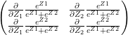
The 3 equations for the 2 layer Neural Network representation of Logistic Regression are
 -(a)
-(a)
 -(b)
-(b)
 -(c)
-(c)
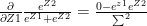
The back propagation step requires the computation of  and
and  . In the case of regression it would be
  and
and  where dE is the Mean Squared Error function.
Computing the derivatives for back propagation we have
 -(d)
-(d)
because 
Also from equation (2) we get
 – (e)
– (e)
By chain rule

therefore substituting the results of (d) & (e) we get
 (f)
(f)
Finally
 -(g)
-(g)
 – (h)
– (h)
and from (f) we have 
Therefore (g) reduces to
 -(i)
-(i)
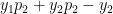
Also
 -(j)
-(j)
Since
 and using (f) in (j)

The gradient computes the weights at the input layer and the corresponding bias by using the values
of  and
and 


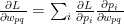
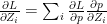
I found the computation graph representation in the book Deep Learning: Ian Goodfellow, Yoshua Bengio, Aaron Courville, very useful to visualize and also compute the backward propagation. For the 2 layer Neural Network of Logistic Regression the computation graph is shown below

3. Neural Network for Logistic Regression -Python code (vectorized)
import numpy as np
import pandas as pd
import os
import matplotlib.pyplot as plt
from sklearn.model_selection import train_test_split
def sigmoid(z):
a=1/(1+np.exp(-z))
return a
def initialize(dim):
w = np.zeros(dim).reshape(dim,1)
b = 0
return w
def computeLoss(numTraining,Y,A):
loss=-1/numTraining *np.sum(Y*np.log(A) + (1-Y)*(np.log(1-A)))
return(loss)
def forwardPropagation(w,b,X,Y):
Z=np.dot(w.T,X)+b
numTraining=float(len(X))
A=sigmoid(Z)
loss = computeLoss(numTraining,Y,A)
dZ=A-Y
dw=1/numTraining*np.dot(X,dZ.T)
db=1/numTraining*np.sum(dZ)
gradients = {"dw": dw,
"db": db}
loss = np.squeeze(loss)
return gradients,loss
def gradientDescent(w, b, X, Y, numIerations, learningRate):
losses=[]
idx =[]
for i in range(numIerations):
gradients,loss=forwardPropagation(w,b,X,Y)
dw = gradients["dw"]
db = gradients["db"]
w = w-learningRate*dw
b = b-learningRate*db
if i % 100 == 0:
idx.append(i)
losses.append(loss)
params = {"w": w,
"b": b}
grads = {"dw": dw,
"db": db}
return params, grads, losses,idx
def predict(w,b,X):
size=X.shape[1]
yPredicted=np.zeros((1,size))
Z=np.dot(w.T,X)
A=sigmoid(Z)
for i in range(A.shape[1]):
if(A[0][i] > 0.5):
yPredicted[0][i]=1
else:
yPredicted[0][i]=0
return yPredicted
def normalize(x):
x_norm = None
x_norm = np.linalg.norm(x,axis=1,keepdims=True)
x= x/x_norm
return x
from sklearn.datasets import load_breast_cancer
(X_cancer, y_cancer) = load_breast_cancer(return_X_y = True)
X_train, X_test, y_train, y_test = train_test_split(X_cancer, y_cancer,
random_state = 0)
X_train1=normalize(X_train)
w=np.zeros((X_train.shape[1],1))
b=0
X_train1=normalize(X_train)
X_train2=X_train1.T
y_train1=y_train.reshape(len(y_train),1)
y_train2=y_train1.T
parameters, grads, costs,idx = gradientDescent(w, b, X_train2, y_train2, numIerations=4000, learningRate=0.75)
w = parameters["w"]
b = parameters["b"]
X_test1=normalize(X_test)
X_test2=X_test1.T
y_test1=y_test.reshape(len(y_test),1)
y_test2=y_test1.T
yPredictionTest = predict(w, b, X_test2)
yPredictionTrain = predict(w, b, X_train2)
print("train accuracy: {} %".format(100 - np.mean(np.abs(yPredictionTrain - y_train2)) * 100))
print("test accuracy: {} %".format(100 - np.mean(np.abs(yPredictionTest - y_test)) * 100))
fig1=plt.plot(idx,costs)
fig1=plt.title("Gradient descent-Cost vs No of iterations")
fig1=plt.xlabel("No of iterations")
fig1=plt.ylabel("Cost")
fig1.figure.savefig("fig1", bbox_inches='tight')
## train accuracy: 90.3755868545 %
## test accuracy: 89.5104895105 %
Note: It can be seen that the Accuracy on the training and test set is 90.37% and 89.51%. This is comparatively poorer than the 96% which the logistic regression of sklearn achieves! But this is mainly because of the absence of hidden layers which is the real power of neural networks.

4. Neural Network for Logistic Regression -R code (vectorized)
source("RFunctions-1.R")
sigmoid <- function(z){
a <- 1/(1+ exp(-z))
a
}
computeLoss <- function(numTraining,Y,A){
loss <- -1/numTraining* sum(Y*log(A) + (1-Y)*log(1-A))
return(loss)
}
forwardPropagation <- function(w,b,X,Y){
Z <- t(w) %*% X +b
numTraining <- ncol(X)
A=sigmoid(Z)
loss <- computeLoss(numTraining,Y,A)
dZ<-A-Y
dw<-1/numTraining * X %*% t(dZ)
db<-1/numTraining*sum(dZ)
fwdProp <- list("loss" = loss, "dw" = dw, "db" = db)
return(fwdProp)
}
gradientDescent <- function(w, b, X, Y, numIerations, learningRate){
losses <- NULL
idx <- NULL
for(i in 1:numIerations){
fwdProp <-forwardPropagation(w,b,X,Y)
dw <- fwdProp$dw
db <- fwdProp$db
w = w-learningRate*dw
b = b-learningRate*db
l <- fwdProp$loss
if(i %% 100 == 0){
idx <- c(idx,i)
losses <- c(losses,l)
}
}
gradDescnt <- list("w"=w,"b"=b,"dw"=dw,"db"=db,"losses"=losses,"idx"=idx)
return(gradDescnt)
}
predict <- function(w,b,X){
m=dim(X)[2]
yPredicted=matrix(rep(0,m),nrow=1,ncol=m)
Z <- t(w) %*% X +b
A=sigmoid(Z)
for(i in 1:dim(A)[2]){
if(A[1,i] > 0.5)
yPredicted[1,i]=1
else
yPredicted[1,i]=0
}
return(yPredicted)
}
normalize <- function(x){
n<-as.matrix(sqrt(rowSums(x^2)))
normalized<-sweep(x, 1, n, FUN="/")
return(normalized)
}
cancer <- read.csv("cancer.csv")
names(cancer) <- c(seq(1,30),"output")
train_idx <- trainTestSplit(cancer,trainPercent=75,seed=5)
train <- cancer[train_idx, ]
test <- cancer[-train_idx, ]
X_train <-train[,1:30]
y_train <- train[,31]
X_test <- test[,1:30]
y_test <- test[,31]
w <-matrix(rep(0,dim(X_train)[2]))
b <-0
X_train1 <- normalize(X_train)
X_train2=t(X_train1)
y_train1=as.matrix(y_train)
y_train2=t(y_train1)
gradDescent= gradientDescent(w, b, X_train2, y_train2, numIerations=3000, learningRate=0.77)
X_test1=normalize(X_test)
X_test2=t(X_test1)
y_test1=as.matrix(y_test)
y_test2=t(y_test1)
yPredictionTest = predict(gradDescent$w, gradDescent$b, X_test2)
yPredictionTrain = predict(gradDescent$w, gradDescent$b, X_train2)
sprintf("Train accuracy: %f",(100 - mean(abs(yPredictionTrain - y_train2)) * 100))
## [1] "Train accuracy: 90.845070"
sprintf("test accuracy: %f",(100 - mean(abs(yPredictionTest - y_test)) * 100))
## [1] "test accuracy: 87.323944"
df <-data.frame(gradDescent$idx, gradDescent$losses)
names(df) <- c("iterations","losses")
ggplot(df,aes(x=iterations,y=losses)) + geom_point() + geom_line(col="blue") +
    ggtitle("Gradient Descent - Losses vs No of Iterations") +
    xlab("No of iterations") + ylab("Losses")

4. Neural Network for Logistic Regression -Octave code (vectorized)
1;

# Define sigmoid function

function a = sigmoid(z)

a = 1 ./ (1+ exp(-z));

end

# Compute the loss

function loss=computeLoss(numtraining,Y,A)

loss = -1/numtraining * sum((Y .* log(A)) + (1-Y) .* log(1-A));

end
# Perform forward propagation

function [loss,dw,db,dZ] = forwardPropagation(w,b,X,Y)

% Compute Z

Z = w' * X + b;

numtraining = size(X)(1,2);

# Compute sigmoid

A = sigmoid(Z);
#Compute loss. Note this is element wise product

loss =computeLoss(numtraining,Y,A);

# Compute the gradients dZ, dw and db

dZ = A-Y;

dw = 1/numtraining* X * dZ';

db =1/numtraining*sum(dZ);
end
# Compute Gradient Descent

function [w,b,dw,db,losses,index]=gradientDescent(w, b, X, Y, numIerations, learningRate)

#Initialize losses and idx

losses=[];

index=[];

# Loop through the number of iterations

for i=1:numIerations,

[loss,dw,db,dZ] = forwardPropagation(w,b,X,Y);

# Perform Gradient descent

w = w - learningRate*dw;

b = b - learningRate*db;

if(mod(i,100) ==0)

# Append index and loss

index = [index i];

losses = [losses loss];

endif
end
end
# Determine the predicted value for dataset

function yPredicted = predict(w,b,X)

m = size(X)(1,2);

yPredicted=zeros(1,m);

# Compute Z

Z = w' * X + b;

# Compute sigmoid

A = sigmoid(Z);

for i=1:size(X)(1,2),

# Set predicted as 1 if A > 0,5

if(A(1,i) >= 0.5)

yPredicted(1,i)=1;

else

yPredicted(1,i)=0;

endif

end

end
# Normalize by dividing each value by the sum of squares

function normalized = normalize(x)

# Compute Frobenius norm. Square the elements, sum rows and then find square root

a = sqrt(sum(x .^ 2,2));

# Perform element wise division

normalized = x ./ a;

end
# Split into train and test sets

function [X_train,y_train,X_test,y_test] = trainTestSplit(dataset,trainPercent)

# Create a random index

ix = randperm(length(dataset));

# Split into training

trainSize = floor(trainPercent/100 * length(dataset));

train=dataset(ix(1:trainSize),:);

# And test

test=dataset(ix(trainSize+1:length(dataset)),:);

X_train = train(:,1:30);

y_train = train(:,31);

X_test = test(:,1:30);

y_test = test(:,31);

end
cancer=csvread("cancer.csv");

[X_train,y_train,X_test,y_test] = trainTestSplit(cancer,75);

w=zeros(size(X_train)(1,2),1);

b=0;

X_train1=normalize(X_train);

X_train2=X_train1';

y_train1=y_train';

[w1,b1,dw,db,losses,idx]=gradientDescent(w, b, X_train2, y_train1, numIerations=3000, learningRate=0.75);

# Normalize X_test

X_test1=normalize(X_test);

#Transpose X_train so that we have a matrix as (features, numSamples)

X_test2=X_test1';

y_test1=y_test';

# Use the values of the weights generated from Gradient Descent

yPredictionTest = predict(w1, b1, X_test2);

yPredictionTrain = predict(w1, b1, X_train2);
trainAccuracy=100-mean(abs(yPredictionTrain - y_train1))*100

testAccuracy=100- mean(abs(yPredictionTest - y_test1))*100

trainAccuracy =  90.845

testAccuracy =  89.510

graphics_toolkit('gnuplot')

plot(idx,losses);

title ('Gradient descent- Cost vs No of iterations');

xlabel ("No of iterations");

ylabel ("Cost");

Conclusion
This post starts with a simple 2 layer Neural Network implementation of Logistic Regression. Clearly the performance of this simple Neural Network is comparatively poor to the highly optimized sklearn’s Logistic Regression. This is because the above neural network did not have any hidden layers. Deep Learning & Neural Networks achieve extraordinary performance because of the presence of deep hidden layers
The Deep Learning journey has begun… Don’t miss the bus!
Stay tuned for more interesting posts in Deep Learning!!
References
1. Deep Learning Specialization
2. Neural Networks for Machine Learning
3. Deep Learning, Ian Goodfellow, Yoshua Bengio and Aaron Courville
4. Neural Networks: The mechanics of backpropagation
5. Machine Learning
Also see
1. My book ‘Practical Machine Learning with R and Python’ on Amazon
2. Simplifying Machine Learning: Bias, Variance, regularization and odd facts – Part 4
3. The 3rd paperback & kindle editions of my books on Cricket, now on Amazon
4. Practical Machine Learning with R and Python – Part 4
5. Introducing QCSimulator: A 5-qubit quantum computing simulator in R
6. A Bluemix recipe with MongoDB and Node.js
7. My travels through the realms of Data Science, Machine Learning, Deep Learning and (AI)
To see all posts check Index of posts

 In this book I implement some of the most common, but important Machine Learning algorithms in R and equivalent Python code.


 – (A)
– (A)


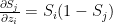 when i=j
 when
when 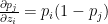 when i=j

 when i=j and 0 when


 (1)
(1) (2)
(2)


 when i=j
 when
when 


 which similarly reduces to


 and
and 
 and
and 


