Introducing cricket package yorkr:Part 4-In the block hole!

Introduction

“The nitrogen in our DNA, the calcium in our teeth, the iron in our blood, the carbon in our apple pies were made in the interiors of collapsing stars. We are made of starstuff.”

“If you wish to make an apple pie from scratch, you must first invent the universe.”

“We are like butterflies who flutter for a day and think it is forever.”

“The absence of evidence is not the evidence of absence.”

“We are star stuff which has taken its destiny into its own hands.”

                              Cosmos - Carl Sagan

This post is the 4th and possibly, the last part of my introduction, to my latest cricket package yorkr. This is the 4th part of the introduction, the 3 earlier ones were

  1. Introducing cricket package yorkr-Part1:Beaten by sheer pace!.
  2. Introducing cricket package yorkr: Part 2-Trapped leg before wicket!
  3. Introducing cricket package yorkr: Part 3-Foxed by flight!

The 1st part included functions dealing with a specific match, the 2nd part dealt with functions between 2 opposing teams. The 3rd part dealt with functions between a team and all matches with all oppositions. This 4th part includes individual batting and bowling performances in ODI matches and deals with Class 4 functions.

If you are passionate about cricket, and love analyzing cricket performances, then check out my 2 racy books on cricket! In my books, I perform detailed yet compact analysis of performances of both batsmen, bowlers besides evaluating team & match performances in Tests , ODIs, T20s & IPL. You can buy my books on cricket from Amazon at $12.99 for the paperback and $4.99/$6.99 respectively for the kindle versions. The books can be accessed at Cricket analytics with cricketr  and Beaten by sheer pace-Cricket analytics with yorkr  A must read for any cricket lover! Check it out!!

1

d $4.99/Rs 320 and $6.99/Rs448 respectively


This post has also been published at RPubs yorkr-Part4 and can also be downloaded as a PDF document from yorkr-Part4.pdf.

You can clone/fork the code for the package yorkr from Github at yorkr-package

Checkout my interactive Shiny apps GooglyPlus (plots & tables) and Googly (only plots) which can be used to analyze IPL players, teams and matches.

Important note 1: Do check out all the posts on the python avatar of yorkr, namely ‘yorkpy’ in my post ‘Pitching yorkpy … short of good length to IPL – Part 1

Batsman functions

  1. batsmanRunsVsDeliveries
  2. batsmanFoursSixes
  3. batsmanDismissals
  4. batsmanRunsVsStrikeRate
  5. batsmanMovingAverage
  6. batsmanCumulativeAverageRuns
  7. batsmanCumulativeStrikeRate
  8. batsmanRunsAgainstOpposition
  9. batsmanRunsVenue
  10. batsmanRunsPredict

Bowler functions

  1. bowlerMeanEconomyRate
  2. bowlerMeanRunsConceded
  3. bowlerMovingAverage
  4. bowlerCumulativeAvgWickets
  5. bowlerCumulativeAvgEconRate
  6. bowlerWicketPlot
  7. bowlerWicketsAgainstOpposition
  8. bowlerWicketsVenue
  9. bowlerWktsPredict

Note: The yorkr package in its current avatar only supports ODI, T20 and IPL T20 matches.

library(yorkr)
library(gridExtra)
library(rpart.plot)
library(dplyr)
library(ggplot2)
rm(list=ls())

A. Batsman functions

1. Get Team Batting details

The function below gets the overall team batting details based on the RData file available in ODI matches. This is currently also available in Github at (https://github.com/tvganesh/yorkrData/tree/master/ODI/ODI-matches).  However you may have to do this as future matches are added! The batting details of the team in each match is created and a huge data frame is created by rbinding the individual dataframes. This can be saved as a RData file

setwd("C:/software/cricket-package/york-test/yorkrData/ODI/ODI-matches")
india_details <- getTeamBattingDetails("India",dir=".", save=TRUE)
dim(india_details)
## [1] 11085    15
sa_details <- getTeamBattingDetails("South Africa",dir=".",save=TRUE)
dim(sa_details)
## [1] 6375   15
nz_details <- getTeamBattingDetails("New Zealand",dir=".",save=TRUE)
dim(nz_details)
## [1] 6262   15
eng_details <- getTeamBattingDetails("England",dir=".",save=TRUE)
dim(eng_details)
## [1] 9001   15

2. Get batsman details

This function is used to get the individual batting record for a the specified batsmen of the country as in the functions below. For analyzing the batting performances the following cricketers have been chosen

  1. Virat Kohli (Ind)
  2. M S Dhoni (Ind)
  3. AB De Villiers (SA)
  4. Q De Kock (SA)
  5. J Root (Eng)
  6. M J Guptill (NZ)
setwd("C:/software/cricket-package/york-test/yorkrData/ODI/ODI-matches")
kohli <- getBatsmanDetails(team="India",name="Kohli",dir=".")
## [1] "./India-BattingDetails.RData"
dhoni <- getBatsmanDetails(team="India",name="Dhoni")
## [1] "./India-BattingDetails.RData"
devilliers <-  getBatsmanDetails(team="South Africa",name="Villiers",dir=".")
## [1] "./South Africa-BattingDetails.RData"
deKock <-  getBatsmanDetails(team="South Africa",name="Kock",dir=".")
## [1] "./South Africa-BattingDetails.RData"
root <-  getBatsmanDetails(team="England",name="Root",dir=".")
## [1] "./England-BattingDetails.RData"
guptill <-  getBatsmanDetails(team="New Zealand",name="Guptill",dir=".")
## [1] "./New Zealand-BattingDetails.RData"

3. Runs versus deliveries

Kohli, De Villiers and Guptill have a good cluster of points that head towards 150 runs at 150 deliveries.

p1 <-batsmanRunsVsDeliveries(kohli,"Kohli")
p2 <- batsmanRunsVsDeliveries(dhoni, "Dhoni")
p3 <- batsmanRunsVsDeliveries(devilliers,"De Villiers")
p4 <- batsmanRunsVsDeliveries(deKock,"Q de Kock")
p5 <- batsmanRunsVsDeliveries(root,"JE Root")
p6 <- batsmanRunsVsDeliveries(guptill,"MJ Guptill")
grid.arrange(p1,p2,p3,p4,p5,p6, ncol=3)

runsVsDeliveries-1

4. Batsman Total runs, Fours and Sixes

The plots below show the total runs, fours and sixes by the batsmen

kohli46 <- select(kohli,batsman,ballsPlayed,fours,sixes,runs)
p1 <- batsmanFoursSixes(kohli46,"Kohli")
dhoni46 <- select(dhoni,batsman,ballsPlayed,fours,sixes,runs)
p2 <- batsmanFoursSixes(dhoni46,"Dhoni")
devilliers46 <- select(devilliers,batsman,ballsPlayed,fours,sixes,runs)
p3 <- batsmanFoursSixes(devilliers46, "De Villiers")
deKock46 <- select(deKock,batsman,ballsPlayed,fours,sixes,runs)
p4 <- batsmanFoursSixes(deKock46,"Q de Kock")
root46 <- select(root,batsman,ballsPlayed,fours,sixes,runs)
p5 <- batsmanFoursSixes(root46,"JE Root")
guptill46 <- select(guptill,batsman,ballsPlayed,fours,sixes,runs)
p6 <- batsmanFoursSixes(guptill46,"MJ Guptill")
grid.arrange(p1,p2,p3,p4,p5,p6, ncol=3)

foursSixes-1

5. Batsman dismissals

The type of dismissal for each batsman is shown below

p1 <-batsmanDismissals(kohli,"Kohli")
p2 <- batsmanDismissals(dhoni, "Dhoni")
p3 <- batsmanDismissals(devilliers, "De Villiers")
p4 <- batsmanDismissals(deKock,"Q de Kock")
p5 <- batsmanDismissals(root,"JE Root")
p6 <- batsmanDismissals(guptill,"MJ Guptill")
grid.arrange(p1,p2,p3,p4,p5,p6, ncol=3)

dismissal-1

6. Runs versus Strike Rate

De villiers has the best strike rate among all as there are more points to the right side of the plot for the same runs. Kohli and Dhoni do well too. Q De Kock and Joe Root also have a very good spread of points though they have fewer innings.

p1 <-batsmanRunsVsStrikeRate(kohli,"Kohli")
p2 <- batsmanRunsVsStrikeRate(dhoni, "Dhoni")
p3 <- batsmanRunsVsStrikeRate(devilliers, "De Villiers")
p4 <- batsmanRunsVsStrikeRate(deKock,"Q de Kock")
p5 <- batsmanRunsVsStrikeRate(root,"JE Root")
p6 <- batsmanRunsVsStrikeRate(guptill,"MJ Guptill")
grid.arrange(p1,p2,p3,p4,p5,p6, ncol=3)

runsSR-1

7. Batsman moving average

Kohli’s average is on a gentle increase from below 50 to around 60’s. Joe Root performance is impressive with his moving average of late tending towards the 70’s. Q De Kock seemed to have a slump around 2015 but his performance is on the increase. Devilliers consistently averages around 50. Dhoni also has been having a stable run in the last several years.

p1 <-batsmanMovingAverage(kohli,"Kohli")
p2 <- batsmanMovingAverage(dhoni, "Dhoni")
p3 <- batsmanMovingAverage(devilliers, "De Villiers")
p4 <- batsmanMovingAverage(deKock,"Q de Kock")
p5 <- batsmanMovingAverage(root,"JE Root")
p6 <- batsmanMovingAverage(guptill,"MJ Guptill")
grid.arrange(p1,p2,p3,p4,p5,p6, ncol=3)

ma-1

8. Batsman cumulative average

The functions below provide the cumulative average of runs scored. As can be seen Kohli and Devilliers have a cumulative runs rate that averages around 48-50. Q De Kock seems to have had a rocky career with several highs and lows as the cumulative average oscillates between 45-40. Root steadily improves to a cumulative average of around 42-43 from his 50th innings

p1 <-batsmanCumulativeAverageRuns(kohli,"Kohli")
p2 <- batsmanCumulativeAverageRuns(dhoni, "Dhoni")
p3 <- batsmanCumulativeAverageRuns(devilliers, "De Villiers")
p4 <- batsmanCumulativeAverageRuns(deKock,"Q de Kock")
p5 <- batsmanCumulativeAverageRuns(root,"JE Root")
p6 <- batsmanCumulativeAverageRuns(guptill,"MJ Guptill")
grid.arrange(p1,p2,p3,p4,p5,p6, ncol=3)

cAvg-1

9. Cumulative Average Strike Rate

The plots below show the cumulative average strike rate of the batsmen. Dhoni and Devilliers have the best cumulative average strike rate of 90%. The rest average around 80% strike rate. Guptill shows a slump towards the latter part of his career.

p1 <-batsmanCumulativeStrikeRate(kohli,"Kohli")
p2 <- batsmanCumulativeStrikeRate(dhoni, "Dhoni")
p3 <- batsmanCumulativeStrikeRate(devilliers, "De Villiers")
p4 <- batsmanCumulativeStrikeRate(deKock,"Q de Kock")
p5 <- batsmanCumulativeStrikeRate(root,"JE Root")
p6 <- batsmanCumulativeStrikeRate(guptill,"MJ Guptill")
grid.arrange(p1,p2,p3,p4,p5,p6, ncol=3)

cSR-1

10. Batsman runs against opposition

Kohli’s best performances are against Australia, West Indies and Sri Lanka

batsmanRunsAgainstOpposition(kohli,"Kohli")

runsOppn1-1

batsmanRunsAgainstOpposition(dhoni, "Dhoni")

runsOppn2-1

Kohli’s best performances are against Australia, Pakistan and West Indies

batsmanRunsAgainstOpposition(devilliers, "De Villiers")

runsOppn3-1

Quentin de Kock average almost 100 runs against India and 75 runs against England

batsmanRunsAgainstOpposition(deKock, "Q de Kock")

runsOppn4-1

Root’s best performances are against South Africa, Sri Lanka and West Indies

batsmanRunsAgainstOpposition(root, "JE Root")

runsOppn5-1

batsmanRunsAgainstOpposition(guptill, "MJ Guptill")

runsOppn6-1

11. Runs at different venues

The plots below give the performances of the batsmen at different grounds.

batsmanRunsVenue(kohli,"Kohli")

runsVenue1-1

batsmanRunsVenue(dhoni, "Dhoni")

runsVenue2-1

batsmanRunsVenue(devilliers, "De Villiers")

runsVenue3-1

batsmanRunsVenue(deKock, "Q de Kock")

runsVenue4-1

batsmanRunsVenue(root, "JE Root")

runsVenue5-1

batsmanRunsVenue(guptill, "MJ Guptill")

runsVenue6-1

12. Predict number of runs to deliveries

The plots below use rpart classification tree to predict the number of deliveries required to score the runs in the leaf node. For e.g. Kohli takes 66 deliveries to score 64 runs and for higher number of deliveries scores around 115 runs. Devilliers needs

par(mfrow=c(1,3))
par(mar=c(4,4,2,2))
batsmanRunsPredict(kohli,"Kohli")
batsmanRunsPredict(dhoni, "Dhoni")
batsmanRunsPredict(devilliers, "De Villiers")

runsPredict1,runsVenue1-1

par(mfrow=c(1,3))
par(mar=c(4,4,2,2))
batsmanRunsPredict(deKock,"Q de Kock")
batsmanRunsPredict(root,"JE Root")
batsmanRunsPredict(guptill,"MJ Guptill")

runsPredict2,runsVenue1-1

B. Bowler functions

13. Get bowling details

The function below gets the overall team bowling details based on the RData file available in ODI matches. This is currently also available in Github at (https://github.com/tvganesh/yorkrData/tree/master/ODI/ODI-matches). The bowling details of the team in each match is created and a huge data frame is created by rbinding the individual dataframes. This can be saved as a RData file

setwd("C:/software/cricket-package/york-test/yorkrData/ODI/ODI-matches")
ind_bowling <- getTeamBowlingDetails("India",dir=".",save=TRUE)
dim(ind_bowling)
## [1] 7816   12
aus_bowling <- getTeamBowlingDetails("Australia",dir=".",save=TRUE)
dim(aus_bowling)
## [1] 9191   12
ban_bowling <- getTeamBowlingDetails("Bangladesh",dir=".",save=TRUE)
dim(ban_bowling)
## [1] 5665   12
sa_bowling <- getTeamBowlingDetails("South Africa",dir=".",save=TRUE)
dim(sa_bowling)
## [1] 3806   12
sl_bowling <- getTeamBowlingDetails("Sri Lanka",dir=".",save=TRUE)
dim(sl_bowling)
## [1] 3964   12

14. Get bowling details of the individual bowlers

This function is used to get the individual bowling record for a specified bowler of the country as in the functions below. For analyzing the bowling performances the following cricketers have been chosen

  1. R A Jadeja (Ind)
  2. Ravichander Ashwin (Ind)
  3. Mitchell Starc (Aus)
  4. Shakib Al Hasan (Ban)
  5. Ajantha Mendis (SL)
  6. Dale Steyn (SA)
jadeja <- getBowlerWicketDetails(team="India",name="Jadeja",dir=".")
ashwin <- getBowlerWicketDetails(team="India",name="Ashwin",dir=".")
starc <-  getBowlerWicketDetails(team="Australia",name="Starc",dir=".")
shakib <-  getBowlerWicketDetails(team="Bangladesh",name="Shakib",dir=".")
mendis <-  getBowlerWicketDetails(team="Sri Lanka",name="Mendis",dir=".")
steyn <-  getBowlerWicketDetails(team="South Africa",name="Steyn",dir=".")

15. Bowler Mean Economy Rate

Shakib Al Hassan is expensive in the 1st 3 overs after which he is very economical with a economy rate of 3-4. Starc, Steyn average around a ER of 4.0

p1<-bowlerMeanEconomyRate(jadeja,"RA Jadeja")
p2<-bowlerMeanEconomyRate(ashwin, "R Ashwin")
p3<-bowlerMeanEconomyRate(starc, "MA Starc")
p4<-bowlerMeanEconomyRate(shakib, "Shakib Al Hasan")
p5<-bowlerMeanEconomyRate(mendis, "A Mendis")
p6<-bowlerMeanEconomyRate(steyn, "D Steyn")
grid.arrange(p1,p2,p3,p4,p5,p6, ncol=3)

meanER-1

16. Bowler Mean Runs conceded

Ashwin is expensive around 6 & 7 overs

p1<-bowlerMeanRunsConceded(jadeja,"RA Jadeja")
p2<-bowlerMeanRunsConceded(ashwin, "R Ashwin")
p3<-bowlerMeanRunsConceded(starc, "M A Starc")
p4<-bowlerMeanRunsConceded(shakib, "Shakib Al Hasan")
p5<-bowlerMeanRunsConceded(mendis, "A Mendis")
p6<-bowlerMeanRunsConceded(steyn, "D Steyn")
grid.arrange(p1,p2,p3,p4,p5,p6, ncol=3)

meanRunsConceded-1

17. Bowler Moving average

RA jadeja and Mendis’ performance has dipped considerably, while Ashwin and Shakib have improving performances. Starc average around 4 wickets

p1<-bowlerMovingAverage(jadeja,"RA Jadeja")
p2<-bowlerMovingAverage(ashwin, "Ashwin")
p3<-bowlerMovingAverage(starc, "M A Starc")
p4<-bowlerMovingAverage(shakib, "Shakib Al Hasan")
p5<-bowlerMovingAverage(mendis, "Ajantha Mendis")
p6<-bowlerMovingAverage(steyn, "Dale Steyn")
grid.arrange(p1,p2,p3,p4,p5,p6, ncol=3)

bowlerMA-1

17. Bowler cumulative average wickets

Starc is clearly the most consistent performer with 3 wickets on an average over his career, while Jadeja averages around 2.0. Ashwin seems to have dropped from 2.4-2.0 wickets, while Mendis drops from high 3.5 to 2.2 wickets. The fractional wickets only show a tendency to take another wicket.

p1<-bowlerCumulativeAvgWickets(jadeja,"RA Jadeja")
p2<-bowlerCumulativeAvgWickets(ashwin, "Ashwin")
p3<-bowlerCumulativeAvgWickets(starc, "M A Starc")
p4<-bowlerCumulativeAvgWickets(shakib, "Shakib Al Hasan")
p5<-bowlerCumulativeAvgWickets(mendis, "Ajantha Mendis")
p6<-bowlerCumulativeAvgWickets(steyn, "Dale Steyn")
grid.arrange(p1,p2,p3,p4,p5,p6, ncol=3)

cumWkts-1

18. Bowler cumulative Economy Rate (ER)

The plots below are interesting. All of the bowlers seem to average around 4.5 runs/over. RA Jadeja’s ER improves and heads to 4.5, Mendis is seen to getting more expensive as his career progresses. From a ER of 3.0 he increases towards 4.5

p1<-bowlerCumulativeAvgEconRate(jadeja,"RA Jadeja")
p2<-bowlerCumulativeAvgEconRate(ashwin, "Ashwin")
p3<-bowlerCumulativeAvgEconRate(starc, "M A Starc")
p4<-bowlerCumulativeAvgEconRate(shakib, "Shakib Al Hasan")
p5<-bowlerCumulativeAvgEconRate(mendis, "Ajantha Mendis")
p6<-bowlerCumulativeAvgEconRate(steyn, "Dale Steyn")
grid.arrange(p1,p2,p3,p4,p5,p6, ncol=3)

cumER-1

19. Bowler wicket plot

The plot below gives the average wickets versus number of overs

p1<-bowlerWicketPlot(jadeja,"RA Jadeja")
p2<-bowlerWicketPlot(ashwin, "Ashwin")
p3<-bowlerWicketPlot(starc, "M A Starc")
p4<-bowlerWicketPlot(shakib, "Shakib Al Hasan")
p5<-bowlerWicketPlot(mendis, "Ajantha Mendis")
p6<-bowlerWicketPlot(steyn, "Dale Steyn")
grid.arrange(p1,p2,p3,p4,p5,p6, ncol=3)

wktPlot-1

20. Bowler wicket against opposition

#Jadeja's' best pertformance are against England, Pakistan and West Indies
bowlerWicketsAgainstOpposition(jadeja,"RA Jadeja")

wktsOppn1-1

#Ashwin's bets pertformance are against England, Pakistan and South Africa
bowlerWicketsAgainstOpposition(ashwin, "Ashwin")

wktsOppn2-1

#Starc has good performances against India, New Zealand, Pakistan, West Indies
bowlerWicketsAgainstOpposition(starc, "M A Starc")

wktsOppn3-1

bowlerWicketsAgainstOpposition(shakib,"Shakib Al Hasan")

wktsOppn4-1

bowlerWicketsAgainstOpposition(mendis, "Ajantha Mendis")

wktsOppn5-1

#Steyn has good performances against India, Sri Lanka, Pakistan, West Indies
bowlerWicketsAgainstOpposition(steyn, "Dale Steyn")

wktsOppn6-1

21. Bowler wicket at cricket grounds

bowlerWicketsVenue(jadeja,"RA Jadeja")

wktsAve1-1

bowlerWicketsVenue(ashwin, "Ashwin")

wktsAve2-1

bowlerWicketsVenue(starc, "M A Starc")
## Warning: Removed 2 rows containing missing values (geom_bar).

wktsAve3-1

bowlerWicketsVenue(shakib,"Shakib Al Hasan")

wktsAve4-1

bowlerWicketsVenue(mendis, "Ajantha Mendis")

wktsAve5-1

bowlerWicketsVenue(steyn, "Dale Steyn")

wktsAve6-1

22. Get Delivery wickets for bowlers

Thsi function creates a dataframe of deliveries and the wickets taken

setwd("C:/software/cricket-package/york-test/yorkrData/ODI/ODI-matches")
jadeja1 <- getDeliveryWickets(team="India",dir=".",name="Jadeja",save=FALSE)
ashwin1 <- getDeliveryWickets(team="India",dir=".",name="Ashwin",save=FALSE)
starc1 <- getDeliveryWickets(team="Australia",dir=".",name="MA Starc",save=FALSE)
shakib1 <- getDeliveryWickets(team="Bangladesh",dir=".",name="Shakib",save=FALSE)
mendis1 <- getDeliveryWickets(team="Sri Lanka",dir=".",name="Mendis",save=FALSE)
steyn1 <- getDeliveryWickets(team="South Africa",dir=".",name="Steyn",save=FALSE)

23. Predict number of deliveries to wickets

#Jadeja and Ashwin need around 22 to 28 deliveries to make a break through
par(mfrow=c(1,2))
par(mar=c(4,4,2,2))
bowlerWktsPredict(jadeja1,"RA Jadeja")
bowlerWktsPredict(ashwin1,"RAshwin")

wktsPred1-1

#Starc and Shakib provide an early breakthrough producing a wicket in around 16 balls. Starc's 2nd wicket comed around the 30th delivery
par(mfrow=c(1,2))
par(mar=c(4,4,2,2))
bowlerWktsPredict(starc1,"MA Starc")
bowlerWktsPredict(shakib1,"Shakib Al Hasan")

wktsPred2-1

#Steyn and Mendis take 20 deliveries to get their 1st wicket
par(mfrow=c(1,2))
par(mar=c(4,4,2,2))
bowlerWktsPredict(mendis1,"A Mendis")
bowlerWktsPredict(steyn1,"DSteyn")

wktsPred3-1

Conclusion

This concludes the 4 part introduction to my new R cricket package yorkr for ODIs. I will be enhancing the package to handle Twenty20 and IPL matches soon. You can fork/clone the code from Github at yorkr.

The yaml data from Cricsheet have already beeen converted into R consumable dataframes. The converted data can be downloaded from Github at yorkrData. There are 3 folders – ODI matches, ODI matches between 2 teams (oppnAllMatches), ODI matches between a team and the rest of the world (all matches,all oppositions).

As I have already mentioned I have around 67 functions for analysis, however I am certain that the data has a lot more secrets waiting to be tapped. So please do go ahead and run any machine learning or statistical learning algorithms on them. If you do come up with interesting insights, I would appreciate if attribute the source to Cricsheet(http://cricsheet.org), and my package yorkr and my blog Giga thoughts*, besides dropping me a note.

Hope you have a great time with my yorkr package!

Important note: Do check out my other posts using yorkr at yorkr-posts

Also see

  1. Introducing cricketr! : An R package to analyze performances of cricketers
  2. Cricket analytics with cricketr in paperback and Kindle versions
  3. My TEDx talk on the “Internet of Things”
  4. Bend it like Bluemix,MongoDB with autoscaling – Part 1
  5. The mind of a programmer
  6. Fun simulation of a chain in Android
  7. Taking cricketr for a spin-Part 1
  8. Latency,throughput implications for the cloud
  9. Hand detection through haar-training: A hands-on approach
  10. Cricket analytics with cricketr

Introducing cricket package yorkr: Part 3-Foxed by flight!

Introduction

He will win, who knows when to fight and when not to fight.

He will win, who knows how to handle both superior and inferior forces

If you know neither the enemy nor yourself, you will succumb in every battle.

Hence the skilful fighter puts himself in a position which makes defeat impossible, and does not miss the moment for defeating the enemy.

Hence that general is skillful in attack whose opponent does not know what to defend; and he is skilled in defense whose opponent does know what to attack.

                                         The Art of War - Sun Tzu

This post is a continuation of my introduction to my latest cricket package yorkr. This is the 3rd part of the introduction, the 2 earlier ones were

  1. Introducing cricket package yorkr-Part1:Beaten by sheer pace!.
  2. Introducing cricket package yorkr: Part 2-Trapped leg before wicket!

This post deals with Class 3 functions, namely the performances of a team in all matches against all oppositions for e.g India/Australia/South Africa against all oppositions in all matches. In other words it is the performance of the team against the rest of the world.

If you are passionate about cricket, and love analyzing cricket performances, then check out my 2 racy books on cricket! In my books, I perform detailed yet compact analysis of performances of both batsmen, bowlers besides evaluating team & match performances in Tests , ODIs, T20s & IPL. You can buy my books on cricket from Amazon at $12.99 for the paperback and $4.99/$6.99 respectively for the kindle versions. The books can be accessed at Cricket analytics with cricketr  and Beaten by sheer pace-Cricket analytics with yorkr  A must read for any cricket lover! Check it out!!

1


This post has also been published at RPubs yorkr-Part3 and can also be downloaded as a PDF document from yorkr-Part3.pdf.

You can clone/fork the code for the package yorkr from Github at yorkr-package

Checkout my interactive Shiny apps GooglyPlus (plots & tables) and Googly (only plots) which can be used to analyze IPL players, teams and matches.

Important note 1: Do check out all the posts on the python avatar of yorkr, namely ‘yorkpy’ in my post ‘Pitching yorkpy … short of good length to IPL – Part 1

The list of functions in Class 3 are

  1. teamBattingScorecardAllOppnAllMatches()
  2. teamBatsmenPartnershipAllOppnAllMatches()
  3. teamBatsmenPartnershipAllOppnAllMatchesPlot()
  4. teamBatsmenVsBowlersAllOppnAllMatchesRept()
  5. teamBatsmenVsBowlersAllOppnAllMatchesPlot()
  6. teamBowlingScorecardAllOppnAllMatchesMain()
  7. teamBowlersVsBatsmenAllOppnAllMatchesRept()
  8. teamBowlersVsBatsmenAllOppnAllMatchesPlot()
  9. teamBowlingWicketKindAllOppnAllMatches()
  10. teamBowlingWicketRunsAllOppnAllMatches()

Note 1: The yorkr package in its current avatar supports ODI, T20 and IPL T20 matches. 

Note 2: As in the previous parts the plots usually have the plot=TRUE/FALSE parameter. This is to allow the user to get a return value of the desired dataframe. The user can choose to plot this, in any way he/she likes for e.g in interactive charts using rcharts, ggvis,googleVis,plotly etc

1. Install the package from CRAN

The yorkr package can be installed directly from CRAN now! Install the yorkr package.

if (!require("yorkr")) {
  install.packages("yorkr") 
  library("yorkr")
}
rm(list=ls())

2. Get data for all matches against all oppositions for a team

We can get all matches against all oppositions for a team/country using the function below. The dir parameter should point to the folder in which the RData files of the individual matches exist. This function creates a data frame of all the matches and also saves the resulting dataframe as RData

setwd("C:/software/cricket-package/york-test/yorkrData/ODI/ODI-team-allmatches-allOppositions")

# Get all matches against all oppositions for India and save as RData
matches <-getAllMatchesAllOpposition("India",dir=".",save=TRUE)
dim(matches)
## [1] 140655     25

“`

3. Save data for all matches against all oppositions

This can be done locally using the function below. This function gets all the matches of the country/team against all other countrioes//teams and combines them into a single dataframe and saves it in the current folder. The current implementation expects that the the RData files of individual matches are in ../data folder. Since I already have converted this I will not be running this again

#saveAllMatchesAllOpposition(dir=".",odir=".")

4. Load data directly for all matches between 2 teams

As in my earlier posts (yorkr-Part1 & yorkr-Part2) I have however already saved the data, for all matches of the individual countries, against all oppositons. The data for these matches for the individual teams/countries can be downloaded directly from Github folder at ODI-team-allmatches-allOppositions

Note: The dataframe for the different for all the matches of a country agaisnt all oppositons can be loaded directly into your code. As can be seen in the calls below the datframes are ~100,000+ rows x 25 columns. While I have 10+ functions to process these dataframes, for a particular team, feel free to download these data frames and perform your own analysis. The data frames include ball-by-ball details, details on non-striker, bowler, runs, extras, venue,date etc. Certainly these data frames are a gold-mine of interesting insights. So do go ahead and unleash your bagging/boosting algorithms, SVM classifiers or Random Forest algorithm on them.

I plan to try out some algorithms of statistical/machine learning in the months to come. If you do come up with interesting insights, I would appreciate if attribute the source to Cricsheet(http://cricsheet.org), and my package yorkr and my blog Giga thoughts, besides dropping me a note.*

As in my earlier post I will be directly loading the saved files. For the illustration of the functions, I will use India in all the functions, (for obvious reasons) and will randomly use the data from the rest of the top 8 teams

setwd("C:/software/cricket-package/york-test/yorkrData/ODI/ODI-team-allmatches-allOppositions")
load("allMatchesAllOpposition-India.RData")
ind_matches <- matches
dim(ind_matches)
## [1] 140655     25
load("allMatchesAllOpposition-Australia.RData")
aus_matches <- matches
dim(aus_matches)
## [1] 128148     25
load("allMatchesAllOpposition-New Zealand.RData")
nz_matches <- matches
dim(nz_matches)
## [1] 98573    25
load("allMatchesAllOpposition-Pakistan.RData")
pak_matches <- matches
dim(pak_matches)
## [1] 117947     25
load("allMatchesAllOpposition-England.RData")
eng_matches <- matches
dim(eng_matches)
## [1] 118859     25
load("allMatchesAllOpposition-Sri Lanka.RData")
sl_matches <- matches
dim(sl_matches)
## [1] 125893     25
load("allMatchesAllOpposition-West Indies.RData")
wi_matches <- matches
dim(wi_matches)
## [1] 92716    25
load("allMatchesAllOpposition-South Africa.RData")
sa_matches <- matches
dim(sa_matches)
## [1] 100916     25

5. Team Batting Scorecard (all matches with opposition)

The following functions shows the batting scorecards in each country. It returns a dataframe with the top batsmen in each country

#Top ODI performers for India
m <-teamBattingScorecardAllOppnAllMatches(ind_matches,theTeam="India")
## Total= 58079
## Source: local data frame [68 x 5]
## 
##         batsman ballsPlayed fours sixes  runs
##          (fctr)       (int) (int) (int) (dbl)
## 1       V Kohli        7774   663    67  7039
## 2      MS Dhoni        7878   515   129  6885
## 3      SK Raina        5076   429   114  4964
## 4     G Gambhir        5138   472    15  4503
## 5     RG Sharma        5245   372    89  4385
## 6  SR Tendulkar        4708   504    43  4196
## 7  Yuvraj Singh        4472   403    96  3976
## 8      V Sehwag        3106   494    74  3681
## 9      S Dhawan        2956   314    37  2694
## 10    AM Rahane        2490   195    24  2009
## ..          ...         ...   ...   ...   ...
#Top ODI batsmen for Australia
m <-teamBattingScorecardAllOppnAllMatches(aus_matches,theTeam="Australia")
## Total= 54736
## Source: local data frame [70 x 5]
## 
##       batsman ballsPlayed fours sixes  runs
##        (fctr)       (int) (int) (int) (dbl)
## 1   MJ Clarke        7060   440    39  5485
## 2   SR Watson        5435   519   114  5035
## 3  RT Ponting        5301   447    43  4440
## 4  MEK Hussey        4990   286    60  4286
## 5   BJ Haddin        3308   266    69  2858
## 6   DA Warner        2701   264    43  2537
## 7   GJ Bailey        2805   176    43  2392
## 8   SPD Smith        2303   174    19  2082
## 9    CL White        2471   142    44  2018
## 10  ML Hayden        2276   219    37  2002
## ..        ...         ...   ...   ...   ...
#Top ODI batsmen for Pakistan
m <-teamBattingScorecardAllOppnAllMatches(pak_matches,theTeam="Pakistan")
## Total= NA
## Source: local data frame [74 x 5]
## 
##            batsman ballsPlayed fours sixes  runs
##             (fctr)       (int) (int) (int) (dbl)
## 1  Mohammad Hafeez        5714   471    71  4574
## 2      Younis Khan        4561   306    24  3465
## 3    Shahid Afridi        2316   264   132  3125
## 4     Shoaib Malik        3472   240    40  2897
## 5       Umar Akmal        3272   241    47  2843
## 6    Ahmed Shehzad        3386   259    18  2491
## 7  Mohammad Yousuf        2933   191    11  2241
## 8     Kamran Akmal        2533   247    25  2104
## 9      Salman Butt        2037   206     6  1653
## 10   Nasir Jamshed        1862   150    19  1418
## ..             ...         ...   ...   ...   ...
#Top ODI batsmen for New Zealand
m <-teamBattingScorecardAllOppnAllMatches(nz_matches,theTeam="New Zealand")
## Total= 39993
## Source: local data frame [68 x 5]
## 
##          batsman ballsPlayed fours sixes  runs
##           (fctr)       (int) (int) (int) (dbl)
## 1    LRPL Taylor        6153   418   103  5120
## 2    BB McCullum        4321   446   159  4489
## 3     MJ Guptill        5205   462   100  4460
## 4  KS Williamson        4044   325    25  3418
## 5      SB Styris        2324   167    23  1944
## 6     GD Elliott        2274   149    26  1889
## 7       JD Ryder        1232   139    33  1223
## 8       JDP Oram        1174    81    48  1195
## 9     DL Vettori        1238    97     8  1130
## 10      L Ronchi         927   108    32  1070
## ..           ...         ...   ...   ...   ...
#Top ODI batsmen for England
m <-teamBattingScorecardAllOppnAllMatches(eng_matches,theTeam="England")
## Total= 48152
## Source: local data frame [72 x 5]
## 
##           batsman ballsPlayed fours sixes  runs
##            (fctr)       (int) (int) (int) (dbl)
## 1         IR Bell        6401   488    31  5051
## 2      EJG Morgan        4249   323    98  3927
## 3    KP Pietersen        3828   315    44  3231
## 4         AN Cook        4052   360    10  3163
## 5  PD Collingwood        3693   213    48  2992
## 6       IJL Trott        3418   205     3  2653
## 7       RS Bopara        3326   202    32  2624
## 8      AJ Strauss        3062   276    20  2566
## 9         JE Root        2983   200    26  2543
## 10     JC Buttler        1467   155    54  1777
## ..            ...         ...   ...   ...   ...
#Top ODI batsmen for West Indies
m <-teamBattingScorecardAllOppnAllMatches(wi_matches,theTeam="West Indies")
## Total= 34622
## Source: local data frame [65 x 5]
## 
##          batsman ballsPlayed fours sixes  runs
##           (fctr)       (int) (int) (int) (dbl)
## 1       CH Gayle        3839   386   144  3635
## 2     MN Samuels        4057   294    72  3062
## 3  S Chanderpaul        3521   188    28  2469
## 4       DJ Bravo        2804   193    49  2390
## 5       DM Bravo        2916   174    41  2051
## 6      RR Sarwan        2682   172    20  1960
## 7     KA Pollard        2064   127    92  1947
## 8    LMP Simmons        2538   157    46  1863
## 9      DJG Sammy        1799   143    83  1835
## 10      D Ramdin        1817   115    23  1516
## ..           ...         ...   ...   ...   ...
#Top ODI batsmen for Sri Lanka
m <-teamBattingScorecardAllOppnAllMatches(sl_matches,theTeam="Sri Lanka")
## Total= NA
## Source: local data frame [60 x 5]
## 
##             batsman ballsPlayed fours sixes  runs
##              (fctr)       (int) (int) (int) (dbl)
## 1     KC Sangakkara       10449   852    64  8778
## 2        TM Dilshan        8838   914    45  7981
## 3  DPMD Jayawardene        7482   599    43  6260
## 4       WU Tharanga        5690   483    24  4232
## 5        AD Mathews        4383   288    59  3764
## 6     ST Jayasuriya        2266   297    61  2396
## 7   HDRL Thirimanne        3286   192    17  2371
## 8      LD Chandimal        3026   165    27  2308
## 9   KMDN Kulasekara        1406    83    37  1204
## 10      NLTC Perera        1007    90    42  1137
## ..              ...         ...   ...   ...   ...

6. Team Batting Scorecard

The following functions show the best batsmen from the opposition ‘theTeam’ in the ‘matches’. For e.g. when the matches=ind_matches and theTeam=“England” then the returned dataframe shows the best English batsmen against India

#Top England batsmen against India
m <-teamBattingScorecardAllOppnAllMatches(matches=ind_matches,theTeam="England")
## Total= 7620
## Source: local data frame [43 x 5]
## 
##           batsman ballsPlayed fours sixes  runs
##            (fctr)       (int) (int) (int) (dbl)
## 1         IR Bell        1238   110     9  1085
## 2    KP Pietersen         990    89    10   847
## 3         AN Cook        1049   103     2   822
## 4       RS Bopara         632    42     8   534
## 5  PD Collingwood         450    39     6   397
## 6         OA Shah         394    40     7   385
## 7       IJL Trott         410    33     2   349
## 8         JE Root         408    32     4   336
## 9        SR Patel         336    25    10   329
## 10   C Kieswetter         309    34    13   313
## ..            ...         ...   ...   ...   ...
#Top Australian batsmen against India
m <-teamBattingScorecardAllOppnAllMatches(matches=ind_matches,theTeam="Australia")
## Total= 9995
## Source: local data frame [47 x 5]
## 
##       batsman ballsPlayed fours sixes  runs
##        (fctr)       (int) (int) (int) (dbl)
## 1  RT Ponting        1107    86     8   876
## 2  MEK Hussey         816    56     5   753
## 3   GJ Bailey         578    51    13   614
## 4   SR Watson         653    81    10   609
## 5   MJ Clarke         786    45     5   607
## 6   ML Hayden         660    72     8   573
## 7   A Symonds         543    43    15   536
## 8    AJ Finch         617    52     9   525
## 9   SPD Smith         431    44     7   467
## 10  DA Warner         385    40     6   391
## ..        ...         ...   ...   ...   ...
#Top New Zealand batsmen against Australia
m <-teamBattingScorecardAllOppnAllMatches(aus_matches,theTeam="New Zealand")
## Total= 6106
## Source: local data frame [44 x 5]
## 
##        batsman ballsPlayed fours sixes  runs
##         (fctr)       (int) (int) (int) (dbl)
## 1  LRPL Taylor        1012    71    13   804
## 2  BB McCullum         768    71    25   761
## 3   MJ Guptill         618    50    17   485
## 4    PG Fulton         526    35     9   425
## 5   GD Elliott         469    29     4   405
## 6    SB Styris         415    36     5   369
## 7   DL Vettori         334    24     2   291
## 8    L Vincent         338    27     5   272
## 9  CD McMillan         227    28    10   266
## 10    JDP Oram         181    13     7   193
## ..         ...         ...   ...   ...   ...
#Top Sri Lankan batsmen against West Indies
m <-teamBattingScorecardAllOppnAllMatches(wi_matches,theTeam="Sri Lanka")
## Total= 1851
## Source: local data frame [28 x 5]
## 
##             batsman ballsPlayed fours sixes  runs
##              (fctr)       (int) (int) (int) (dbl)
## 1  DPMD Jayawardene         330    26     2   288
## 2     KC Sangakkara         326    16     2   238
## 3        TM Dilshan         173    18     7   224
## 4       WU Tharanga         349    22    NA   220
## 5        AD Mathews         171    10     3   161
## 6     ST Jayasuriya         146    19     4   160
## 7       ML Udawatte         138     8     1    87
## 8   HDRL Thirimanne         144     6    NA    67
## 9       MDKJ Perera          63     4     2    64
## 10    CK Kapugedera          68     2    NA    57
## ..              ...         ...   ...   ...   ...

7. Team Batting Partnerships

This gives the top batting partnerships in each team in all its matches against all oppositions. The report can either be a ‘summary’ or a ‘detailed’ breakup of the batting partnerships.

# The function gives the names of highest partnership for India. The default report parameter is "summary"
m <- teamBatsmenPartnershipAllOppnAllMatches(ind_matches,theTeam='India')
m
## Source: local data frame [68 x 2]
## 
##         batsman totalRuns
##          (fctr)     (dbl)
## 1       V Kohli      7039
## 2      MS Dhoni      6885
## 3      SK Raina      4964
## 4     G Gambhir      4503
## 5     RG Sharma      4385
## 6  SR Tendulkar      4196
## 7  Yuvraj Singh      3976
## 8      V Sehwag      3681
## 9      S Dhawan      2694
## 10    AM Rahane      2009
## ..          ...       ...
# When the report parameter is 'detailed' then the detailed break up of the partnership is returned as a data frame
m <- teamBatsmenPartnershipAllOppnAllMatches(matches,theTeam='India',report="detailed")
head(m,30)
##     batsman      nonStriker partnershipRuns totalRuns
## 1   V Kohli        S Dhawan             661      7039
## 2   V Kohli       AM Rahane             502      7039
## 3   V Kohli       RG Sharma            1073      7039
## 4   V Kohli      KD Karthik             139      7039
## 5   V Kohli    SR Tendulkar             278      7039
## 6   V Kohli        R Dravid             132      7039
## 7   V Kohli        V Sehwag             255      7039
## 8   V Kohli    Yuvraj Singh             420      7039
## 9   V Kohli        SK Raina            1072      7039
## 10  V Kohli        MS Dhoni             534      7039
## 11  V Kohli Harbhajan Singh              13      7039
## 12  V Kohli       IK Pathan               1      7039
## 13  V Kohli       G Gambhir             962      7039
## 14  V Kohli      RV Uthappa              10      7039
## 15  V Kohli       RA Jadeja              91      7039
## 16  V Kohli        R Ashwin              71      7039
## 17  V Kohli       AT Rayudu             345      7039
## 18  V Kohli Gurkeerat Singh               1      7039
## 19  V Kohli       YK Pathan              68      7039
## 20  V Kohli       STR Binny               4      7039
## 21  V Kohli       MK Tiwary             111      7039
## 22  V Kohli        AR Patel              39      7039
## 23  V Kohli        PA Patel             180      7039
## 24  V Kohli         M Vijay              33      7039
## 25  V Kohli       KM Jadhav              10      7039
## 26  V Kohli        AM Nayar              25      7039
## 27  V Kohli     S Badrinath               9      7039
## 28 MS Dhoni        S Dhawan              49      6885
## 29 MS Dhoni       AM Rahane              50      6885
## 30 MS Dhoni       RG Sharma             300      6885

9. More Team Batting Partnerships

When we use the dataframe ind_matches (matches of India against all opoositions) and choose another country in the theTeam then we will get the names of those top batsmen against India.

# Top England batting partnerships against India (report="summary")
m <- teamBatsmenPartnershipAllOppnAllMatches(ind_matches,theTeam='England')
m
## Source: local data frame [43 x 2]
## 
##           batsman totalRuns
##            (fctr)     (dbl)
## 1         IR Bell      1085
## 2    KP Pietersen       847
## 3         AN Cook       822
## 4       RS Bopara       534
## 5  PD Collingwood       397
## 6         OA Shah       385
## 7       IJL Trott       349
## 8         JE Root       336
## 9        SR Patel       329
## 10   C Kieswetter       313
## ..            ...       ...
# Top South Africa  batting partnerships against India (report="detailed")
m <- teamBatsmenPartnershipAllOppnAllMatches(ind_matches,theTeam='South Africa', report="detailed")
m[1:30,]
##           batsman       nonStriker partnershipRuns totalRuns
## 1  AB de Villiers       MN van Wyk              30      1179
## 2  AB de Villiers        JH Kallis             207      1179
## 3  AB de Villiers         HH Gibbs              20      1179
## 4  AB de Villiers        JP Duminy             168      1179
## 5  AB de Villiers       MV Boucher              37      1179
## 6  AB de Villiers          JM Kemp               5      1179
## 7  AB de Villiers      AN Petersen               8      1179
## 8  AB de Villiers       WD Parnell              56      1179
## 9  AB de Villiers         DW Steyn               5      1179
## 10 AB de Villiers    CK Langeveldt              19      1179
## 11 AB de Villiers          HM Amla              26      1179
## 12 AB de Villiers         GC Smith             106      1179
## 13 AB de Villiers     F du Plessis             133      1179
## 14 AB de Villiers        Q de Kock             113      1179
## 15 AB de Villiers        DA Miller             103      1179
## 16 AB de Villiers      F Behardien              64      1179
## 17 AB de Villiers        CH Morris              32      1179
## 18 AB de Villiers      AM Phangiso              37      1179
## 19 AB de Villiers       SM Pollock              10      1179
## 20        HM Amla       MN van Wyk              66       704
## 21        HM Amla   AB de Villiers               9       704
## 22        HM Amla        JH Kallis              88       704
## 23        HM Amla         HH Gibbs              10       704
## 24        HM Amla        JP Duminy              79       704
## 25        HM Amla        LE Bosman              43       704
## 26        HM Amla RE van der Merwe              17       704
## 27        HM Amla         GC Smith              92       704
## 28        HM Amla     F du Plessis              45       704
## 29        HM Amla      RJ Peterson               2       704
## 30        HM Amla        Q de Kock             211       704

10. Team Batting partnerships of other countries

#Top Indian batting partnerships  against England matches
m <- teamBatsmenPartnershipAllOppnAllMatches(eng_matches,theTeam='India',report="detailed")
head(m,30)
##     batsman    nonStriker partnershipRuns totalRuns
## 1  MS Dhoni     G Gambhir               6      1083
## 2  MS Dhoni      R Dravid              59      1083
## 3  MS Dhoni     PP Chawla               1      1083
## 4  MS Dhoni        Z Khan               4      1083
## 5  MS Dhoni      RP Singh              26      1083
## 6  MS Dhoni  Yuvraj Singh             157      1083
## 7  MS Dhoni      RR Powar              15      1083
## 8  MS Dhoni    RV Uthappa              29      1083
## 9  MS Dhoni     AM Rahane               1      1083
## 10 MS Dhoni       V Kohli              28      1083
## 11 MS Dhoni      SK Raina             372      1083
## 12 MS Dhoni       P Kumar              42      1083
## 13 MS Dhoni R Vinay Kumar              12      1083
## 14 MS Dhoni      R Ashwin              27      1083
## 15 MS Dhoni     RA Jadeja             238      1083
## 16 MS Dhoni     AT Rayudu              17      1083
## 17 MS Dhoni     STR Binny              41      1083
## 18 MS Dhoni     YK Pathan               8      1083
## 19 SK Raina     G Gambhir              23       918
## 20 SK Raina      R Dravid               1       918
## 21 SK Raina      MS Dhoni             450       918
## 22 SK Raina  Yuvraj Singh              56       918
## 23 SK Raina     AM Rahane              17       918
## 24 SK Raina       V Kohli             144       918
## 25 SK Raina     RG Sharma              58       918
## 26 SK Raina     MK Tiwary              28       918
## 27 SK Raina      R Ashwin              15       918
## 28 SK Raina     RA Jadeja              59       918
## 29 SK Raina     AT Rayudu              61       918
## 30 SK Raina      V Sehwag               6       918
#Top South Africa batting partnerships 
m <- teamBatsmenPartnershipAllOppnAllMatches(sa_matches,theTeam='South Africa', report="detailed")
head(m,30)
##           batsman       nonStriker partnershipRuns totalRuns
## 1  AB de Villiers         GC Smith             957      7693
## 2  AB de Villiers        JH Kallis             897      7693
## 3  AB de Villiers         HH Gibbs             295      7693
## 4  AB de Villiers       MV Boucher             143      7693
## 5  AB de Villiers          JM Kemp               8      7693
## 6  AB de Villiers       SM Pollock              16      7693
## 7  AB de Villiers    CK Langeveldt              19      7693
## 8  AB de Villiers          HM Amla            1437      7693
## 9  AB de Villiers        JP Duminy            1123      7693
## 10 AB de Villiers        JA Morkel             169      7693
## 11 AB de Villiers          J Botha              27      7693
## 12 AB de Villiers        Q de Kock             248      7693
## 13 AB de Villiers     F du Plessis             667      7693
## 14 AB de Villiers        DA Miller             571      7693
## 15 AB de Villiers        R McLaren             120      7693
## 16 AB de Villiers         DW Steyn              32      7693
## 17 AB de Villiers      AM Phangiso              37      7693
## 18 AB de Villiers         M Morkel              21      7693
## 19 AB de Villiers       WD Parnell              83      7693
## 20 AB de Villiers      F Behardien             223      7693
## 21 AB de Villiers     VD Philander              12      7693
## 22 AB de Villiers       RR Rossouw              90      7693
## 23 AB de Villiers      RJ Peterson               5      7693
## 24 AB de Villiers      AN Petersen             132      7693
## 25 AB de Villiers       MN van Wyk              89      7693
## 26 AB de Villiers        CH Morris              32      7693
## 27 AB de Villiers        KJ Abbott              21      7693
## 28 AB de Villiers          D Elgar              54      7693
## 29 AB de Villiers RE van der Merwe               1      7693
## 30 AB de Villiers        CA Ingram             138      7693
#Top Sri Lanka batting partnerships 
m <- teamBatsmenPartnershipAllOppnAllMatches(sl_matches,theTeam='Sri Lanka',report="summary")
m
## Source: local data frame [60 x 2]
## 
##             batsman totalRuns
##              (fctr)     (dbl)
## 1     KC Sangakkara      8778
## 2        TM Dilshan      7981
## 3  DPMD Jayawardene      6260
## 4       WU Tharanga      4232
## 5        AD Mathews      3764
## 6     ST Jayasuriya      2396
## 7   HDRL Thirimanne      2371
## 8      LD Chandimal      2308
## 9   KMDN Kulasekara      1204
## 10      NLTC Perera      1137
## ..              ...       ...
#Top England batting partnerships 
m <- teamBatsmenPartnershipAllOppnAllMatches(eng_matches,theTeam='England',report="summary")
m
## Source: local data frame [72 x 2]
## 
##           batsman totalRuns
##            (fctr)     (dbl)
## 1         IR Bell      5051
## 2      EJG Morgan      3927
## 3    KP Pietersen      3231
## 4         AN Cook      3163
## 5  PD Collingwood      2992
## 6       IJL Trott      2653
## 7       RS Bopara      2624
## 8      AJ Strauss      2566
## 9         JE Root      2543
## 10     JC Buttler      1777
## ..            ...       ...
#Top Australian batting partnerships in West Indian matches
m <- teamBatsmenPartnershipAllOppnAllMatches(wi_matches,theTeam='Australia',report="summary")
m
## Source: local data frame [39 x 2]
## 
##       batsman totalRuns
##        (fctr)     (dbl)
## 1   SR Watson       851
## 2  MEK Hussey       630
## 3  RT Ponting       503
## 4   MJ Clarke       435
## 5   GJ Bailey       341
## 6   A Symonds       252
## 7    SE Marsh       245
## 8   BJ Haddin       220
## 9   DJ Hussey       211
## 10   AC Voges       209
## ..        ...       ...
#Top England batting partnerships in New Zealand  matches
m <- teamBatsmenPartnershipAllOppnAllMatches(nz_matches,theTeam='England',report="summary")
m
## Source: local data frame [47 x 2]
## 
##           batsman totalRuns
##            (fctr)     (dbl)
## 1         IR Bell       654
## 2         JE Root       612
## 3  PD Collingwood       514
## 4      EJG Morgan       479
## 5         AN Cook       464
## 6       IJL Trott       362
## 7    KP Pietersen       358
## 8      JC Buttler       287
## 9         OA Shah       274
## 10      RS Bopara       222
## ..            ...       ...

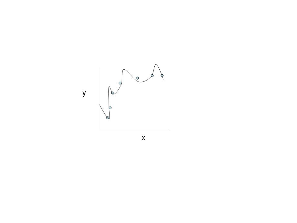
11. Team Batting Partnership plots

Graphical plot of batting partnerships for the countries

# Plot of batting partnerships of India (Virat Kohli and M S Dhoni have the best partnerships)
teamBatsmenPartnershipAllOppnAllMatchesPlot(ind_matches,"India",main="India")

batsmenPartnership1-1

# Plot of batting partnerships of Pakistan
teamBatsmenPartnershipAllOppnAllMatchesPlot(pak_matches,"Pakistan",main="Pakistan")

batsmenPartnership1-2

# Plot of batting partnerships of Australia
teamBatsmenPartnershipAllOppnAllMatchesPlot(aus_matches,"Australia",main="Australia")

batsmenPartnership1-3

12. Top opposition batting partnerships.

This gives the best performance of the team against a specified country Indian partnetships against Australia

New Zealand Partnetship against South Africa

# Top India partnerships against West Indies
teamBatsmenPartnershipAllOppnAllMatchesPlot(ind_matches,"India",main="West Indies")

batsmenPartnership2-1

# Top Sri Lanka parnerships ahgains India
teamBatsmenPartnershipAllOppnAllMatchesPlot(sl_matches,"Sri Lanka",main="India")

batsmenPartnership2-2

# Top New Zealand partnerships against South Africa
teamBatsmenPartnershipAllOppnAllMatchesPlot(nz_matches,"New Zealand",main="South Africa")

batsmenPartnership2-3

13. Batsmen vs Bowlers

The function below gives the top performance of batsmen against the opposition countries

# Top batsmen against bowlers when rank=0
m <-teamBatsmenVsBowlersAllOppnAllMatchesRept(ind_matches,"India",rank=0)
m
## Source: local data frame [68 x 2]
## 
##         batsman runsScored
##          (fctr)      (dbl)
## 1       V Kohli       7039
## 2      MS Dhoni       6885
## 3      SK Raina       4964
## 4     G Gambhir       4503
## 5     RG Sharma       4385
## 6  SR Tendulkar       4196
## 7  Yuvraj Singh       3976
## 8      V Sehwag       3681
## 9      S Dhawan       2694
## 10    AM Rahane       2009
## ..          ...        ...
# Performance of India batsman with rank=1 against international bowlers and runs scored against bowlers. This is Virat Kohli for India
m <-teamBatsmenVsBowlersAllOppnAllMatchesRept(ind_matches,"India",rank=1,dispRows=30)
m
## Source: local data frame [30 x 3]
## Groups: batsman [1]
## 
##    batsman          bowler  runs
##     (fctr)          (fctr) (dbl)
## 1  V Kohli     NLTC Perera   242
## 2  V Kohli KMDN Kulasekara   196
## 3  V Kohli      SL Malinga   175
## 4  V Kohli      AD Mathews   155
## 5  V Kohli      BAW Mendis   132
## 6  V Kohli       R Rampaul   127
## 7  V Kohli     JW Dernbach   121
## 8  V Kohli     JP Faulkner   118
## 9  V Kohli       DJG Sammy   116
## 10 V Kohli    HMRKB Herath   113
## ..     ...             ...   ...
# Performance of India batsman with rank=2 against international bowlers and runs scored against these bowlers. This is M S Dhoni for India
m <-teamBatsmenVsBowlersAllOppnAllMatchesRept(ind_matches,"India",rank=2,dispRows=50)
m
## Source: local data frame [50 x 3]
## Groups: batsman [1]
## 
##     batsman         bowler  runs
##      (fctr)         (fctr) (dbl)
## 1  MS Dhoni M Muralitharan   195
## 2  MS Dhoni  ST Jayasuriya   183
## 3  MS Dhoni     SL Malinga   144
## 4  MS Dhoni      SR Watson   135
## 5  MS Dhoni        ST Finn   130
## 6  MS Dhoni     MG Johnson   128
## 7  MS Dhoni    JP Faulkner   125
## 8  MS Dhoni  Shahid Afridi   120
## 9  MS Dhoni     TT Bresnan   111
## 10 MS Dhoni     AD Mathews   111
## ..      ...            ...   ...
# Performance of England batsman with rank=1 against international bowlers and runs scored against these bowlers. This returns a data frame of the the theTeam's batsmen against the bowlers for which the 'matches' dataframe is used. This Is IR Bell,
m <-teamBatsmenVsBowlersAllOppnAllMatchesRept(matches=ind_matches,theTeam="England",rank=1,dispRows=25)
m
## Source: local data frame [25 x 3]
## Groups: batsman [1]
## 
##    batsman       bowler  runs
##     (fctr)       (fctr) (dbl)
## 1  IR Bell       Z Khan   127
## 2  IR Bell    PP Chawla   111
## 3  IR Bell    RA Jadeja    94
## 4  IR Bell      B Kumar    78
## 5  IR Bell     MM Patel    77
## 6  IR Bell     R Ashwin    71
## 7  IR Bell   AB Agarkar    66
## 8  IR Bell     I Sharma    57
## 9  IR Bell     RP Singh    51
## 10 IR Bell Yuvraj Singh    51
## ..     ...          ...   ...
# All the best Australian batsmen against India in all of Indian matches
m <-teamBatsmenVsBowlersAllOppnAllMatchesRept(ind_matches,"Australia",rank=0)
m
## Source: local data frame [47 x 2]
## 
##       batsman runsScored
##        (fctr)      (dbl)
## 1  RT Ponting        876
## 2  MEK Hussey        753
## 3   GJ Bailey        614
## 4   SR Watson        609
## 5   MJ Clarke        607
## 6   ML Hayden        573
## 7   A Symonds        536
## 8    AJ Finch        525
## 9   SPD Smith        467
## 10  DA Warner        391
## ..        ...        ...

14. Batsmen vs Bowlers (continued)

# The best India batsman(rank=0) against England and his performance against England bowlers
m <-teamBatsmenVsBowlersAllOppnAllMatchesRept(eng_matches,"India",rank=1,dispRows=30)
m
## Source: local data frame [28 x 3]
## Groups: batsman [1]
## 
##     batsman      bowler  runs
##      (fctr)      (fctr) (dbl)
## 1  MS Dhoni     ST Finn   130
## 2  MS Dhoni  TT Bresnan   111
## 3  MS Dhoni    GP Swann   101
## 4  MS Dhoni JW Dernbach    95
## 5  MS Dhoni   SCJ Broad    92
## 6  MS Dhoni JM Anderson    89
## 7  MS Dhoni    SR Patel    83
## 8  MS Dhoni JC Tredwell    40
## 9  MS Dhoni   CR Woakes    38
## 10 MS Dhoni  MS Panesar    37
## ..      ...         ...   ...
# All the top Sri Lanka batsmen (rank=0) against Australia and performances against Australian bowlers
m <-teamBatsmenVsBowlersAllOppnAllMatchesRept(aus_matches,"Sri Lanka",rank=0)
m
## Source: local data frame [31 x 2]
## 
##             batsman runsScored
##              (fctr)      (dbl)
## 1     KC Sangakkara        888
## 2  DPMD Jayawardene        846
## 3        TM Dilshan        799
## 4       WU Tharanga        464
## 5      LD Chandimal        413
## 6        AD Mathews        404
## 7   HDRL Thirimanne        290
## 8   KMDN Kulasekara        232
## 9     ST Jayasuriya        117
## 10       SL Malinga         91
## ..              ...        ...
#All the top England batsmen (rank=0) and their performances against South African bowlers
m <-teamBatsmenVsBowlersAllOppnAllMatchesRept(sa_matches,"England",rank=0)
m
## Source: local data frame [39 x 2]
## 
##           batsman runsScored
##            (fctr)      (dbl)
## 1       IJL Trott        424
## 2         JE Root        372
## 3         IR Bell        362
## 4      EJG Morgan        335
## 5  PD Collingwood        319
## 6        AD Hales        271
## 7    KP Pietersen        192
## 8      A Flintoff        192
## 9         OA Shah        177
## 10     JC Buttler        154
## ..            ...        ...

15. Batsmen vs Bowlers Plot

The following functions plot the performances of the batsman based on the rank chosen against opposition bowlers. Note: The rank has to be >0

#The following plot displays the performance of the top India batsman (rank=1) against all opposition bowlers. This is Virat Kohli for India

d <- teamBatsmenVsBowlersAllOppnAllMatchesRept(ind_matches,"India",rank=1,dispRows=50)
d
## Source: local data frame [50 x 3]
## Groups: batsman [1]
## 
##    batsman          bowler  runs
##     (fctr)          (fctr) (dbl)
## 1  V Kohli     NLTC Perera   242
## 2  V Kohli KMDN Kulasekara   196
## 3  V Kohli      SL Malinga   175
## 4  V Kohli      AD Mathews   155
## 5  V Kohli      BAW Mendis   132
## 6  V Kohli       R Rampaul   127
## 7  V Kohli     JW Dernbach   121
## 8  V Kohli     JP Faulkner   118
## 9  V Kohli       DJG Sammy   116
## 10 V Kohli    HMRKB Herath   113
## ..     ...             ...   ...
teamBatsmenVsBowlersAllOppnAllMatchesPlot(d)

batsmenVsBowler1-1

e <- teamBatsmenVsBowlersAllOppnAllMatchesPlot(d,plot=FALSE)
e
## Source: local data frame [50 x 3]
## Groups: batsman [1]
## 
##    batsman          bowler  runs
##     (fctr)          (fctr) (dbl)
## 1  V Kohli     NLTC Perera   242
## 2  V Kohli KMDN Kulasekara   196
## 3  V Kohli      SL Malinga   175
## 4  V Kohli      AD Mathews   155
## 5  V Kohli      BAW Mendis   132
## 6  V Kohli       R Rampaul   127
## 7  V Kohli     JW Dernbach   121
## 8  V Kohli     JP Faulkner   118
## 9  V Kohli       DJG Sammy   116
## 10 V Kohli    HMRKB Herath   113
## ..     ...             ...   ...
# The following plot displays the performance of the batsman (rank=2) against all opposition bowlers. This is M S Dhoni for India
d <- teamBatsmenVsBowlersAllOppnAllMatchesRept(ind_matches,"India",rank=2,dispRows=50)
teamBatsmenVsBowlersAllOppnAllMatchesPlot(d)

batsmenVsBowler1-2

# Best batsman of South Africa against Indian  bowlers
d <- teamBatsmenVsBowlersAllOppnAllMatchesRept(ind_matches,"South Africa",rank=1,dispRows=30)
d
## Source: local data frame [30 x 3]
## Groups: batsman [1]
## 
##           batsman          bowler  runs
##            (fctr)          (fctr) (dbl)
## 1  AB de Villiers Harbhajan Singh   133
## 2  AB de Villiers         B Kumar    93
## 3  AB de Villiers       RA Jadeja    90
## 4  AB de Villiers        A Mishra    77
## 5  AB de Villiers       MM Sharma    68
## 6  AB de Villiers          Z Khan    65
## 7  AB de Villiers     S Sreesanth    61
## 8  AB de Villiers         A Nehra    58
## 9  AB de Villiers        R Ashwin    55
## 10 AB de Villiers       IK Pathan    45
## ..            ...             ...   ...
teamBatsmenVsBowlersAllOppnAllMatchesPlot(d)

batsmenVsBowler1-3

# Best batsman of England (rank=1) against Indian bowlers (matches=ind_matches)
d <-teamBatsmenVsBowlersAllOppnAllMatchesRept(matches=ind_matches,"England",rank=1,dispRows=50)
d
## Source: local data frame [28 x 3]
## Groups: batsman [1]
## 
##    batsman       bowler  runs
##     (fctr)       (fctr) (dbl)
## 1  IR Bell       Z Khan   127
## 2  IR Bell    PP Chawla   111
## 3  IR Bell    RA Jadeja    94
## 4  IR Bell      B Kumar    78
## 5  IR Bell     MM Patel    77
## 6  IR Bell     R Ashwin    71
## 7  IR Bell   AB Agarkar    66
## 8  IR Bell     I Sharma    57
## 9  IR Bell     RP Singh    51
## 10 IR Bell Yuvraj Singh    51
## ..     ...          ...   ...
teamBatsmenVsBowlersAllOppnAllMatchesPlot(d)

batsmenVsBowler1-4

15. Batsmen vs Bowlers Plot (continued)

# Top batsman of South Africa and performance against opposition bowlers of all countries
d <- teamBatsmenVsBowlersAllOppnAllMatchesRept(sa_matches,"South Africa",rank=1,dispRows=50)
d
## Source: local data frame [50 x 3]
## Groups: batsman [1]
## 
##           batsman          bowler  runs
##            (fctr)          (fctr) (dbl)
## 1  AB de Villiers   Shahid Afridi   227
## 2  AB de Villiers     Saeed Ajmal   174
## 3  AB de Villiers Mohammad Hafeez   151
## 4  AB de Villiers       JO Holder   138
## 5  AB de Villiers Harbhajan Singh   133
## 6  AB de Villiers      Wahab Riaz   130
## 7  AB de Villiers      MG Johnson   129
## 8  AB de Villiers        P Utseya   128
## 9  AB de Villiers       DJG Sammy   110
## 10 AB de Villiers        DJ Bravo   107
## ..            ...             ...   ...
teamBatsmenVsBowlersAllOppnAllMatchesPlot(d)

batsmenVsBowler2-1

# Do not display plot but return dataframe
e <- teamBatsmenVsBowlersAllOppnAllMatchesPlot(d,plot=FALSE)
e
## Source: local data frame [50 x 3]
## Groups: batsman [1]
## 
##           batsman          bowler  runs
##            (fctr)          (fctr) (dbl)
## 1  AB de Villiers   Shahid Afridi   227
## 2  AB de Villiers     Saeed Ajmal   174
## 3  AB de Villiers Mohammad Hafeez   151
## 4  AB de Villiers       JO Holder   138
## 5  AB de Villiers Harbhajan Singh   133
## 6  AB de Villiers      Wahab Riaz   130
## 7  AB de Villiers      MG Johnson   129
## 8  AB de Villiers        P Utseya   128
## 9  AB de Villiers       DJG Sammy   110
## 10 AB de Villiers        DJ Bravo   107
## ..            ...             ...   ...
# Top batsman of Sri Lanka against bowlers of all countries
d <- teamBatsmenVsBowlersAllOppnAllMatchesRept(sl_matches,"Sri Lanka",rank=1,dispRows=50)
teamBatsmenVsBowlersAllOppnAllMatchesPlot(d)

batsmenVsBowler2-2

# Best West Indian against English bowlrs
d <- teamBatsmenVsBowlersAllOppnAllMatchesRept(eng_matches,"West Indies",rank=1,dispRows=50)
teamBatsmenVsBowlersAllOppnAllMatchesPlot(d)

batsmenVsBowler2-3

16 Team bowling scorecard against all opposition

The functions lists the top bowlers of each country in ODI matches. This function returns a dataframe when ‘matches’ is the matches of the country and ‘theTeam’ is the same country as in the functions below

teamBowlingScorecardAllOppnAllMatchesMain(matches=ind_matches,theTeam="India")
## Source: local data frame [57 x 5]
## 
##             bowler overs maidens  runs wickets
##             (fctr) (int)   (int) (dbl)   (dbl)
## 1        RA Jadeja    43       0  4749     153
## 2         R Ashwin    49       0  4225     146
## 3           Z Khan    47       0  3692     141
## 4  Harbhajan Singh    45       0  4040     123
## 5         I Sharma    51       0  3216     113
## 6         MM Patel    49       1  2400      92
## 7          P Kumar    50       2  2752      84
## 8         UT Yadav    51       0  2442      80
## 9   Mohammed Shami    43       0  1806      80
## 10    Yuvraj Singh    38       0  2588      77
## ..             ...   ...     ...   ...     ...
teamBowlingScorecardAllOppnAllMatchesMain(matches=aus_matches,theTeam="Australia")
## Source: local data frame [54 x 5]
## 
##          bowler overs maidens  runs wickets
##          (fctr) (int)   (int) (dbl)   (dbl)
## 1    MG Johnson    51       0  5635     245
## 2         B Lee    50       0  3400     147
## 3     SR Watson    45      NA    NA     136
## 4    NW Bracken    51       0  2763     114
## 5      CJ McKay    49      NA    NA     103
## 6      MA Starc    48       1  1769      97
## 7   JP Faulkner    44       0  2004      75
## 8      JR Hopes    43       0  2098      69
## 9       SW Tait    50       0  1461      66
## 10 DE Bollinger    51       0  1482      65
## ..          ...   ...     ...   ...     ...
teamBowlingScorecardAllOppnAllMatchesMain(eng_matches,"England")
## Source: local data frame [52 x 5]
## 
##            bowler overs maidens  runs wickets
##            (fctr) (int)   (int) (dbl)   (dbl)
## 1     JM Anderson    51       0  5688     202
## 2       SCJ Broad    51       0  5160     198
## 3      TT Bresnan    51       0  3730     117
## 4         ST Finn    49       0  2839     106
## 5        GP Swann    39       0  2760     106
## 6  PD Collingwood    40       1  2517      77
## 7      A Flintoff    45       0  1260      68
## 8     JC Tredwell    42       0  1614      62
## 9       CR Woakes    47       0  1859      57
## 10      RS Bopara    34       0  1508      42
## ..            ...   ...     ...   ...     ...
teamBowlingScorecardAllOppnAllMatchesMain(pak_matches,"Pakistan")
## Source: local data frame [55 x 5]
## 
##             bowler overs maidens  runs wickets
##             (fctr) (int)   (int) (dbl)   (dbl)
## 1    Shahid Afridi    45       0  6674     212
## 2      Saeed Ajmal    44       0  4089     184
## 3         Umar Gul    49       0  4127     151
## 4       Wahab Riaz    50       0  2954     111
## 5  Mohammad Hafeez    51       0  3502     109
## 6   Mohammad Irfan    49       0  2523      86
## 7    Sohail Tanvir    48       1  2534      75
## 8      Junaid Khan    48       1  2056      75
## 9   Iftikhar Anjum    49       2  1674      62
## 10    Shoaib Malik    41       1  2206      59
## ..             ...   ...     ...   ...     ...
teamBowlingScorecardAllOppnAllMatchesMain(sa_matches,"South Africa")
## Source: local data frame [41 x 5]
## 
##           bowler overs maidens  runs wickets
##           (fctr) (int)   (int) (dbl)   (dbl)
## 1       DW Steyn    51       0  4294     179
## 2       M Morkel    51       0  4012     172
## 3    LL Tsotsobe    42       0  2231     100
## 4    Imran Tahir    39       0  2124      93
## 5      R McLaren    41       1  1983      80
## 6      JH Kallis    44       0  2075      77
## 7     WD Parnell    44       0  1957      74
## 8        J Botha    44       0  2311      69
## 9    RJ Peterson    47       1  1872      68
## 10 CK Langeveldt    49       0  1829      65
## ..           ...   ...     ...   ...     ...
teamBowlingScorecardAllOppnAllMatchesMain(nz_matches,"New Zealand")
## Source: local data frame [51 x 5]
## 
##            bowler overs maidens  runs wickets
##            (fctr) (int)   (int) (dbl)   (dbl)
## 1        KD Mills    50       1  3918     160
## 2      DL Vettori    43       1  3767     147
## 3      TG Southee    51       0  3996     134
## 4  MJ McClenaghan    49       0  2252      85
## 5        JDP Oram    46       0  2064      78
## 6     NL McCullum    46       0  2840      67
## 7         SE Bond    37       1  1449      62
## 8        TA Boult    40       3  1324      58
## 9     CJ Anderson    41       0  1297      52
## 10       MJ Henry    41       0  1098      47
## ..            ...   ...     ...   ...     ...
teamBowlingScorecardAllOppnAllMatchesMain(sl_matches,"Sri Lanka")
## Source: local data frame [54 x 5]
## 
##             bowler overs maidens  runs wickets
##             (fctr) (int)   (int) (dbl)   (dbl)
## 1       SL Malinga    51       0  7214     281
## 2  KMDN Kulasekara    51       0  5481     179
## 3       BAW Mendis    47       0  2979     135
## 4      NLTC Perera    48       0  3624     129
## 5   M Muralitharan    45       0  2471     114
## 6       AD Mathews    51       0  3394     113
## 7       TM Dilshan    50       0  3049      73
## 8     CRD Fernando    51       1  2067      73
## 9     HMRKB Herath    41       0  2027      71
## 10     MF Maharoof    48       0  1860      70
## ..             ...   ...     ...   ...     ...
teamBowlingScorecardAllOppnAllMatchesMain(wi_matches,"West Indies")
## Source: local data frame [45 x 5]
## 
##        bowler overs maidens  runs wickets
##        (fctr) (int)   (int) (dbl)   (dbl)
## 1    DJ Bravo    51       0  4239     153
## 2   JE Taylor    50       0  2530     103
## 3   R Rampaul    46       1  2608     102
## 4   KAJ Roach    49       0  2500      98
## 5   SP Narine    47       0  1924      82
## 6   DJG Sammy    51       1  3584      79
## 7  AD Russell    48       0  1987      63
## 8    CH Gayle    38       0  1955      53
## 9   JO Holder    44       0  1542      50
## 10 MN Samuels    38       0  2209      48
## ..        ...   ...     ...   ...     ...

17 Team bowling scorecard against all opposition (continued)

The function lists the top bowlers of a country (‘matches’) against the opposition country

# Best Indian bowlers in matches against Australia
teamBowlingScorecardAllOppnAllMatches(ind_matches,'Australia')
## Source: local data frame [36 x 5]
## 
##             bowler overs maidens  runs wickets
##             (fctr) (int)   (int) (dbl)   (dbl)
## 1         I Sharma    44       1   739      26
## 2  Harbhajan Singh    40       0   926      25
## 3        IK Pathan    42       1   702      22
## 4         UT Yadav    37       2   606      18
## 5      S Sreesanth    34       0   454      18
## 6        RA Jadeja    39       0   867      16
## 7           Z Khan    33       1   500      15
## 8         R Ashwin    43       0   684      14
## 9          P Kumar    27       0   501      14
## 10   R Vinay Kumar    31       1   380      14
## ..             ...   ...     ...   ...     ...
# Best Australian bowlers in matches against India
teamBowlingScorecardAllOppnAllMatches(aus_matches,'India')
## Source: local data frame [39 x 5]
## 
##         bowler overs maidens  runs wickets
##         (fctr) (int)   (int) (dbl)   (dbl)
## 1   MG Johnson    47       0  1020      44
## 2        B Lee    41       3   671      28
## 3    SR Watson    36       1   532      18
## 4     CJ McKay    37       1   403      18
## 5      GB Hogg    33       0   427      17
## 6  JP Faulkner    26       0   598      16
## 7     JR Hopes    31       0   346      14
## 8   NW Bracken    35       1   429      13
## 9  JW Hastings    27       2   259      13
## 10    MA Starc    26       0   251      13
## ..         ...   ...     ...   ...     ...
# Best New Zealand bowlers in matches against England
teamBowlingScorecardAllOppnAllMatches(nz_matches,'England')
## Source: local data frame [33 x 5]
## 
##            bowler overs maidens  runs wickets
##            (fctr) (int)   (int) (dbl)   (dbl)
## 1      TG Southee    39       2   684      33
## 2      DL Vettori    27       1   561      28
## 3        KD Mills    27       0   742      24
## 4  MJ McClenaghan    25       1   515      20
## 5    JEC Franklin    23       0   418      12
## 6         SE Bond    16       0   205      12
## 7      GD Elliott    10       3   194      12
## 8       SB Styris     8       0   296       9
## 9     NL McCullum    24       0   425       7
## 10     MJ Santner    18       0   230       7
## ..            ...   ...     ...   ...     ...
# Best Sri Lankan bowlers in matches against West Indies
teamBowlingScorecardAllOppnAllMatches(sl_matches,"West Indies")
## Source: local data frame [24 x 5]
## 
##             bowler overs maidens  runs wickets
##             (fctr) (int)   (int) (dbl)   (dbl)
## 1       SL Malinga    28       1   280      14
## 2       BAW Mendis    15       0   267       9
## 3  KMDN Kulasekara    13       1   185       8
## 4       AD Mathews    14       0   191       7
## 5   M Muralitharan    20       1   157       6
## 6      MF Maharoof     9       2    14       6
## 7       WPUJC Vaas     7       2    82       5
## 8       RAS Lakmal     7       0    55       5
## 9     HMRKB Herath    10       1   124       4
## 10   ST Jayasuriya     1       0    38       4
## ..             ...   ...     ...   ...     ...

18. Team Bowlers versus Batsmen (against all oppositions)

The functions below give the peformance of bowlers versus batsman. They give the best bowlers and the total runs conceded and against whom were the runs conceded

# Best bowlers overall from India against all opposition (rank=0)
teamBowlersVsBatsmenAllOppnAllMatchesMain(ind_matches,theTeam="India",rank=0)
## Source: local data frame [10 x 2]
## 
##             bowler  runs
##             (fctr) (dbl)
## 1        RA Jadeja  4691
## 2         R Ashwin  4111
## 3  Harbhajan Singh  3858
## 4           Z Khan  3514
## 5         I Sharma  3100
## 6          P Kumar  2646
## 7     Yuvraj Singh  2542
## 8        IK Pathan  2359
## 9         UT Yadav  2343
## 10        MM Patel  2314
# Top ODI bowler of India and runs conceded against different opposition batsmen 
(rank=1)
## [1] 1
m <-teamBowlersVsBatsmenAllOppnAllMatchesMain(ind_matches,theTeam="India",rank=1)
m
## Source: local data frame [207 x 3]
## Groups: bowler [1]
## 
##       bowler          batsman runsConceded
##       (fctr)           (fctr)        (dbl)
## 1  RA Jadeja    KC Sangakkara          172
## 2  RA Jadeja DPMD Jayawardene          117
## 3  RA Jadeja       TM Dilshan          108
## 4  RA Jadeja     LD Chandimal          103
## 5  RA Jadeja        GJ Bailey           99
## 6  RA Jadeja      LRPL Taylor           95
## 7  RA Jadeja          IR Bell           94
## 8  RA Jadeja    KS Williamson           92
## 9  RA Jadeja   AB de Villiers           90
## 10 RA Jadeja        SR Watson           85
## ..       ...              ...          ...
# Top ODI bowler of India and runs conceded against different opposition batsmen (rank=2)
m <-teamBowlersVsBatsmenAllOppnAllMatchesMain(ind_matches,theTeam="India",rank=2)
m
## Source: local data frame [177 x 3]
## Groups: bowler [1]
## 
##      bowler          batsman runsConceded
##      (fctr)           (fctr)        (dbl)
## 1  R Ashwin        GJ Bailey          132
## 2  R Ashwin    KC Sangakkara          117
## 3  R Ashwin          AN Cook          115
## 4  R Ashwin    KS Williamson          114
## 5  R Ashwin         DM Bravo          111
## 6  R Ashwin       AD Mathews          100
## 7  R Ashwin     LD Chandimal           98
## 8  R Ashwin      LRPL Taylor           93
## 9  R Ashwin DPMD Jayawardene           93
## 10 R Ashwin     KP Pietersen           81
## ..      ...              ...          ...

18. Team Bowlers versus Batsmen (against all oppositions continued)

# Top bowlers versus batsmen of South Africa(rank=0)
teamBowlersVsBatsmenAllOppnAllMatchesMain(sa_matches,theTeam="South Africa",rank=0)
## Source: local data frame [10 x 2]
## 
##         bowler  runs
##         (fctr) (dbl)
## 1     DW Steyn  4116
## 2     M Morkel  3808
## 3      J Botha  2244
## 4  LL Tsotsobe  2147
## 5    JP Duminy  2111
## 6  Imran Tahir  2087
## 7    JH Kallis  2014
## 8   WD Parnell  1864
## 9    R McLaren  1863
## 10 RJ Peterson  1842
# Top bowlers versus batsmen of Pakistan(rank=0)
teamBowlersVsBatsmenAllOppnAllMatchesMain(pak_matches,theTeam="Pakistan",rank=0)
## Source: local data frame [10 x 2]
## 
##             bowler  runs
##             (fctr) (dbl)
## 1    Shahid Afridi  6444
## 2      Saeed Ajmal  3956
## 3         Umar Gul  3901
## 4  Mohammad Hafeez  3434
## 5       Wahab Riaz  2755
## 6   Mohammad Irfan  2399
## 7    Sohail Tanvir  2337
## 8     Shoaib Malik  2105
## 9      Junaid Khan  1974
## 10  Iftikhar Anjum  1626
# Top bowlers versus batsmen of Sri Lanka(rank=0)
teamBowlersVsBatsmenAllOppnAllMatchesMain(sl_matches,theTeam="Sri Lanka",rank=1)
## Source: local data frame [314 x 3]
## Groups: bowler [1]
## 
##        bowler         batsman runsConceded
##        (fctr)          (fctr)        (dbl)
## 1  SL Malinga Mohammad Hafeez          191
## 2  SL Malinga         V Kohli          175
## 3  SL Malinga       G Gambhir          170
## 4  SL Malinga        MS Dhoni          144
## 5  SL Malinga      Umar Akmal          142
## 6  SL Malinga        V Sehwag          140
## 7  SL Malinga         IR Bell          134
## 8  SL Malinga    SR Tendulkar          133
## 9  SL Malinga   Ahmed Shehzad          121
## 10 SL Malinga         AN Cook          120
## ..        ...             ...          ...
m <-teamBowlersVsBatsmenAllOppnAllMatchesMain(ind_matches,theTeam="India",rank=2)
m
## Source: local data frame [177 x 3]
## Groups: bowler [1]
## 
##      bowler          batsman runsConceded
##      (fctr)           (fctr)        (dbl)
## 1  R Ashwin        GJ Bailey          132
## 2  R Ashwin    KC Sangakkara          117
## 3  R Ashwin          AN Cook          115
## 4  R Ashwin    KS Williamson          114
## 5  R Ashwin         DM Bravo          111
## 6  R Ashwin       AD Mathews          100
## 7  R Ashwin     LD Chandimal           98
## 8  R Ashwin      LRPL Taylor           93
## 9  R Ashwin DPMD Jayawardene           93
## 10 R Ashwin     KP Pietersen           81
## ..      ...              ...          ...

19. Team bowlers versus batsmen report (all oppositions)

#Top bowlers of other countries against India
teamBowlersVsBatsmenAllOppnAllMatchesRept(matches=ind_matches,theTeam="India",rank=0)
## Source: local data frame [10 x 2]
## 
##             bowler  runs
##             (fctr) (dbl)
## 1  KMDN Kulasekara  1448
## 2       SL Malinga  1319
## 3      NLTC Perera   959
## 4      JM Anderson   954
## 5       MG Johnson   939
## 6        SCJ Broad   877
## 7       BAW Mendis   783
## 8       AD Mathews   776
## 9          ST Finn   751
## 10      TT Bresnan   741
# Best performer against India is KMDN Kulasekar of Sri Lanka in ODIs
a <- teamBowlersVsBatsmenAllOppnAllMatchesRept(ind_matches,theTeam="India",rank=1)
a
## Source: local data frame [31 x 3]
## Groups: bowler [1]
## 
##             bowler      batsman runsConceded
##             (fctr)       (fctr)        (dbl)
## 1  KMDN Kulasekara     V Sehwag          199
## 2  KMDN Kulasekara      V Kohli          196
## 3  KMDN Kulasekara    G Gambhir          157
## 4  KMDN Kulasekara SR Tendulkar          127
## 5  KMDN Kulasekara Yuvraj Singh          118
## 6  KMDN Kulasekara    RG Sharma          114
## 7  KMDN Kulasekara     SK Raina          104
## 8  KMDN Kulasekara     MS Dhoni           80
## 9  KMDN Kulasekara   KD Karthik           56
## 10 KMDN Kulasekara   SC Ganguly           51
## ..             ...          ...          ...

20. Team bowlers versus batsmen report (all oppositions continued)

#Top Indian bowlers against Sri Lanka 
teamBowlersVsBatsmenAllOppnAllMatchesRept(matches=ind_matches,theTeam="Sri Lanka",rank=0)
## Source: local data frame [10 x 2]
## 
##             bowler  runs
##             (fctr) (dbl)
## 1           Z Khan  1141
## 2        RA Jadeja   882
## 3         I Sharma   855
## 4  Harbhajan Singh   805
## 5          P Kumar   758
## 6         R Ashwin   740
## 7        IK Pathan   678
## 8          A Nehra   584
## 9         UT Yadav   544
## 10        MM Patel   488
#Top Indian bowlers against England
teamBowlersVsBatsmenAllOppnAllMatchesRept(ind_matches,"England",rank=0)
## Source: local data frame [10 x 2]
## 
##          bowler  runs
##          (fctr) (dbl)
## 1      R Ashwin   777
## 2     RA Jadeja   735
## 3        Z Khan   507
## 4      MM Patel   463
## 5      RP Singh   410
## 6      I Sharma   396
## 7     PP Chawla   375
## 8  Yuvraj Singh   370
## 9       B Kumar   353
## 10   AB Agarkar   336

21. Team bowlers versus batsmen report (all oppositions coninued-1)

#Top ODI opposition bowlers against New Zealand
teamBowlersVsBatsmenAllOppnAllMatchesRept(nz_matches,theTeam="New Zealand",rank=0)
## Source: local data frame [10 x 2]
## 
##             bowler  runs
##             (fctr) (dbl)
## 1      JM Anderson   889
## 2       MG Johnson   828
## 3    Shahid Afridi   751
## 4  KMDN Kulasekara   728
## 5        SCJ Broad   638
## 6       NW Bracken   626
## 7       SL Malinga   601
## 8         DW Steyn   556
## 9          ST Finn   482
## 10       SR Watson   468
# Top ODI opposition bowlers against Australia
teamBowlersVsBatsmenAllOppnAllMatchesRept(aus_matches,"Australia",rank=0)
## Source: local data frame [10 x 2]
## 
##             bowler  runs
##             (fctr) (dbl)
## 1      JM Anderson  1211
## 2       TT Bresnan  1087
## 3       SL Malinga  1078
## 4        SCJ Broad   948
## 5  Harbhajan Singh   890
## 6       DL Vettori   883
## 7  KMDN Kulasekara   875
## 8         DW Steyn   872
## 9        RA Jadeja   853
## 10        DJ Bravo   830
# Top ODI bowlers against Sri Lanka
teamBowlersVsBatsmenAllOppnAllMatchesRept(sl_matches,"Sri Lanka",rank=0)
## Source: local data frame [10 x 2]
## 
##             bowler  runs
##             (fctr) (dbl)
## 1    Shahid Afridi  1177
## 2           Z Khan  1141
## 3        RA Jadeja   882
## 4         I Sharma   855
## 5      Saeed Ajmal   814
## 6  Harbhajan Singh   805
## 7  Mohammad Hafeez   774
## 8          P Kumar   758
## 9         R Ashwin   740
## 10        Umar Gul   718

22. Team bowlers versus batsmen report (all oppositions) plot

This function can only be used for rank>0 (rank=1,2,3..)

# Top ODI bowler against India (KMDN Kulasekara)
df <- teamBowlersVsBatsmenAllOppnAllMatchesRept(ind_matches,theTeam="India",rank=1)
teamBowlersVsBatsmenAllOppnAllMatchesPlot(df,"India","India")

bowlerVsbatsmen1-1

# Top ODI Indian bowler versus England (R Ashwin)
df <- teamBowlersVsBatsmenAllOppnAllMatchesRept(ind_matches,theTeam="England",rank=1)
teamBowlersVsBatsmenAllOppnAllMatchesPlot(df,"India","England")

bowlerVsbatsmen1-2

#Top ODI Indian bowler against West Indies (RA Jadeja)
df <- teamBowlersVsBatsmenAllOppnAllMatchesRept(ind_matches,theTeam="West Indies",rank=1)
teamBowlersVsBatsmenAllOppnAllMatchesPlot(df,"India","West Indies")

bowlerVsbatsmen1-3

23. Team bowlers versus batsmen plot (all oppositions)

#Top bowler against South Africa (Shahid Afridi)
df <- teamBowlersVsBatsmenAllOppnAllMatchesRept(sa_matches,theTeam="South Africa",rank=1)
teamBowlersVsBatsmenAllOppnAllMatchesPlot(df,"South Africa","South Africa")

bowlerVsbatsmen2-1

# Top  bowler versus Pakistan (SL Malinga)
df <- teamBowlersVsBatsmenAllOppnAllMatchesRept(pak_matches,theTeam="Pakistan",rank=1)
teamBowlersVsBatsmenAllOppnAllMatchesPlot(df,"Pakistan","Pakistan")

bowlerVsbatsmen2-2

24. Team Bowler Wicket Kind

# Top opposition bowlers against India and the kind of wickets
teamBowlingWicketKindAllOppnAllMatches(ind_matches,t1="India",t2="All")

bowlingWicketkind1-1

# Get the data frame. Do not plot
m <-teamBowlingWicketKindAllOppnAllMatches(ind_matches,t1="India",t2="All",plot=FALSE)
m
## Source: local data frame [34 x 3]
## Groups: bowler [?]
## 
##         bowler        wicketKind     m
##         (fctr)             (chr) (int)
## 1   MG Johnson            bowled     8
## 2   MG Johnson            caught    27
## 3   MG Johnson caught and bowled     1
## 4   MG Johnson               lbw     6
## 5   MG Johnson           run out     2
## 6  JM Anderson            bowled     4
## 7  JM Anderson            caught    25
## 8  JM Anderson               lbw     1
## 9  JM Anderson           run out     3
## 10     ST Finn            bowled    10
## ..         ...               ...   ...
# Best Indian bowlers against South Africa
teamBowlingWicketKindAllOppnAllMatches(ind_matches,t1="India",t2="South Africa")

bowlingWicketkind1-2

# Best Indian bowlers against Pakistan
teamBowlingWicketKindAllOppnAllMatches(ind_matches,t1="India",t2="Pakistan")

bowlingWicketkind1-3

25. Team Bowler Wicket Kind (continued)

# Best ODI opposition bowlers against  England
teamBowlingWicketKindAllOppnAllMatches(eng_matches,t1="England",t2="All")

bowlingWicketkind2-1

# Best ODI opposition bowlers  Australia
teamBowlingWicketKindAllOppnAllMatches(aus_matches,t1="Australia",t2="All")

bowlingWicketkind2-2

# Best bowlera against  Sri Lanka
teamBowlingWicketKindAllOppnAllMatches(sl_matches,t1="Sri Lanka",t2="All")

bowlingWicketkind2-3

26. Team Bowler Wicket Runs

# Opposition bowlers against India and runs conceded
teamBowlingWicketRunsAllOppnAllMatches(ind_matches,t1="India",t2="All",plot=TRUE)

bowlingWicketRuns1-1

# Opposition bowlers against India and runs conceded returned as dataframe
m <-teamBowlingWicketRunsAllOppnAllMatches(ind_matches,t1="India",t2="All",plot=FALSE)
m
## Source: local data frame [10 x 3]
## 
##             bowler runsConceded wickets
##             (fctr)        (dbl)   (dbl)
## 1       MG Johnson         1020      44
## 2  KMDN Kulasekara         1492      40
## 3         DW Steyn          714      34
## 4       BAW Mendis          810      34
## 5      JM Anderson          991      33
## 6       SL Malinga         1402      33
## 7       AD Mathews          800      31
## 8          ST Finn          775      30
## 9      NLTC Perera          983      30
## 10       SCJ Broad          903      29
# Top Indian bowlers and runs conceded
teamBowlingWicketRunsAllOppnAllMatches(ind_matches,t1="India",t2="Australia",plot=TRUE)

bowlingWicketRuns1-2

27. Team Bowler Wicket Runs (continued)

#Top opposition bowlers against Pakistan
teamBowlingWicketRunsAllOppnAllMatches(pak_matches,t1="Pakistan",t2="All",plot=TRUE)

bowlingWicketRuns2-1

#Top opposition bowlers against West Indies
teamBowlingWicketRunsAllOppnAllMatches(wi_matches,t1="West Indies",t2="All",plot=TRUE)

bowlingWicketRuns2-2

#Top opposition bowlers against Sri Lanka
teamBowlingWicketRunsAllOppnAllMatches(sl_matches,t1="Sri Lanka",t2="All",plot=TRUE)

bowlingWicketRuns2-3

#Top opposition bowlers against New Zealand
teamBowlingWicketRunsAllOppnAllMatches(nz_matches,t1="New Zealand",t2="All",plot=TRUE)

bowlingWicketRuns2-4

Conclusion

This post included all functions for a team in all matches against all oppositions. As before the data frames are already available. You can load the data and begin to use them. If more insights from the dataframe are possible do go ahead. But please do attribute the source to Cricheet (http://cricsheet.org), my package yorkr and my blog. Do give the functions a spin for yourself.

I will be coming up with the last part to my introduction to cricket package yorkr soon.

Watch this space!

Important note: Do check out my other posts using yorkr at yorkr-posts

You may also like

  1. Introducing cricketr! : An R package to analyze performances of cricketers
  2. Cricket analytics with cricketr
  3. Literacy in India: A deepR dive
  4. Simulating an Edge shape in Android
  5. Re-working the Lucy Richardson algorithm in OpenCV
  6. Design principles of scalable distributed systems 7.TWS-4: Gossip protocol: Epidemics and rumors to the rescue

Simplifying ML: Impact of degree of polynomial degree on bias & variance and other insights

This post takes off from my earlier post Simplifying Machine Learning: Bias, variance, regularization and odd facts- Part 4. As discussed earlier a poor hypothesis function could either underfit or overfit the data.  If the number of features selected were small of the order of 1 or 2 features, then we could plot the data and try to determine how the hypothesis function fits the data. We could also see whether the function is capable of predicting output target values for new data.

 However if the number of features were large for e.g. of the order of 10’s of features then there needs to be method by which one can determine if the learned hypotheses is a ‘just right’ fit for all the data.

Checkout my book ‘Deep Learning from first principles Second Edition- In vectorized Python, R and Octave’.  My book is available on Amazon  as paperback ($18.99) and in kindle version($9.99/Rs449).

You may also like my companion book “Practical Machine Learning with R and Python:Second Edition- Machine Learning in stereo” available in Amazon in paperback($12.99) and Kindle($9.99/Rs449) versions.


The following technique can be used to determine the ‘goodness’ of a hypothesis or how well the hypothesis can fit the data and can also generalize to new examples not in the training set.

Several insights on how to evaluate a hypothesis is  given below

Consider a hypothesis function

hƟ (x) = Ɵ0 + Ɵ1x1 + Ɵ2x22 + Ɵ3x33  +  Ɵ4x44

a1

The above hypothesis does not generalize well enough for new examples in the data set.

Let us assume that there 100 training examples or data sets. Instead of using the entire set of 100 examples to learn the hypothesis function, the data set is divided into training set and test set in a 70%:30% ratio respectively

The hypothesis is learned from the training set. The learned hypothesis is then checked against the 30% test set data to determine whether the hypothesis is able to generalize on the test set also.

This is done by determining the error when the hypothesis is used against the test set.

For linear regression the error is computed by determining the average mean square error of the output value against the actual value as follows

The test set error is computed as follows

Jtest(Ɵ) = 1/2mtest Σ(hƟ (xtest – ytesti)2

For logistic regression the test set error is similarly determined as

Jtest(Ɵ) = = 1/mtest Σ -ytest * log(hƟ (xtest))  – (1-ytest) * (log(1 – hƟ (xtest))

The idea is that the test set error should as low as possible.

Model selection

A typical problem in determining the hypothesis is to choose the degree of the polynomial or to choose an appropriate model for the hypothesis

The method that can be followed is to choose 10 polynomial models

  1. hƟ (x) = Ɵ0 + Ɵ1x1
  2. hƟ (x) = Ɵ0 + Ɵ1x1 + Ɵ2x22
  3. hƟ (x) = Ɵ0 + Ɵ1x12 + Ɵ2x22 + Ɵ3x33

Here‘d’ is the degree of the polynomial. One method is to train all the 10 models. Run each of the model’s hypotheses against the test set and then choose the model with the smallest error cost.

While this appears to a good technique to choose the best fit hypothesis, in reality it is not so. The reason is that the hypothesis chosen is based on the best fit and the least error for the test data. However this does not generalize well for examples not in the training or test set.

So the correct method is to divide the data into 3 sets  as 60:20:20 where 60% is the training set, 20% is used as a test set to determine the best fit and the remaining 20% is the cross-validation set.

The steps carried out against the data is

  1. Train all 10 models against the training set (60%)
  2. Compute the cost value J against the cross-validation set (20%)
  3. Determine the lowest cost model
  4. Use this model against the test set and determine the generalization error.

Degree of the polynomial versus bias and variance

How does the degree of the polynomial affect the bias and variance of a hypothesis?

Clearly for a given training set when the degree is low the hypothesis will underfit the data and there will be a high bias error. However when the degree of the polynomial is high then the fit will get better and better on the training set (Note: This does not imply a good generalization)

We run all the models with different polynomial degrees on the cross validation set. What we will observe is that when the degree of the polynomial is low then the error will be high. This error will decrease as the degree of the polynomial increases as we will tend to get a better fit. However the error will again increase as higher degree polynomials that overfit the training set will be a poor fit for the cross validation set.

This is shown below

a2

Effect of regularization on bias & variance

Here is the technique to choose the optimum value for the regularization parameter λ

When λ is small then Ɵi values are large and we tend to overfit the data set. Hence the training error will be low but the cross validation error will be high. However when λ is large then the values of Ɵi become negligible almost leading to a polynomial degree of 1. These will underfit the data and result in a high training error and a cross validation error. Hence the chosen value of λ should be such that the cross validation error is the lowest

a3

Plotting learning curves

This is another technique to identify if the learned hypothesis has a high bias or a high variance based on the number of training examples

A high bias indicates an underfit. When the number of samples in training set if low then the training error and cross validation error will be low as it will be easy to create a hypothesis if there are few training examples. As the number of samples increase the error will increase for the training set and will slightly decrease for the cross validation set. However for a high bias, or underfit, after a certain point increasing the number of samples will not change the error. This is the case of a high bias

a4

In the case of high variance where a high degree polynomial is used for the hypothesis the training error will be low for smaller number of training examples. As the number of training examples increase the error will increase slowly. The cross validation error will be high for lesser number of training samples but will slowly decrease as the number of samples grow as the hypothesis will learn better. Hence for the case of high variance increasing the number of samples in the training set size will decrease the gap between the cross validation and the training error as shown below

a5

Note: This post, line previous posts on Machine Learning,  is based on the Coursera course on Machine Learning by Professor Andrew Ng

Also see
1. My book ‘Practical Machine Learning in R and Python: Third edition’ on Amazon
2.My book ‘Deep Learning from first principles:Second Edition’ now on Amazon
3.The Clash of the Titans in Test and ODI cricket
4. Introducing QCSimulator: A 5-qubit quantum computing simulator in R
5.Latency, throughput implications for the Cloud
6. Simulating a Web Joint in Android
5. Pitching yorkpy … short of good length to IPL – Part 1

Simplifying Machine Learning: Bias, Variance, regularization and odd facts – Part 4

In both linear and logistic regression the choice of the degree of the polynomial for the hypothesis function is extremely critical. A low degree for the polynomial can result in an underfit, while a very high degree can overfit the data as shown below

41

The figure on the left the data is underfit as we try to fit the data with a first order polynomial which is a straight line. This is a case of strong ‘bias’

The rightmost figure a much higher polynomial is used. All the data points are covered by the polynomial curve however it is not effective in predicting other values. This is a case of overfitting or a high variance.

The middle figure is just right as it intuitively fits the data points the best possible way.

A similar problem exists with logistic regression as shown below

42

There are 2 ways to handle overfitting

a)      Reducing the number of features selected

b)      Using regularization

In regularization the magnitude of the parameters Ɵ is decreased to reduce the effect of overfitting

Hence if we choose a hypothesis function

hƟ (x) = Ɵ0 + Ɵ1x12 + Ɵ2x22 + Ɵ3x33 +  Ɵ4x44


The cost function for this without regularization as mentioned in earlier posts

J(Ɵ) = 1/2m Σ(hƟ (xi  – yi)2

Where the key is minimize the above function for the least error

The cost function with regularization becomes

J(Ɵ) = 1/2m Σ(hƟ (xi  – yi)2 + λ Σ Ɵj2


As can be seen the regularization now adds a factor Ɵj2  as a part of the cost function which needs to be minimized.

Hence with the regularization factor the problem of underfitting/overfitting can be solved

43

However the trick is determine the value of λ. If λ is too big then it would result in underfitting or resulting in a high bias.

Similarly the regularized equation for logistic regression is as shown below

J(Ɵ) = |1/m Σ  -y * log(hƟ (x))  – (1-y) * (log(1 – hƟ (x))  | + λ/2m Σ Ɵj2

Some tips suggested by Prof Andrew Ng while determining the parameters and features for regression

a)      Get as many training examples. It is worth spending more effort in getting as much examples

b)      Add additional features

c)      Observe changes to the learning algorithm with different values of λ

This post is continued in my next post – Simplifying ML: Impact of degree of polynomial on bias, variance and other insights

Note: This post, in line with my previous posts on Machine Learning,  is based on the Coursera course on Machine Learning by Professor Andrew Ng


Find me on Google+

Simplifying ML: Neural networks- Part 3

Neural networks try to overcome the shortcomings of logistic regression in which  we have to choose a non-linear hypothesis. Logistic regression requires that we choose an appropriate combination of polynomial terms and the order of the equation. The problem with this is sometimes we either tend to overfit or underfit. Neural networks allow the ability to learns new model parameters from the basis raw parameters.

The neural network is modeled on the neural networking ability of the human brain. The brain is made of trillions of neurons. Each neuron is a processing unit which has several inputs in the dendrites and an output the axon. The neurons communicate thro a combination of electro chemical signal at the synapses or the spaces between the neuron.

neuron

A neural network mimics the working of the neuron.

So in a neural network the features of the problem serve as input. For e.g in the case of being able to determine if a mail is spam or not the features could be the words in the subject line, the from address, the contents etc. Based on a combination of these features we need to classify whether the mail is spam or not.

31

The above diagram shows a simple neural network with features x1, x2, x3 and a bias unit x0


With a hypothesis function hƟ(x) = 1/(1 + e-x)

The edges from the features xi  are the model parameters Ɵ. In other words the edges represent weights.

A typical neural network is a network of many logistic units organized in layers. The output of each layer forms the input to the next subsequent layer. This is shown below

32

As can be seen in a multi-layer neural network at the left we have the features x1,x2, .. xn.

This at the layer becomes the activation unit. The key advantage of neural networks over regular logistic regression that learns the models parameters is that learned model parameters are input to the next subsequent layers which learn the model parameters more finely. Hence this gives a better fit for the combination of parameters.

The activation parameters at the next layer are

a12 = g(Ɵ101x0+ Ɵ111x1+ Ɵ121x2 + Ɵ131x3) where g is the logistic function or the sigmoid function discussed in my previous post Simplifying ML: Logistic regression – Part 2

33

Here a12 is the activation parameter at layer 1

Ɵ10 is the model parameter at layer 1 and is the 0th parameter. Similarly Ɵ11 is the model parameter at layer 1 and is the 1st parameter and so on.

Similarly the other activation parameters can be written as

a22 = g(Ɵ201x0+ Ɵ211x1+ Ɵ221x2 + Ɵ231x3)

a32 = g(Ɵ301x0+ Ɵ311x1+ Ɵ321x2 + Ɵ331x3)

hƟ(x) = a13 = g(Ɵ102a0+ Ɵ112a1+ Ɵ122a2 + Ɵ132a3  – (A)


The crux of neural networks is that instead of creating a hypothesis based on the set of raw features, the neural network with multiple hidden layers can learn its own features. In the equation (A) we can see that the hypothesis is not a function of the input raw features x1,x2,… xbut on a new set of features or the activation units a1,a2, … an . In other words the network has ‘learned’ its own features.

As mentioned above the output of each layer is the logistic function or the sigmoid function

The beauty of neural networks based on logistic functions is that we can easily realize the equivalent of logic gates like AND, OR, NOT, NOR etc.

The hypothesis for the above network would be

34

hƟ(x) = g(-30 + 20 * x1 + 20 * x2)

So for x1= 0 and x2 = 0 we would have

hƟ(x) = g(-30 + 0 + 0) = g(-30)

Since g(-30) < g(0) < 0.5 = 0

37

Similarly a NOT gate can be constructed with a neural network as follows

35

38

Neural networks can also be used for multi class classification.

36

Hence there are multiple advantages to neural networks. Neural networks are amenable to a) creating complex logic models of combinations of AND, NOT, OR gates

b) The model parameters are learned from the raw parameters and can be more flexible.

It appears that the interest in neural networks surged in the 1980s and then waned, The neural networks were similar to the above and were based on forward propagation. However it appears that in recent time’s backward propagation has been used successfully in areas of research known as ‘deep learning’

This is based on the Coursera course on Machine Learning by Professor Andrew Ng. A highy enjoyable and classic course!!!


Find me on Google+

Simplifying ML: Logistic regression – Part 2

Logistic regression is another class of Machine Learning algorithms which comes under supervised learning. In this regression technique we need to classify data. Take a look at my earlier post Simplifying Machine Learning algorithms – Part 1 I had discussed linear regression. For e.g if we had data on tumor sizes versus the fact that the tumor was benign or malignant, the question is whether given a tumor size we can predict whether this tumor would be benign or cancerous. So we need to have the ability to classify this data.

This is shown below

4

It is obvious that a line with a certain slope could easily separate the two.

As another example we could have an algorithm that is able to automatically classify mail as either spam or not spam based on the subject line. So for e.g if the subject line had words like medicine, prize, lottery etc we could with a fair degree of probability classify this as spam.

However some classification problems could be far more complex.  We may need to classify another problem as shown below.

5

From the above it can be seen that hypothesis function is second order equation which is either a circle or an ellipse.

In the case of logistic regression the hypothesis function should be able to switch between 2 values 0 or 1 almost like a transistor either being in cutoff or in saturation state.

In the case of logistic regression 0 <= hƟ <= 1

The hypothesis function uses function of the following form

g(z) = 1/(1 + e‑z)

and hƟ (x) = g(ƟTX)

6

The function g(z) shown above has the characteristic required for logistic regression as it has the following shape

The function rapidly asymptotes at 1 when hƟ (x) >= 0.5 and  hƟ (x) asymptotes to 0 when hƟ (x) < 0.5

As in linear regression we can have hypothesis function be of an appropriate order. So for e.g. in the ellipse figure above one could choose a hypothesis function as follows

hƟ (x) = Ɵ0 + Ɵ1x12 + Ɵ2x22 + Ɵ3x1 +  Ɵ4x2


or


hƟ (x) = 1/(1 + e –(Ɵ0 + Ɵ1×12 + Ɵ2×22 + Ɵ3×1 +  Ɵ4×2))

We could choose the general form of a circle which is

f(x) = ax2 + by2 +2gx + 2hy + d

The cost function for logistic regression is given below

Cost(hƟ (x),y) = { -log(hƟ (x))             if y = 1

-log(1 – hƟ (x)))       if y = 0

In the case of regression there was a single cost function which could determine the error of the data against the predicted value.

The cost in the event of logistic regression is given as above as a set of 2 equations one for the case where the data is 1 and another for the case where the data is 0.

The reason for this is as follows. If we consider y =1 as a positive value, then when our hypothesis correctly predicts 1 then we have a ‘true positive’ however if we predict 0 when it should be 1 then we have a false negative. Similarly when the data is 0 and we predict a 1 then this is the case of a false positive and if we correctly predict 0 when it is 0 it is true negative.

Here is the reason as how the cost function

Cost(hƟ (x),y) = { -log(hƟ (x))             if y = 1

-log(1 – hƟ (x)))       if y = 0

Was arrived at. By definition the cost function gives the error between the predicted value and the data value.

The logic for determining the appropriate function is as follows

For y = 1

y=1 & hypothesis = 1 then cost = 0

y= 1 & hypothesis = 0 then cost = Infinity

Similarly for y = 0

y = 0 & hypotheses  = 0 then cost = 0

y = 0 & hypothesis = 1 then cost = Infinity

and the the functions above serve exactly this purpose as can be seen

7

Hence the cost can be written as

J(Ɵ) = Cost(hƟ (x),y) = -y * log(hƟ (x))  – (1-y) * (log(1 – hƟ (x))

This is the same as the equation above

The same gradient descent algorithm can now be used to minimize the cost function

So we can iterate througj

Ɵj =   Ɵj – α δ/δ Ɵj J(Ɵ0, Ɵ1,… Ɵn)

This works out to a function that is similar to linear regression

Ɵj = Ɵj – α 1/m { Σ hƟ (xi) – yi} xj i

This will enable the machine to fairly accurately determine the parameters Ɵj for the features x and provide the hypothesis function.

This is based on the Coursera course on Machine Learning by Professor Andrew Ng. Highly recommended!!!

Find me on Google+