It is carnival time again as IPL 2023 is underway!! The new GooglyPlusPlus now includes AI/ML models for computing ball-by-ball Win Probability of matches and each individual player’s Win Probability Contribution (WPC). GooglyPlusPlus uses 2 ML models
Deep Learning (Tensorflow) – accuracy : 0.8584
Logistic Regression (glmnet-tidymodels) : 0.728
Besides, as before, GooglyPlusPlus will also include the usual near real-time analytics with the Shiny app being automatically updated with the previous day’s match data.
Note: The Win Probability Computation can also be done on a live feed of streaming data. Since, I don’t have access to live feeds, the app will show how Win Probability changed during the course of completed matches. For more details on Win Probability and Win Probability Contribution see my posts
GooglyPlusPlus has been also updated with all the latest T20 league’s match data. It includes data from BBL 2022, NTB 2022, CPL 2022, PSL 2023, ICC T20 2022 and now IPL 2023.
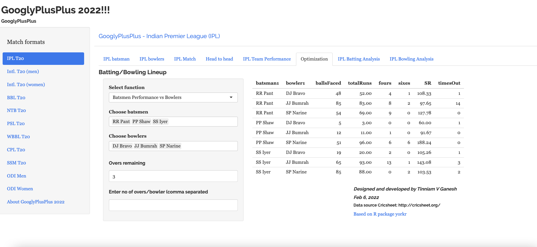
GooglyPlusPlus has the following functionality
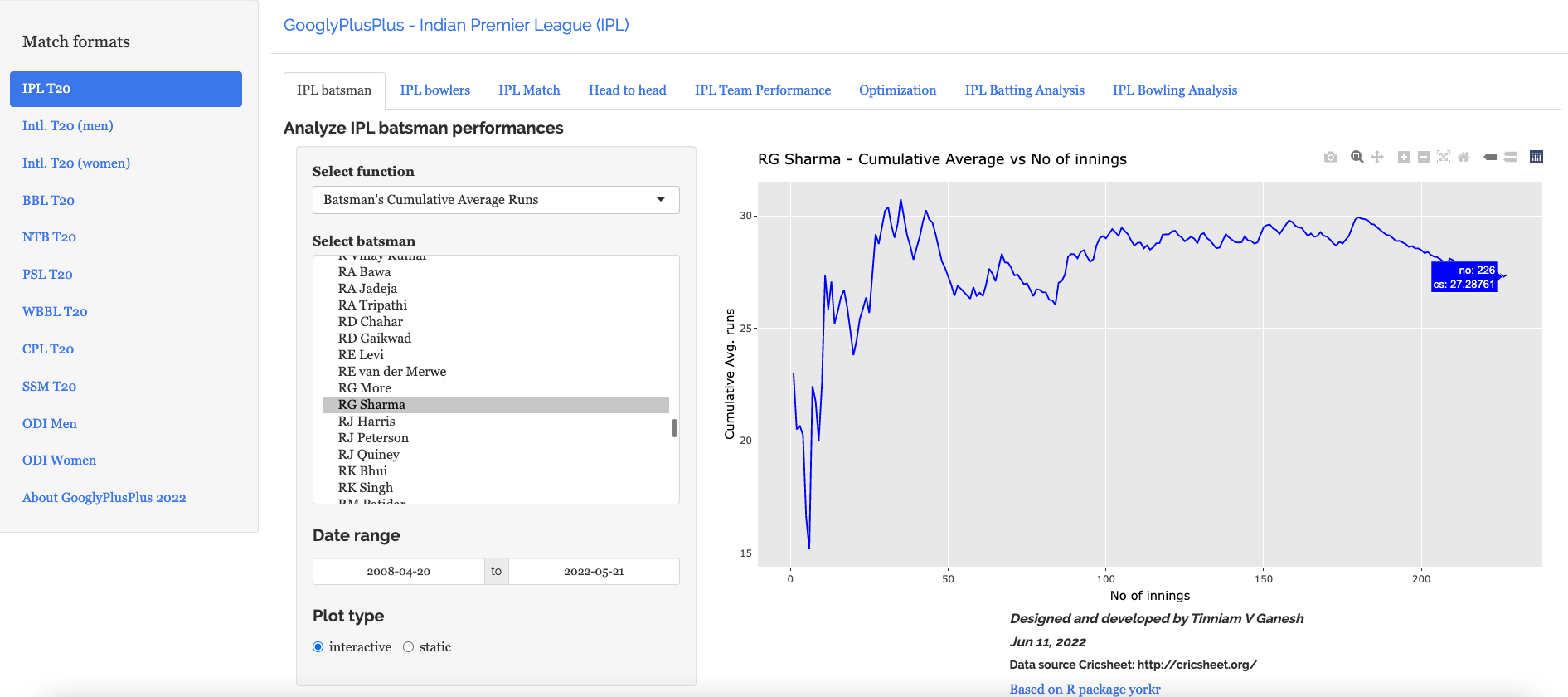
Batsman tab: For detailed analysis of batsmen
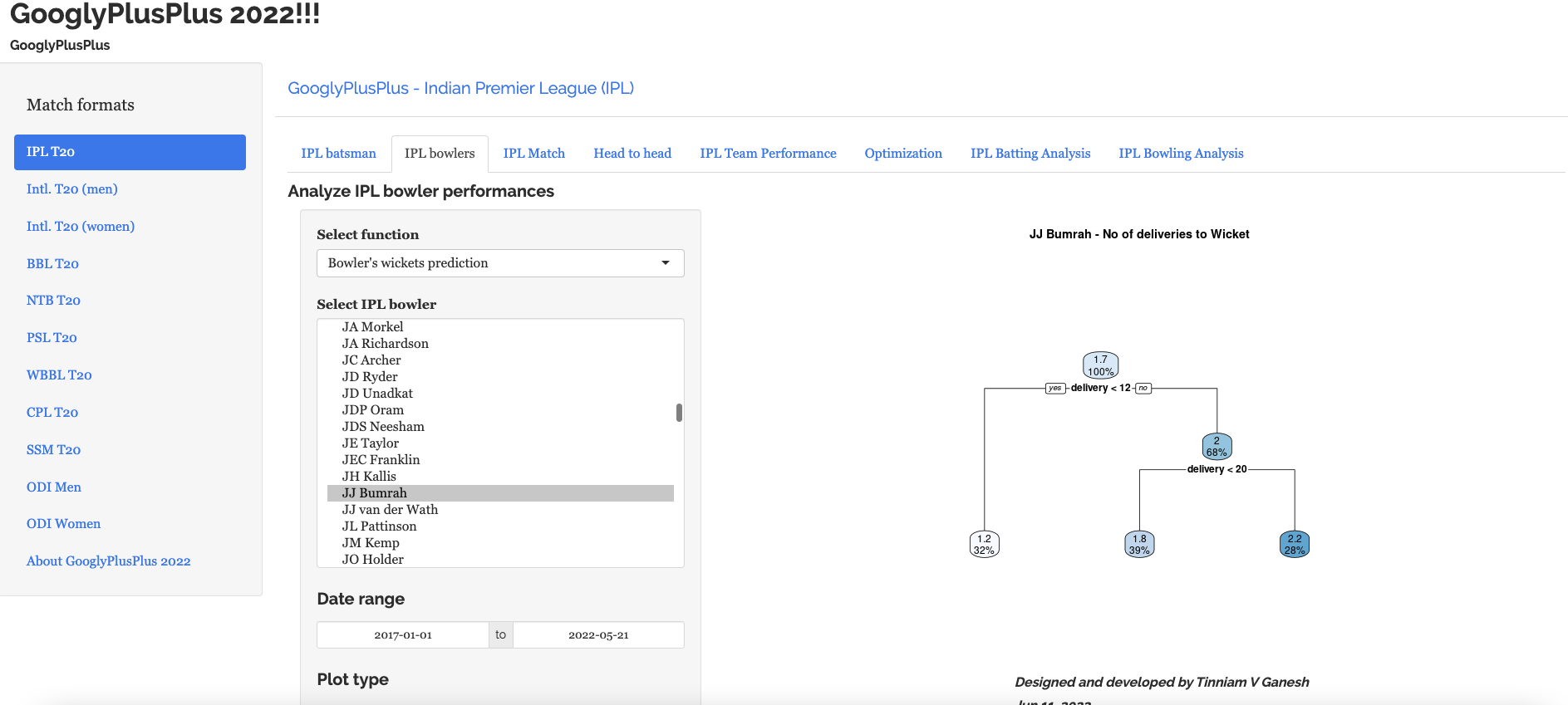
Bowler tab: For detailed analysis of bowlers
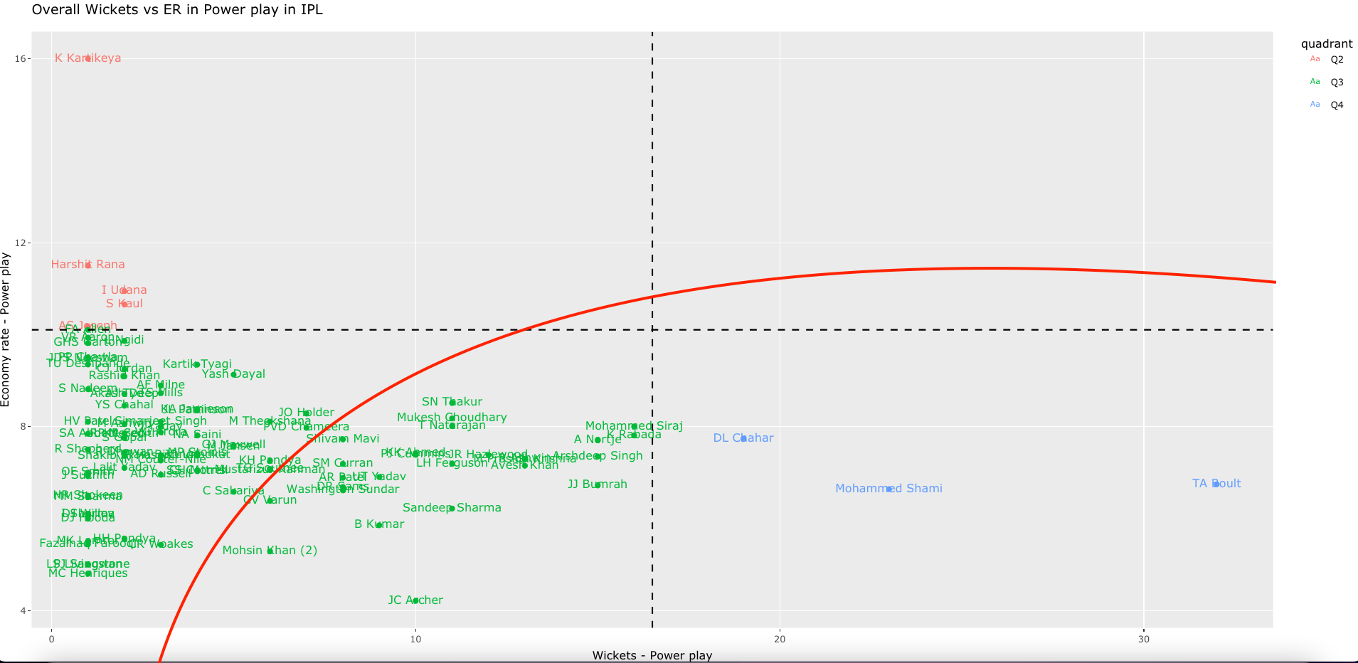
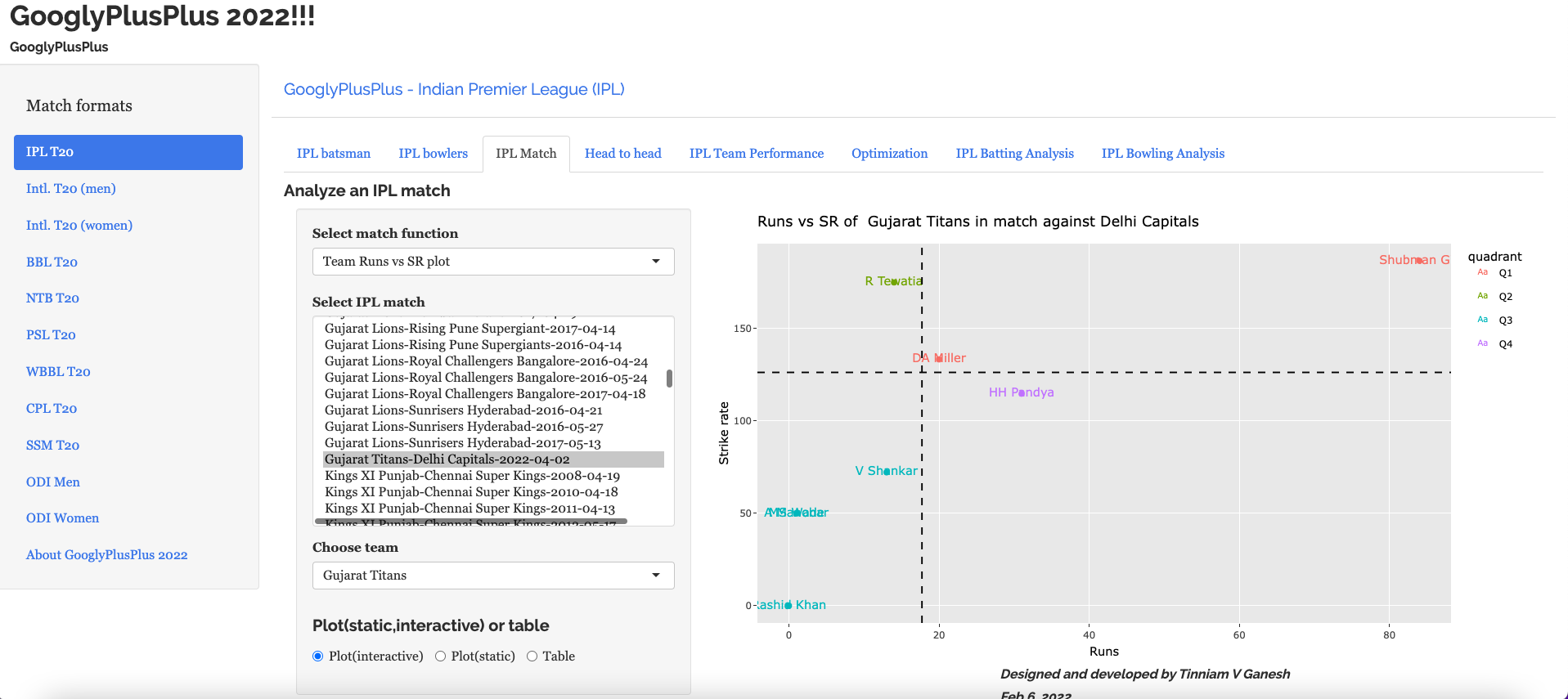
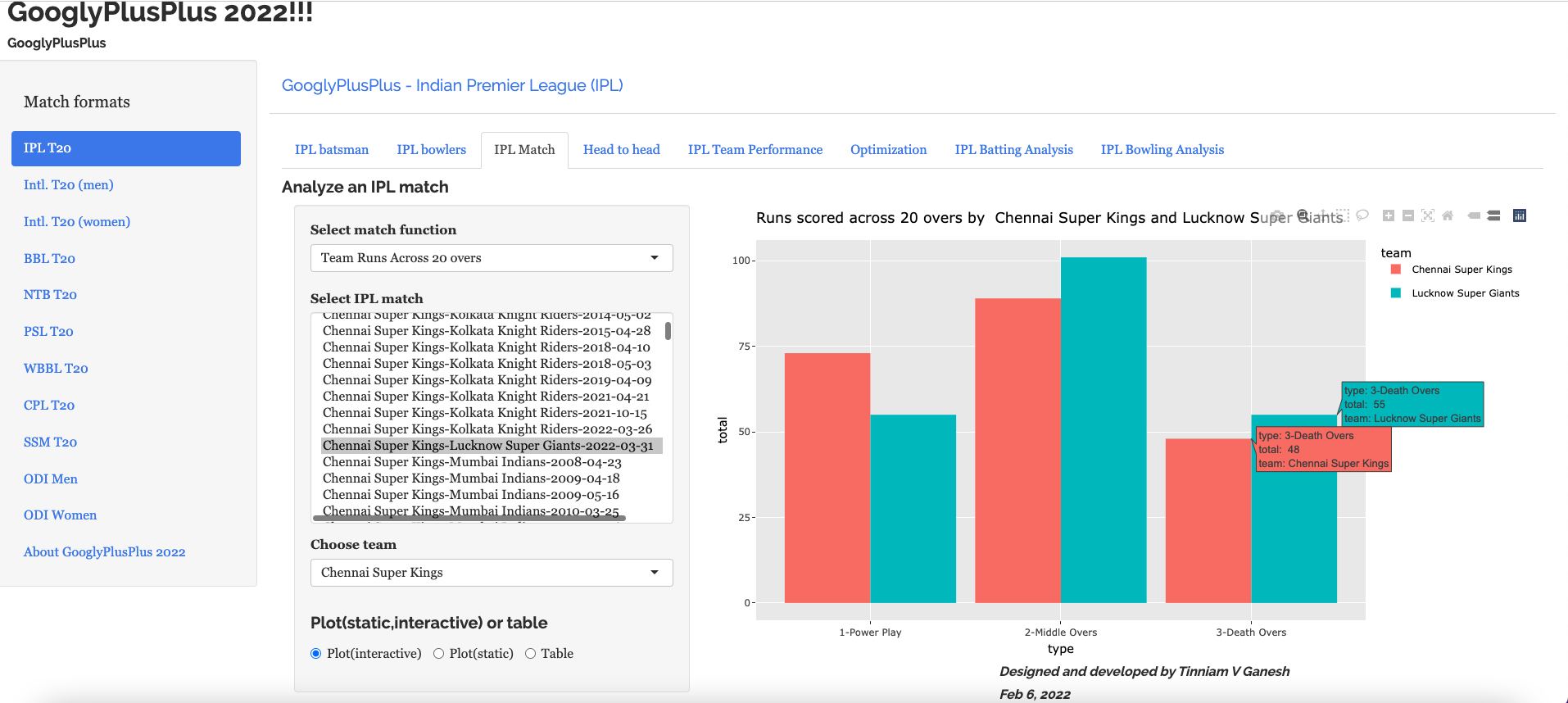
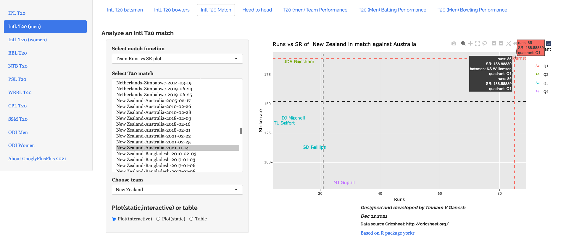
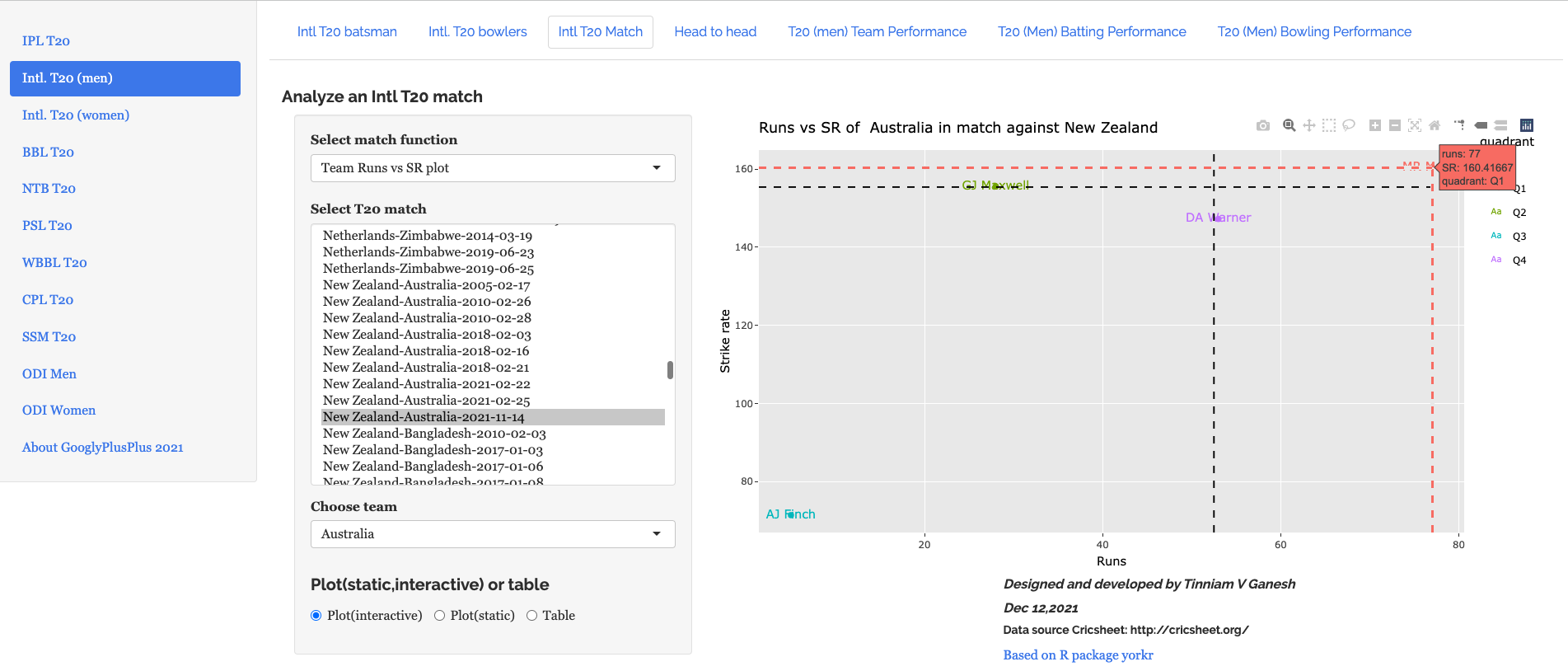
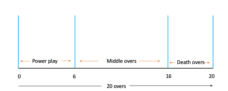
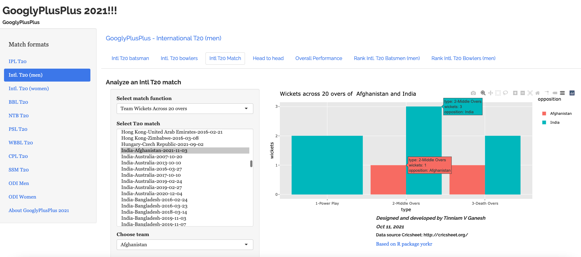
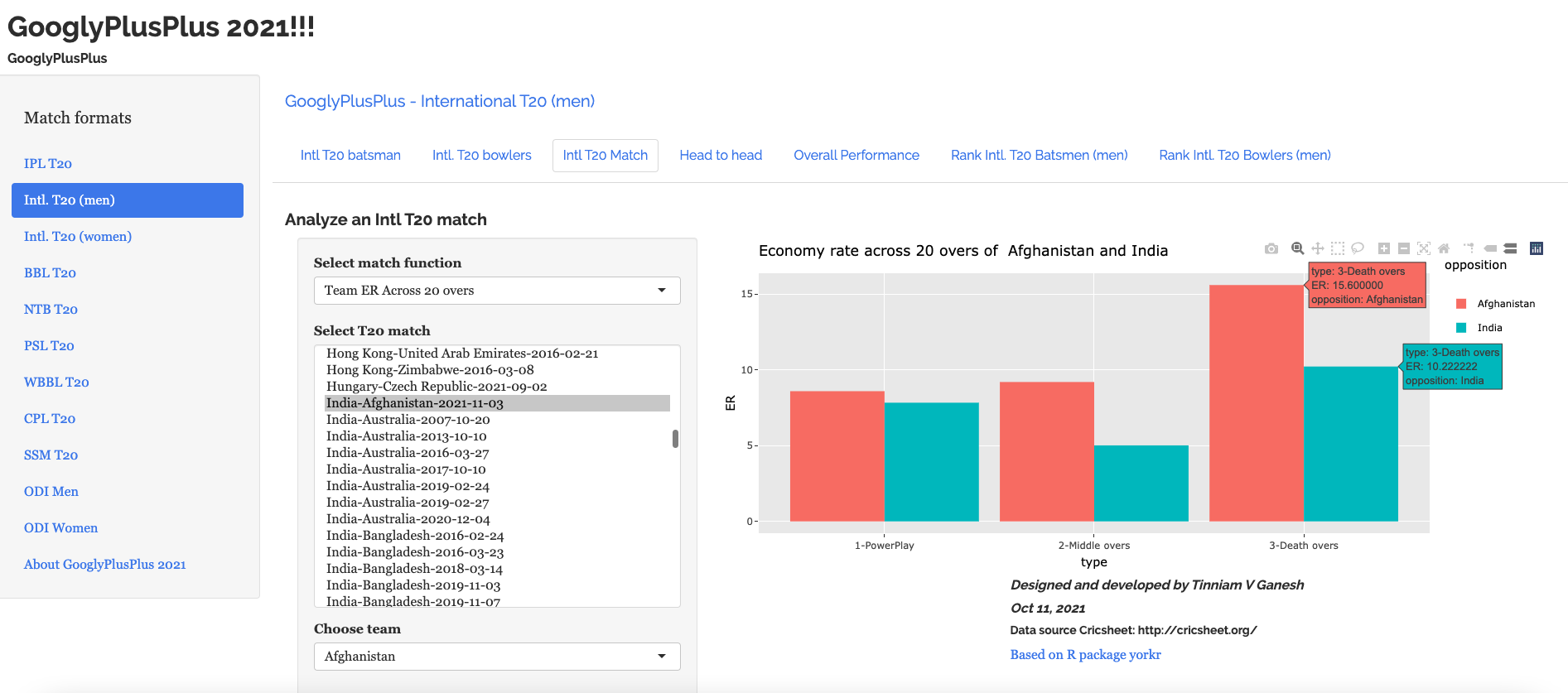
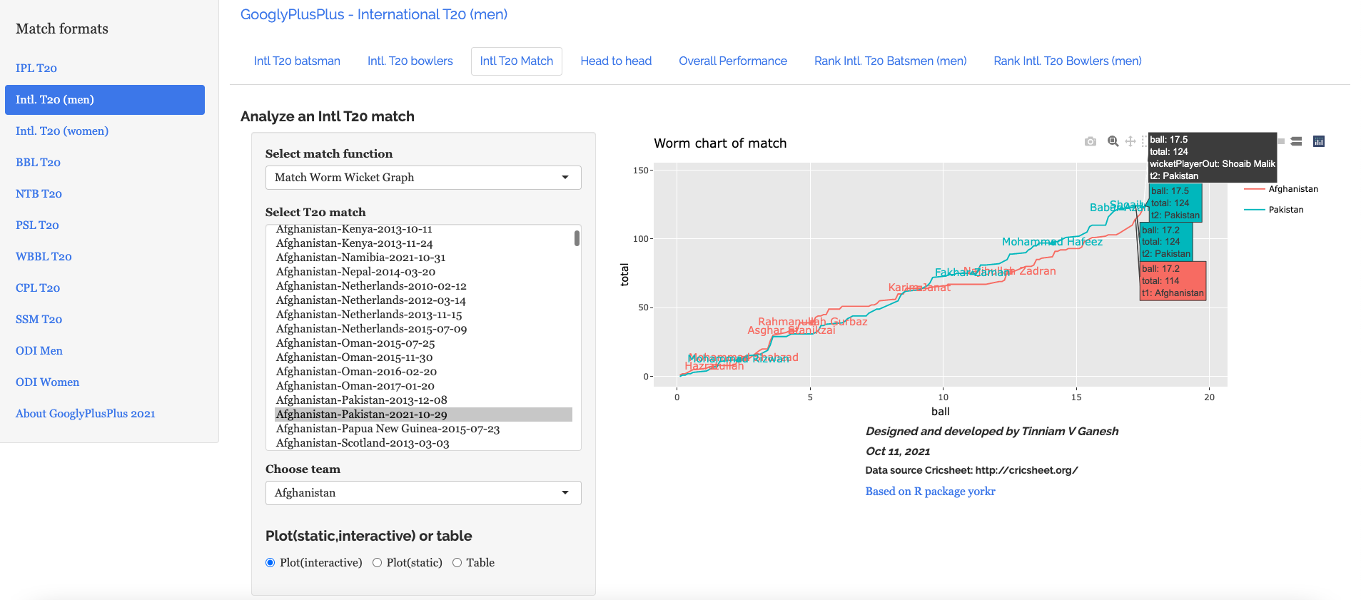
Match tab: Analysis of individual matches, plot of Runs vs SR, Wickets vs ER in power play, middle and death overs, Win Probability Analysis of teams and Win Probability Contribution of players
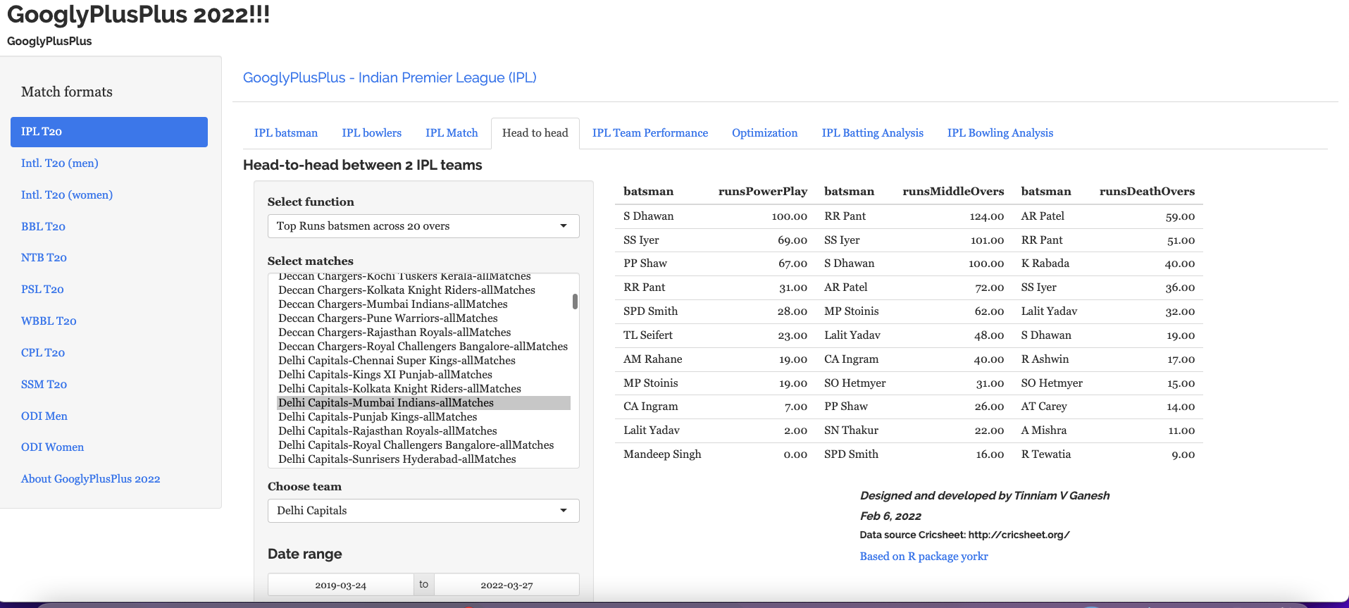
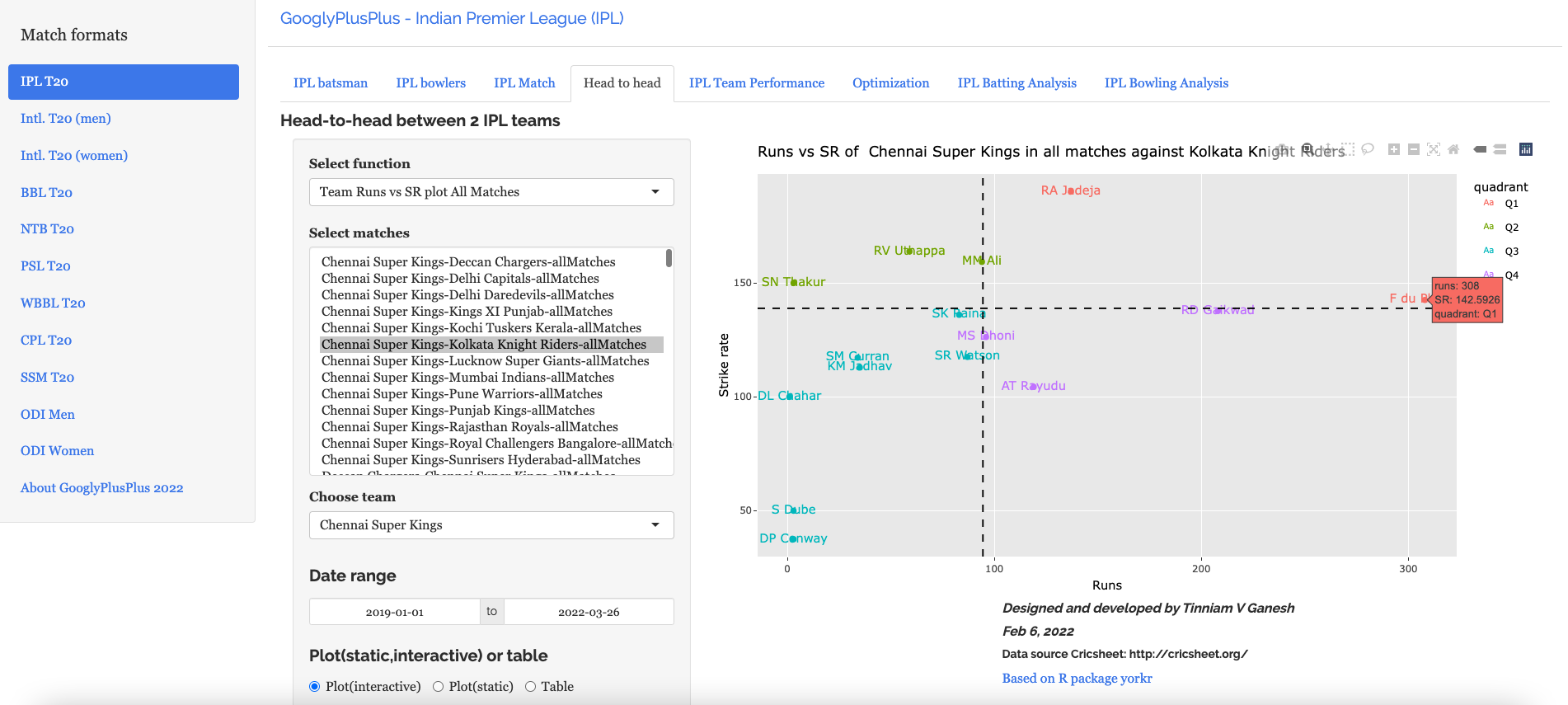
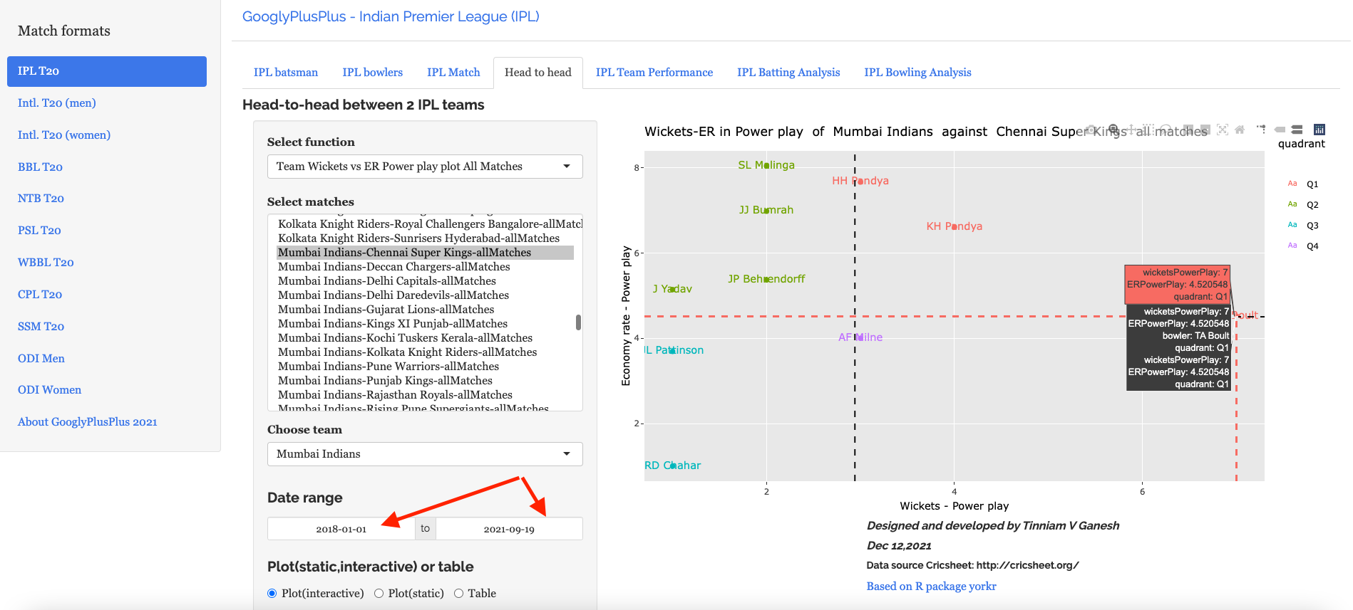
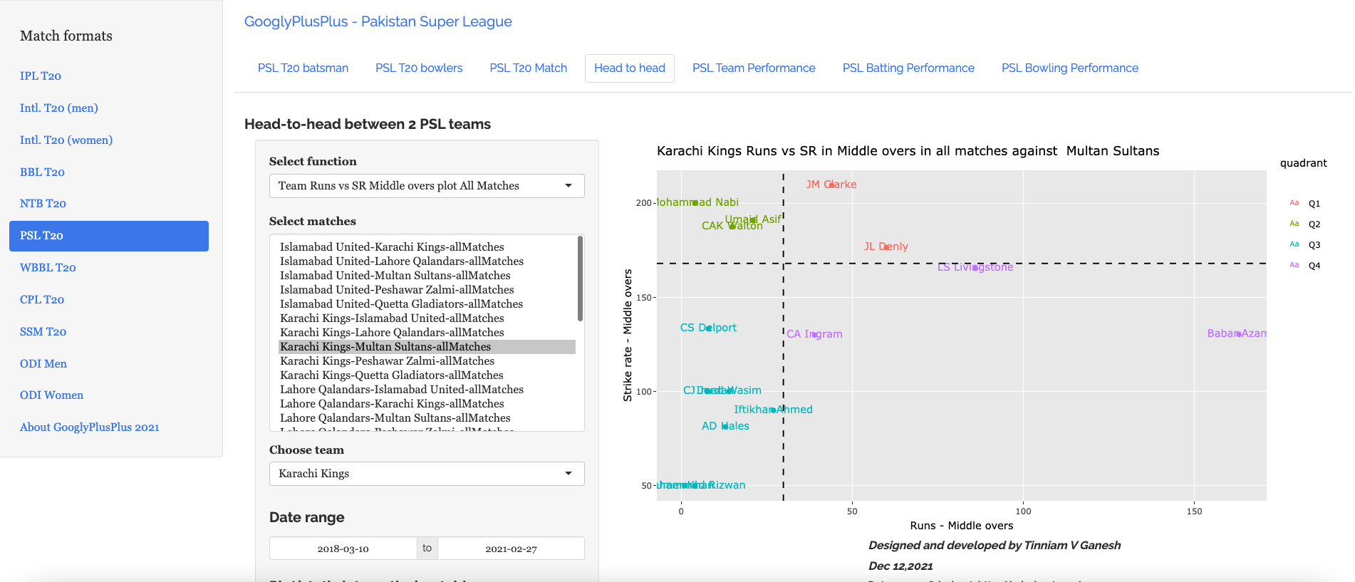
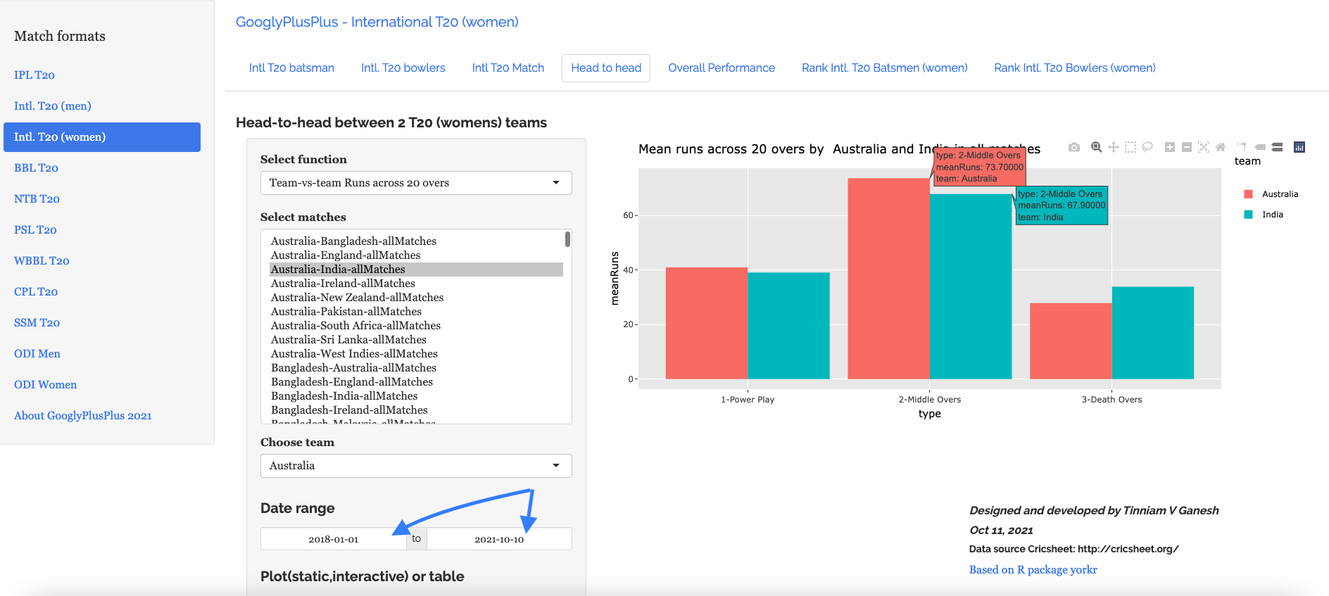
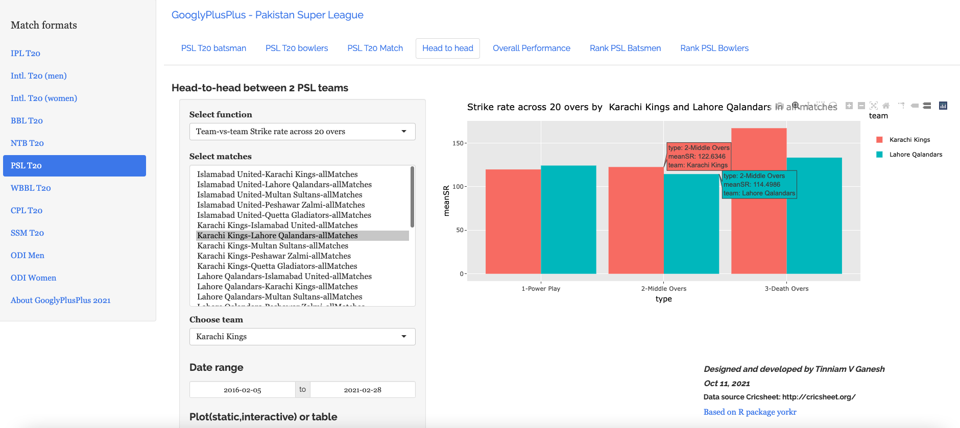
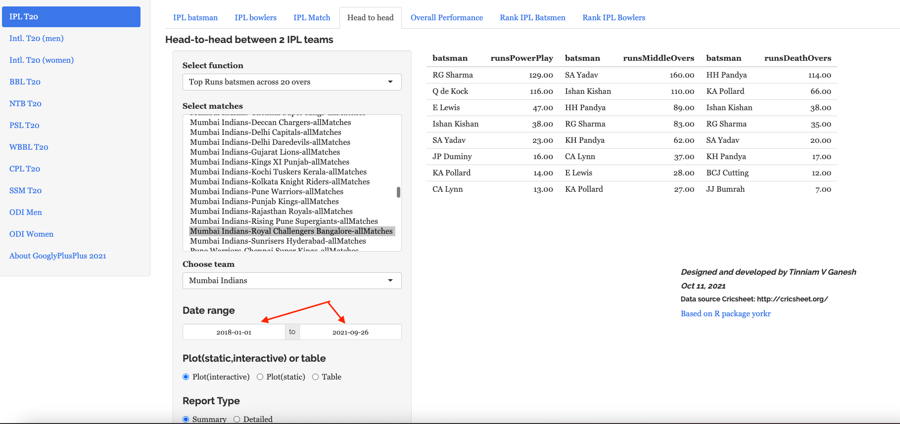
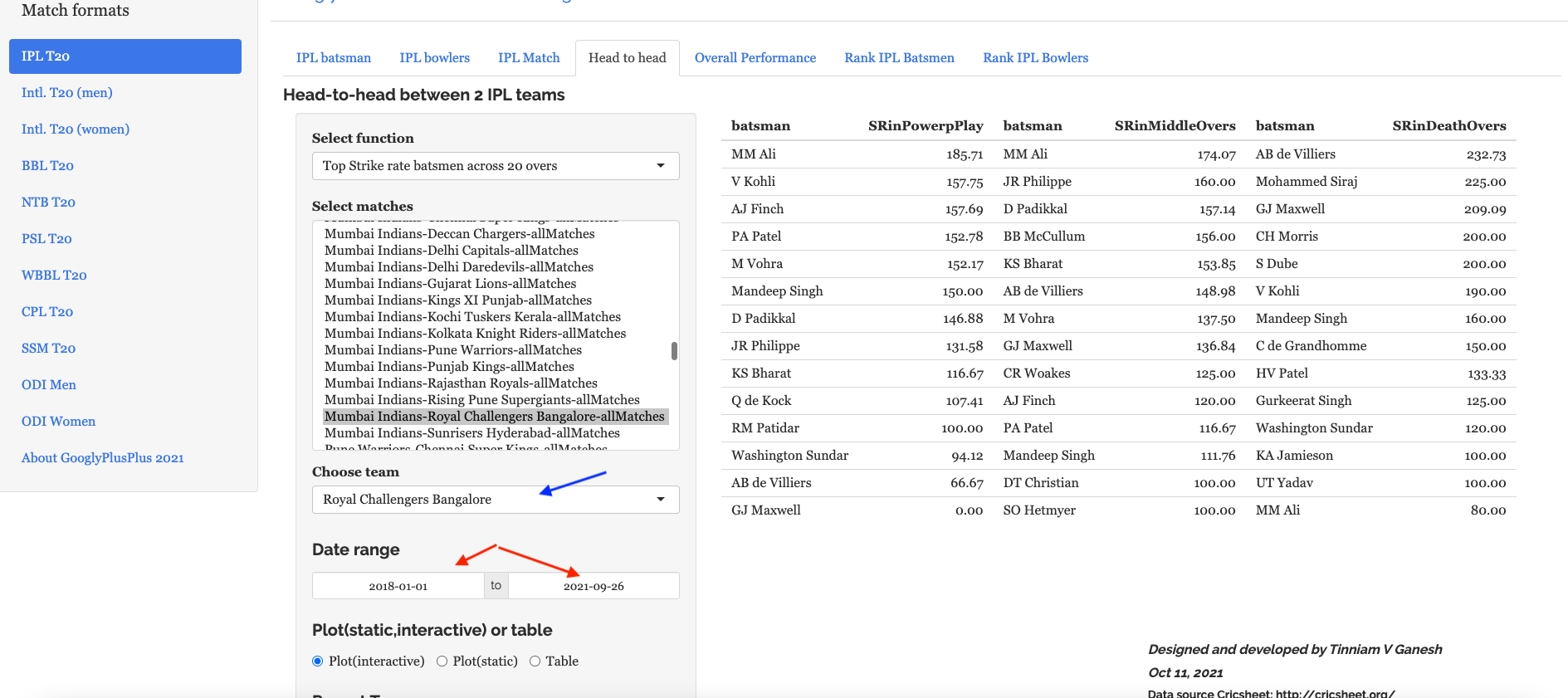
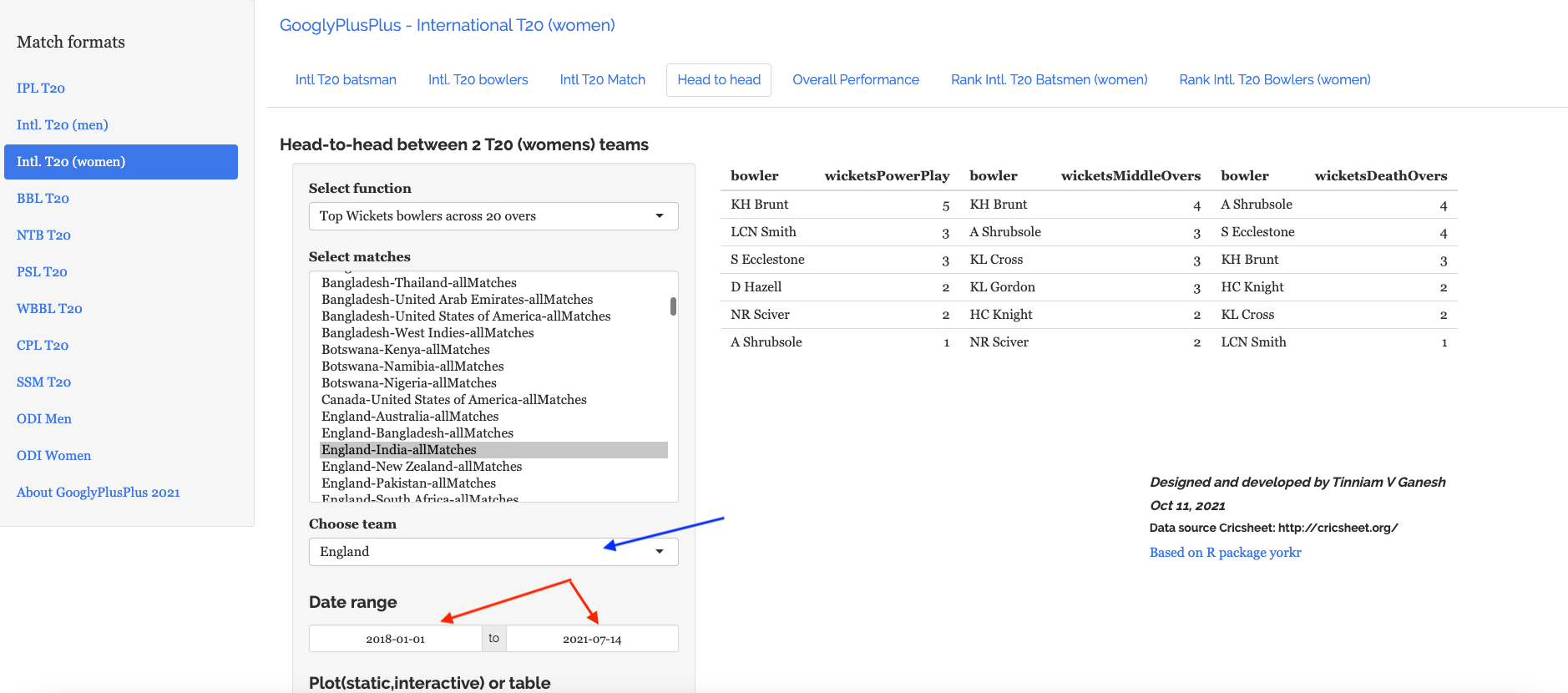
Head-to-head tab: Detailed analysis of team-vs-team batting/bowling scorecard, batting, bowling performances, performances in power play, middle and death overs
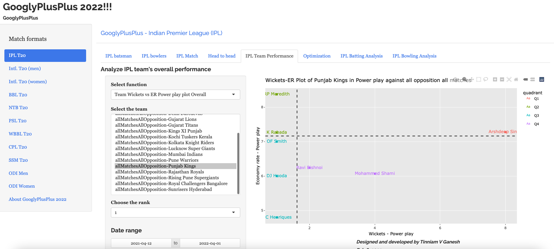
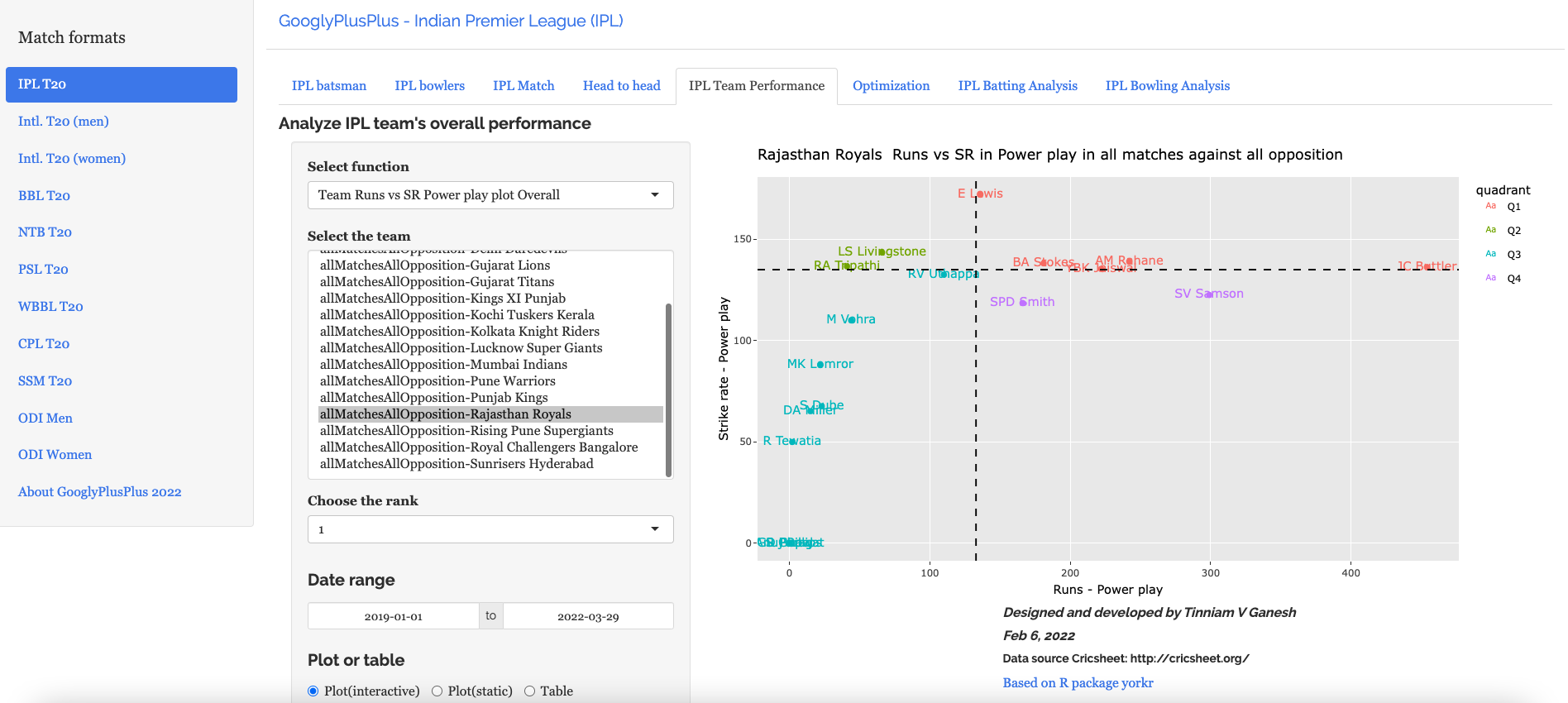
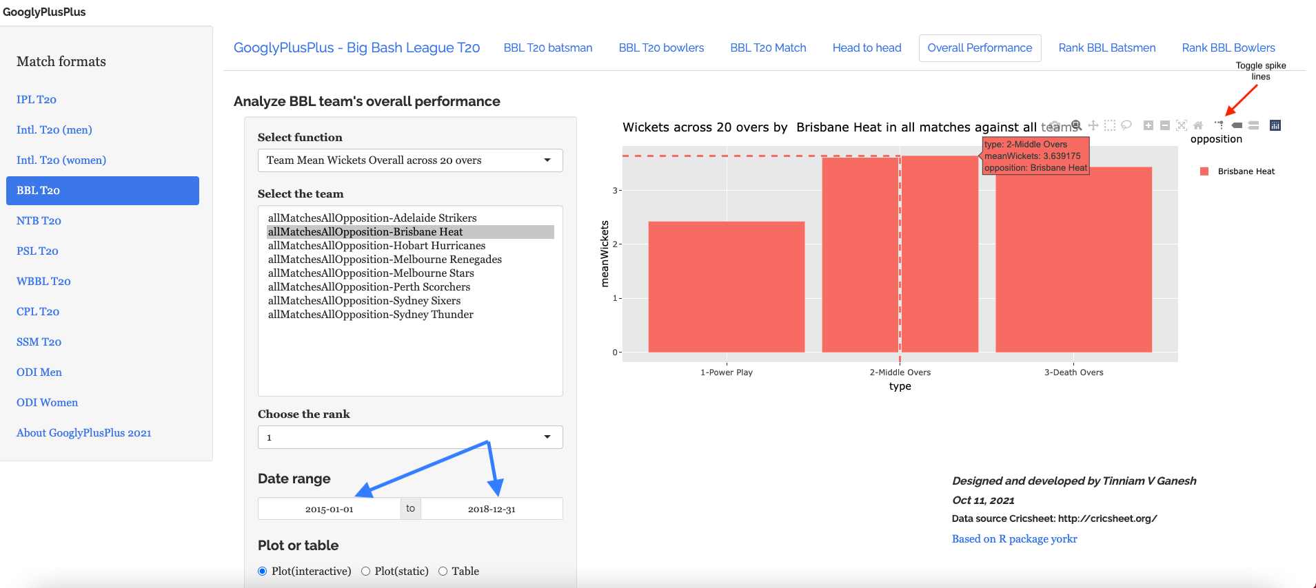
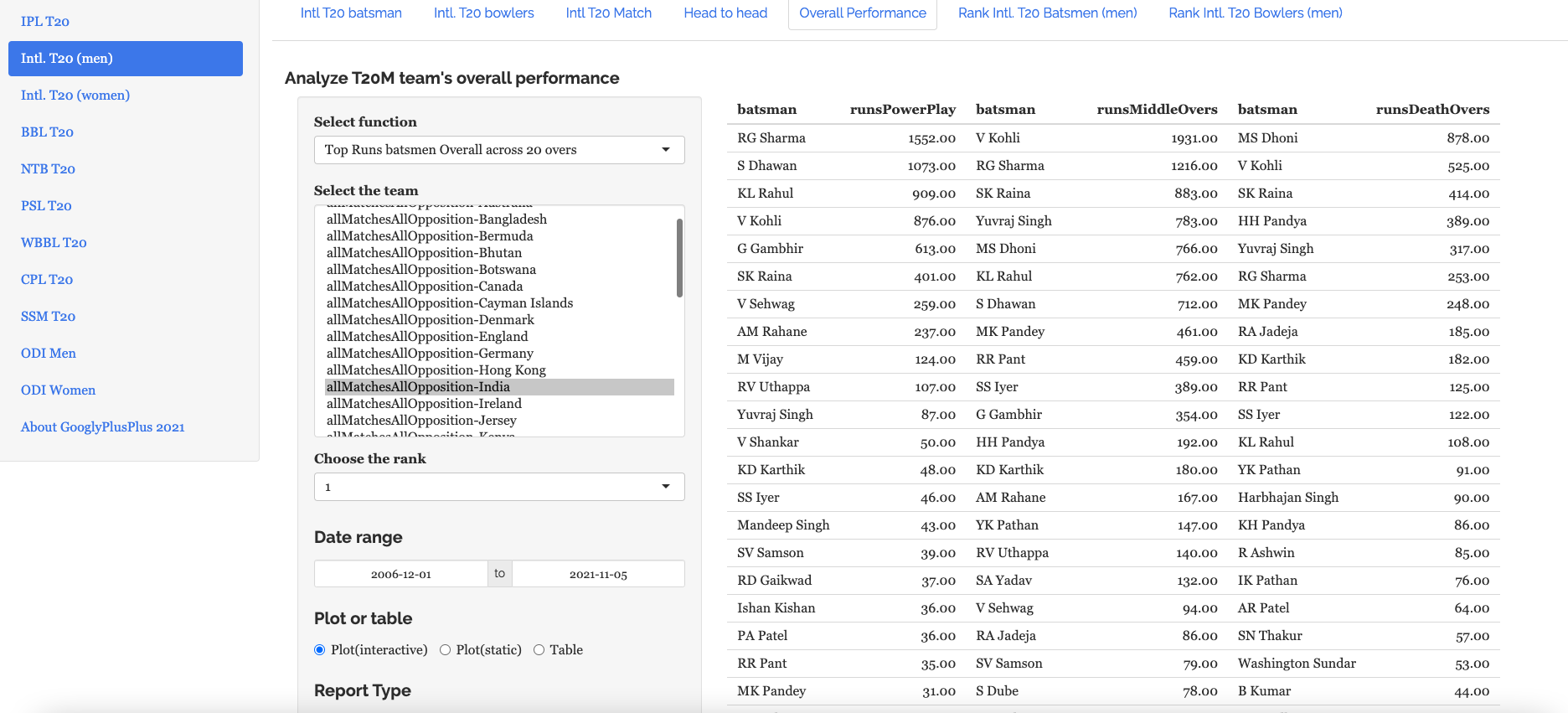
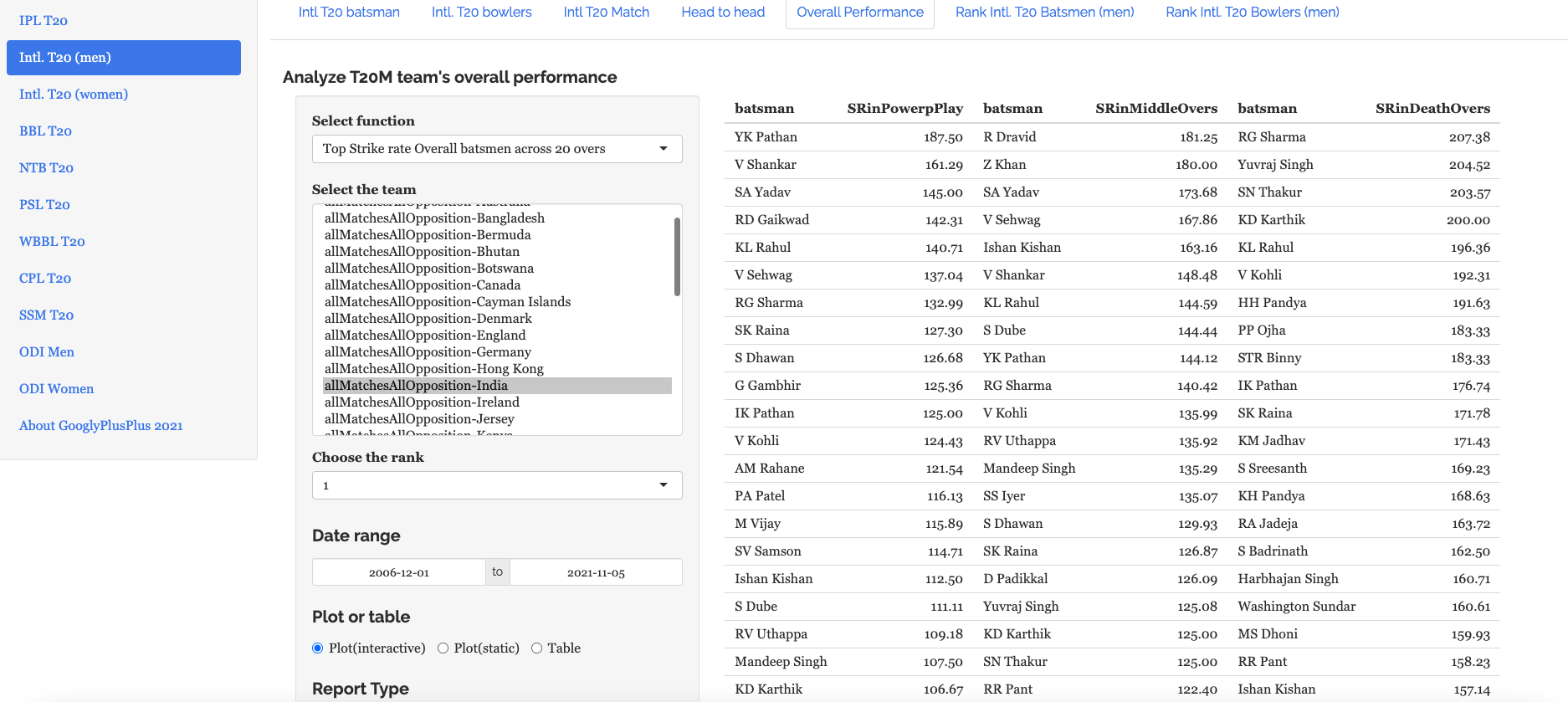
Team performance tab: Analysis of team-vs-all other teams with batting /bowling scorecard, batting, bowling performances, performances in power play, middle and death overs
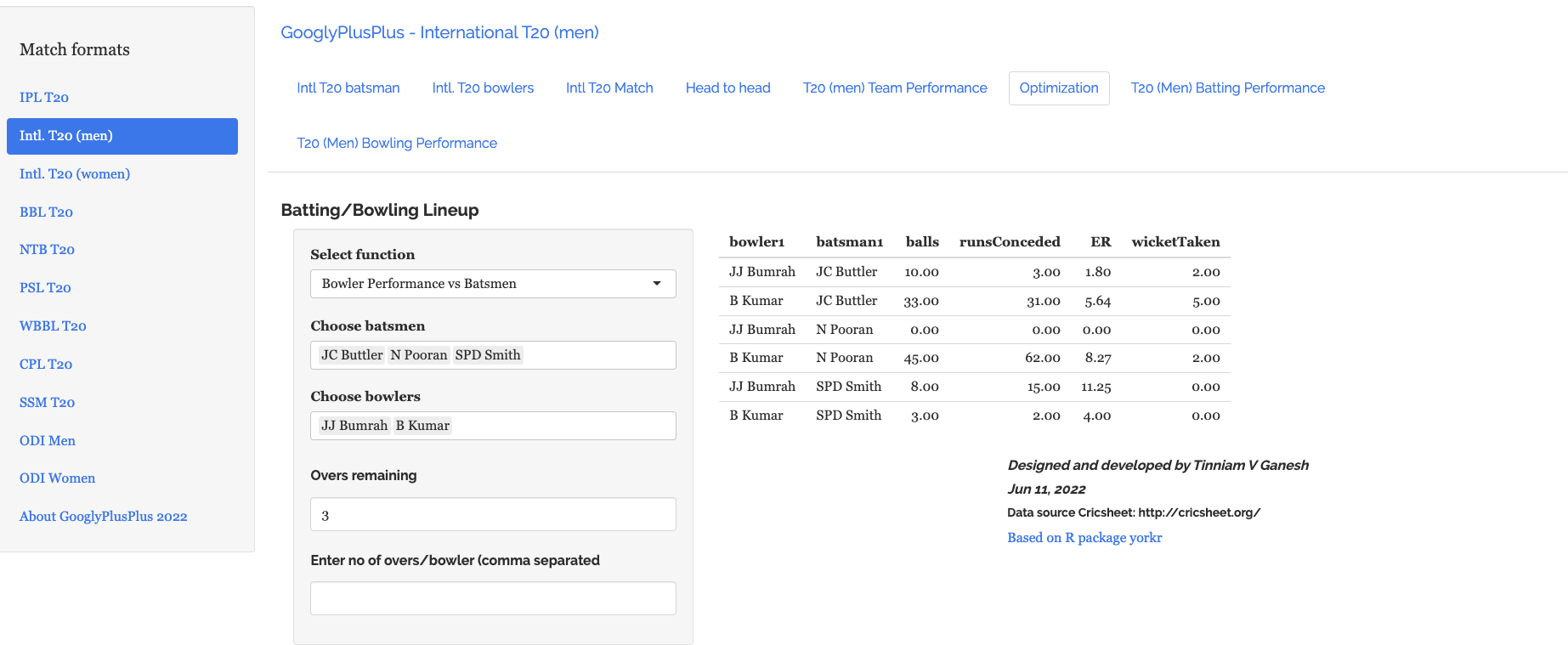
Optimisation tab: Allows one to pit batsmen vs bowlers and vice-versa. This tab also uses integer programming to optimise batting and bowling lineup
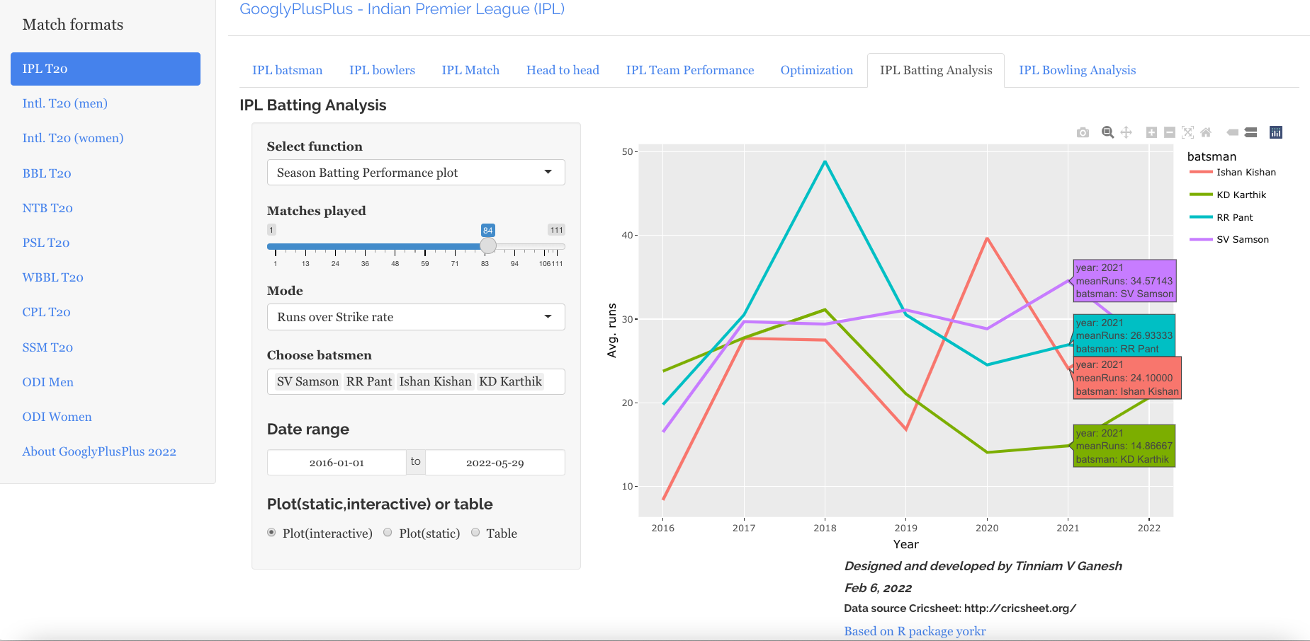
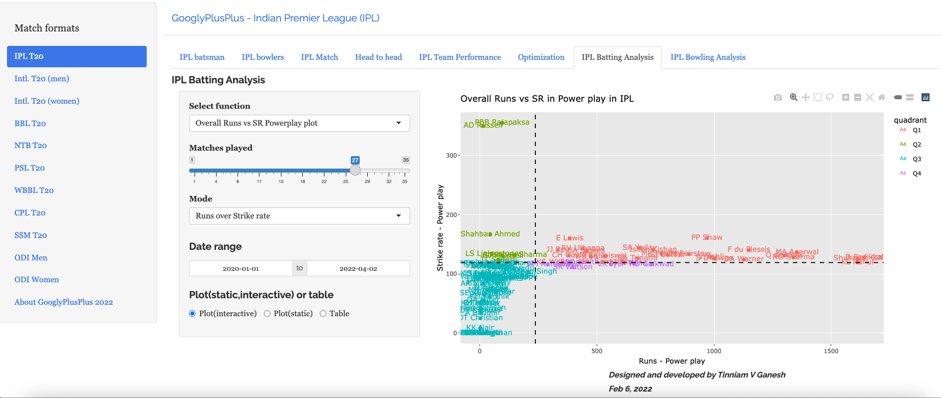
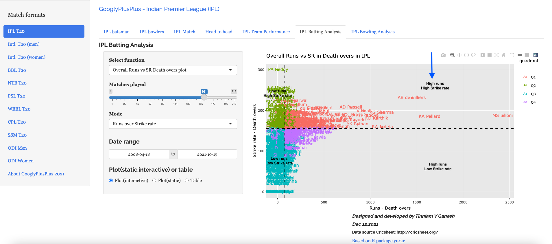
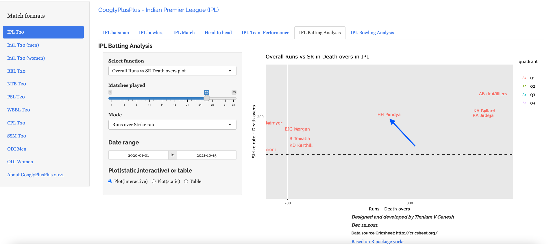
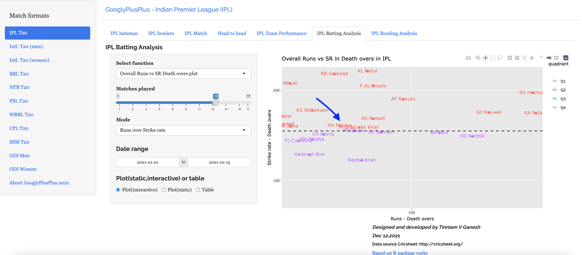
Batting analysis tab: Ranks batsmen using Runs or SR. Also plots performances of batsmen in power play, middle and death overs and plots them in a 4×4 grid
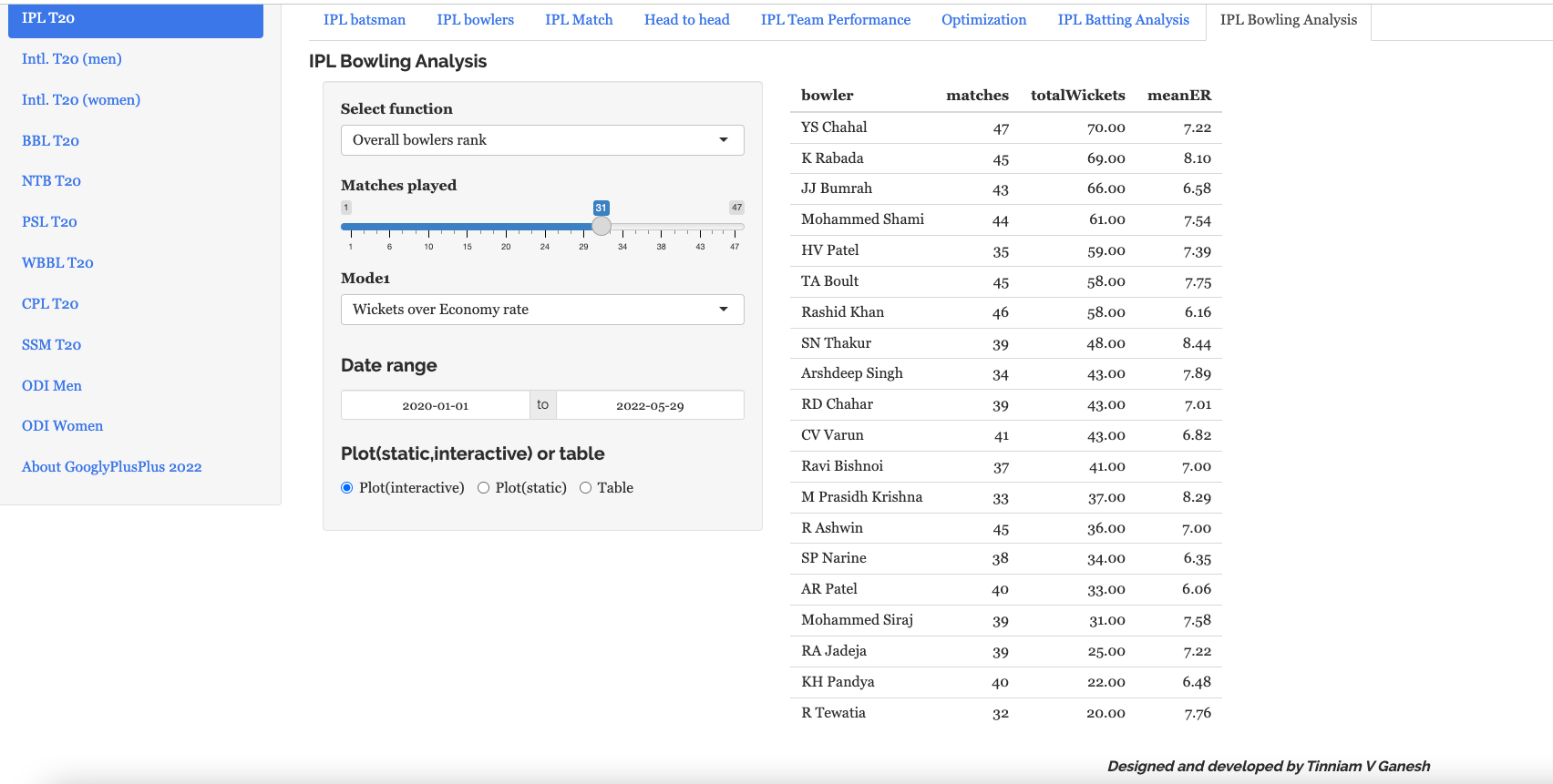
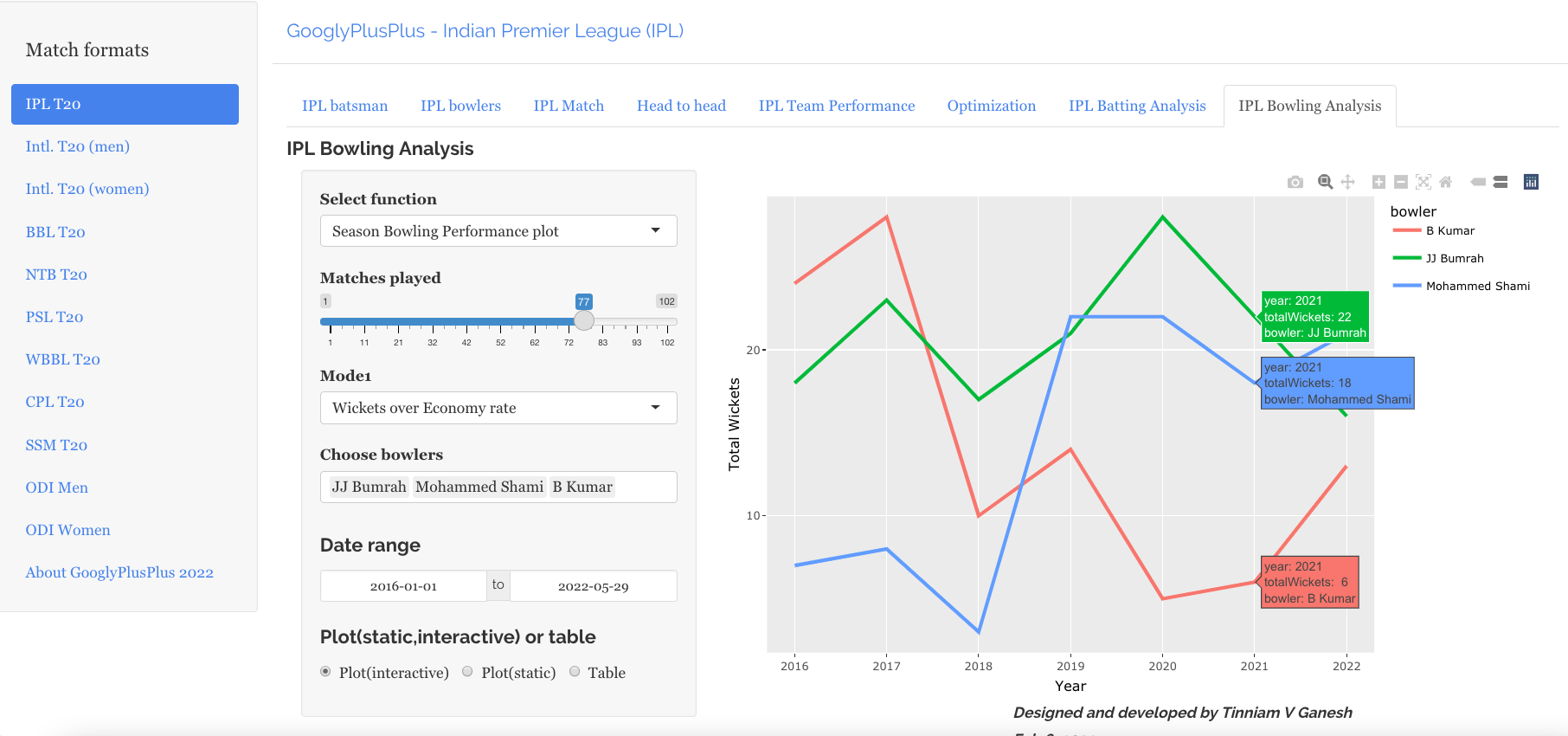
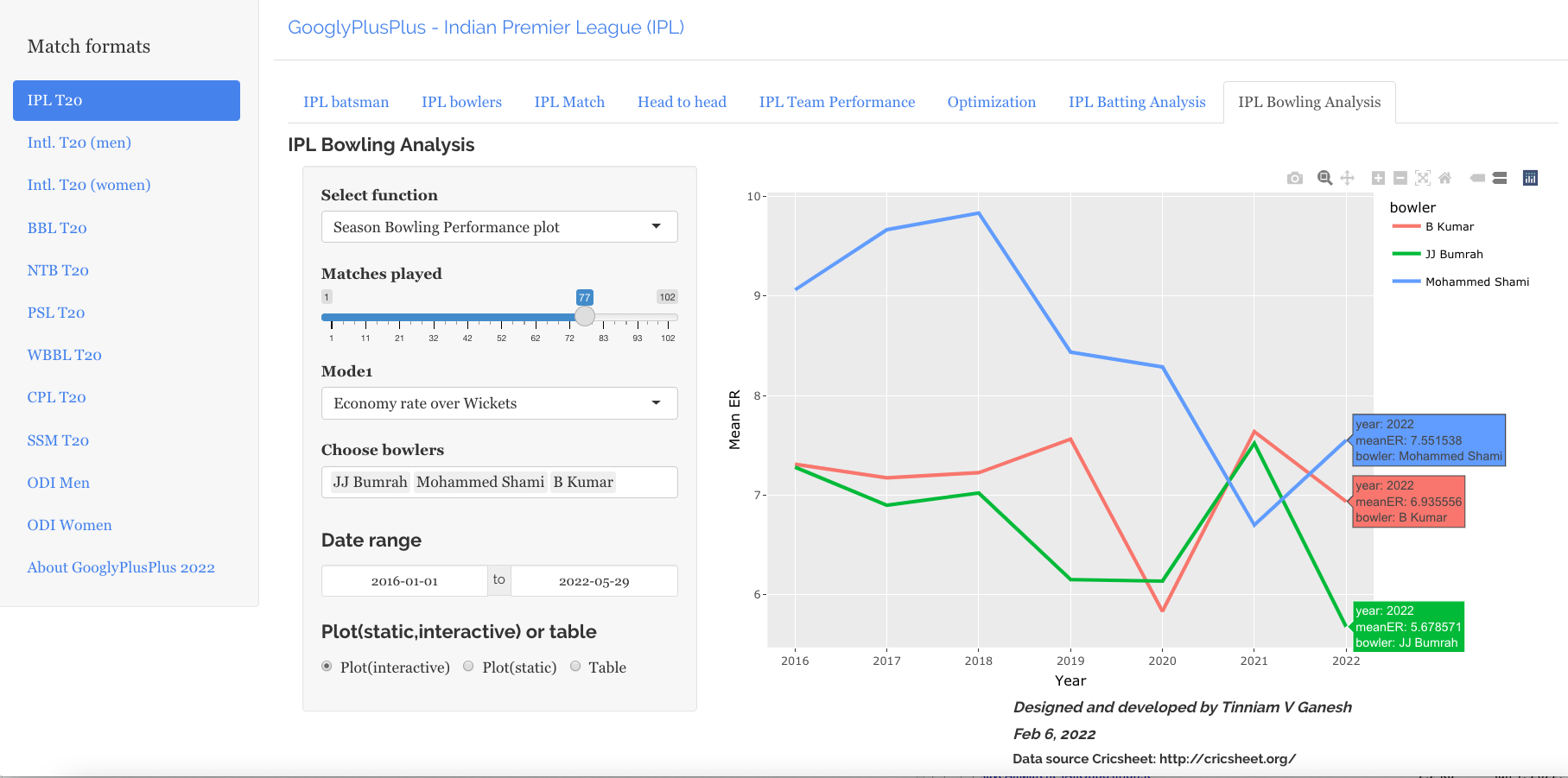
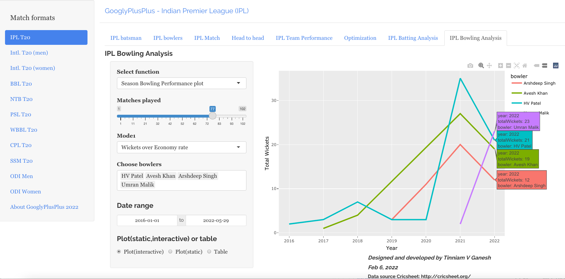
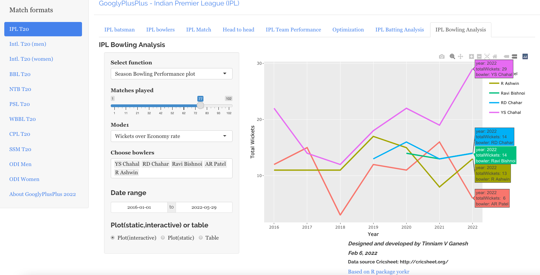
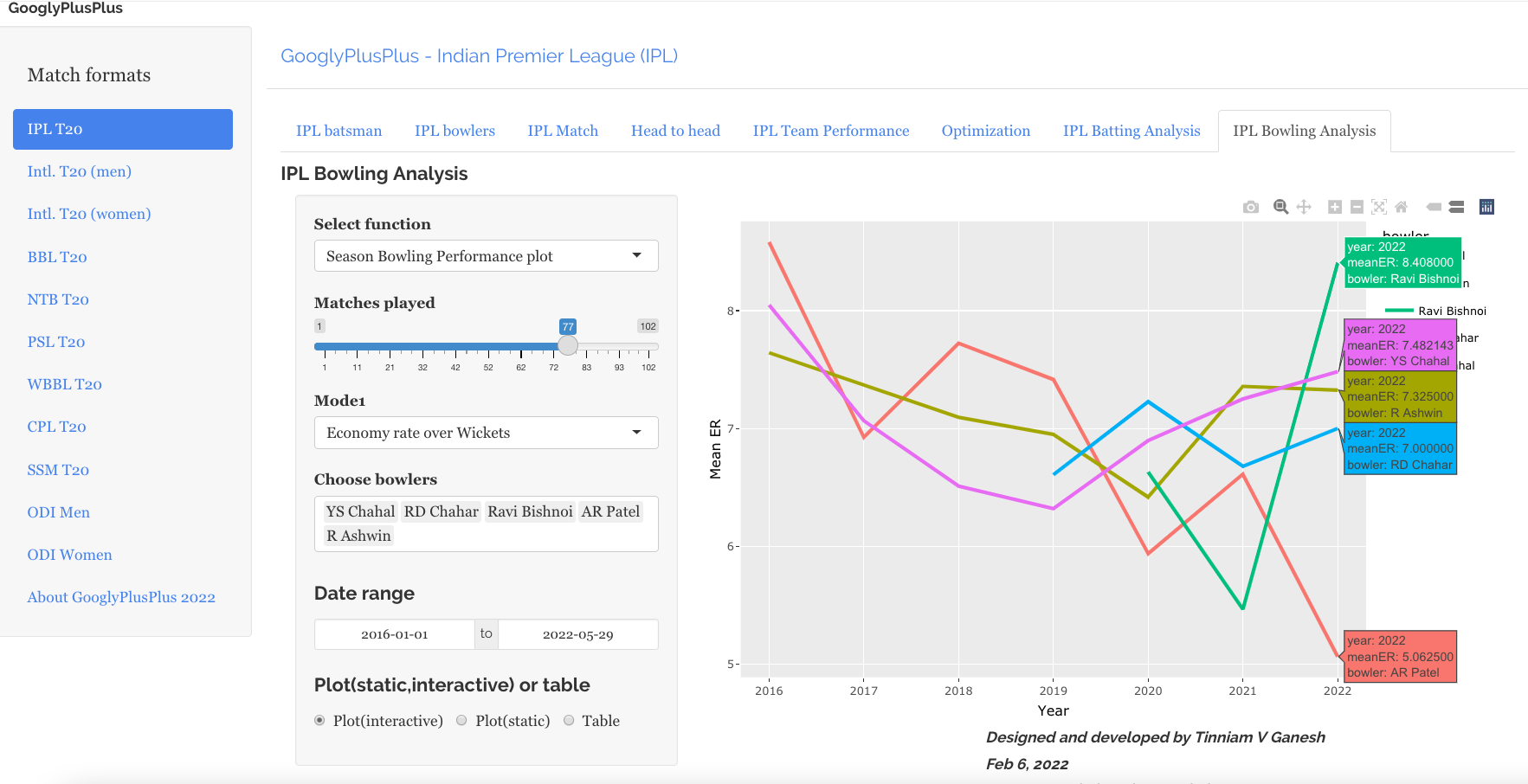
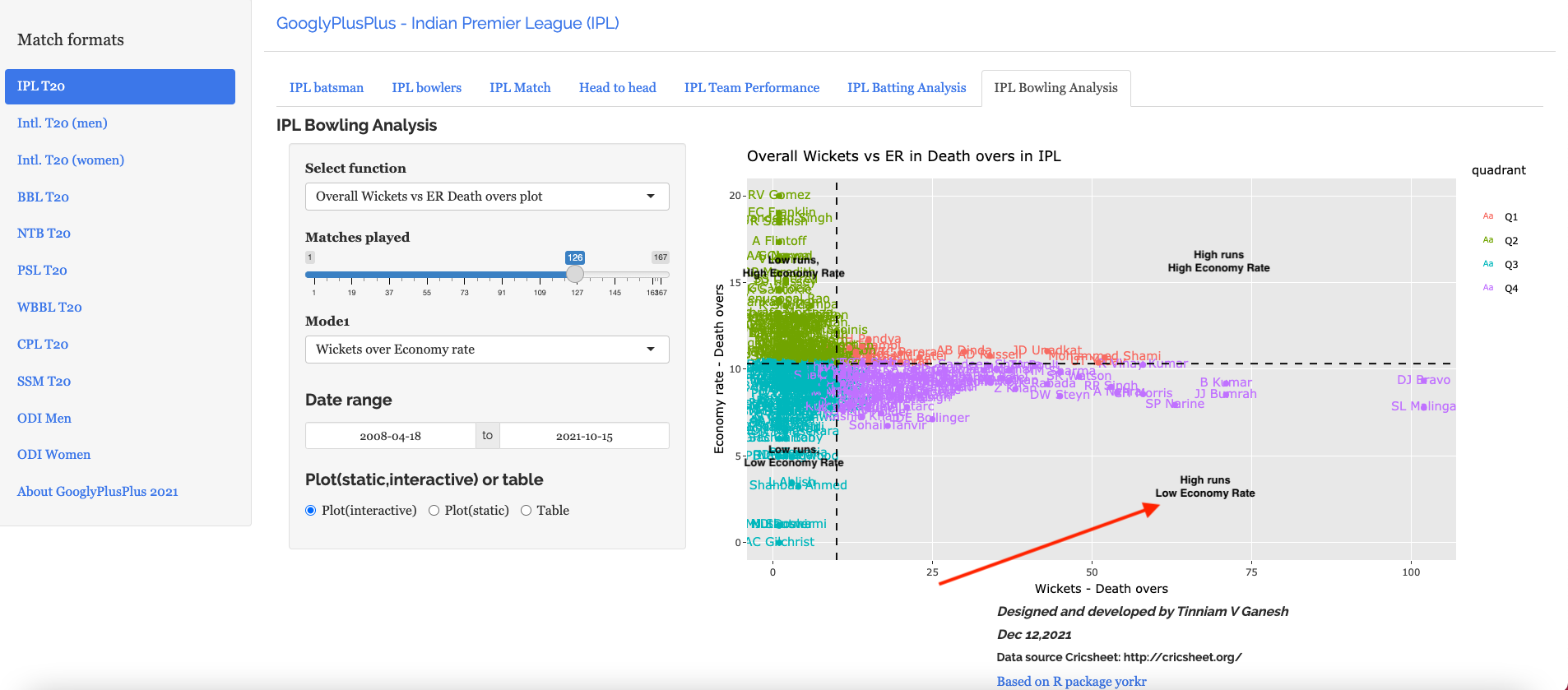
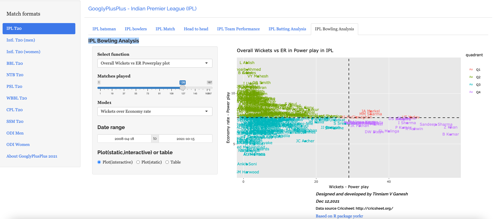
Bowling analysis tab: Ranks bowlers based on Wickets or ER. Also plots performances of bowlers in power play, middle and death overs and plots them in a 4×4 grid
Also note all these tabs and features are available for all T20 formats namely IPL, Intl. T20 (men, women), BBL, NTB, PSL, CPL, SSM.
Important note: It is possible, that at times, the Win Probability (Deep Learning) for some recent IPL matches will give an error. This is because I need to rebuild the models on a daily basis as the matches use player embeddings and there are new players. While I will definitely rebuild the models on weekends and whenever I find time, you may have to bear with this error occasionally.
Note: All charts are interactive, which means that you can hover, zoom-in, zoom-out, pan etc on the charts
The latest avatar of GooglyPlusPlus2023 is based on my R package yorkr with data from Cricsheet.
Follow me on twitter for daily highlights @tvganesh_85
GooglyPlusPlus can analyse players, matches, teams, rank, compute win probability and much more.
Included below are some random analyses of IPL 2023 matches so far
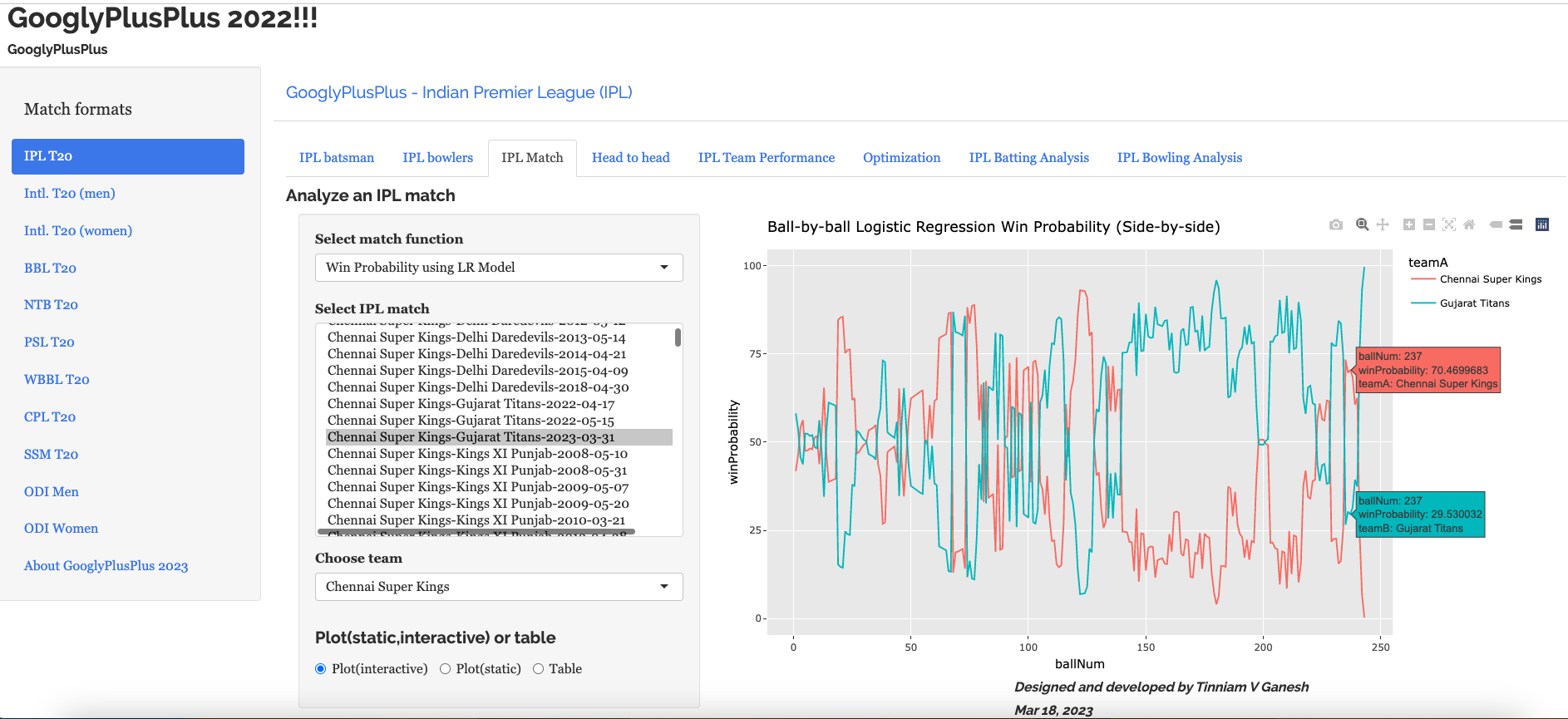
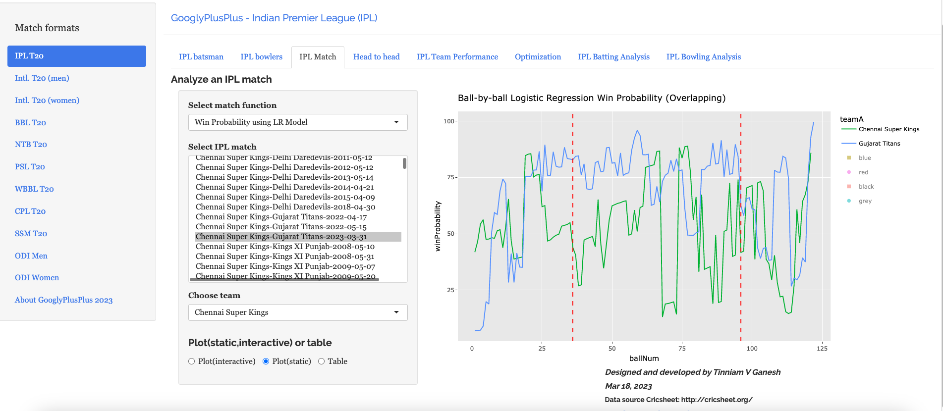
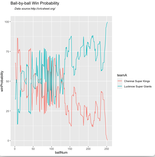
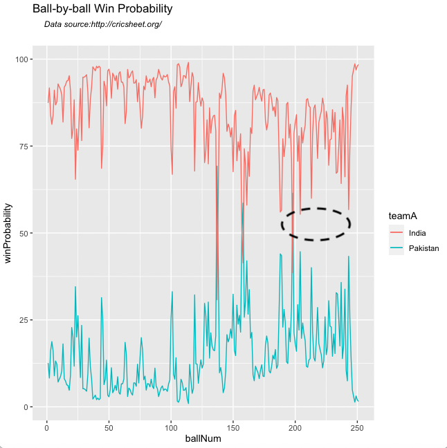
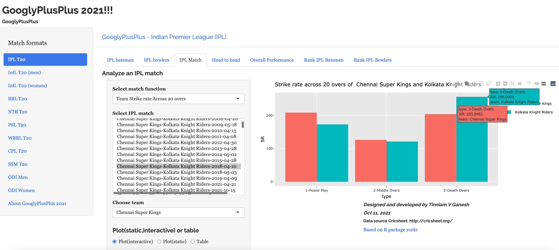
A) Chennai Super Kings vs Gujarat Titans – 31 Mar 2023
GT won by 5 wickets ( 4 balls remaining)
a) Worm Wicket Chart
b) Ball-by-ball Win Probability (Logistic Regression) (side-by-side)
This model shows that CSK had the upper hand in the 2nd last over, before it changed to GT. More details on Win Probability and Win Probability Contribution in the posts given by the links above.
c) b) Ball-by-ball Win Probability (Logistic Regression) (overlapping)
Here the ball-by-ball win probability is overlapped. CSK and GT both had nearly the same probability of winning in the 2nd last over before GT edges CSK out
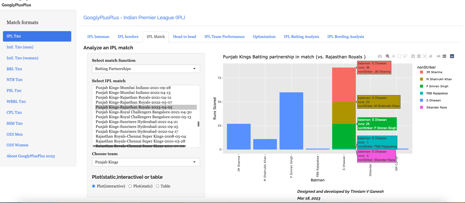
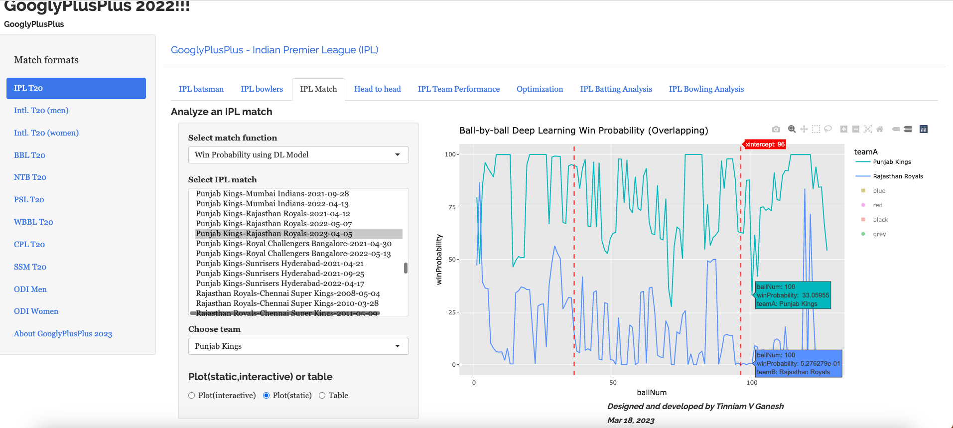
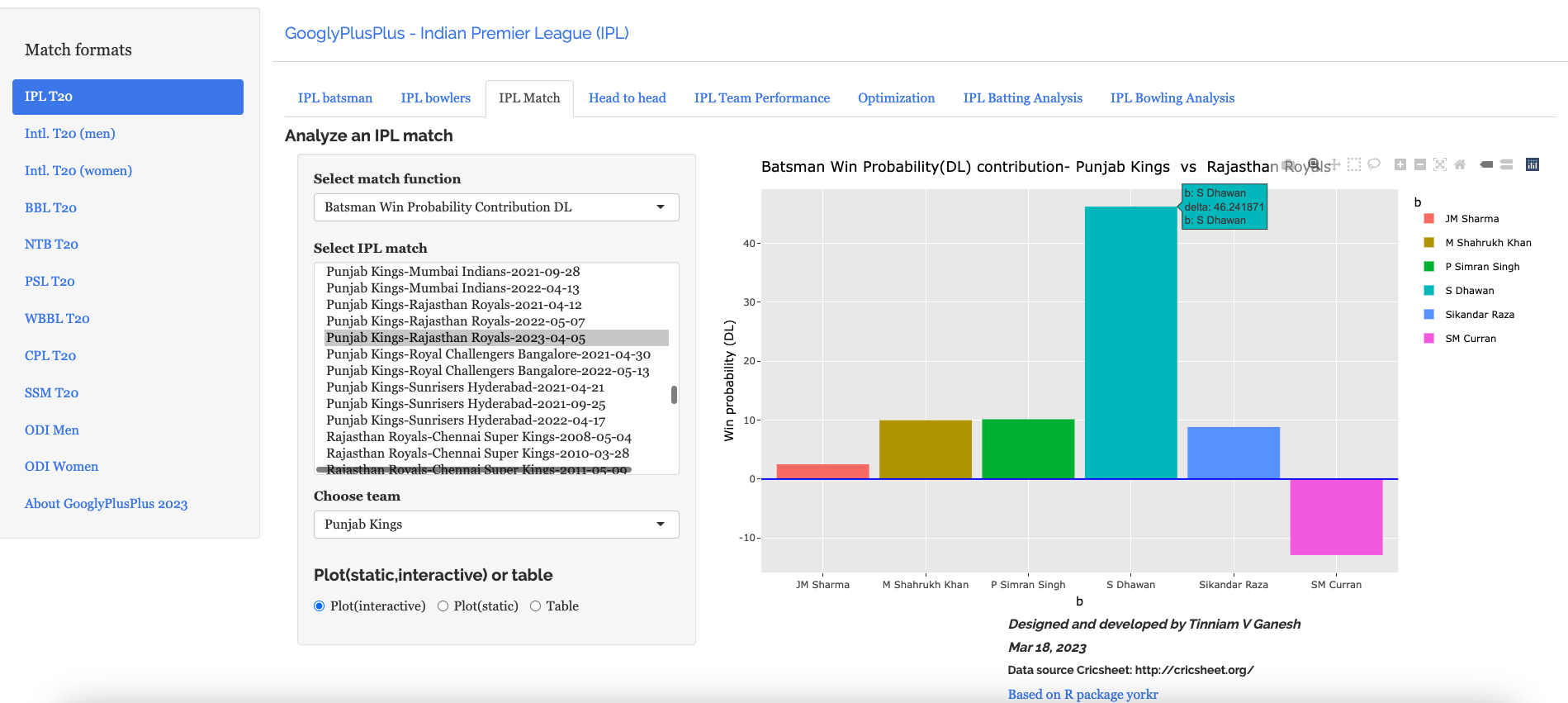
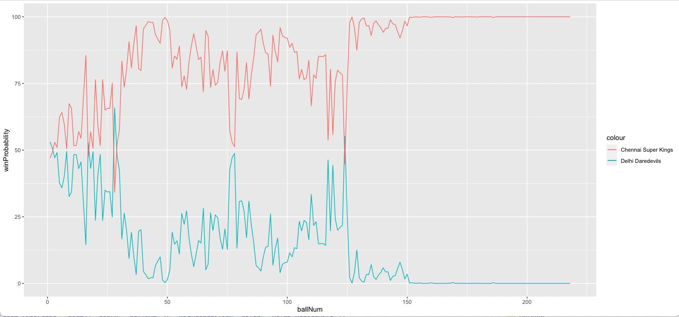
B) Punjab Kings vs Rajasthan Royals – 05 Apr 2023
This was a another closely fought match. PBKS won by 5 runs
a) Worm wicket chart
b) Batting partnerships
Shikhar Dhawan scored 86 runs
c) Ball-by-ball Win Probability using Deep Learning (overlapping)
PBKS was generally ahead in the win probability race
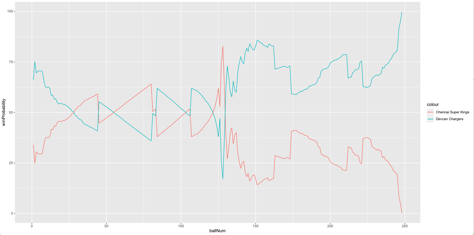
d) Batsman Win Probability Contribution
This plot shows how the different batsmen contributed to the Win Probability. We can see that Shikhar Dhawan has a highest win probability. He played a very sensible innings. Also it appears that there is no difference between Prabhsimran Singh and others, though he score 60 runs. This computation is based on when they come to bat and how the win probability changes when they get dismissed, as seen in the 2nd chart
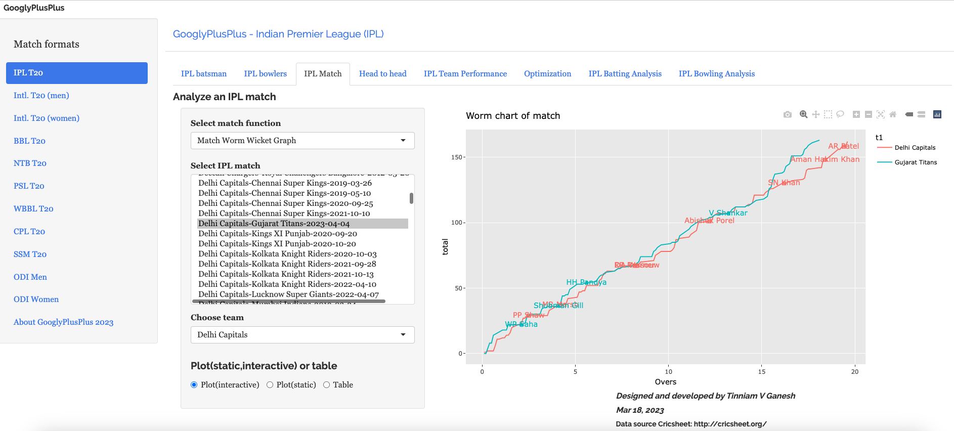
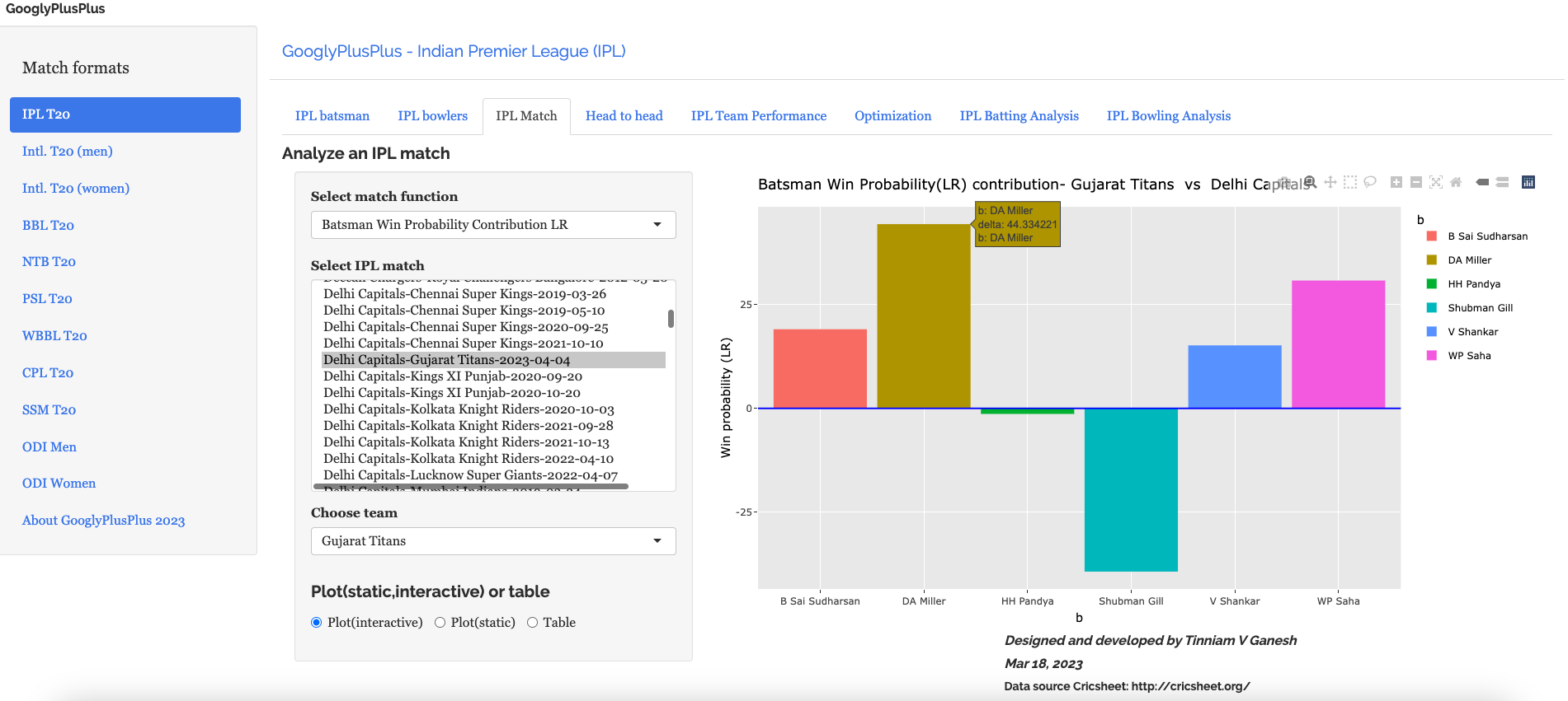
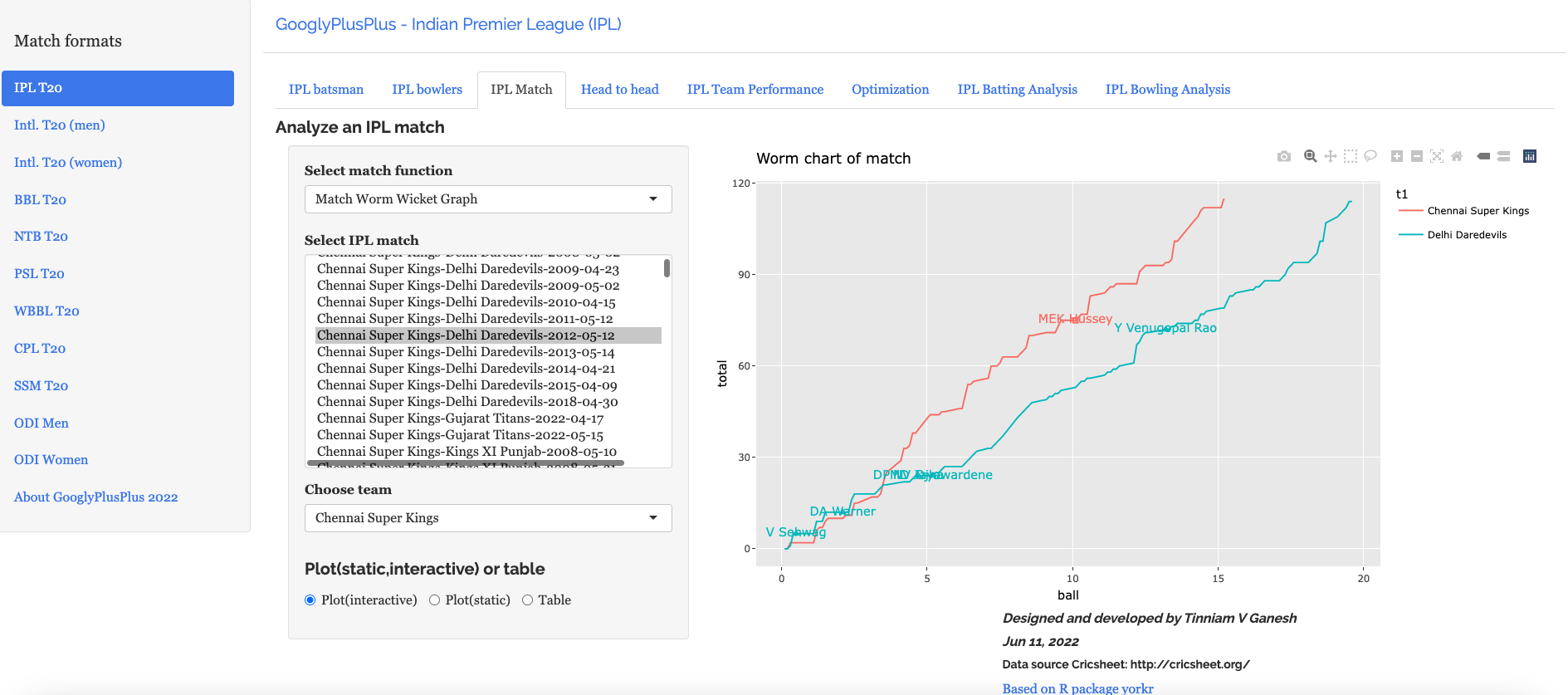
C) Delhi Capitals vs Gujarat Titans – 4 Apr 2023
GT won by 6 wickets (11 balls remaining)
a) Worm wicket chart
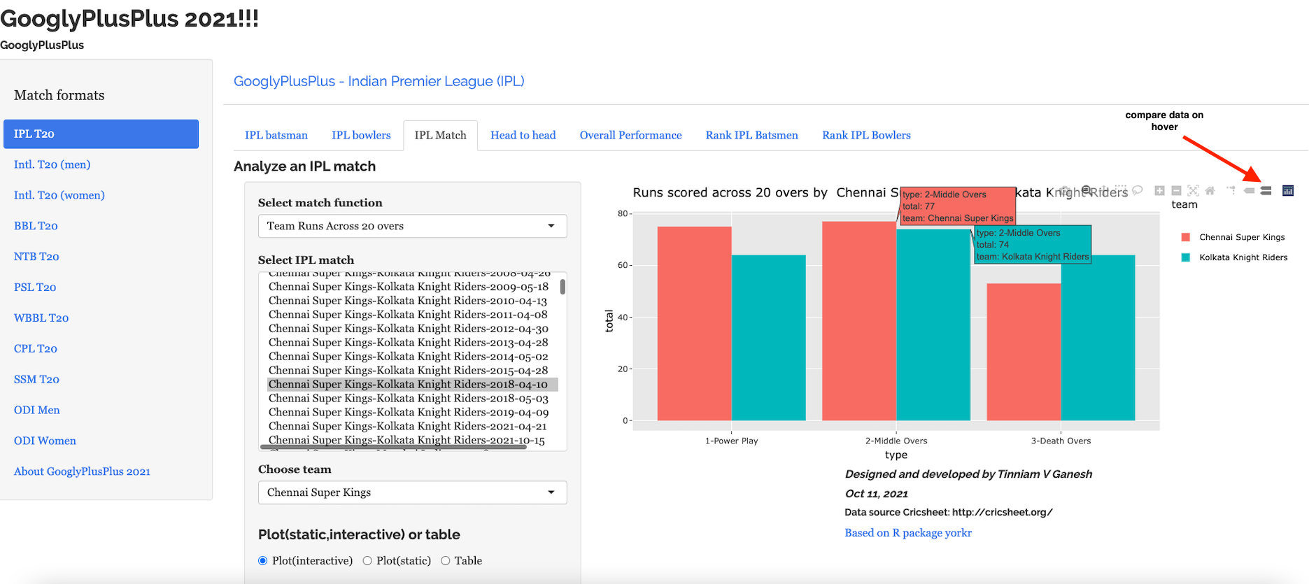
b) Runs scored across 20 overs
c) Runs vs SR plot
d) Batting scorecard (Gujarat Titans)
e) Batsman Win Probability Contribution (Gujarat Titans)
Miller has a higher percentage in the Win Contribution than Sai Sudershan who held the innings together.Strange are the ways of the ML models!!
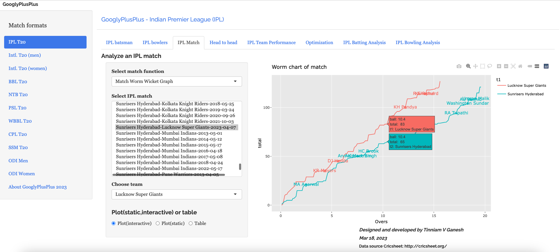
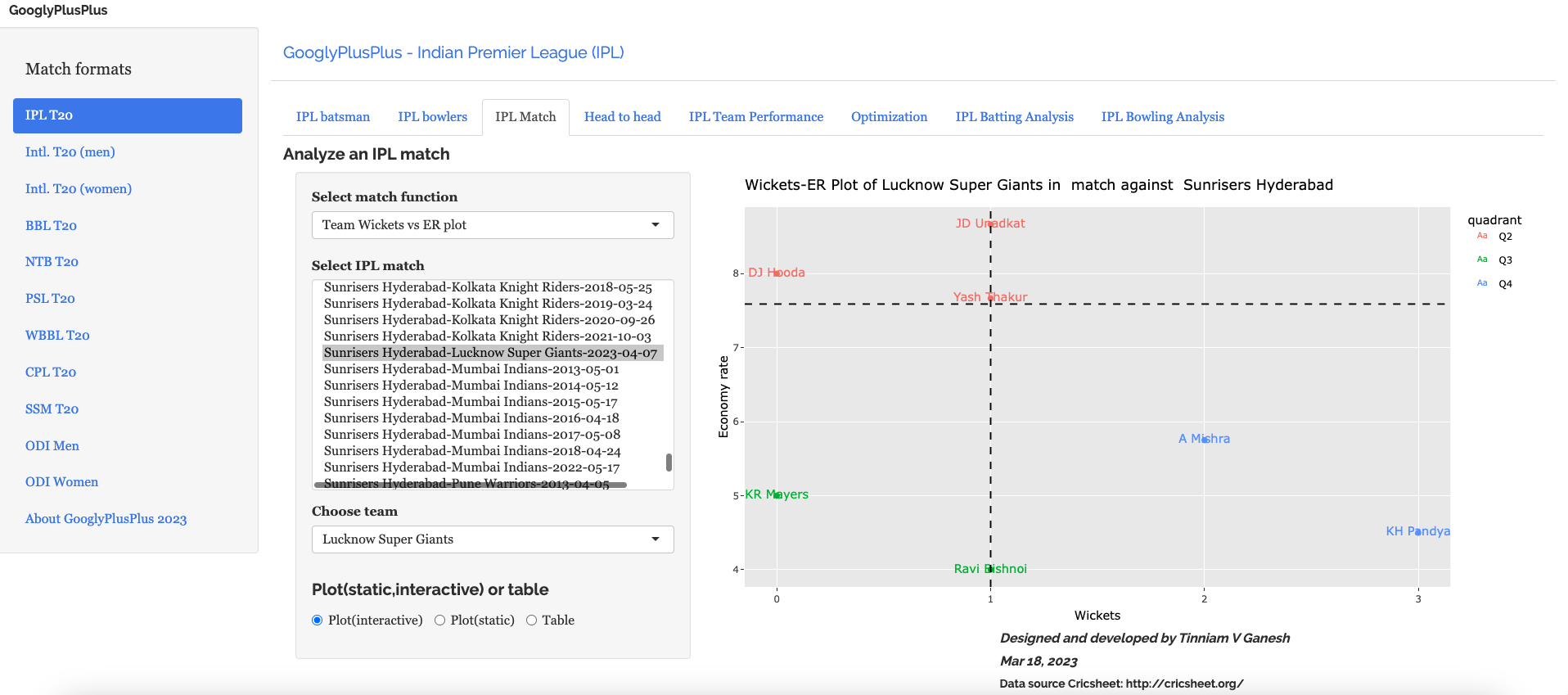
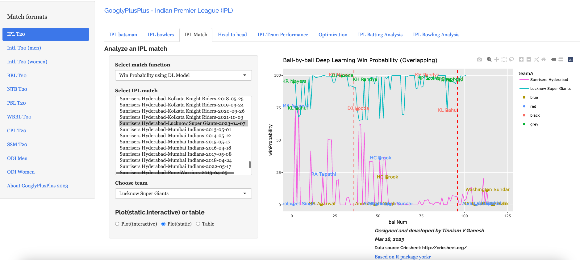
D) Sunrisers Hyderabad vs Lucknow Supergiants ( 7 Apr 2023)
LSG won by 5 wickets (24 balls left). SRH were bamboozled by the pitch while LSG was able to cruise along
a) Worm wicket chart
b) Wickets vs ER plot
c) Wickets across 20 overs
d) Ball-by-ball win probability using Deep Learning (overlapping)
e) Bowler Win Probability Contribution (LSG)
Bishnoi has a higher win probability contribution than Krunal, though he just took 1 wicket to Krunal’s 3 wickets. This is based on how the Win Probability changed at that point in the game.
The above set of plots are just a random sample.
Note: There are 8 tabs each for 9 T20 leagues (BBL, CPL, T20 (men), T20 (women), IPL, PSL, NTB, SSM, WBB). So there are a lot more detailed charts/analses.
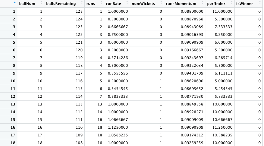
In this post, I compute each batsman’s or bowler’s Win Probability Contribution (WPC) in a T20 match. This metric captures by how much the player (batsman or bowler) changed/impacted the Win Probability of the T20 match. For this computation I use my machine learning models, I had created earlier, which predicts the ball-by-ball win probability as the T20 match progresses through the 2 innings of the match.
In the picture snippet below, you can see how the win probability changes ball-by-ball for each batsman for a T20 match between CSK vs LSG- 31 Mar 2022
In my previous posts I had created several Machine Learning models. In order to compute the player’s Win Probability contribution in this post, I have used the following ML models
The batsman’s or bowler’s win probability contribution changes ball-by=ball. The player’s contribution is calculated as the difference in win probability when the batsman faces the 1st ball in his innings and the last ball either when is out or the innings comes to an end. If the difference is +ve the the player has had a positive impact, and likewise for negative contribution. Similarly, for a bowler, it is the win probability when he/she comes into bowl till, the last delivery he/she bowls
Note: The Win Probability Contribution does not have any relation to the how much runs or at what strike rate the batsman scored the runs. Rather the model computes different win probability for each player, based on his/her embedding, the ball in the innings and six other feature vectors like runs, run rate, runsMomentum etc. These values change for every ball as seen in the table above. Also, this is not continuous. The 2 ML models determine the Win Probability for a specific player, ball and the context in the match.
This metric is similar to Win Probability Added (WPA) used in Sabermetrics for baseball. Here is the definition of WPA from Fangraphs “Win Probability Added (WPA) captures the change in Win Expectancy from one plate appearance to the next and credits or debits the player based on how much their action increased their team’s odds of winning.” This article in Fangraphs explains in detail how this computation is done.
In this post I have added 4 new function to my R package yorkr.
batsmanWinProbLR – batsman’s win probability contribution based on glmnet (Logistic Regression)
bowlerWinProbLR – bowler’s win probability contribution based on glmnet (Logistic Regression)
batsmanWinProbDL – batsman’s win probability contribution based on Deep Learning Model
bowlerWinProbDL – bowlerWinProbLR – bowler’s win probability contribution based on Deep Learning
Hence there are 4 additional features in GooglyPlusPlus based on the above 4 functions. In addition I have also updated
-winProbLR (overLap) function to include the names of batsman when they come to bat and when they get out or the innings comes to an end, based on Logistic Regression
-winProbDL(overLap) function to include the names of batsman when they come to bat and when they get out based on Deep Learning
Hence there are 6 new features in this version of GooglyPlusPlus.
Note: All these new 6 features are available for all 9 formats of T20 in GooglyPlusPlus namely
a) IPL b) BBL c) NTB d) PSL e) Intl, T20 (men) f) Intl. T20 (women) g) WBB h) CSL i) SSM
Check out the latest version of GooglyPlusPlus at gpp2023-2
Note: The data for GooglyPlusPlus comes from Cricsheet and the Shiny app is based on my R package yorkr
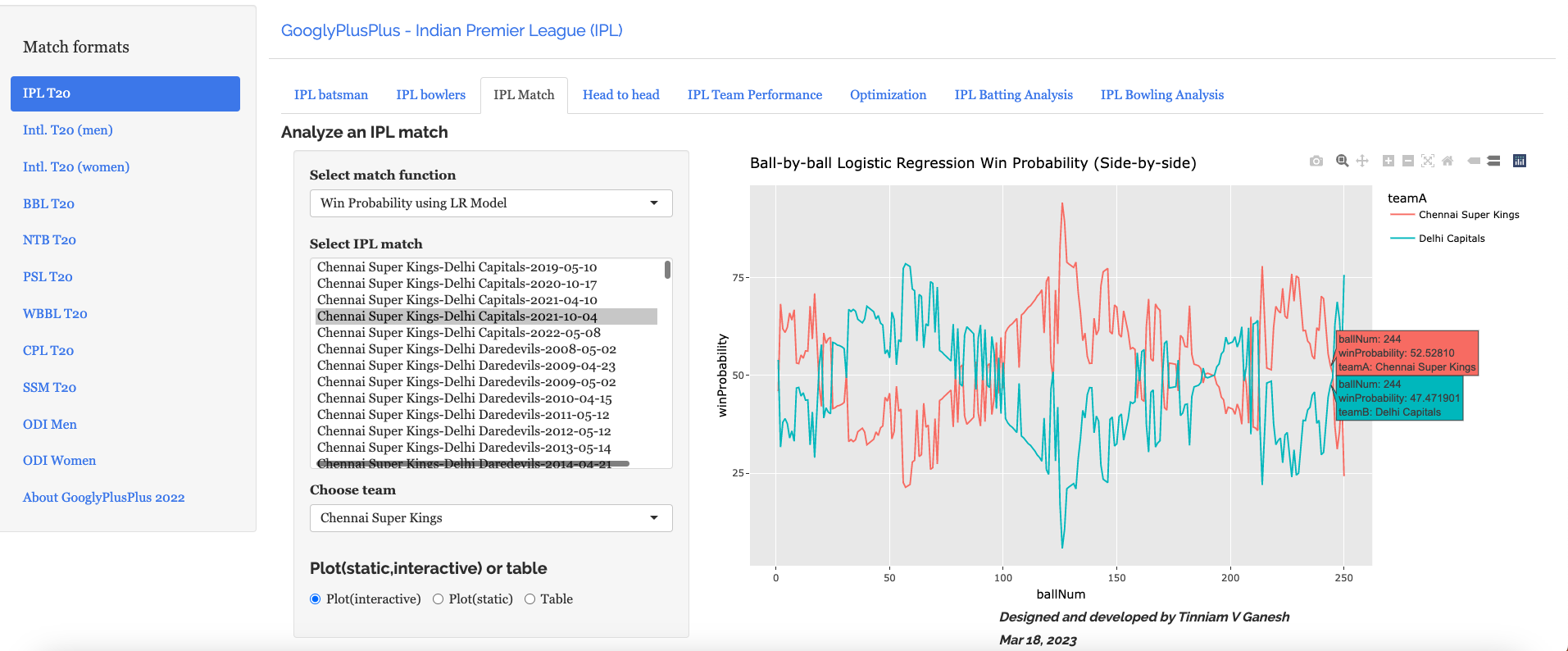
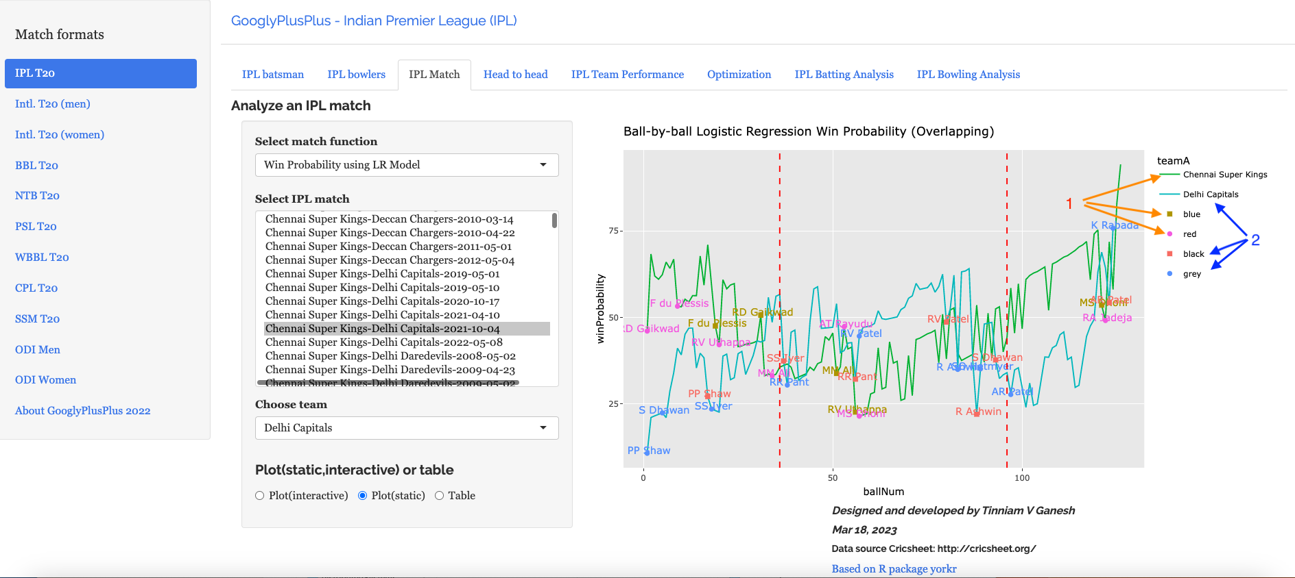
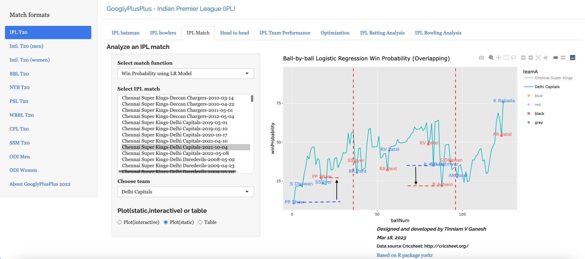
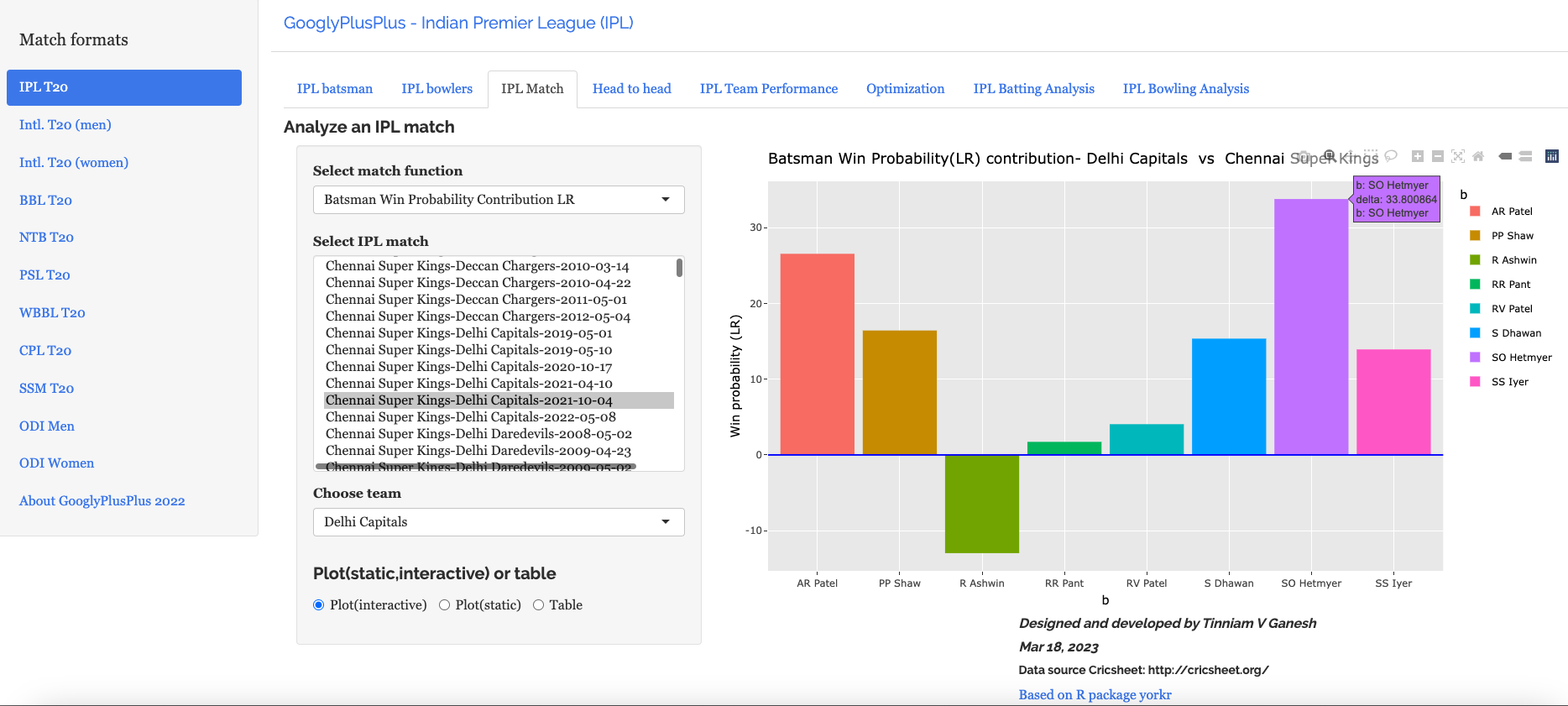
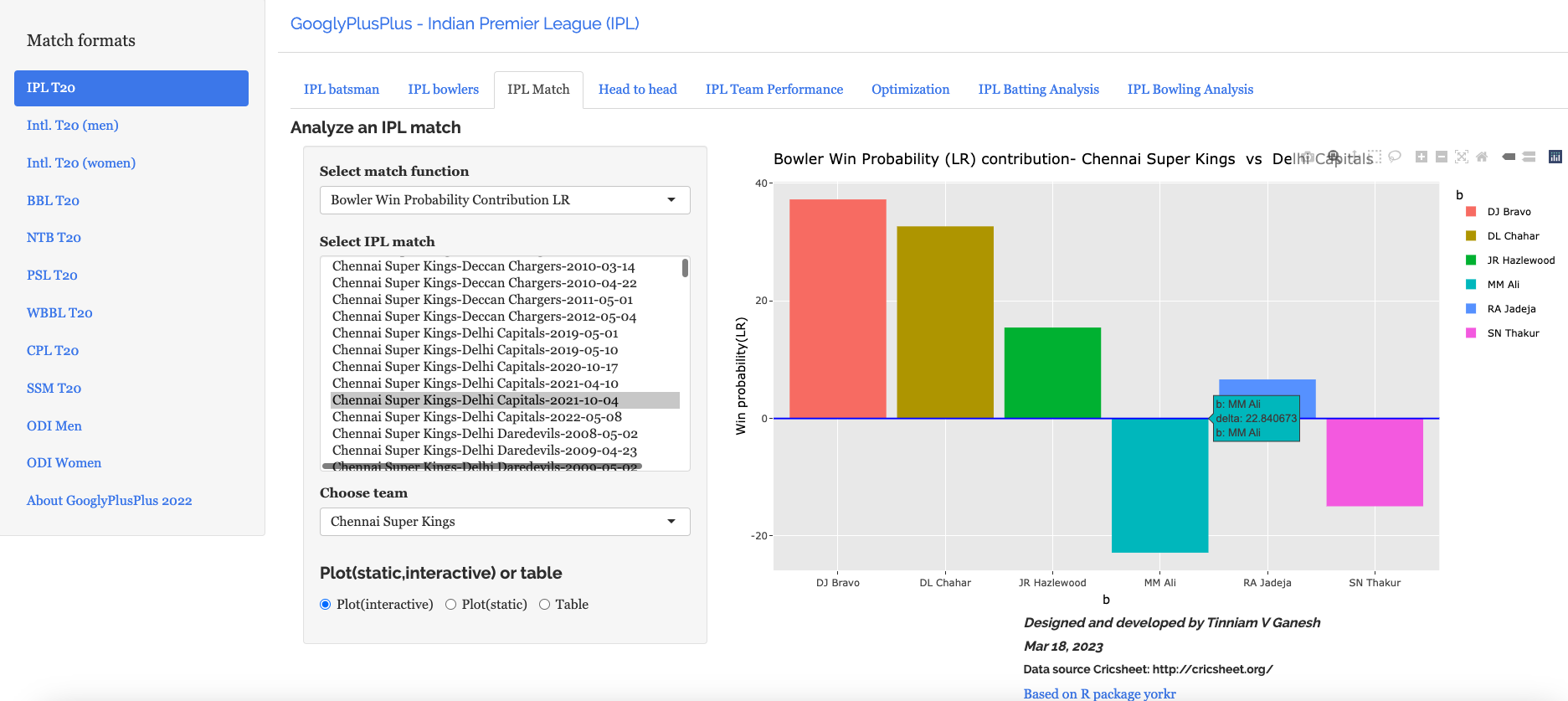
A) Chennai SuperKings vs Delhi Capitals – 04 Oct 2021
To understand Win Probability Contribution better let us look at Chennai Super Kings vs Delhi Capitals match on 04 Oct 2021
This was closely fought match with fortunes swinging wildly. If we take a look at the Worm wicket chart of this match
a) Worm Wicket chart – CSK vs DC – 04 Oct 2021
Delhi Capitals finally win the match
b) Win Probability Logistic Regression (side-by-side) – CSK vs DC – 4 Oct 2021
Plotting how win probability changes over the course of the match using Logistic Regression Model
In this match Delhi Capitals won. The batting scorecard of Delhi Capitals
c) Batting Scorecard of Delhi Capitals – CSK vs DC – 4 Oct 2021
d) Win Probability Logistic Regression (Overlapping) – CSK vs DC – 4 Oct 2021
The Win Probability LR (overlapping) shows the probability function of both teams superimposed over one another. The plot includes when a batsman came into to play and when he got out. This is for both teams. This looks a little noisy, but there is a way to selectively display the change in Win Probability for each team. This can be done , by clicking the 3 arrows (orange or blue) from top to bottom. First double-click the team CSK or DC, then click the next 2 items (blue,red or black,grey) Sorry the legends don’t match the colors! 😦
Below we can see how the win probability changed for Delhi Capitals during their innings, as batsmen came into to play. See below
e)Batsman Win Probability contribution:DC – CSK vs DC – 4 Oct 2021
Computing the individual batsman’s Win Contribution and plotting we have. Hetmeyer has a higher Win Probability contribution than Shikhar Dhawan depsite scoring fewer runs
f) Bowler’s Win Probability contribution :CSK – CSK vs DC – 4 Oct 2021
We can also check the Win Probability of the bowlers. So for e.g the CSK bowlers and which bowlers had the most impact. Moeen Ali has the least impact in this match
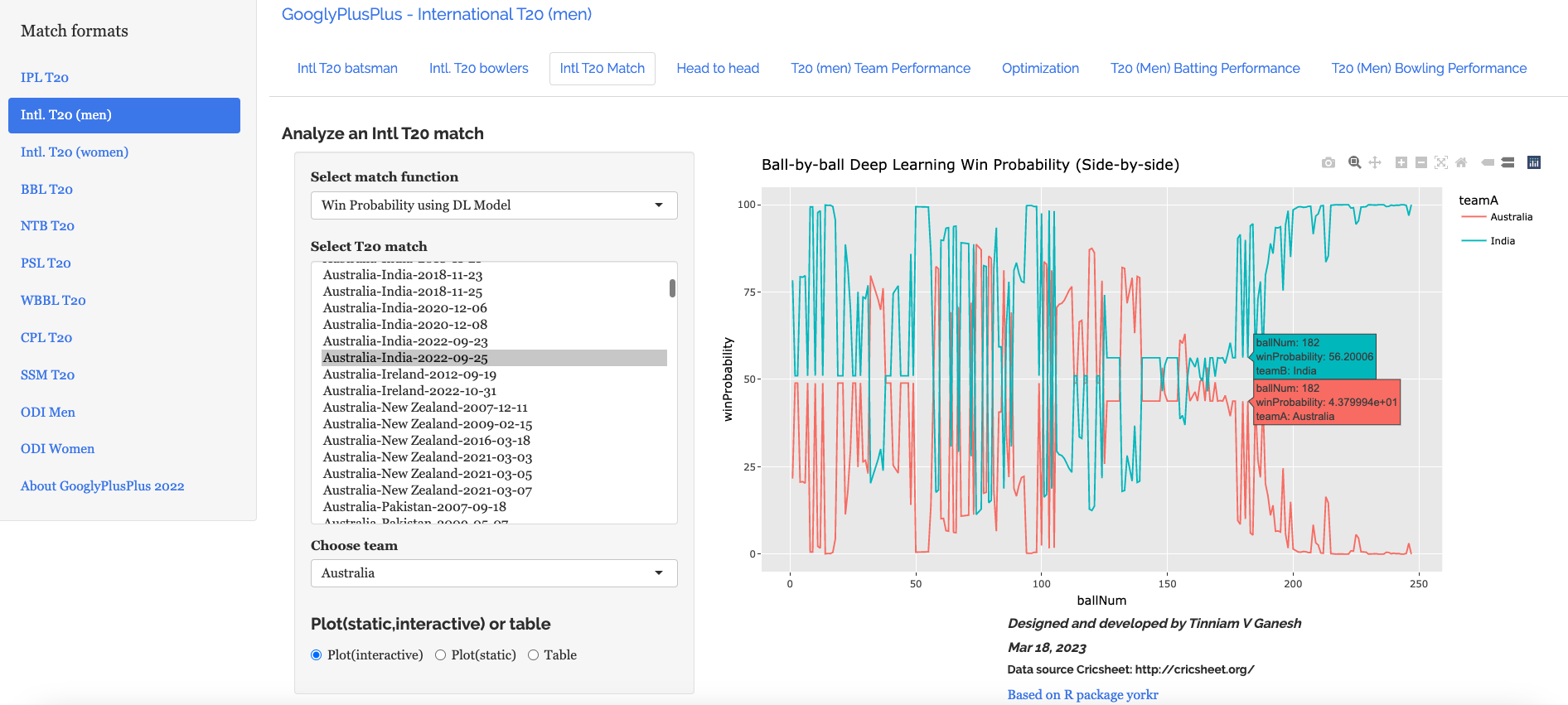
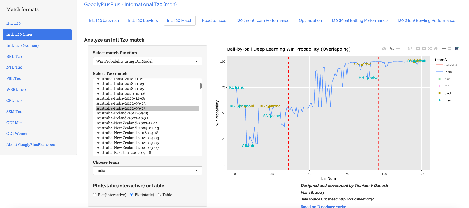
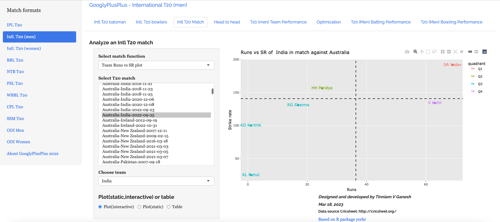
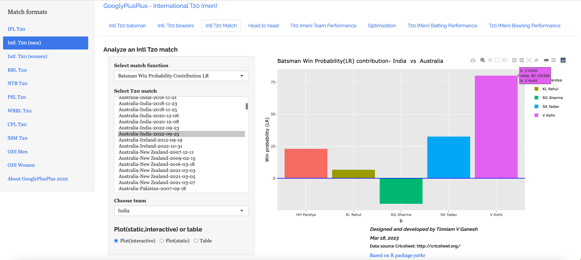
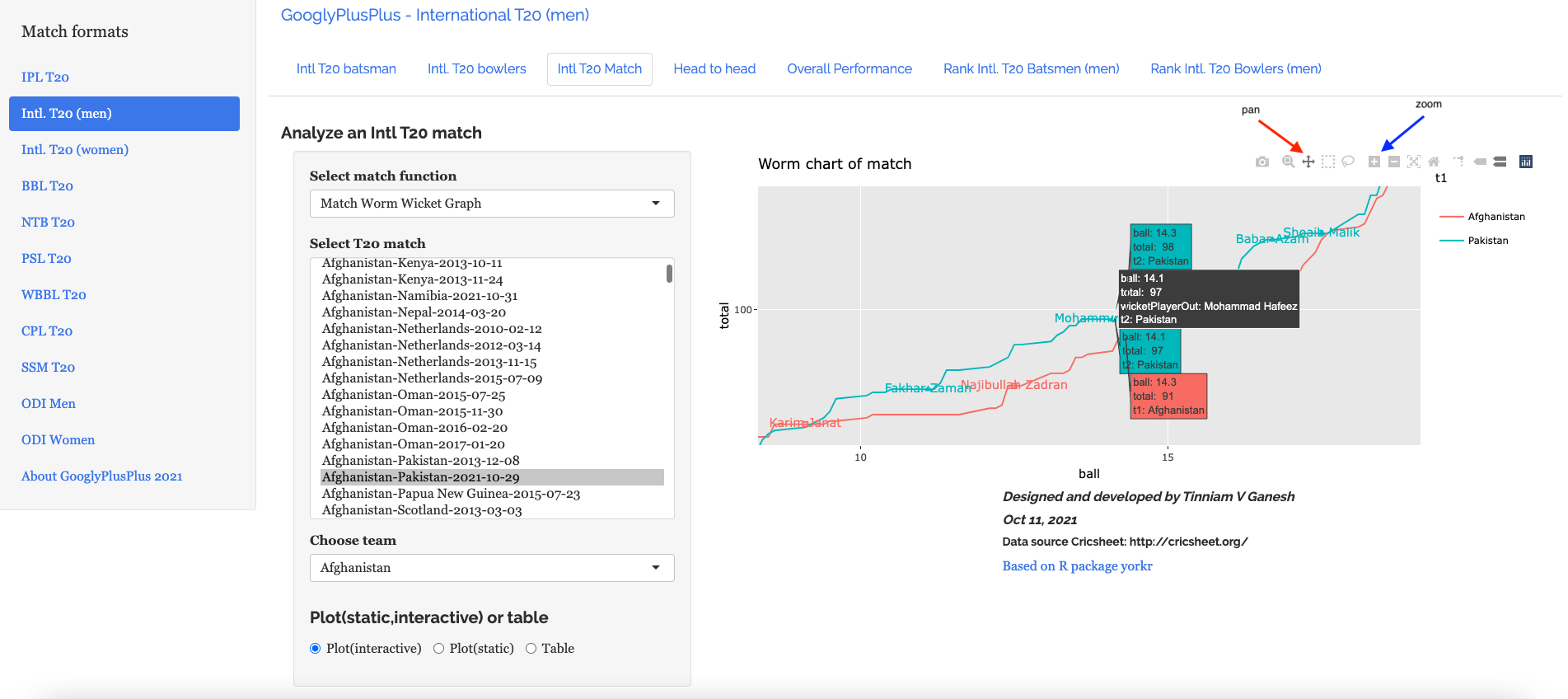
B) Intl. T20 (men) Australia vs India – 25 Sep 2022
a) Worm wicket chart – Australia vs India – 25 Sep 2022
This was another close match in which India won with the penultimate ball
b) Win Probability based on Deep Learning model (side-by-side) –Australia vs India – 25 Sep 2022
c) Win Probability based on Deep Learning model (overlapping) –Australia vs India – 25 Sep 2022
The plot below shows how the Win Probability of the teams varied across the 20 overs. The 2 Win Probability distributions are superimposed over each other
d) Batsman Win Probability Contribution : India – Australia vs India – 25 Sep 2022
Selectively choosing the India Win Probability plot by double-clicking legend ‘India’ on the right , followed by single click of black, grey legend we have
We see that Kohli, Suryakumar Yadav have good contribution to the Win Probability
e) Plotting the Runs vs Strike Rate:India – Australia vs India – 25 Sep 2022
f) Batsman’s Win Probability Contribution-Australia vs India – 25 Sep 2022
Finally plotting the Batsman’s Win Probability Contribution
Interestingly, Kohli has a greater Win Probability Contribution than SKY, though SKY scored more runs at a better strike rate. As mentioned above, the Win Probability is context dependent and also depends on past performances of the player (batsman, bowler)
Finally let us look at
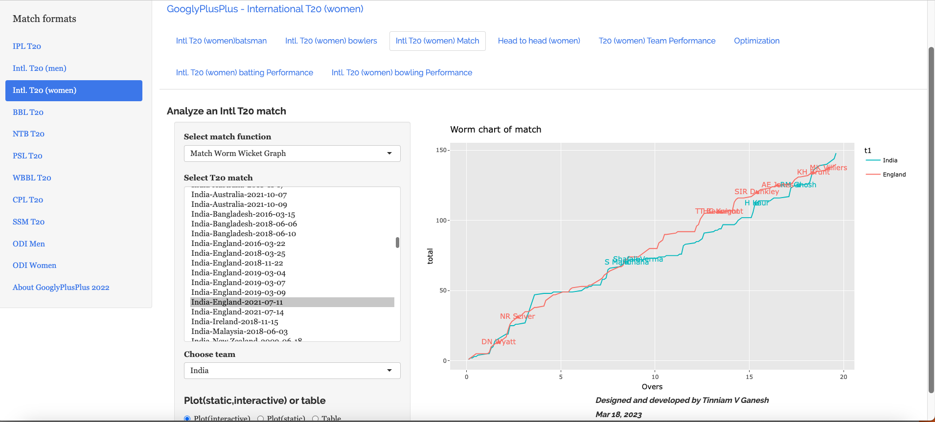
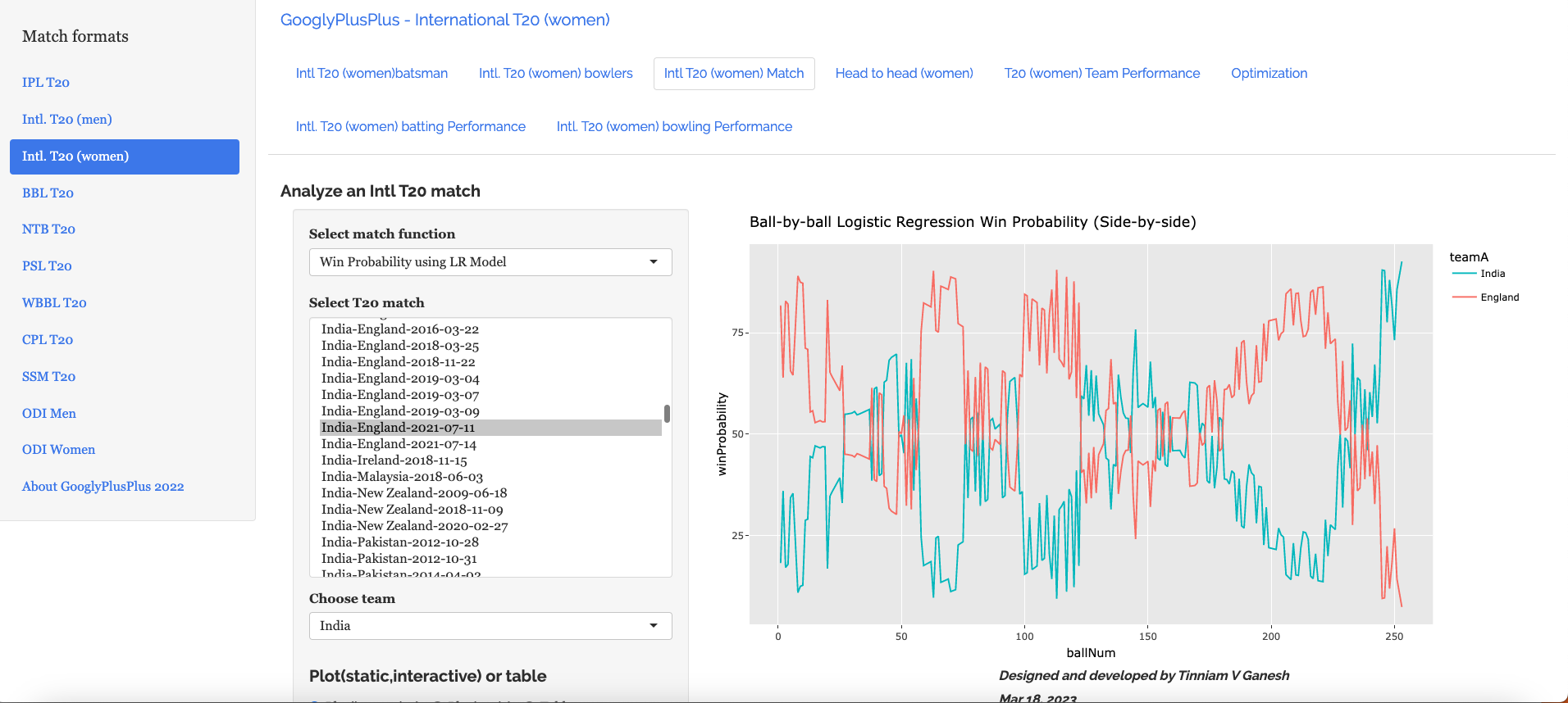
C) India vs England Intll T20 Women (11 July 2021)
a) Worm wicket chart – India vs England Intl. T20 Women (11 July 2021)
India won this T20 match by 8 runs
b) Win Probability using the Logistic Regression Model –India vs England Intl. T20 Women (11 July 2021)
c) Win Probability with the DL model –India vs England Intl. T20 Women (11 July 2021)
d) Bowler Win Probability Contribution with the LR model–India vs England Intl. T20 Women (11 July 2021)
e) Bowler Win Contribution with the DL model–India vs England Intl. T20 Women (11 July 2021)
Go ahead and try out the latest version of GooglyPlusPlus
In my previous post Computing Win Probability of T20 matches I had discussed various approaches on computing Win Probability of T20 matches. I had created ML models with glmnet and random forest using TidyModels. This was what I had achieved
glmnet : accuracy – 0.67 and sensitivity/specificity – 0.68/0.65
random forest : accuracy – 0.737 and roc_auc- 0.834
DL model with Keras in Python : accuracy – 0.73
I wanted to see if the performance of the models could be further improved. I got a suggestion from a AI/DL whizkid, who is close to me, to include embeddings for batsmen and bowlers. He felt that win percentage is influenced by which batsman faces which bowler.
So, I started to explore this idea. Embeddings can be used to convert categorical variables to a vector of continuous floating point numbers.Fortunately R’s Tidymodels, has a convenient functionality to create embeddings. By including embeddings for batsman, bowler the performance of my ML models improved vastly. Now the performance is
glmnet : accuracy – 0.728 and roc_auc – 0.81
random forest : accuracy – 0.927 and roc_auc – 0.98
mlp-dnn :accuracy – 0.762 and roc_auc – 0.854
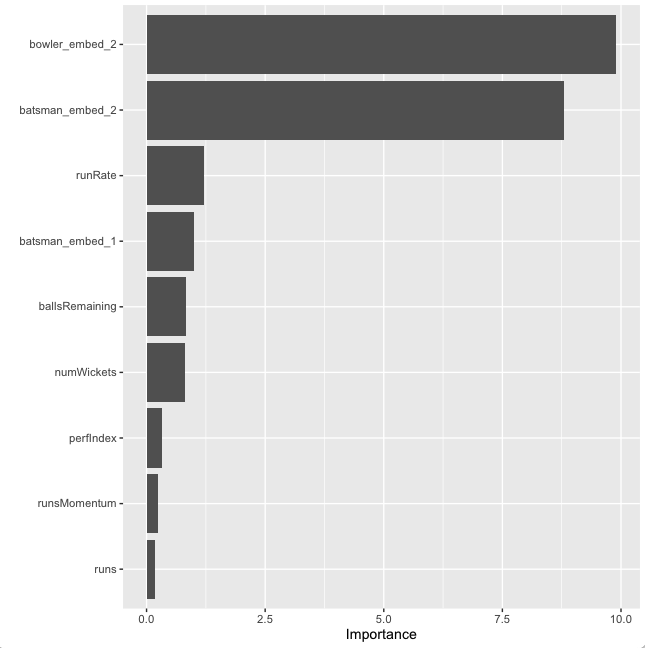
As can be seem there is almost a 20% increase in accuracy with random forests with embeddings over the model without embeddings. Moreover, the feature importance which is plotted below shows that the bowler and batsman embeddings have a significant influence on the Win Probability
Note: The data for this analysis is taken from Cricsheet and has been processed with my R package yorkr.
A. Win Probability using GLM with penalty and player embeddings
Here Generalised Linear Model (GLMNET) for Logistic Regression is used. In the GLMNET the regularisation path is computed for the lasso or elastic net penalty at a grid of values for the regularisation parameter lambda. glmnet is extremely fast and gave an accuracy of 0.72 for an roc_auc of 0.81 with batsman, bowler embeddings. This was good improvement over my earlier implementation with glmnet without the batsman & bowler embeddings which had a
Read the data
a) Read the data from 9 T20 leagues (BBL, CPL, IPL, NTB, PSL, SSM, T20 Men, T20 Women, WBB) and create a single data frame of ball-by-ball data. Display the data frame
b) Split to training, validation and test sets. The dataset is initially split into training and test in the ratio 80%:20%. The training data is again split into training and validation in the ratio 80:20
4) Create a Logistic Regression Workflow by adding the GLM model and the recipe
5) Create grid of elastic penalty values for regularisation
6) Train all 30 models
7) Plot the ROC of the model against the penalty
# Use all 12 cores
cores <- parallel::detectCores()
cores
# Create a Logistic Regression model with penalty
lr_mod <-
logistic_reg(penalty = tune(), mixture = 1) %>%
set_engine("glmnet",num.threads = cores)
# Create pre-processing recipe
lr_recipe <-
recipe(isWinner ~ ., data = df_other) %>%
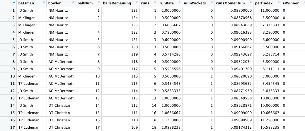
step_embed(batsman,bowler, outcome = vars(isWinner)) %>% step_normalize(ballNum,ballsRemaining,runs,runRate,numWickets,runsMomentum,perfIndex)
# Set the workflow by adding the GLM model with the recipe
lr_workflow <-
workflow() %>%
add_model(lr_mod) %>%
add_recipe(lr_recipe)
# Create a grid for the elastic net penalty
lr_reg_grid <- tibble(penalty = 10^seq(-4, -1, length.out = 30))
lr_reg_grid %>% top_n(-5)
# A tibble: 5 × 1
penalty
<dbl>
1 0.0001
2 0.000127
3 0.000161
4 0.000204
5 0.000259
lr_reg_grid %>% top_n(5) # highest penalty values
# A tibble: 5 × 1
penalty
<dbl>
1 0.0386
2 0.0489
3 0.0621
4 0.0788
5 0.1
# Train 30 penalized models
lr_res <-
lr_workflow %>%
tune_grid(val_set,
grid = lr_reg_grid,
control = control_grid(save_pred = TRUE),
metrics = metric_set(accuracy,roc_auc))
# Plot the penalty versus ROC
lr_plot <-
lr_res %>%
collect_metrics() %>%
ggplot(aes(x = penalty, y = mean)) +
geom_point() +
geom_line() +
ylab("Area under the ROC Curve") +
scale_x_log10(labels = scales::label_number())
lr_plot
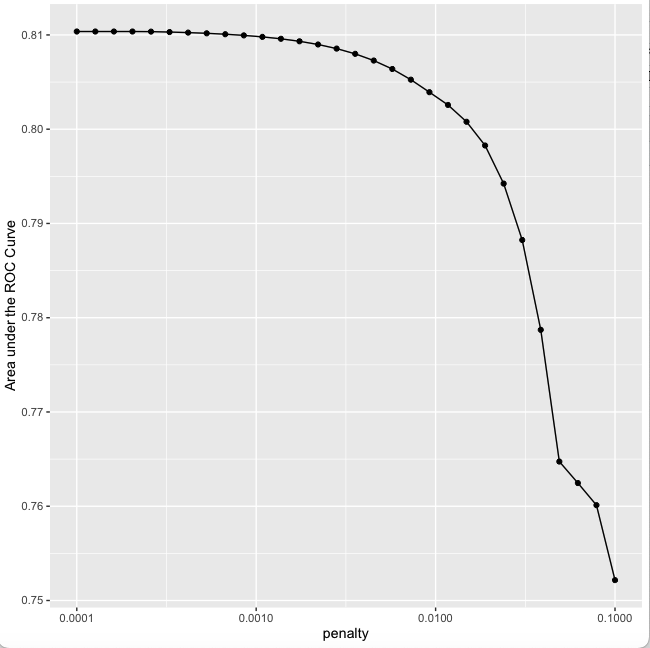
The Penalty vs ROC plot is shown below
8) Display the ROC_AUC of the top models with the penalty
9) Select the model with the best ROC_AUC and the associated penalty. It can be seen the best mean ROC_AUC is 0.81 and the associated penalty is 0.000530
top_models <-
lr_res %>%
show_best("roc_auc", n = 15) %>%
arrange(penalty)
top_models
# A tibble: 15 × 7
penalty .metric .estimator mean n std_err .config
<dbl> <chr> <chr> <dbl> <int> <dbl> <chr>
1 0.0001 roc_auc binary 0.810 1 NA Preprocessor1_Model01
2 0.000127 roc_auc binary 0.810 1 NA Preprocessor1_Model02
3 0.000161 roc_auc binary 0.810 1 NA Preprocessor1_Model03
4 0.000204 roc_auc binary 0.810 1 NA Preprocessor1_Model04
5 0.000259 roc_auc binary 0.810 1 NA Preprocessor1_Model05
6 0.000329 roc_auc binary 0.810 1 NA Preprocessor1_Model06
7 0.000418 roc_auc binary 0.810 1 NA Preprocessor1_Model07
8 0.000530 roc_auc binary 0.810 1 NA Preprocessor1_Model08
9 0.000672 roc_auc binary 0.810 1 NA Preprocessor1_Model09
10 0.000853 roc_auc binary 0.810 1 NA Preprocessor1_Model10
11 0.00108 roc_auc binary 0.810 1 NA Preprocessor1_Model11
12 0.00137 roc_auc binary 0.810 1 NA Preprocessor1_Model12
13 0.00174 roc_auc binary 0.809 1 NA Preprocessor1_Model13
14 0.00221 roc_auc binary 0.809 1 NA Preprocessor1_Model14
15 0.00281 roc_auc binary 0.809 1 NA Preprocessor1_Model15
#Picking the best model and the corresponding penalty
lr_best <-
lr_res %>%
collect_metrics() %>%
arrange(penalty) %>%
slice(8)
lr_best
# A tibble: 1 × 7
penalty .metric .estimator mean n std_err .config
<dbl> <chr> <chr> <dbl> <int> <dbl> <chr>
1 0.000530 roc_auc binary 0.810 1 NA Preprocessor1_Model08
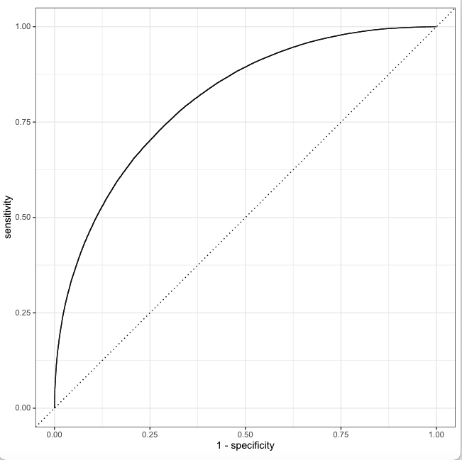
# Collect predictions and generate the AUC curve
lr_auc <-
lr_res %>%
collect_predictions(parameters = lr_best) %>%
roc_curve(isWinner, .pred_0) %>%
mutate(model = "Logistic Regression")
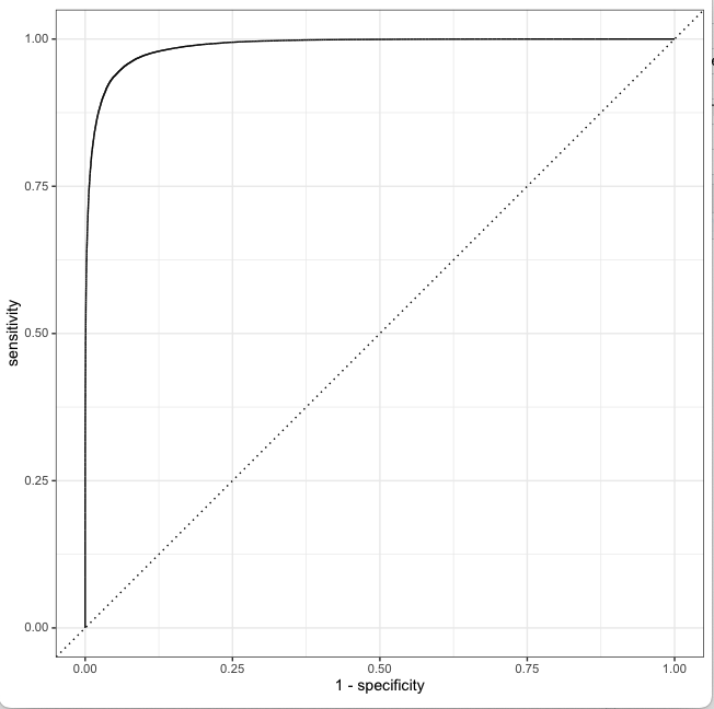
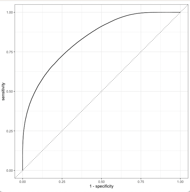
autoplot(lr_auc)
7) Plot the Area under the Curve (AUC).
10) Build the final model with the best LR parameters value as found in lr_best
a) The best performance was for a penalty of 0.000530
b) The accuracy achieved is 0.72. Clearly using the embeddings for batsman, bowlers improves on the performance of the GLM model without the embeddings. The accuracy achieved was 0.72 whereas previously it was 0.67 see (Computing Win Probability of T20 Matches)
c) Create a fit with the best parameters
d) The accuracy is 72.8% and the ROC_AUC is 0.813
# Create a model with the penalty for best ROC_AUC
last_lr_mod <-
  logistic_reg(penalty = 0.000530, mixture = 1) %>%
  set_engine("glmnet",num.threads = cores,importance = "impurity")

#Update the workflow with this model
last_lr_workflow <-
  lr_workflow %>%
  update_model(last_lr_mod)

#Create a fit
set.seed(345)
last_lr_fit <-
  last_lr_workflow %>%
  last_fit(splits)

#Generate accuracy, roc_auc
last_lr_fit %>%
  collect_metrics()
# A tibble: 2 × 4
  .metric  .estimator .estimate .config

<chr>    <chr>          <dbl> <chr>
1 accuracy binary         0.728 Preprocessor1_Model1

2 roc_auc  binary         0.813 Preprocessor1_Model1
11) Plot the feature importance
It can be seen that bowler and batsman embeddings are the most significant for the prediction followed by runRate.
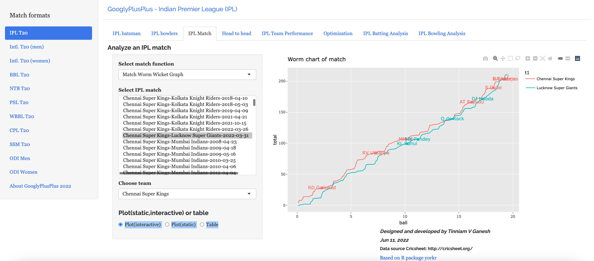
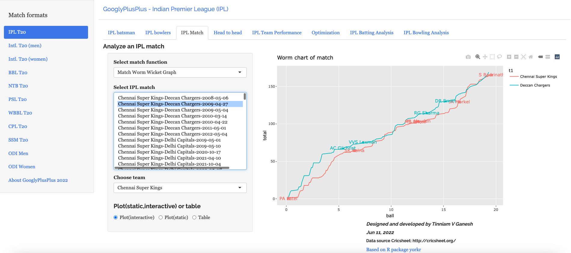
Chennai Super Kings-Lucknow Super Giants-2022-03-31
16a) The corresponding Worm-wicket graph for this match is as below
Chennai Super Kings-Lucknow Super Giants-2022-03-31
B) Win Probability using Random Forest with player embeddings
In the 2nd approach I use Random Forest with batsman and bowler embeddings. The performance of the model with embeddings is quantum jump from the earlier performance without embeddings. However, the random forest is also computationally intensive.
1) Read the data
a) Read the data from 9 T20 leagues (BBL, CPL, IPL, NTB, PSL, SSM, T20 Men, T20 Women, WBB) and create a single data frame of ball-by-ball data. Display the data frame
2) Create training.validation and test sets
b) Split to training, validation and test sets. The dataset is initially split into training and test in the ratio 80%:20%. The training data is again split into training and validation in the ratio 80:20
library(dplyr)
library(caret)
library(e1071)
library(ggplot2)
library(tidymodels)
library(tidymodels)
library(embed)

# Helper packages
library(readr)       # for importing data
library(vip)
library(ranger)

# Read all the 9 T20 leagues
df1=read.csv("output3/matchesBBL3.csv")
df2=read.csv("output3/matchesCPL3.csv")
df3=read.csv("output3/matchesIPL3.csv")
df4=read.csv("output3/matchesNTB3.csv")
df5=read.csv("output3/matchesPSL3.csv")
df6=read.csv("output3/matchesSSM3.csv")
df7=read.csv("output3/matchesT20M3.csv")
df8=read.csv("output3/matchesT20W3.csv")
df9=read.csv("output3/matchesWBB3.csv")

# Bind into a single dataframe
df=rbind(df1,df2,df3,df4,df5,df6,df7,df8,df9)

set.seed(123)
df$isWinner = as.factor(df$isWinner)

#Split data into training, validation and test sets
splits      <- initial_split(df,prop = 0.80)
df_other <- training(splits)
df_test  <- testing(splits)
set.seed(234)
val_set <- validation_split(df_other, prop = 0.80)
val_set
2) Create a Random Forest model tuning for number of predictor nodes at each decision node (mtry) and minimum number of predictor nodes (min_n)
3) Use the ranger engine and set up for classification
4) Set up the recipe and include batsman and bowler embeddings
5) Create a workflow and add the recipe and the random forest model with the tuning parameters
# Use all 12 cores parallely
cores <- parallel::detectCores()
cores
[1] 12

# Create the random forest model with mtry and min as tuning parameters
rf_mod <-
  rand_forest(mtry = tune(), min_n = tune(), trees = 1000) %>%
  set_engine("ranger", num.threads = cores) %>%
  set_mode("classification")

# Setup the recipe with batsman and bowler embeddings
rf_recipe <-
  recipe(isWinner ~ ., data = df_other) %>%
  step_embed(batsman,bowler, outcome = vars(isWinner))

# Create the random forest workflow
rf_workflow <-
  workflow() %>%
  add_model(rf_mod) %>%
  add_recipe(rf_recipe)

rf_mod
# show what will be tuned
extract_parameter_set_dials(rf_mod)

set.seed(345)
# specify which values meant to tune

# Build the model
rf_res <-
  rf_workflow %>%
  tune_grid(val_set,
            grid = 10,
            control = control_grid(save_pred = TRUE),
            metrics = metric_set(accuracy,roc_auc))

# Pick the best  roc_auc and the associated tuning parameters
rf_res %>%
  show_best(metric = "roc_auc")
# A tibble: 5 × 8
   mtry min_n .metric .estimator  mean     n std_err .config
  <int> <int> <chr>   <chr>      <dbl> <int>   <dbl> <chr>
1     4     4 roc_auc binary     0.980     1      NA Preprocessor1_Model08
2     9     8 roc_auc binary     0.979     1      NA Preprocessor1_Model03

3     8    16 roc_auc binary     0.974     1      NA Preprocessor1_Model10
4     7    22 roc_auc binary     0.969     1      NA Preprocessor1_Model09

5     5    19 roc_auc binary     0.969     1      NA Preprocessor1_Model06

rf_res %>%
  show_best(metric = "accuracy")
# A tibble: 5 × 8

mtry min_n .metric  .estimator  mean     n std_err .config
  <int> <int> <chr>    <chr>      <dbl> <int>   <dbl> <chr>
1  4     4 accuracy binary    0.927     1      NA Preprocessor1_Model08

2  9     8 accuracy binary    0.926     1      NA Preprocessor1_Model03
3  8    16 accuracy binary    0.915     1      NA Preprocessor1_Model10
4  7    22 accuracy binary    0.906     1      NA Preprocessor1_Model09

5  5    19 accuracy binary    0.904     1      NA Preprocessor1_Model0
6) Select all models with the best roc_auc. It can be seen that the best roc_auc is 0.980 for mtry=4 and min_n=4
7) Get the model with the highest accuracy. The highest accuracy achieved is 0.927 or 92.7. This accuracy is also for mtry=4 and min_n=4
# Pick the best  roc_auc and the associated tuning parameters
rf_res %>%
  show_best(metric = "roc_auc")
# A tibble: 5 × 8
   mtry min_n .metric .estimator  mean     n std_err .config
  <int> <int> <chr>   <chr>      <dbl> <int>   <dbl> <chr>
1     4     4 roc_auc binary     0.980     1      NA Preprocessor1_Model08
2     9     8 roc_auc binary     0.979     1      NA Preprocessor1_Model03

3     8    16 roc_auc binary     0.974     1      NA Preprocessor1_Model10
4     7    22 roc_auc binary     0.969     1      NA Preprocessor1_Model09

5     5    19 roc_auc binary     0.969     1      NA Preprocessor1_Model06

# Display the accuracy of the models in descending order and the parameters
rf_res %>%
  show_best(metric = "accuracy")
# A tibble: 5 × 8

mtry min_n .metric  .estimator  mean     n std_err .config
  <int> <int> <chr>    <chr>      <dbl> <int>   <dbl> <chr>
1  4     4 accuracy binary    0.927     1      NA Preprocessor1_Model08

2  9     8 accuracy binary    0.926     1      NA Preprocessor1_Model03
3  8    16 accuracy binary    0.915     1      NA Preprocessor1_Model10
4  7    22 accuracy binary    0.906     1      NA Preprocessor1_Model09

5  5    19 accuracy binary    0.904     1      NA Preprocessor1_Model0
8) Select the model with the best parameters for accuracy mtry=4 and min_n=4. For this the accuracy is 0.927. For this configuration the roc_auc is also the best at 0.980
9) Plot the Area Under the Curve (AUC). It can be seen that this model performs really well and it hugs the top left.
# Pick the best model
rf_best <-
  rf_res %>%
  select_best(metric = "accuracy")

# The best model has mtry=4 and min=4
rf_best
     mtry min_n .config
  <int> <int> <chr>
1     4     4      Preprocessor1_Model08

#Plot AUC
rf_auc <-
  rf_res %>%
  collect_predictions(parameters = rf_best) %>%
  roc_curve(isWinner, .pred_0) %>%
  mutate(model = "Random Forest")

autoplot(rf_auc)
10) Create the final model with the best parameters
11) Execute the final fit
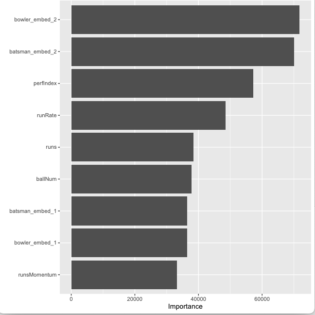
12) Plot feature importance, The bowler and batsman embedding followed by perfIndex and runRate are features that contribute the most to the Win Probability
16) Computing Win Probability with Random Forest Model for match
Pakistan-India-2022-10-23
17) Worm -wicket graph of match
Pakistan-India-2022-10-23
C) Win Probability using MLP – Deep Neural Network (DNN) with player embeddings
In this approach the MLP package of Tidymodels was used. Multi-layer perceptron (MLP) with Deep Neural Network (DNN) was used to compute the Win Probability using player embeddings. An accuracy of 0.76 was obtained
1) Read the data
a) Read the data from 9 T20 leagues (BBL, CPL, IPL, NTB, PSL, SSM, T20 Men, T20 Women, WBB) and create a single data frame of ball-by-ball data. Display the data frame
2) Create training.validation and test sets
b) Split to training, validation and test sets. The dataset is initially split into training and test in the ratio 80%:20%. The training data is again split into training and validation in the ratio 80:20
Of the 3 ML models, glmnet, random forest and Multi-layer Perceptron DNN, random forest had the best performance
Random Forest ML model with batsman, bowler embeddings was able to achieve an accuracy of 92.4% and a ROC_AUC of 0.98 with very low false positives, negatives. This was a quantum jump from my earlier random forest model without embeddings which had an accuracy of 73.7% and an ROC_AUC of 0.834
The glmnet and NN models are fairly light weight. Random Forest is computationally very intensive.
I am late to the ‘Win probability’ computation for T20 matches, but managed to jump on to this bus with this post. Win Probability analysis and computation have been around for some time and are used in baseball, NFL, soccer hockey and others. On T20 cricket, the following posts from White Ball Analytics & Sports Data Science were good pointers to the general approach. The data for the Win Probability computation is taken from Cricsheet.
My initial Machine Learning models could not do better than 62% accuracy. I created a data set of ~830 IPL matches which roughly came to about 280,000 rows of ball-by-ball match data but I could not move beyond 62%. Addition of T20 men moved the needle to 64% accuracy. I spent time tuning Deep Learning networks using Tensorflow and Keras. Finally, I added T20 data from 9 T20 leagues – IPL, T20 men, T20 women, BBL, CPL, NTB, PSL, WBB, SSM. I had one large data set of 1.2 million rows of ball by ball data. The data frame looks like
I created a data frame for each match from ball Num 1 to ballNum ~240 for the 1st and 2nd innings of the match. My initial set of features were ballNum, runs, runRate, numWickets. The target variable isWinner= {0,1} depending on whether the team has won or lost the match.
The features
ballNum – ball number for 1 ~ 240+ in data frame. 1 – 120+ for 1st innings and 120+ – 240+ in 2nd innings including noballs, wides etc.
runs = cumulative runs scored at the ball count
runRate = cumulative runs scored/ ballNum (for 1st innings) and runs= required runs/ball Num for 2nd innings
numWickets = wickets lost
The target variable isWinner can take values {0,1} depending whether the team won or lost
With this initial dataframe, even though I had close to 1.2 million rows of ball by ball data of T20 matches my best performance with vanilla Logistic regression & SVM in Python was about 64% accuracy.
# Read all the data from 9 T20 leagues
# BBL,CPL, IPL, NTB, PSL, SSM, T20 Men, T20 Women, WBB
df1=pd.read_csv('matchesT20M.csv')
df2=pd.read_csv('matchesIPL.csv')
df3=pd.read_csv('matchesBBL.csv')
df4=pd.read_csv('matchesCPL.csv')
df5=pd.read_csv('matchesNTB.csv')
df6=pd.read_csv('matchesPSL.csv')
df7=pd.read_csv('matchesSSM.csv')
df8=pd.read_csv('matchesT20W.csv')
df9=pd.read_csv('matchesWBB.csv')

# Create one large dataframe
df10=pd.concat([df1,df2,df3,df4,df5,df6,df7,df8,df9])
print("Shape of dataframe=",df10.shape)
print("#####################################")
stats=check_values(df10)
print("#####################################")
model_fit(df10)
#norm_model_fit(df,stats)
svm_model_fit(df10)

Shape of dataframe= (1206901, 6)
#####################################
Null values: False
It contains 0 infinite values

Accuracy of Logistic regression classifier on training set: 0.63
Accuracy of Logistic regression classifier on test set: 0.64
Accuracy: 0.64
Precision: 0.62
Recall: 0.65
F1: 0.64


Accuracy of Linear SVC classifier on training set: 0.52
Accuracy of Linear SVC classifier on test set: 0.52
With Tensorflow/Keras the performance was about 67%. I tried several things
Normalisation
Tried different learning rates
Different optimisers – SGD, RMSProp, Adam
Changed depth and width of Neural Network
However I did not get much improvement. Finally I decided to do some Feature engineering. I added 2 new features
a) Runs Momentum : This feature is based on the fact that more the wickets in hand, the more freely the batsmen can make risky strokes, hence increasing the momentum of the runs, This is calculated as
runsMomentum = (11 – numWickets)/balls remaining
b) Performance Index: This feature is the product of the run rate x wickets in hand. In other words, if the strike rate is good and fewer wickets lost at the point in the match, then the performance index is higher at that point in the match will be higher
The final set of features chosen were as below
I had also included the balls Remaining in the innings. Now with this set of features I decided to execute Tensorflow/Keras and do a GridSearch with different learning rates, optimisers. After a couple of hours of computation I got an accuracy of 0.73. I needed to be able to read the ML model in R which required installation of Tensorflow, reticulate and Keras in RStudio and I had several issues. Since I hit a roadblock I moved to regular R models
I performed WIn Probability computation in the following ways
A) Win Probability with Vanilla Logistic Regression (R)
With vanilla Logistic Regression in R using the ‘glm’ package I got an accuracy of 0.67, sensitivity of 0.68 and specificity of 0.65 as shown below
library(dplyr)
library(caret)
library(e1071)
library(ggplot2)

# Read all the data from 9 T20 leagues
# BBL,CPL, IPL, NTB, PSL, SSM, T20 Men, T20 Women, WBB
df1=read.csv("output2/matchesBBL2.csv")
df2=read.csv("output2/matchesCPL2.csv")
df3=read.csv("output2/matchesIPL2.csv")
df4=read.csv("output2/matchesNTB2.csv")
df5=read.csv("output2/matchesPSL2.csv")
df6=read.csv("output2/matchesSSM2.csv")
df7=read.csv("output2/matchesT20M2.csv")
df8=read.csv("output2/matchesT20W2.csv")
df9=read.csv("output2/matchesWBB2.csv")

# Create one large dataframe
df=rbind(df1,df2,df3,df4,df5,df6,df7,df8,df9)

# Helper function to split into training/test
trainTestSplit <- function(df,trainPercent,seed1){
  ## Sample size percent
  samp_size <- floor(trainPercent/100 * nrow(df))
  ## set the seed
  set.seed(seed1)
  idx <- sample(seq_len(nrow(df)), size = samp_size)
  idx

}

train_idx <- trainTestSplit(df,trainPercent=80,seed=5)
train <- df[train_idx, ]

test <- df[-train_idx, ]
# Fit a generalized linear logistic model,
fit=glm(isWinner~.,family=binomial,data=train,control = list(maxit = 50))

a=predict(fit,newdata=train,type="response")
# Set response >0.5 as 1 and <=0.5 as 0
b=as.factor(ifelse(a>0.5,1,0))
# Compute the confusion matrix for training data

confusionMatrix(
  factor(b, levels = 0:1),
  factor(train$isWinner, levels = 0:1)
)

Confusion Matrix and Statistics

          Reference
Prediction
  0      1
         0 339938 160336
         1 154236 310217

               Accuracy : 0.6739
                 95% CI : (0.673, 0.6749)
    No Information Rate : 0.5122
    P-Value [Acc > NIR] : < 2.2e-16

                  Kappa : 0.3473

 Mcnemar's Test P-Value : < 2.2e-16

            Sensitivity : 0.6879
            Specificity : 0.6593
         Pos Pred Value : 0.6795
         Neg Pred Value : 0.6679
             Prevalence : 0.5122
         Detection Rate : 0.3524
   Detection Prevalence : 0.5186
      Balanced Accuracy : 0.6736

       'Positive' Class : 0

# This can be saved and loaded as
saveRDS(fit, "glm.rds")
ml_model <- readRDS("glm.rds")
Using the above ML model on Deccan Chargers vs Chennai Super on 27-04-2009 the Win Probability as the match progresses is as below
The Worm wicket graph of this match shows it was a closely fought match
B) Win Probability using Random Forests with Tidy Models – R
Initially I tried Tidy models with tuning for glmnet. The best I got was 0.67. However, I got an excellent performance using TidyModels with Random Forests. I am using Tidy Models for the first time and I have been blown away with how logically it is constructed, much like dplyr & ggplot2.
library(dplyr)
library(caret)
library(e1071)
library(ggplot2)
library(tidymodels)

# Helper packages
library(readr)       # for importing data
library(vip)
library(ranger)
# Read all the data from 9 T20 leagues
# BBL,CPL, IPL, NTB, PSL, SSM, T20 Men, T20 Women, WBB

df1=read.csv("output2/matchesBBL2.csv")
df2=read.csv("output2/matchesCPL2.csv")
df3=read.csv("output2/matchesIPL2.csv")
df4=read.csv("output2/matchesNTB2.csv")
df5=read.csv("output2/matchesPSL2.csv")
df6=read.csv("output2/matchesSSM2.csv")
df7=read.csv("output2/matchesT20M2.csv")
df8=read.csv("output2/matchesT20W2.csv")
df9=read.csv("output2/matchesWBB2.csv")

# Create one large dataframe
df=rbind(df1,df2,df3,df4,df5,df6,df7,df8,df9)

dim(df)
[1]
1205909       8

# Take a peek at the dataset
glimpse(df)
$ ballNum        <int> 1, 2, 3, 4, 5, 6, 7, 8, 9, 10, 11, 12, 13, 14, 15, 16, 17, 18, 19, 20, 21, 22, 23, 24, 25, 26, 27, 28…
$ ballsRemaining <int> 125, 124, 123, 122, 121, 120, 119, 118, 117, 116, 115, 114, 113, 112, 111, 110, 109, 108, 107, 106, 1…
$ runs           <int> 1, 1, 2, 3, 3, 3, 4, 4, 5, 5, 6, 7, 13, 14, 16, 18, 18, 18, 24, 24, 24, 26, 26, 32, 32, 33, 34, 34, 3…
$ runRate        <dbl> 1.0000000, 0.5000000, 0.6666667, 0.7500000, 0.6000000, 0.5000000, 0.5714286, 0.5000000, 0.5555556, 0.…
$ numWickets     <int> 0, 0, 0, 0, 0, 0, 0, 0, 0, 1, 1, 1, 1, 1, 1, 1, 1, 1, 1, 2, 2, 2, 2, 2, 2, 2, 2, 3, 3, 3, 3, 3, 3, 3,…
$ runsMomentum   <dbl> 0.08800000, 0.08870968, 0.08943089, 0.09016393, 0.09090909, 0.09166667, 0.09243697, 0.09322034, 0.094…
$ perfIndex      <dbl> 11.000000, 5.500000, 7.333333, 8.250000, 6.600000, 5.500000, 6.285714, 5.500000, 6.111111, 5.000000, …
$ isWinner       <int> 0, 0, 0, 0, 0, 0, 0, 0, 0, 0, 0, 0, 0, 0, 0, 0, 0, 0, 0, 0, 0, 0, 0, 0, 0, 0, 0, 0, 0, 0, 0, 0, 0, 0,…

df %>%
  count(isWinner) %>%
  mutate(prop = n/sum(n))

set.seed(123)
df$isWinner = as.factor(df$isWinner)

# Split the data into training and test set in 80%:20%
splits      <- initial_split(df,prop = 0.80)
df_other <- training(splits)
df_test  <- testing(splits)

# Create a validation set from training set in 80%:20%
set.seed(234)
val_set <- validation_split(df_other,
                            prop = 0.80)
val_set

# Setup for Random forest using Ranger for classification
# Set up cores for parallel execution
cores <- parallel::detectCores()
cores

#Set up Random Forest engine
rf_mod <-
  rand_forest(mtry = tune(), min_n = tune(), trees = 1000) %>%
  set_engine("ranger", num.threads = cores) %>%
  set_mode("classification")

rf_mod
# The Random Forest engine includes mtry which is number of predictor
# variables required at each decision  tree with min_n the minimum number # of
Random Forest Model Specification (classification)

Main Arguments:
  mtry = tune()
  trees = 1000
  min_n = tune()

Engine-Specific Arguments:
  num.threads = cores

Computational engine: ranger


# Setup the predictors and target variable
# Normalise all predictors. Random Forest don't need normalization but
# I have done it anyway
rf_recipe <-
  recipe(isWinner ~ ., data = df_other) %>%
  step_normalize(all_predictors())

# Create workflow adding the ML model and recipe
rf_workflow <-
  workflow() %>%
  add_model(rf_mod) %>%
  add_recipe(rf_recipe)

# The tune is done for 5 different values of the tuning parameters.
# Metrics include accuracy and roc_auc
rf_res <-
  rf_workflow %>%
  tune_grid(val_set,
            grid = 5,
            control = control_grid(save_pred = TRUE),
            metrics = metric_set(accuracy,roc_auc))

$ Pick the best of ROC/AUC
rf_res %>%
  show_best(metric = "roc_auc")

We can see that when mtry (number of predictors) is 5 or 7 the ROC_AUC is 0.834 which is quite good

# A tibble: 5 × 8
   mtry min_n .metric .estimator  mean     n std_err .config
  <int> <int> <chr>   <chr>      <dbl> <int>   <dbl> <chr>
1     5    26 roc_auc binary     0.834     1      NA Preprocessor1_Model5
2     7    36 roc_auc binary     0.834     1      NA Preprocessor1_Model3
3     2    17 roc_auc binary     0.833     1      NA Preprocessor1_Model4
4     1    20 roc_auc binary     0.832     1      NA Preprocessor1_Model2
5     5     6 roc_auc binary     0.825     1      NA Preprocessor1_Model1


# Select the model with highest accuracy
rf_res %>%
  show_best(metric = "accuracy")
   mtry min_n .metric  .estimator  mean     n std_err .config
  <int> <int> <chr>    <chr>      <dbl> <int>   <dbl> <chr>
1     7    36 accuracy binary     0.737     1      NA Preprocessor1_Model3
2     5    26 accuracy binary     0.736     1      NA Preprocessor1_Model5
3     1    20 accuracy binary     0.736     1      NA Preprocessor1_Model2
4     2    17 accuracy binary     0.735     1      NA Preprocessor1_Model4
5     5     6 accuracy binary     0.731     1      NA Preprocessor1_Model1

# The model with mtry (number of predictors) is 7 has the best accuracy.
# Hence the best model has mtry=7 and min_n=36

rf_best <-
  rf_res %>%
  select_best(metric = "accuracy")

# Display the best model
rf_best
# A tibble: 1 × 3
   mtry min_n .config
  <int> <int> <chr>
1     7    36 Preprocessor1_Model3


rf_res %>%
  collect_predictions()
   id         .pred_class  .row  mtry min_n .pred_0  .pred_1 isWinner .config
   <chr>      <fct>       <int> <int> <int>   <dbl>    <dbl> <fct>    <chr>
 1 validation 1               1     5     6 0.497   0.503    0        Preprocessor1_Model1
 2 validation 1               9     5     6 0.00753 0.992    1        Preprocessor1_Model1
 3 validation 0              10     5     6 0.627   0.373    0        Preprocessor1_Model1
 4 validation 0              16     5     6 0.998   0.002    0        Preprocessor1_Model1
 5 validation 1              18     5     6 0.270   0.730    1        Preprocessor1_Model1
 6 validation 0              23     5     6 0.899   0.101    0        Preprocessor1_Model1
 7 validation 1              26     5     6 0.452   0.548    1        Preprocessor1_Model1
 8 validation 0              30     5     6 0.657   0.343    1        Preprocessor1_Model1
 9 validation 0              34     5     6 0.576   0.424    0        Preprocessor1_Model1
10 validation 0              35     5     6 1.00    0.000167 0        Preprocessor1_Model1

rf_auc <-
  rf_res %>%
  collect_predictions(parameters = rf_best) %>%
  roc_curve(isWinner, .pred_0) %>%
  mutate(model = "Random Forest")

autoplot(rf_auc)
I
The Final Model
# Create the final Random Forest model with mtry=7 and min_n=36
# engine as "ranger" for classification
last_rf_mod <-
  rand_forest(mtry = 7, min_n = 36, trees = 1000) %>%
  set_engine("ranger", num.threads = cores, importance = "impurity") %>%
  set_mode("classification")


# the last workflow is updated with the final model
last_rf_workflow <-
  rf_workflow %>%
  update_model(last_rf_mod)

set.seed(345)
last_rf_fit <-
  last_rf_workflow %>%
  last_fit(splits)

# Collect metrics
last_rf_fit %>%
  collect_metrics()
  .metric  .estimator .estimate .config
  <chr>    <chr>          <dbl> <chr>
1 accuracy binary         0.739 Preprocessor1_Model1
2 roc_auc  binary         0.837 Preprocessor1_Model1

The Random Forest model gives an accuracy of 0.739 and ROC_AUC of .837 which I think is quite good. This is roughly what I got with Tensorflow/Keras

# Get the feature importance
last_rf_fit %>%
  extract_fit_parsnip() %>%
  vip(num_features = 7)
Interestingly the feature that I engineered seems to have the maximum importancce namely Performance Index which is a product of Run rate x Wicket in Hand. I would have thought numWickets would be important but in T20 match probably is is not.
 generate predictions from the test set
test_predictions <- last_rf_fit %>% collect_predictions()
> test_predictions
# A tibble: 241,182 × 7
id               .pred_0 .pred_1  .row .pred_class isWinner .config
<chr>              <dbl>   <dbl> <int> <fct>       <fct>    <chr>
  1 train/test split   0.496   0.504     1 1           0        Preprocessor1_Model1
2 train/test split   0.640   0.360    11 0           0        Preprocessor1_Model1
3 train/test split   0.596   0.404    14 0           0        Preprocessor1_Model1
4 train/test split   0.287   0.713    22 1           0        Preprocessor1_Model1
5 train/test split   0.616   0.384    28 0           0        Preprocessor1_Model1
6 train/test split   0.516   0.484    36 0           0        Preprocessor1_Model1
7 train/test split   0.754   0.246    37 0           0        Preprocessor1_Model1
8 train/test split   0.641   0.359    39 0           0        Preprocessor1_Model1
9 train/test split   0.811   0.189    40 0           0        Preprocessor1_Model1
10 train/test split   0.618   0.382    42 0           0        Preprocessor1_Model1


# generate a confusion matrix
test_predictions %>%
  conf_mat(truth = isWinner, estimate = .pred_class)

          Truth
Prediction     0     1
         0 92173 31623
         1 31320 86066

# Create the final model on the train/test data
final_model <- fit(last_rf_workflow, df_other)

# Final model
final_model
══ Workflow [trained] ════════════════════════════════════════════════════════════════════════════════════════════════════════
Preprocessor: Recipe
Model: rand_forest()

── Preprocessor ──────────────────────────────────────────────────────────────────────────────────────────────────────────────
1 Recipe Step

• step_normalize()

── Model ─────────────────────────────────────────────────────────────────────────────────────────────────────────────────────
Ranger result

Call:
 ranger::ranger(x = maybe_data_frame(x), y = y, mtry = min_cols(~7,      x), num.trees = ~1000, min.node.size = min_rows(~36, x),      num.threads = ~cores, importance = ~"impurity", verbose = FALSE,      seed = sample.int(10^5, 1), probability = TRUE)

Type:                             Probability estimation
Number of trees:                  1000
Sample size:                      964727
Number of independent variables:  7
Mtry:                             7
Target node size:                 36
Variable importance mode:         impurity
Splitrule:                        gini
OOB prediction error (Brier s.):  0.1631303
The Random Forest Model’s performance has been quite impressive and probably requires further exploration.
# Saving and loading the model
save(final_model, file = "fit.rda")
load("fit.rda")

#Predicting the Win Probability of CSK vs DD match on 12 May 2012
Comparing this with the Worm wicket graph of this match we see that DD had no chance at all
C) Win Probability with Tensorflow/Keras with Grid Search – Python
I spent a fair amount of time tuning the hyper parameters of the Keras Deep Learning Network. Finally did go for the Grid Search. Incidentally I did ask ChatGPT to suggest code snippets for GridSearch which it promptly did!!!
import pandas as pd
import numpy as np
from zipfile import ZipFile
import tensorflow as tf
from tensorflow import keras
from tensorflow.keras import layers
from tensorflow.keras import regularizers
from sklearn.model_selection import GridSearchCV

# Define the model
def create_model(optimizer='adam'):
    tf.random.set_seed(4)
    model = tf.keras.Sequential([
        keras.layers.Dense(32, activation=tf.nn.relu, input_shape=[len(train_dataset1.keys())]),
        keras.layers.Dense(16, activation=tf.nn.relu),
        keras.layers.Dense(8, activation=tf.nn.relu),
        keras.layers.Dense(1,activation=tf.nn.sigmoid)
    ])

    # Since this is binary classification use binary_crossentropy
    model.compile(loss='binary_crossentropy',
                    optimizer=optimizer,
                    metrics='accuracy')
    return(model)

    # Create a KerasClassifier object
model = keras.wrappers.scikit_learn.KerasClassifier(build_fn=create_model)

# Define the grid of hyperparameters to search over
batch_size = [1024]
epochs = [40]
learning_rate = [0.01, 0.001, 0.0001]
optimizer = ['SGD', 'RMSprop', 'Adagrad', 'Adadelta', 'Adam', 'Adamax', 'Nadam']

param_grid = dict(dict(optimizer=optimizer,batch_size=batch_size, epochs=epochs) )
# Create the grid search object
grid_search = GridSearchCV(estimator=model, param_grid=param_grid, cv=3)

# Fit the grid search object to the training data
grid_search.fit(normalized_train_data, train_labels)

# Print the best hyperparameters
print('Best hyperparameters:', grid_search.best_params_)
# summarize results
print("Best: %f using %s" % (grid_search.best_score_, grid_search.best_params_))
means = grid_search.cv_results_['mean_test_score']
stds = grid_search.cv_results_['std_test_score']
params = grid_search.cv_results_['params']
for mean, stdev, param in zip(means, stds, params):
    print("%f (%f) with: %r" % (mean, stdev, param))
The best worked out to be the optimiser ‘Nadam’ with a learning rate of 0.001
So, the Keras Deep Learning Network gives about the same performance of Random Forest in Tidy Models. But I went with R Random Forest as it was easier to save and load the model for use with my data. Also, I am not sure whether the performance of the ML model can be improved beyond a point. However, I will continue to explore.
In my last post GooglyPlusPlus gets ready for ICC Men’s T20 World Cup, I had mentioned that GooglyPlusPlus was preparing for the big event the ICC Men’s T20 World cup. Now that the T20 World cup is underway, my Shiny app in R, GooglyPlusPlus ,will be generating near real-time analytics of matches completed the previous day. Besides the app can also do historical analysis of players, teams and matches.
The whole process is automated. A cron job will execute every day, in the morning, which will automatically download the matches of the previous day from Cricsheet, unzip them, start a pipeline which will transform and process the match data into necessary folders and finally upload the newly acquired data into my Shiny app. Hence, you will be able to access all the breathless, pulsating cricketing action in timeless, interactive plots and tables which will capture all aspects of Men’s T20 matches, namely batsman, bowler performance, match analysis, team-vs-team, team-vs-all teams besides ranking of batsmen & bowlers. Since the data is cumulative, all the analytics are historical and current.
The data for GooglyPlusPlus is taken from Cricsheet
Interest in cricket, has mushroomed in recent times around the world, with the addition of new formats which started with ODI, T20, T10, 100 ball and so on. There are leagues which host these matches at different levels around the world. While GooglyPlusPlus, provides near real-time analytics of Men’s T20 World cup, we can clearly envision a big data platform which ingests matches daily from multiple cricket formats, leagues around the world generating real-time and near real-time analytics which are essential these days to selection of teams at different levels through auctions. For more discussion on this see my posts
We could imagine a Data Lake, into which are ingested data from the different cricket formats, leagues through appropriate technology connectors. Once the data is ingested, we could have data pipelines, based on Azure ADF, Apache NiFi, Apache Airflow or Amazon EMR etc., to transform, process and enhance the data, generating real-time analytics on the fly. Recent formats like T20, T10 require more urgency in strategic thinking based on scoring within limited overs, or containing batsmen from going on a rampage within the set of overs, the analytics on a fly may help the coach to modify the batting or bowling lineup at points in match. In this context see my earlier post Using Linear Programming (LP) for optimizing bowling change or batting lineup in T20 cricket
All of these are not just possible, but are likely to become reality as more and more formats, leagues and cricket data proliferate around the world.
This post, focuses on generating near-real time analytics for ICC Men’s T20 World Cup using GooglyPlusPlus. Included below, is a sampling of the analytics that you can perform for analysing the matches. In addition you can do all the analysis included in my post GooglyPlusPlus gets ready for ICC Men’s T20 World Cup
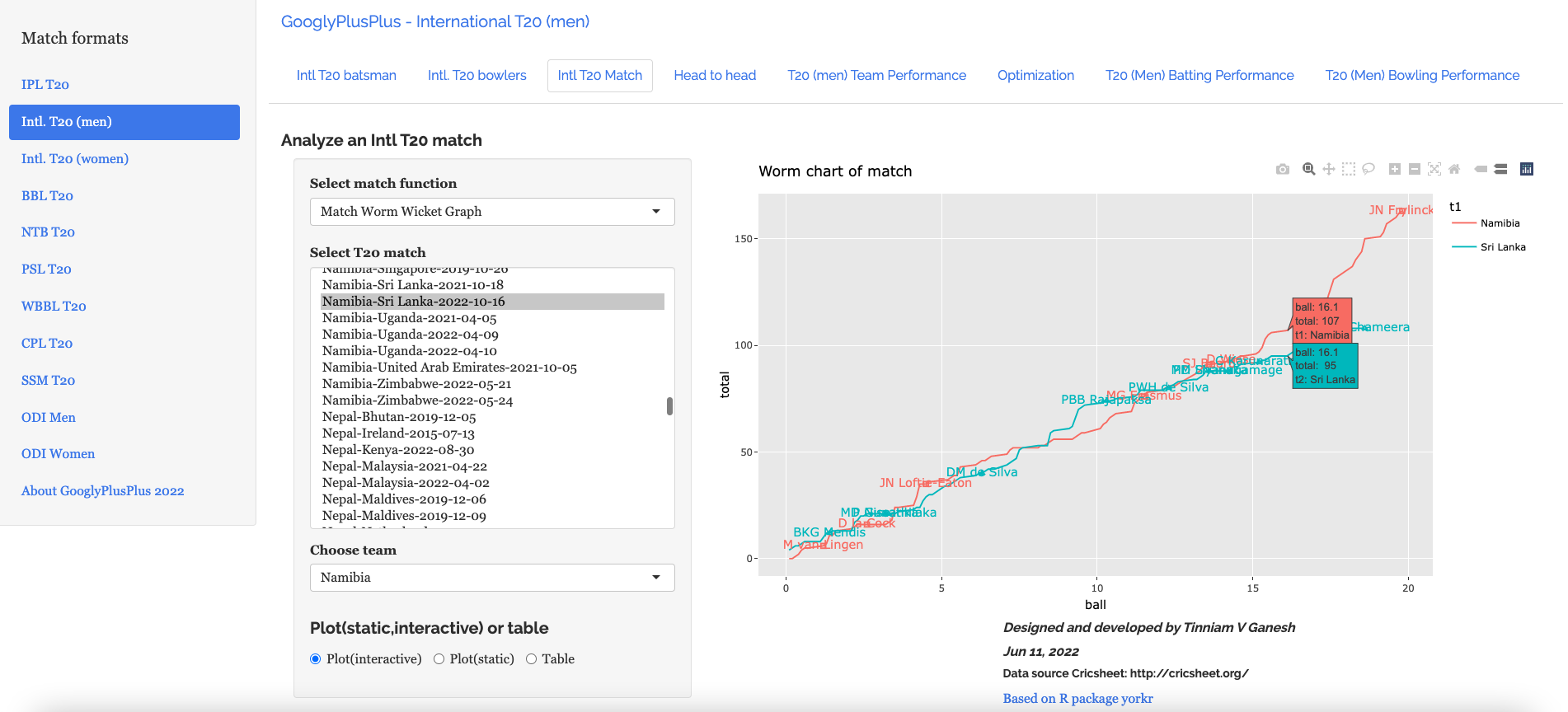
Namibia-Sri Lanka-16 Oct 2022 : Match Worm graph
The opening match between Namibia vs Sri Lanka resulted in an upset. We can see this in the match worm-wicket graph below
2. Scotland vs West Indies – 17 Oct 2022: Batsmen vs Bowlers
George Munsey was the top scorer for Scotland and was instrumental in the win against WI. His performance against West Indies bowlers is shown below. Note, the charts are interactive
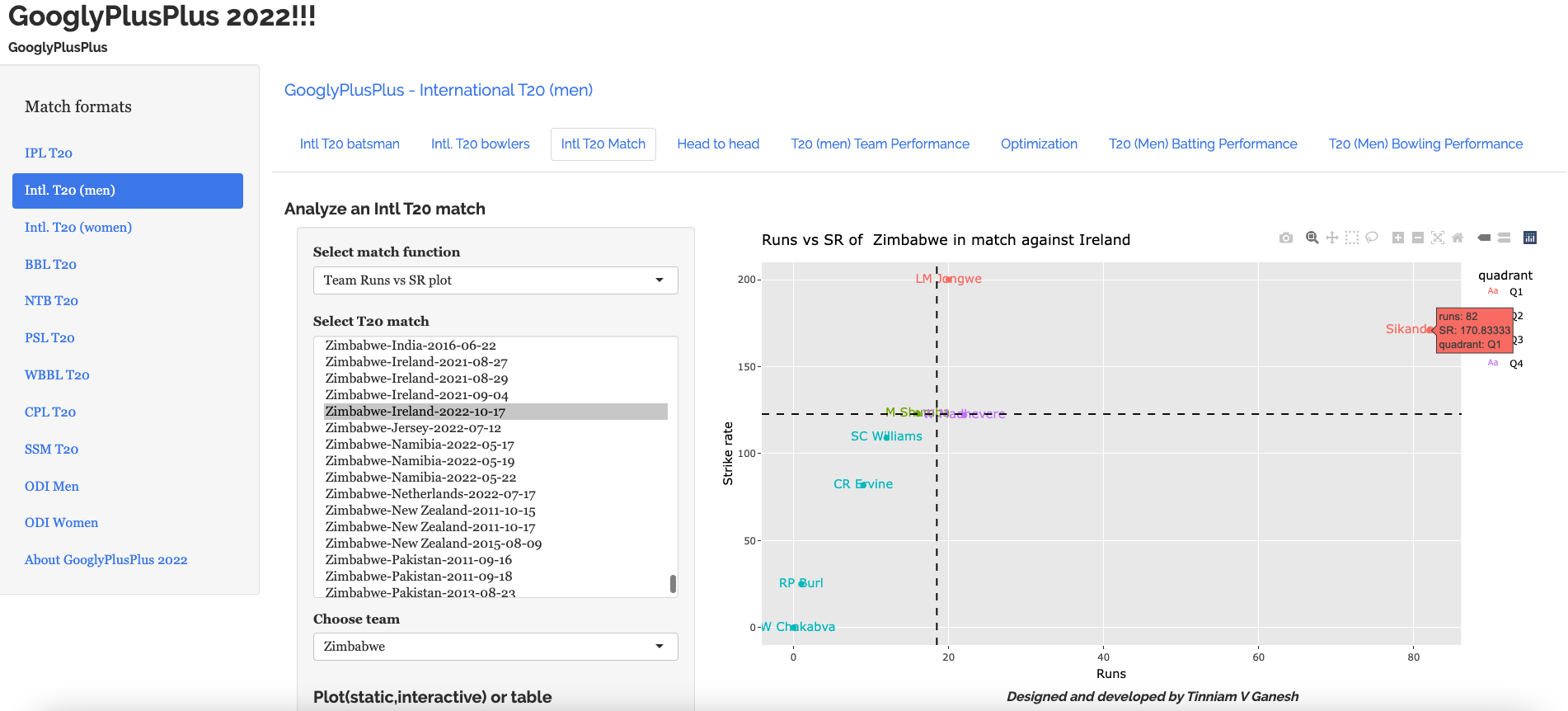
3. Zimbabwe vs Ireland – 17 Oct 2022 : Team Runs vs SR
Sikander Raza of Zimbabwe with 82 runs with the strike rate ~ 170
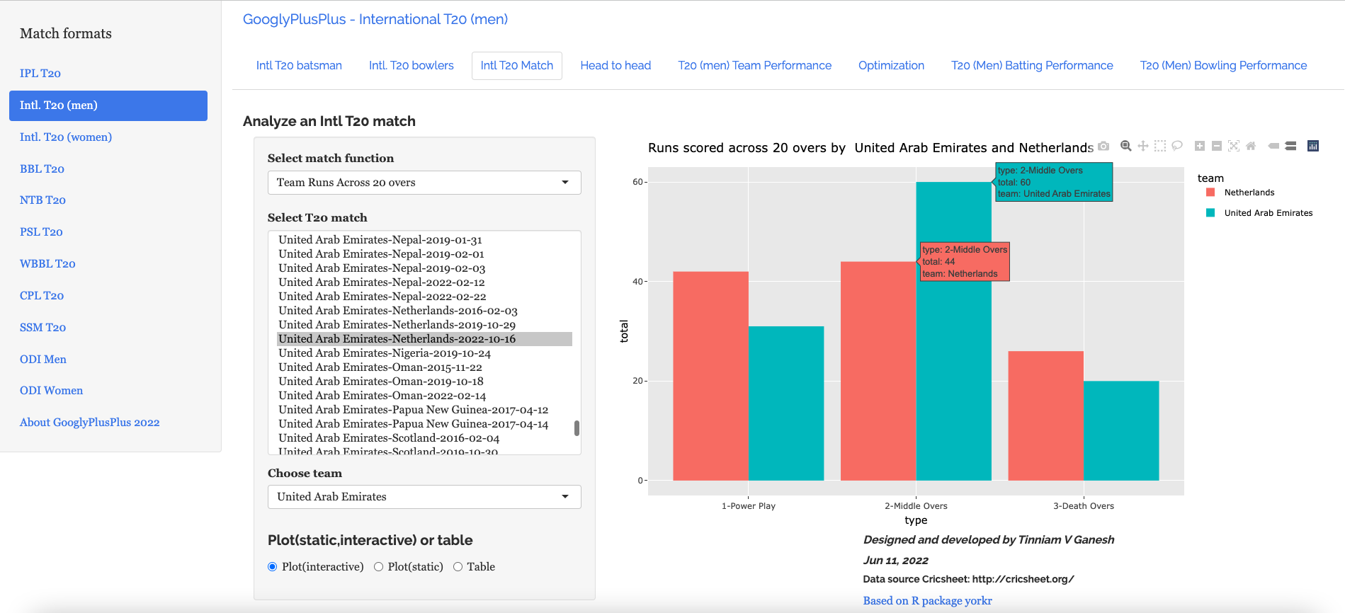
4.United Arab Emirates vs Netherlands – 16 Oct 2022: Team runs across 20 overs
UAE pipped Netherlands in the middle overs and were able to win by 1 ball and 3 wickets
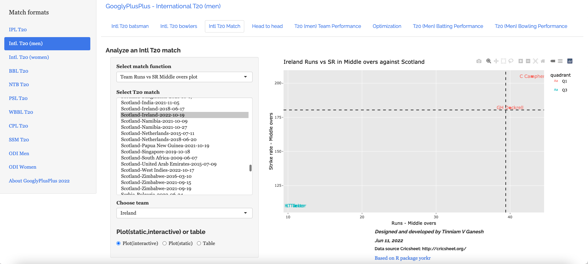
5.Scotland vs Ireland – 19 Oct 2022 : Team Runs vs SR Middle overs plot
Curtis Campher snatched the game away from Scotland with his stellar performance in middle and death overs
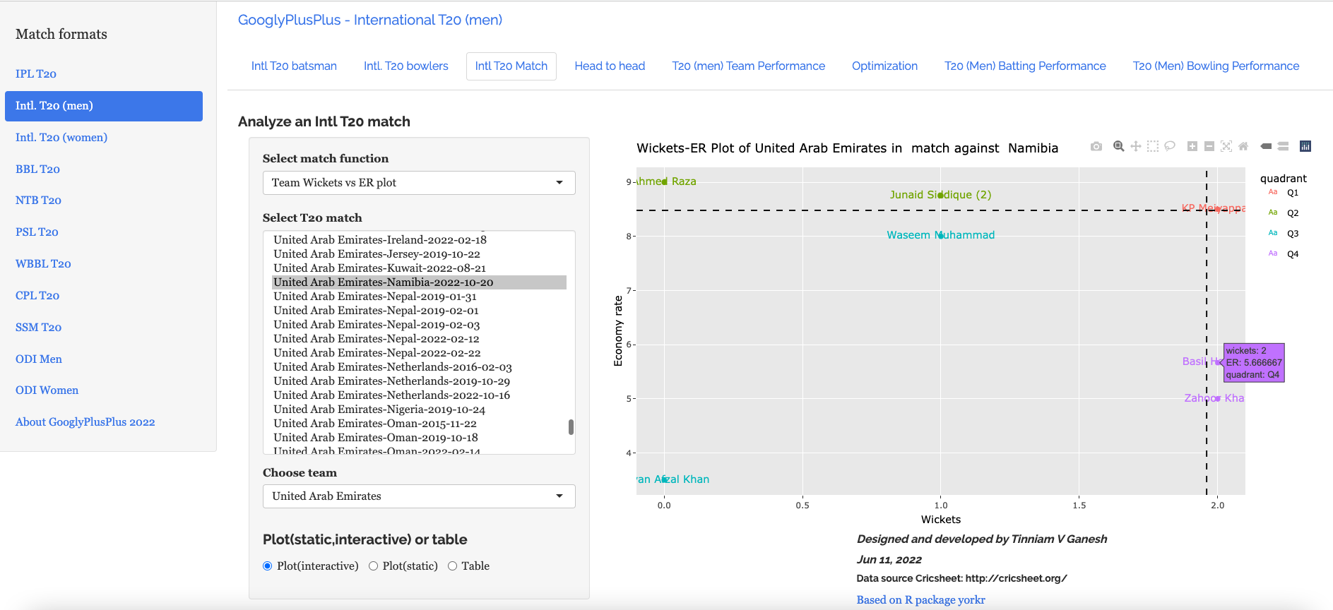
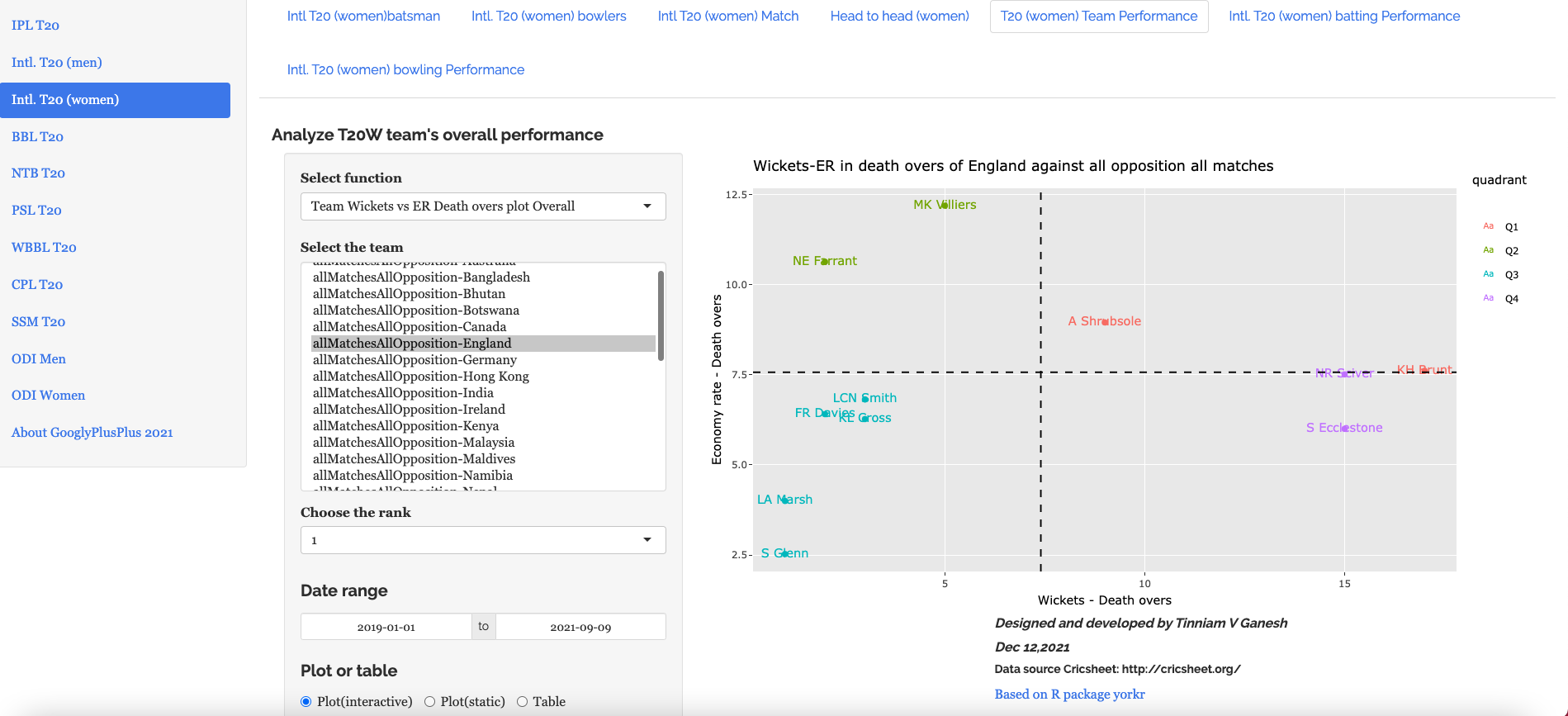
6. UAE vs Namibia : 20 Oct 2022 : Team Wickets vs ER plot
Basoor Hameed and Zahoor Khan got 2 wickets apiece with an economy rate of ~5.00 but still they were not able to stop UAE from stealing a win
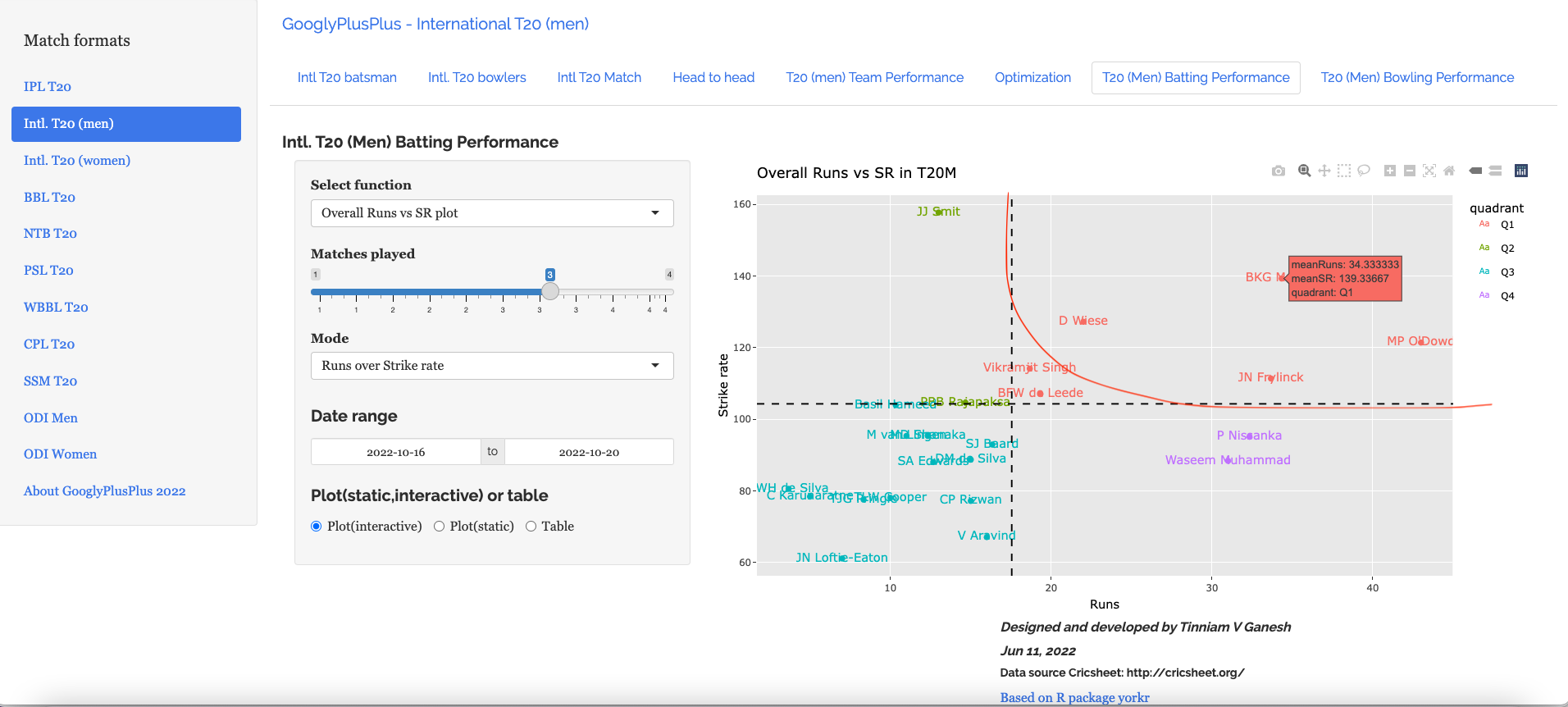
7. Overall Runs vs SR in T20 World Cup 2022
It is too early to rank the players, nevertheless in the current T20 World Cup, MP O’Dowd (Netherlands), BKG Mendis (Sri Lanka) and JN Frylinck(Namibia) are the top 3 batsmen with good runs and Strike Rate
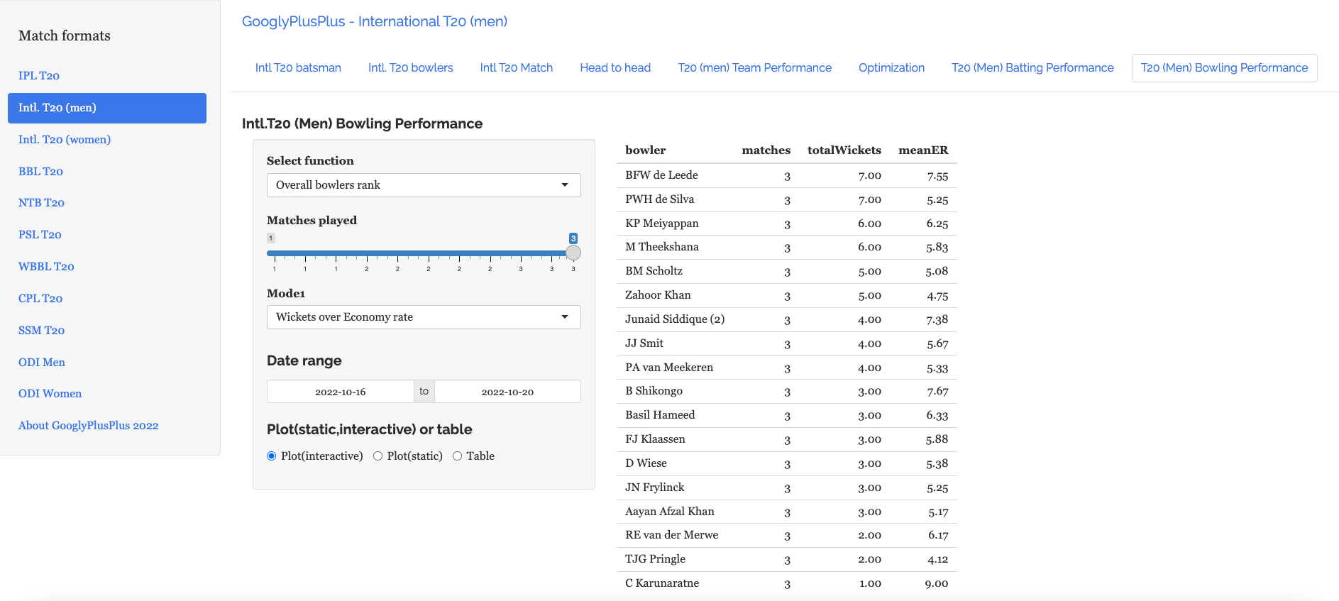
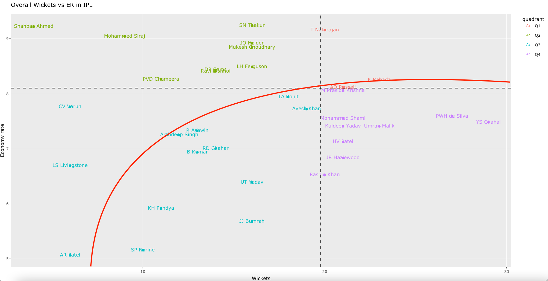
8. Overall Wickets over ER in T20 World Cup 2022
The top 3 bowlers so far in T20 World Cup 2022 are a) BFW de Leede (Netherlands) b) PWH De Silva (Sri Lanka) c) KP Meiyappan (UAE) with a total of 7,7, and 6 wickets respectively
Note: Besides the match analysis GooglyPlusPlus also provides detailed analysis of batsmen, bowlers, matches as above, team-vs-team, team-vs-all teams, ranking of batsmen & bowlers etc. For more details see my post GooglyPlusPlus gets ready for ICC Men’s T20 World Cup
Do visit GooglyPlusPlus everyday to check out the cricketing actions of matches gone by. You can also follow me on twitter @tvganesh_85 for daily highlights.
It is time!! So last weekend, I turned the wheels, moved the levers and listened to the hiss of steam, as I cranked up my Shiny app GooglyPlusPlus. The ICC Men’s T20 World Cup is just around the corner, and it was time to prepare for this event. This latest GooglyPlusPlus is current with the latest Intl. men’s T20 match data, give or take a few. GooglyPlusPlus can analyze batsmen, bowlers, matches, team-vs-team, team-vs-all teams, besides also ranking batsmen, bowlers and plot performances in Powerplay, middle and death overs.
In this post, I include a quick refresher of some of features of my app GooglyPlusPlus. Note: This is a random sampling of the functions available. There are more than 120+ features available in the app.
Check out your favourite players and your country’s team with GooglyPlusPlus
Note 1: All charts are interactive
Note 2: You can choose a date range for your analysis
Note 3: The data for this app is taken from Cricsheet
T20Batsman tab
This tab includes functions pertaining to individual batsmen. Functions include Runs vs Deliveries, moving average runs, cumulative average run, cumulative average strike rate, runs against opposition, runs at venue etc.
For e.g.
a) Suryakumar Yadav’s (India) cumulative strike rate
b) Mohammed Rizwan’s (Pakistan) performance against opposition
2. T20 Bowler’s Tab
The bowlers tab has functions for computing mean economy rate, moving average wickets, cumulative average wicks, cumulative economy rate, bowlers performance against opposition, bowlers performance in venue, predict wickets and others
A random function is shown below
a) Predict wickets for Wanindu Hasaranga of Sri Lanka
3. T20 Match tab
The match tab has functions that can compute match batting & bowling scorecard, batting partnerships, batsmen performance vs bowlers, bowler’s wicket kind, bowler’s wicket match, match worm graph, match worm wicket graph, team runs across 20 overs, team wickets in 20 overs, teams runs or wickets in powerplay, middle and death overs
Here are a couple of functions from this tab
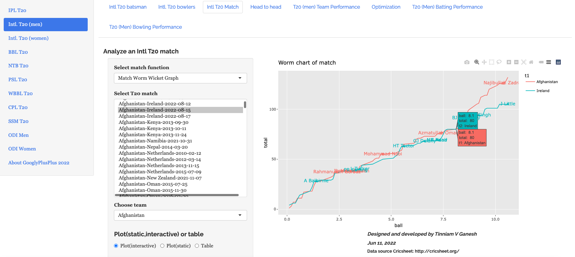
a) Afghanistan vs Ireland – 2022-08-15
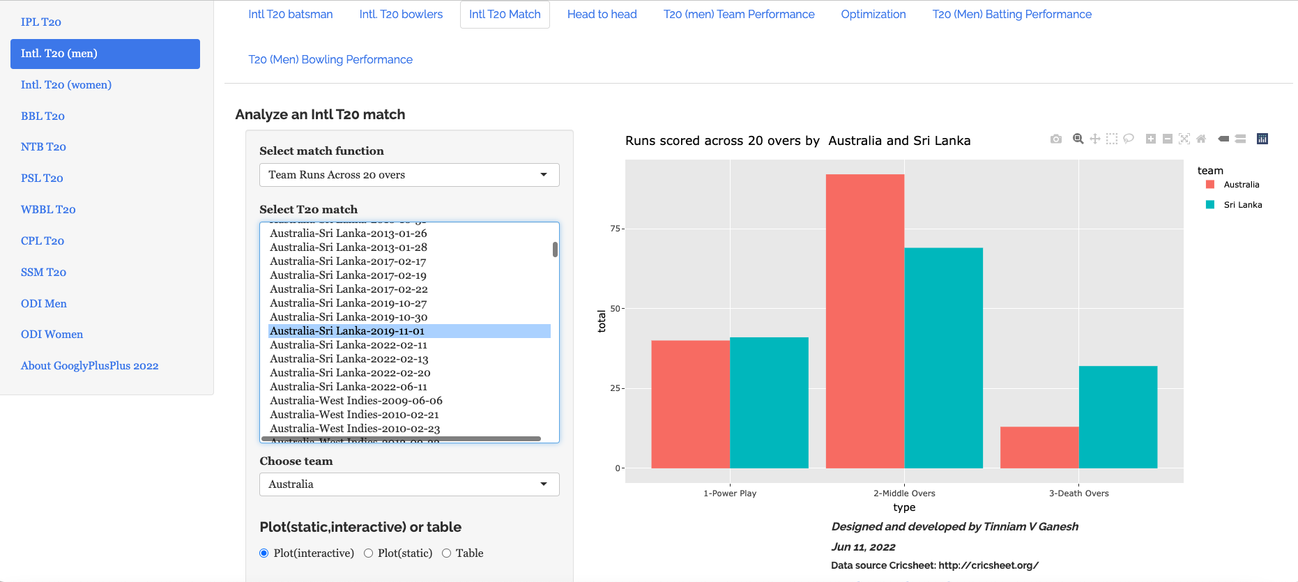
b) Australia vs Sri Lanka – 2019-11-01 – Runs across 20 overs
4. T20 Head-to-head tab
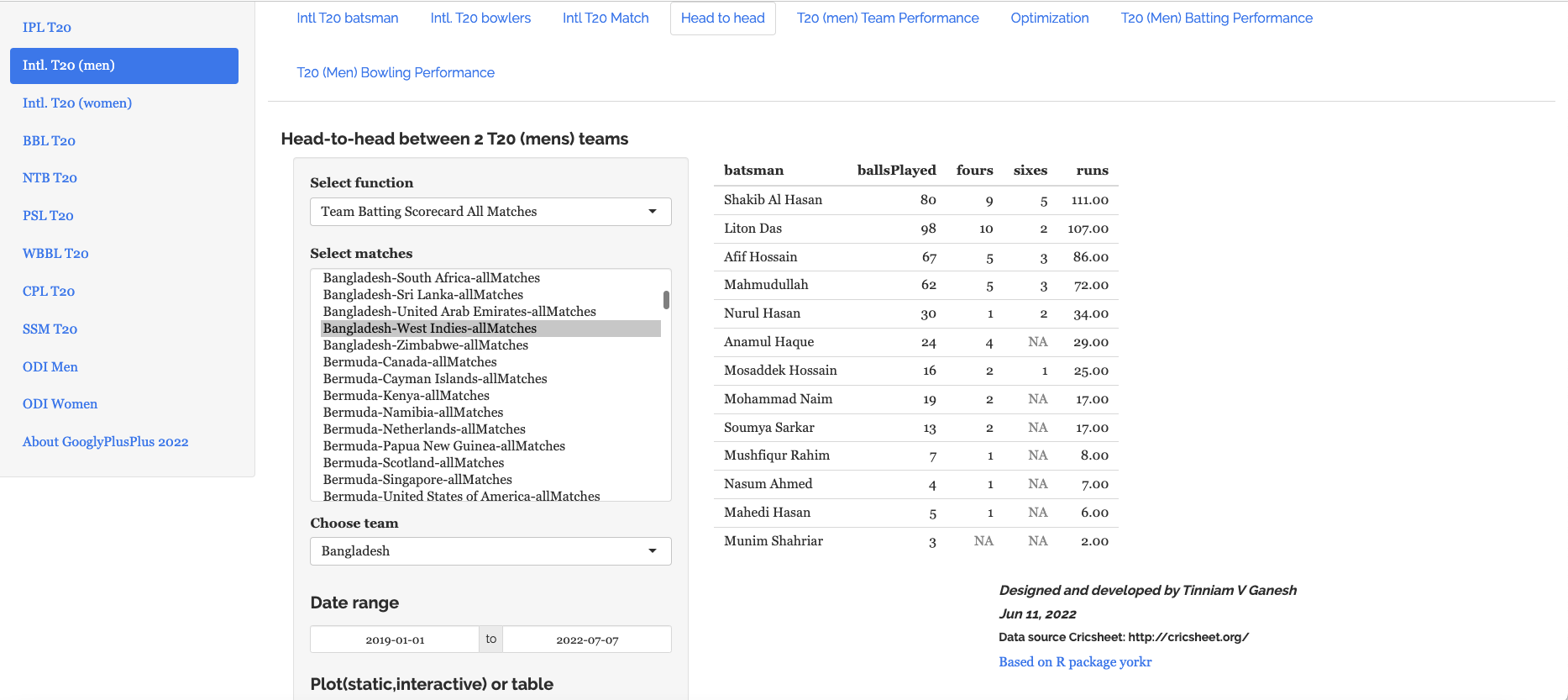
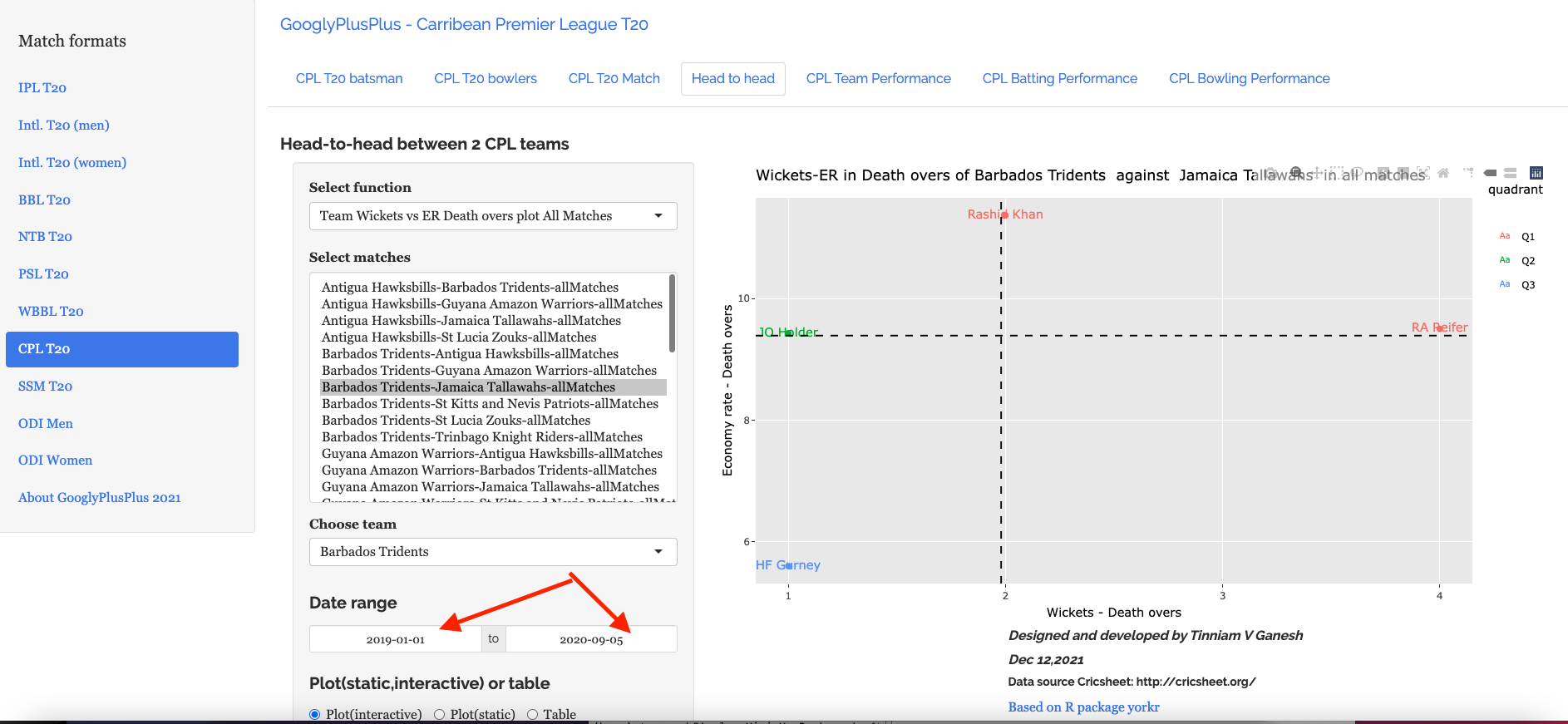
This tab provides the analysis of all combination of T20 teams (countries) in different aspects. This tab can compute the overall batting, bowling scorecard in all matches between 2 countries, batsmen partnerships, performances against bowlers, bowlers vs batsmen, runs, strike rate, wickets, economy rate across 20 overs, runs vs SR plot and wicket vs ER plot in all matches between team and so on. Here are a couple of examples from this tab
a) Bangladesh vs West Indies – Batting scorecard from 2019-01-01 to 2022-07-07
b) Wickets vs ER plot – England vs New Zealand – 2019-01-01 to 2021-11-10
5. T20 Team performance overalltab
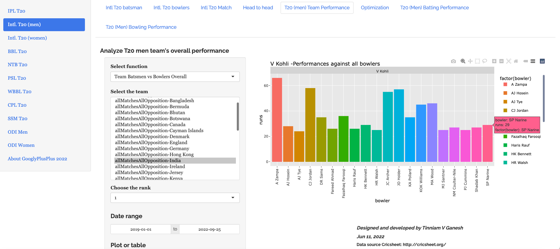
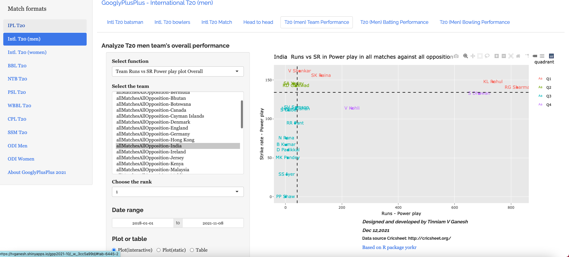
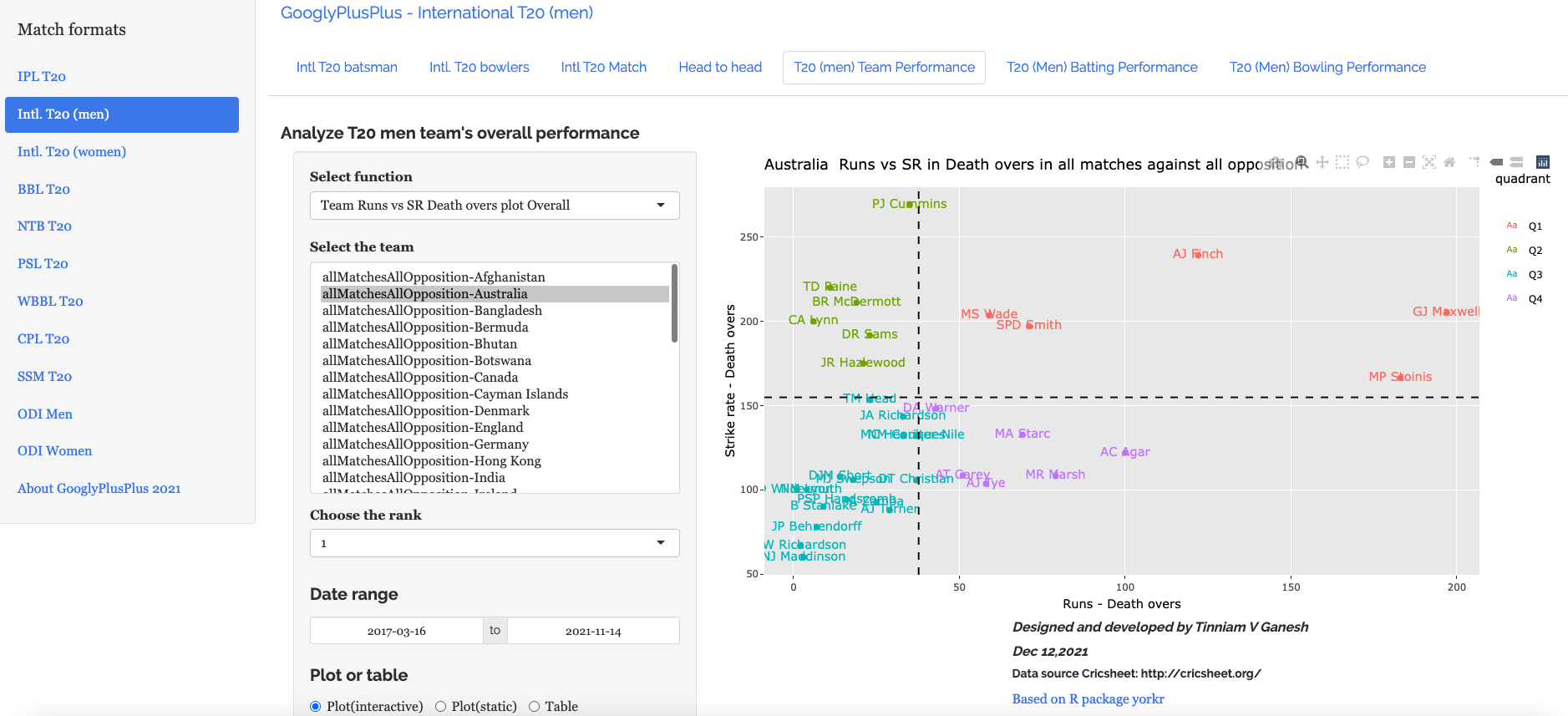
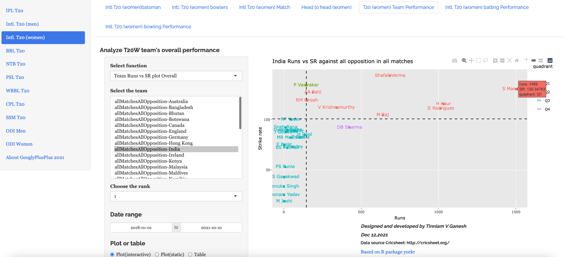
This tab provides detailed analysis of the team’s performance against all other teams. As in the previous tab there are functions to compute the overall batting, bowling scorecard of a team against all other teams for any specific interval of time. This can help in picking out the most consistent batsmen, bowlers. Besides there are functions to compute overall batting partnerships, bowler vs batsmen, runs, wickets across 20 overs, run vs SR and wickets vs ER etc.
a) Batsmen vs Bowlers (Rank 1- V Kohli 2019-01-01 to 2022-09-25)
b) team Runs vs SR in Death overs (India) (2019-01-01 to 2022-09-25)
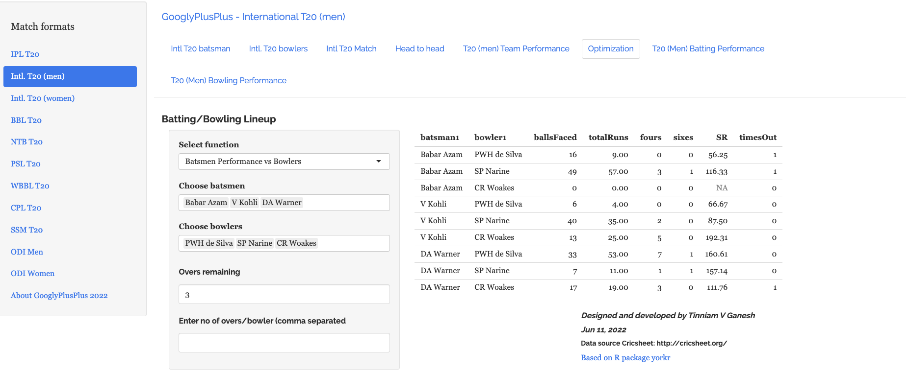
6) Optimisation tab
In the optimisation tab we can check the performance of a specific batsmen against specific bowlers or bowlers against batsmen
a) Batsmen vs Bowlers
b) Bowlers vs batsmen
7) T20 Batting Performancetab
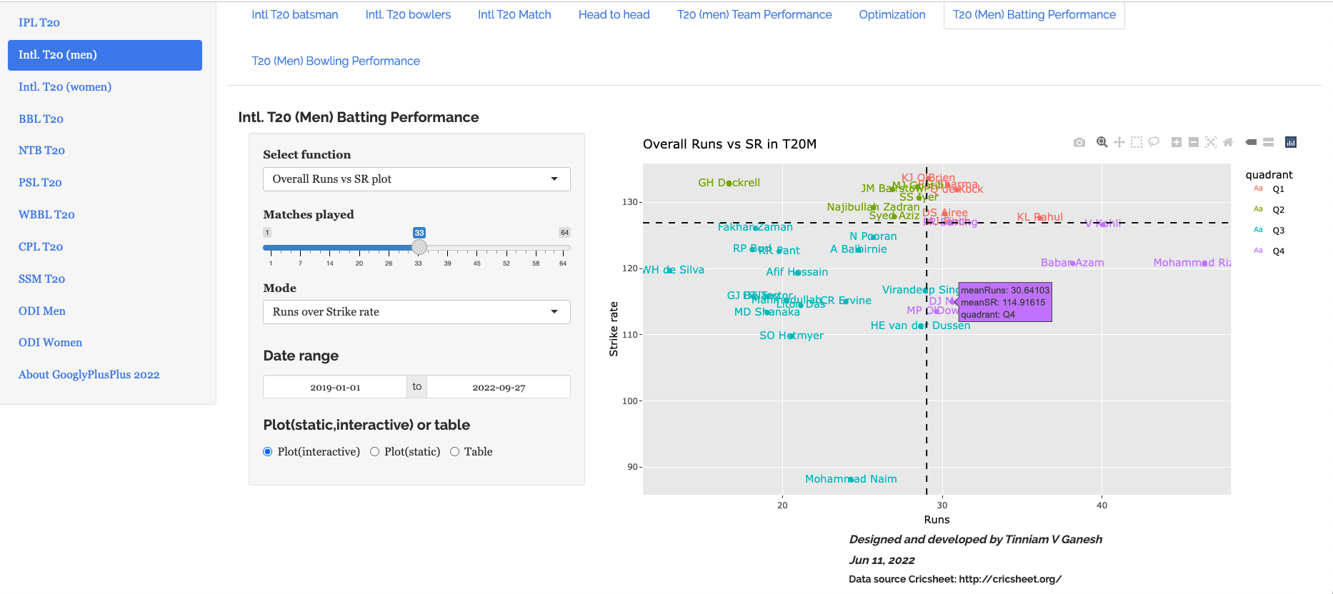
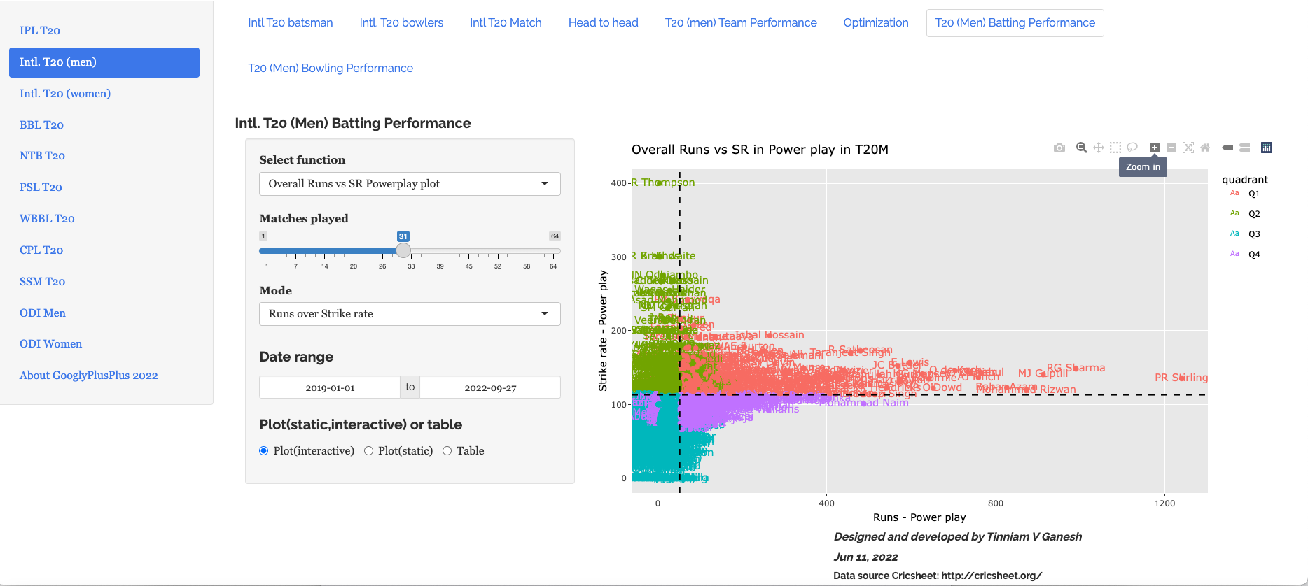
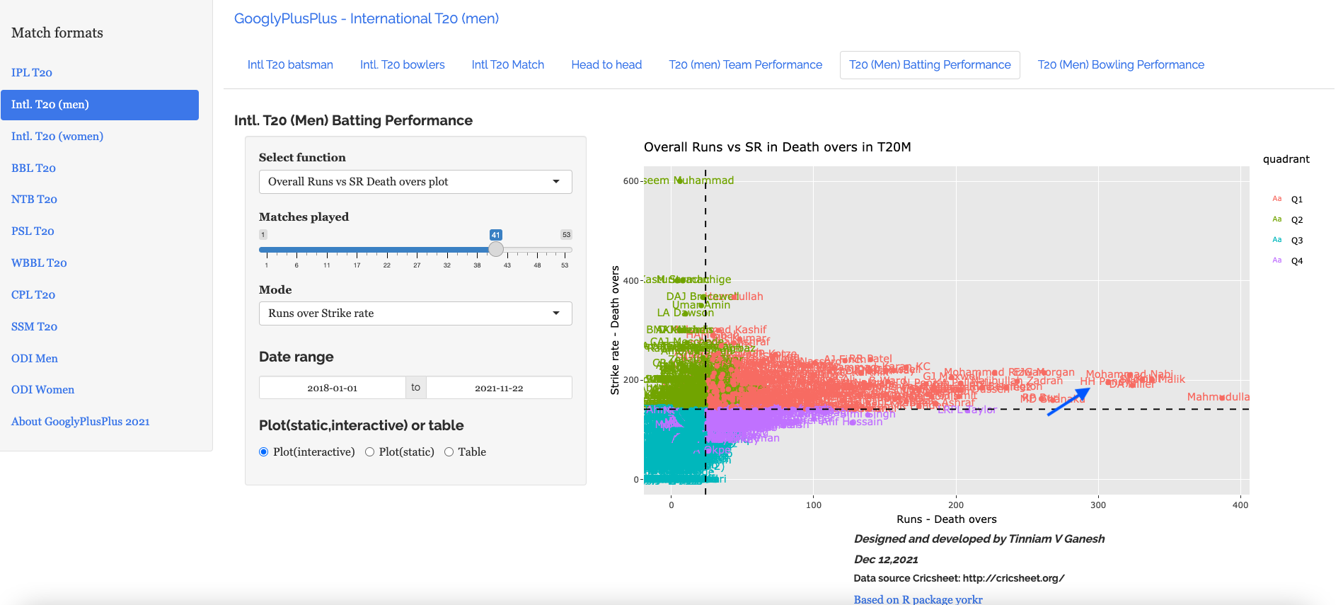
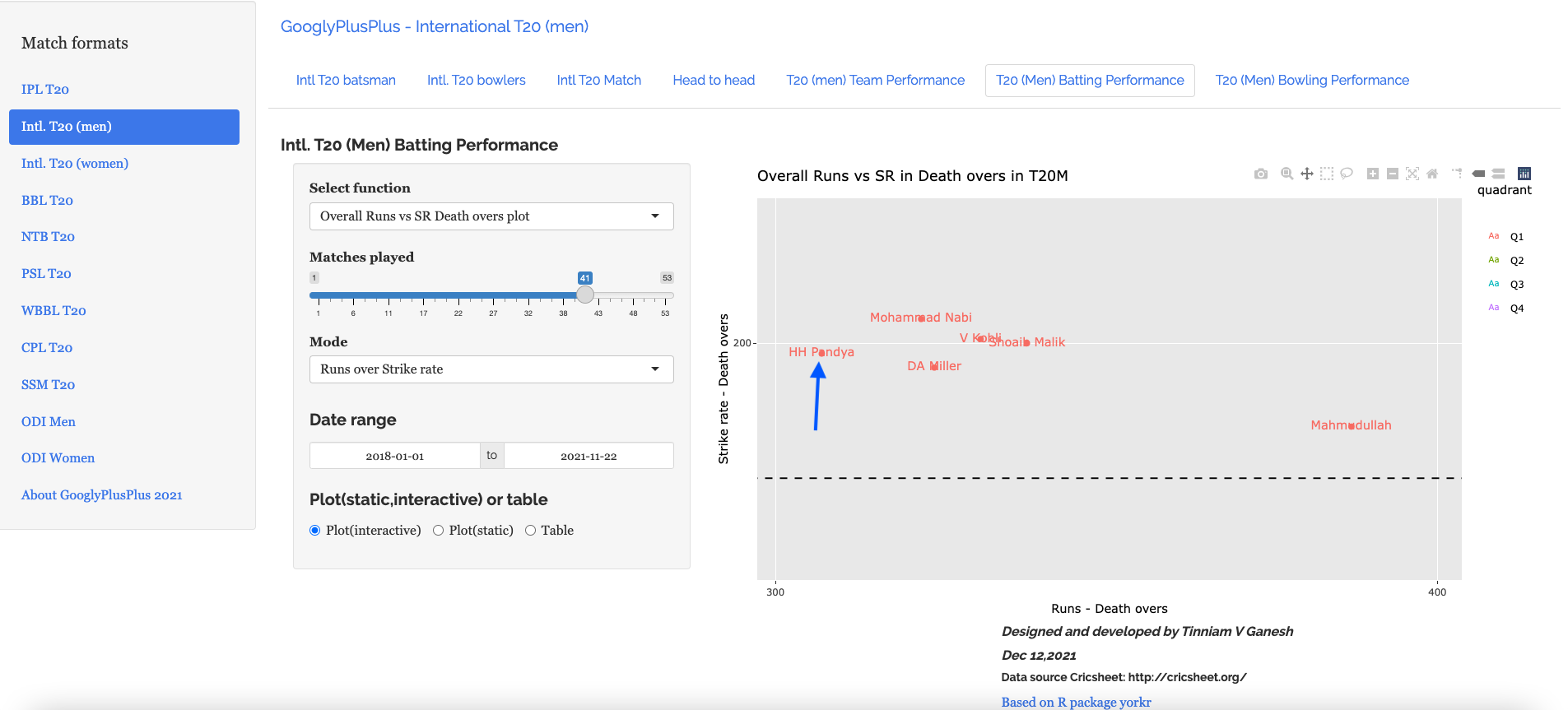
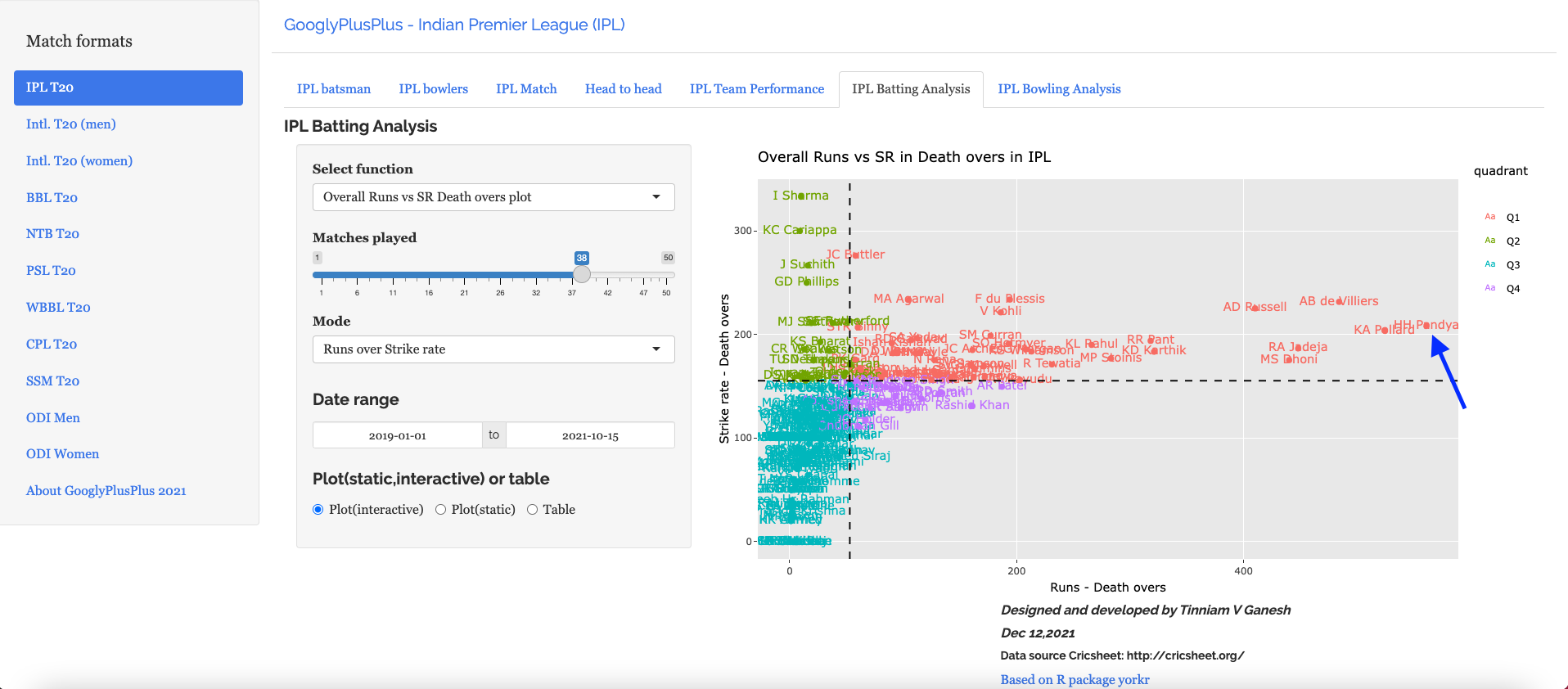
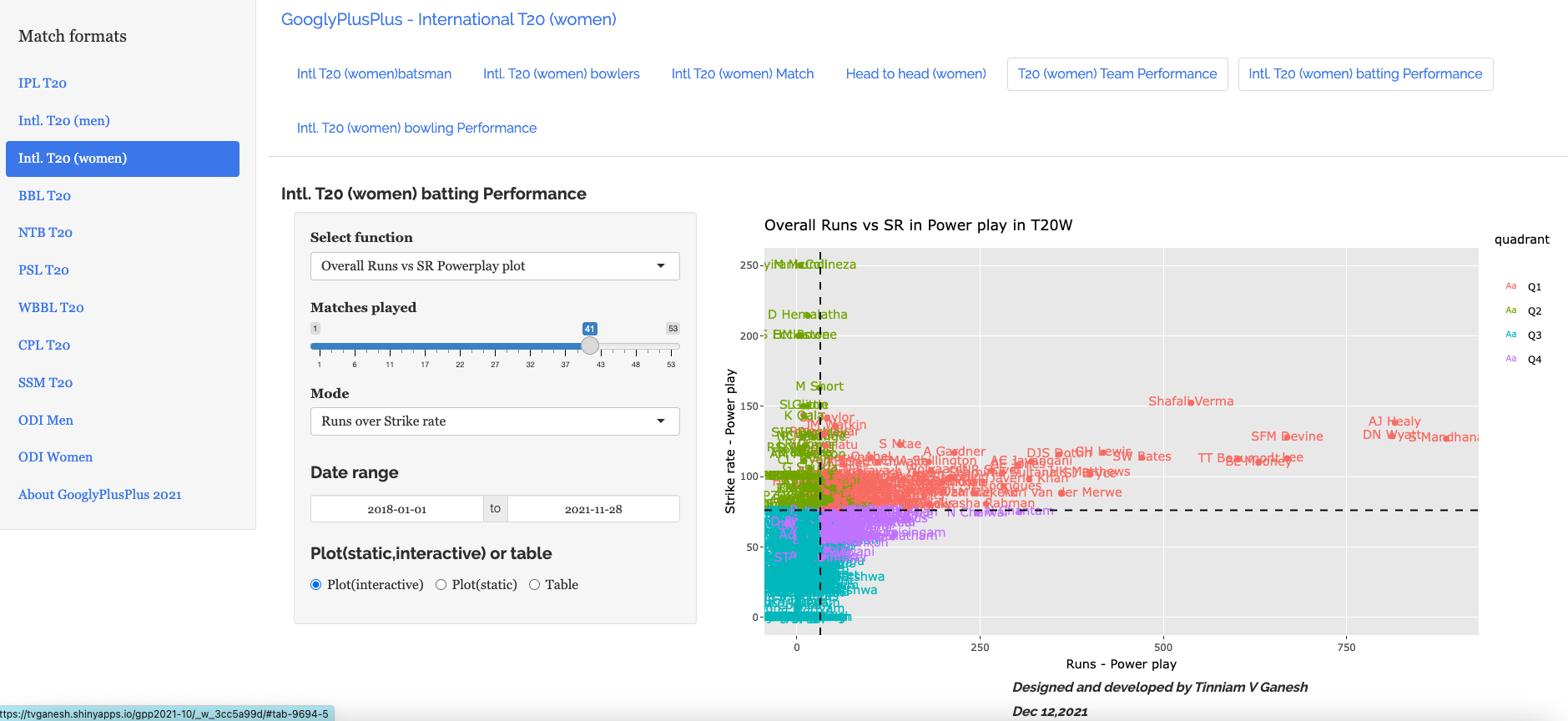
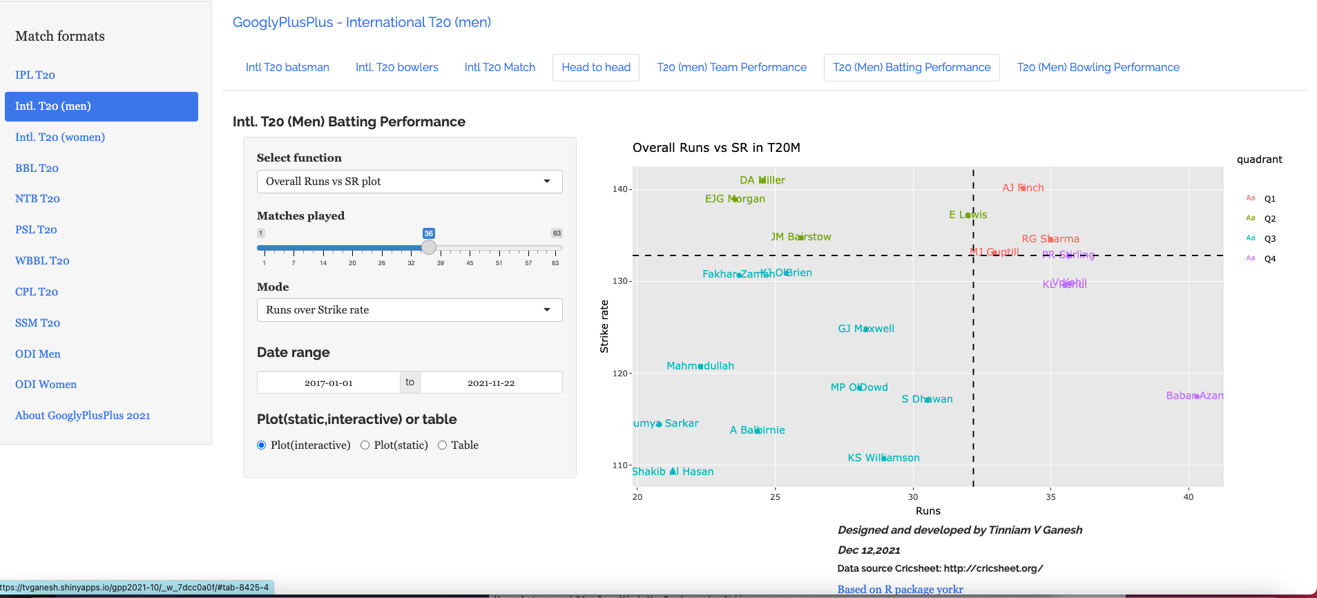
This tab performs various analytics like ranking batsmen based on Run over SR and SR over Runs. Also you can plot overall Runs vs SR, and more specifically Runs vs SR in Powerplay, Middle and Death overs. All of this can be done for a specific date range. Here are some examples. The data includes all of T20 (all countries all matches)
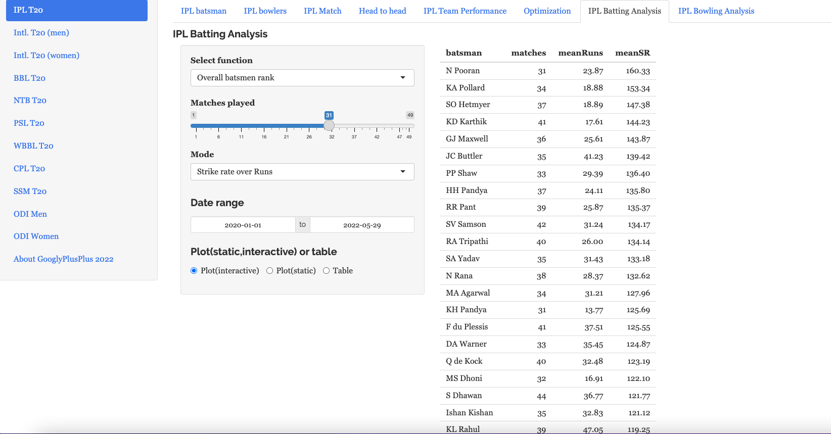
a) Rank batsmen (Runs over SR, minimum matches played=33, date range=2019-01-01 to 2022-09-27)
The top 3 batsmen are Mohamen Rizwan, V Kohli and Babar Azam
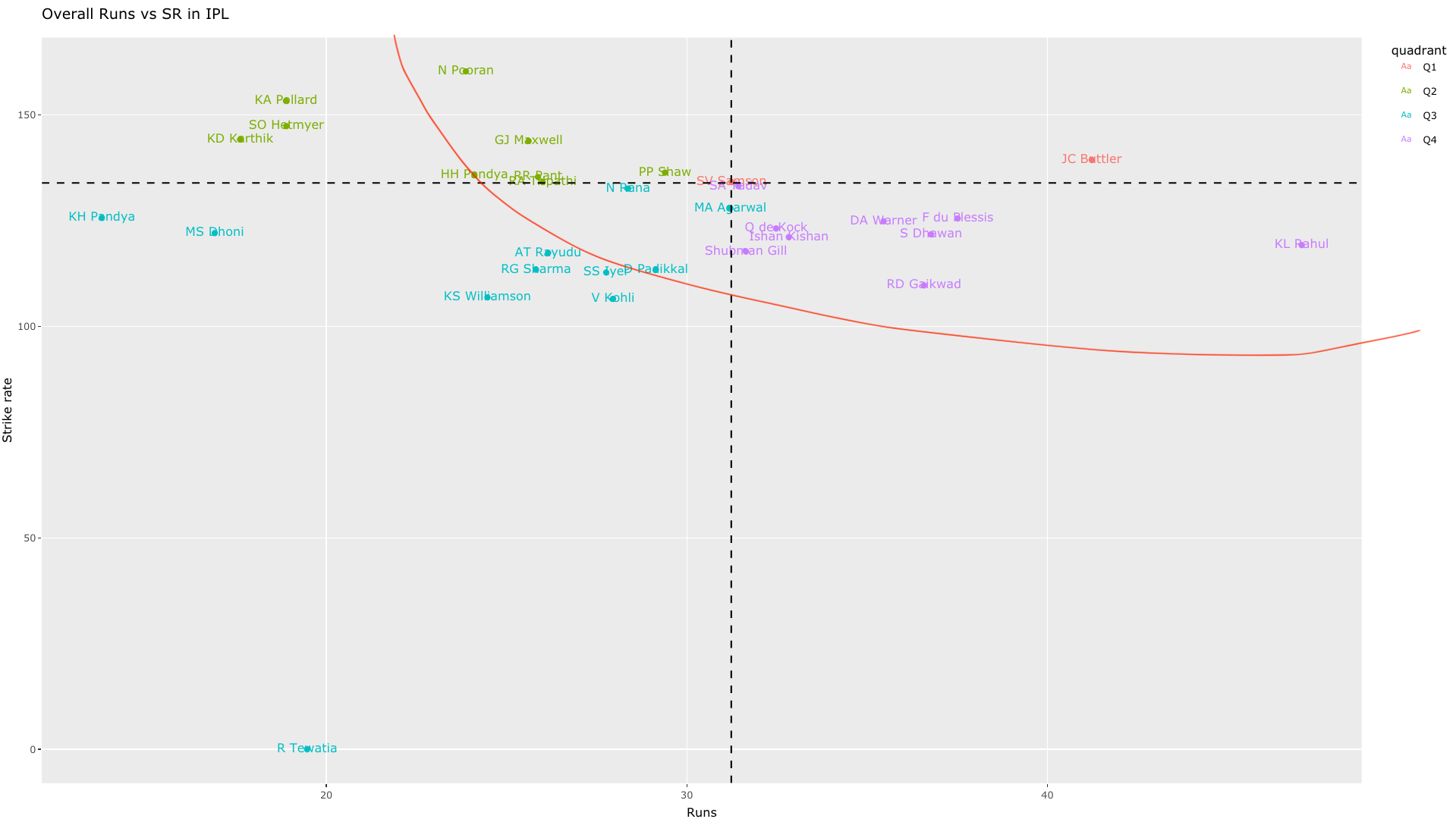
b) Overall runs vs SR plot (2019-01-01 to 2022-09-27)
c) Overall Runs vs SR in Powerplay (all teams- 2019-01-01-2022-09-27)
This plot will be crowded. However, we can zoom into an area of interest. The controls for interacting with the plot are in the top of the plot as shown
Zooming in and panning to the area we can see the best performers in powerplay are as below
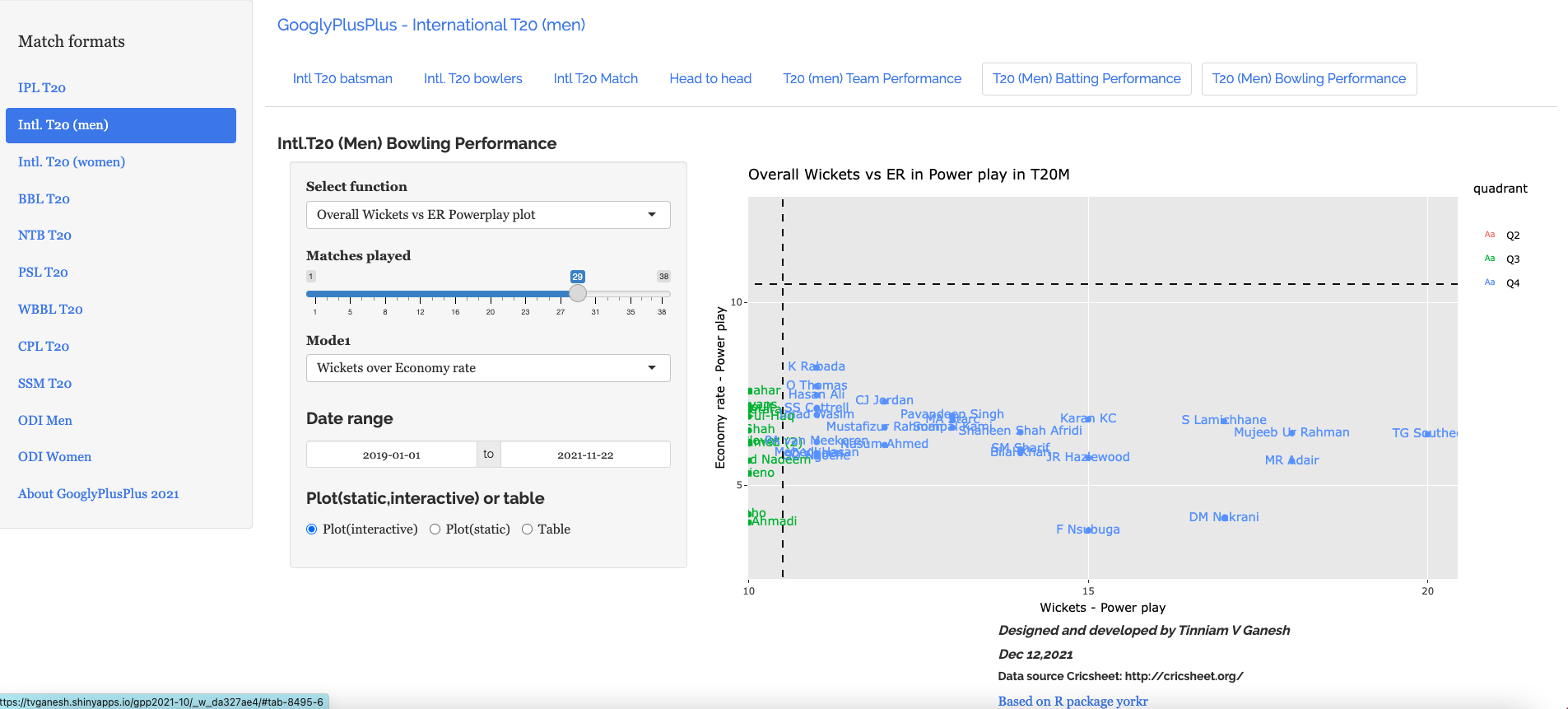
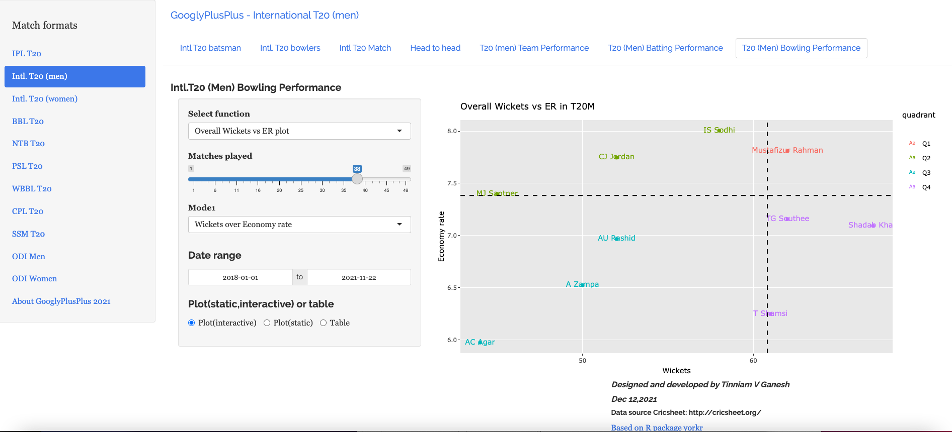
8) T20 Bowling Performancetab
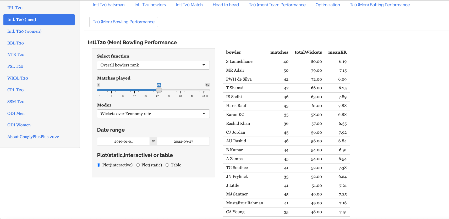
This tab computes and ranks bowlers on Wickets over Economy and Economy rate over wickets. We can also compute and plot the Wickets vs ER in all matches , besides the Wickets vs ER in powerplay, middle and death overs with data from all countries
a) Rank Bowlers (Wickets over ER, minimum matches=28, 2019-01-01 to 2022-09-27)
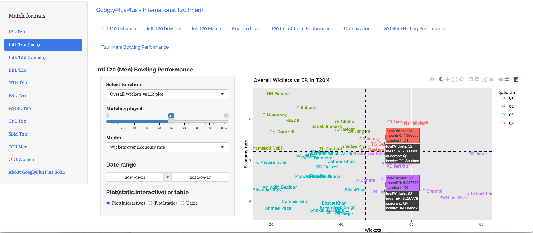
b) Wickets vs ER plot
S Lamichhane (NEP), Hasaranga (SL) and Shamsi (SA) are excellent bowlers with high wickets and low ER as seen in the plot below
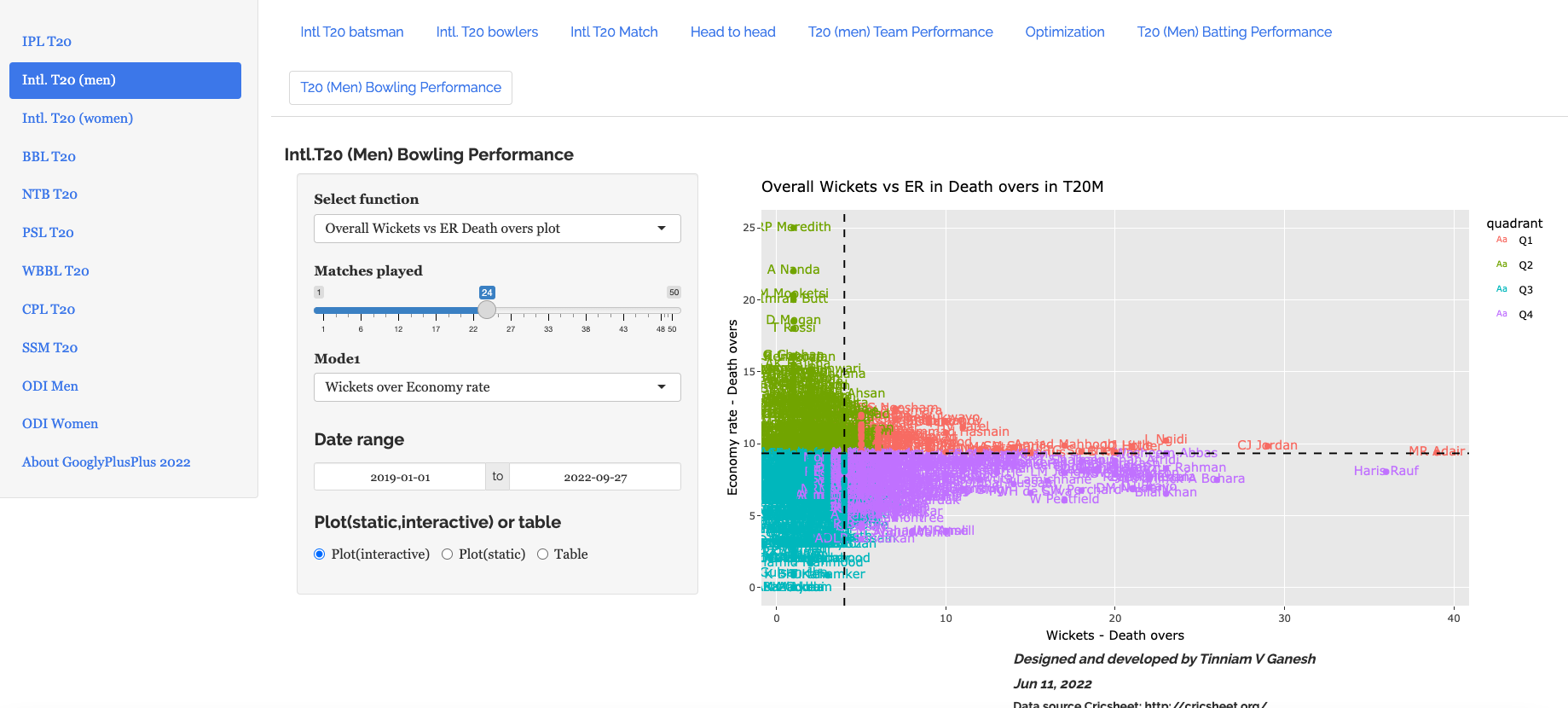
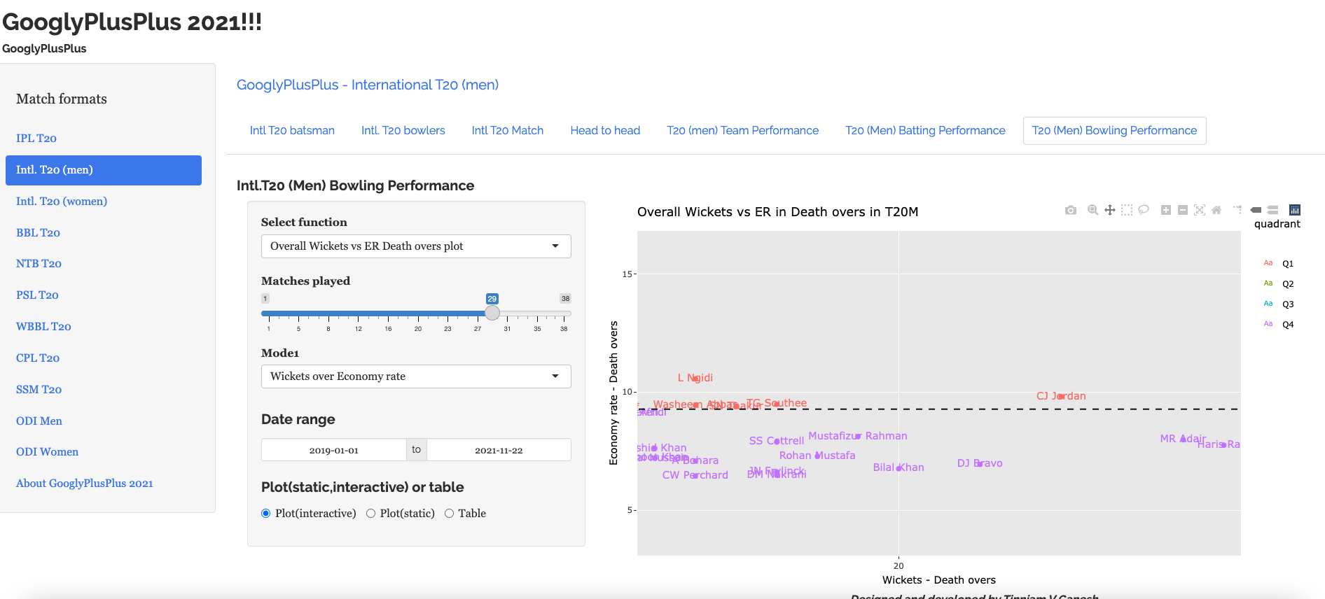
c) Wickets vs ER in death overs (2019-01-01 to 2022-09-27, min matches=24)
Zooming in and panning we see the best performers in death overs are MR Adair (IRE), Haris Rauf(PAK) and Chris Jordan (ENG)
With the excitement building up, it is time you checked out how your country will perform and the players who will do well.
IPL 2022 has just concluded and yet again, it is has thrown a lot of promising and potential youngsters in its wake, while established players have fallen! With IPL 2022, we realise that “Sceptre and Crownmusttumble down” and that ‘theglories‘ of form and class like everything else are “shadows not substantial things” (Death the Leveller by James Shirley).
So King Kohli had to kneel, and hitman’ himself got hit. Rishabh Pant, Jadeja also had a poor season. On the contrary there were several youngsters who shone like Abhishek Sharma, Tilak Verma, Umran Malik or a Mohsin Khan
This post is about my potential T20 Indian players for the World Cup 2022 and beyond.
The post below includes my own analysis and thoughts. Feel free to try out my Shiny app GooglyPlusPlus and draw your own conclusions.
How often we hear that data by itself is useless, unless we can draw insights from it? This is a prevailing theme in the corporate world and everybody uses all sorts of tools to analyse and subsequently draw insights. Data analysis can be done in many ways as data can be sliced, diced, chopped in a zillion ways. There are many facets and perspectives to analysing data. Creating insights is easy, but arriving at actionable insights is anything but. So, the problem of selecting the best 11 is difficult as there are so many ways to look at the analysis. My Shiny app GooglyPlusPlus based on my R package yorkr can analyse data in several ways namely
Batsman analysis
Bowler analysis
Match analysis
Team vs team analysis
Team vs all teams analysis
Batsman vs bowler and vice versa
Analysis of in 3,4,5 in power play, middle and death overs
GooglyPlusPlus uses my R package yorkr which has ~ 160 functions some which have several options. So, we can say roughly there are ~500 different ways that analysis can be done or in other words we can gather almost roughly 500+ different insights, not to mention that there are so many combinations of head-on matches and one-vs-all matches.
So generating insights or different ways of analysis data alone is not enough. The question is whether we can get a consolidated view from the different insights. In this post, I try to identify the best contenders for the Indian T20 team. This is far more difficult than it looks. Do you select players on past historical performance or do you choose from the newer crop of players, who have excelled in the recent IPL season. I think this boils down the typical situation in any domain. In engineering, we have tradeoffs – processing power vs memory tradeoff, throughput vs latency tradeoff or in the financial domain it is cost vs benefit or risk vs reward tradeoff. For team selection, the quandary is, whether to choose seasoned players with good historical performance but a poor performances in recent times or go with youngsters who have played with great courage and flair in this latest episode of IPL 2022. Hence there is a tradeoff between reliable but below average performance or risky but superlative performances of new players.
For this I base my potential list from
Then (past history of batsmen & bowlers) – I have chosen the performance of batsmen and bowlers in the last 3 years. With we can arrive at those who have had reasonably reliable performance for the last 3 years
Now (IPL 2022) – Performance in the current season IPL 2022
A. Then (Jan 2020 – May 2022) – Batsmen analysis
In this section I analyse the performances of batsmen and bowlers from Jan 2022 – May 2022. This is done based on ranking, and plots of Runs vs Strike Rate in Power Play, Middle and Death overs
Also I analyse bowlers based on the overall rank from Jan 2022- May 2022. Further more analysis is done on Wickets vs Economy Rate overall and in Power Play, Middle and Death overs
a. Ranks of batsmen (Runs over Strike Rate) : Jan 2020 – May 2022
IPL 2022 just finished and clearly brings out the batsmen who are in great nick. It is always going to be a judgment call of whether to go for ‘old reliable’ or ‘new and awesome’.
a. Ranks of batsmen (Runs over Strike Rate) : IPL 2022
The best batsmen this season in Runs over Strike rate are
f. Best batsmen Runs vs SR in Death overs:IPL 2022
Top batsmen in death overs in IPL 2022
[Dinesh Karthik, Rahul Tewatia, MS Dhoni, KL Rahul, Azar Patel, Washington Sundar, R Ashwin, Hardik Pandya, Ayush Badoni, Shivam Dube, Suryakumar Yadav, Ravindra Jadeja, Sanju Samson]
OverallBattingPerformance in season
Kohli peaked in 2016 and from then on it has been a downward slide (see below)
Taking a look at Kohli’s moving average it is clear that he is past his prime and it will take a herculean effort to regain his lost glory
Similarly, Rohit Sharma’s moving average is constantly around ~30 as seen below
The cumulative average of Rohit Sharma is shown below
Comparing KL Rahul, Shikhar Dhawan, Rohit Sharma and V Kohli we see that KL Rahul and Shikhar Dhawan have had a much superior performance in the last 2-3 years. Rohit has averaged about ~25 runs every season.
Comparing the 4 wicket-keeper batsmen Sanju Samson, Rishabh Pant, Ishan Kishan and Dinesh Karthik from 2016
i) Runs over Strike Rate
We see that Pant peaked in 2018 but has not performed as well since. In the last 2 years Sanju Samson and Ishan Kishan have done well
ii) Strike Rate over Runs
For the last couple of seasons Rishabh Pant and Dinesh Kartik top the strike rate over the other 2
Similar analysis can be done other combinations of batsmen
Choosing the best batsmen from the above, my top 5 batsmen would be
Personally, I feel Ishan Kishan and Shreyas Iyer are a little tardy while playing express speeds, as compared to Sanju Samson or Rishabh Pant.
If you notice, I have not included both Virat Kohli or Rohit Sharma who have been below par for some time
C.Then (Jan 2020 – May 2022) – Bowler analysis
This section I analyse the performances of bowlers from Jan 2022 – May 2022. This is done based on ranking, and plots of Wickets vs Economy Rate in Power Play, Middle and Death overs
a. Ranks of bowlers (Wickets over Economy Rate) : Jan 2020 – May 2022
The most consistent bowlers Wickets over Economy Rate for the last 3 years are
[YS Chahal, Jasprit Bumrah, Mohammed Dhami, Harshal Patel, Shardul Thakur, Arshdeep Singh, Rahul Chahar, Varun Chakravarthy, Ravi Bishnoi, Prasidh Krishna, R Ashwon, Axar Patel, Mohammed Siraj, Ravindra Jadeja, Krunal Pandya, Rahul Tewatia]
b. Ranks of bowlers (Economy Rate over Wickets) : Jan 2020 – May 2022
The most economical bowlers since 2020 are
[Axar Patel, Krunal Pandya, Jasprit Bumrah, CV Varun, R Ashwin, Ravi Bishnoi, Rahul Chahar, YS Chahal, Ravindra Jadeja, Harshal Patel, Mohammed Shami, Mohammed Siraj, Rahul Tewatia, Arshdeep Singh, Prasidh Krishna, Shardul Thakur]
c.BestBowlers Wickets vs ER :Jan 2020 – May 2022
The best bowlers Wickets vs ER will be in the bottom right quadrant. The most consistent and reliable bowlers are
[YS Chahal, Jasprit Bumrah, Mohammed Shami, Harshal Patel, CV Arun, Ravi Bishnoi, Rahul Chahar, R Ashwin, Axar Patel]
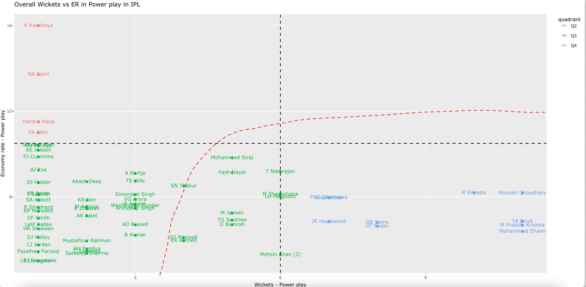
d. Best bowlers Wickets vs ER in Powerplay:Jan 2020 – May 2022
The best bowlers in Powerplay are
[Mohammed Shami, Deepak Chahar, Mohammed Siraj, Arshdeep Singh, Jasprit Bumrah, Avesh Khan, Mukesh Choudhary, Shardul Thakur, T Natarajan, Bhuvaneshwar Kumar, WashingtonSundar, Shivam Mavi]
e. Best bowlers Wickets vs ER in Middle overs : Jan 2020 – May 2022
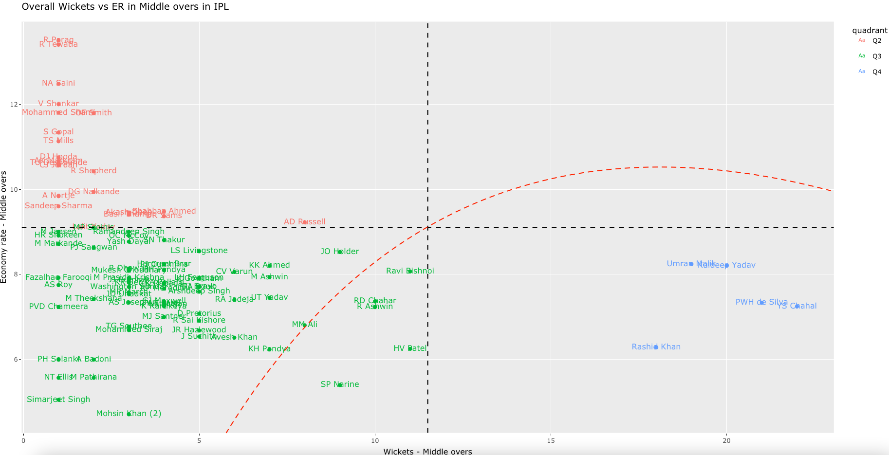
The most reliable performers in middle overs from 2020-2022 are
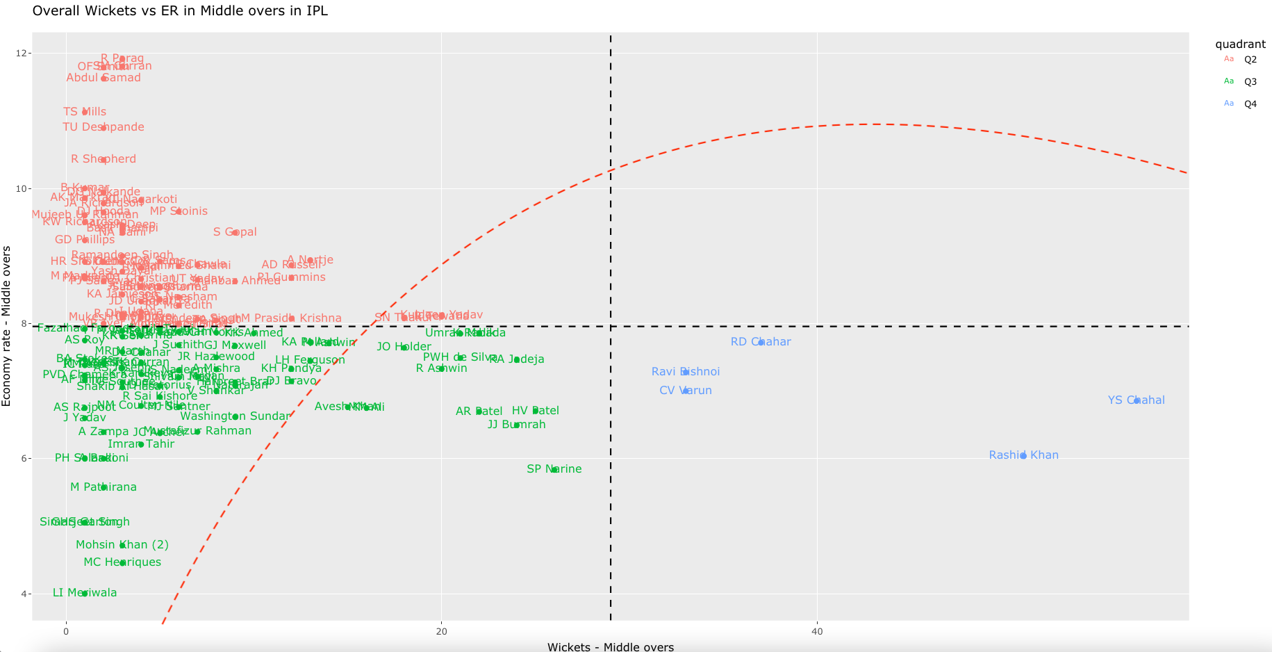
[YS Chahal, Rahul Chahr, Ravi Bishnoi, Harshal Patel, Axar Patel, Jasprit Bumrah, Umran Malik, R Ashwin, Avesh Khan, Shardul Thakur, Kuldeep Yadav]
f. Best bowlers Wickets vs ER in Death overs : Jan 2020 – May 2022
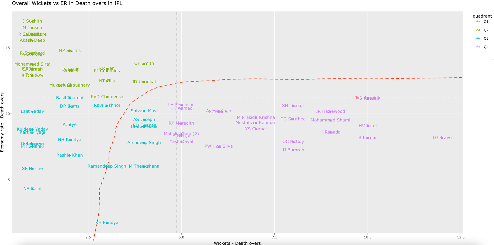
The most reliable bowlers are
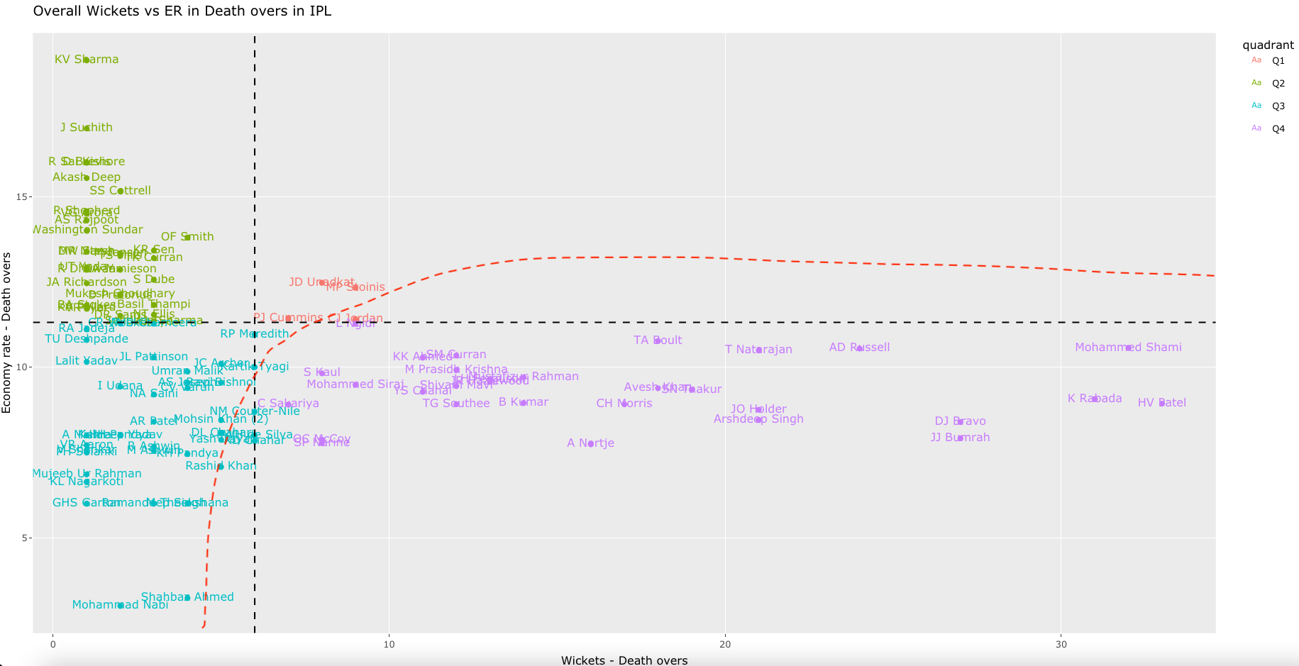
[Harshal Patel, Mohammed Shami, Jasprit Bumrah, Arshdeep Singh, T Natarajan, Avesh Khan, Shardul Thakur, Bhuvaneshwar Kumar, Shivam Mavi, YS Chahal, Prasidh Krishna, Mohammed Siraj, Chetan Sakariya]
B) Now (IPL 2022)– Bowler analysis
a. Ranks of bowlers (Wickets over Economy Rate) : IPL 2022
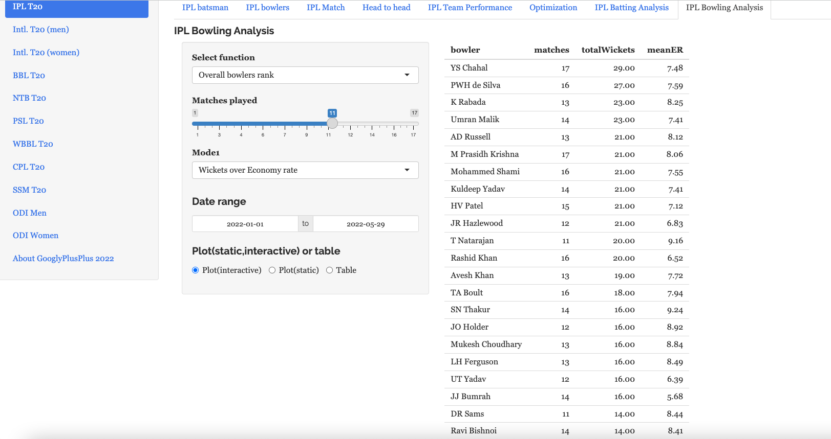
The best bowlers in IPL 2022 when considering Wickets over Economy Rate
[YS Chahal, Umran Malik, Prasidh Krishna, Mohammed Shami, Kuldeep Yadav, Harshal Patel, T Natarajan, Avesh Khan, Shardul Thakur, Mukesh Choudhary, Jasprit Bumrah, Ravi Bishnoi]
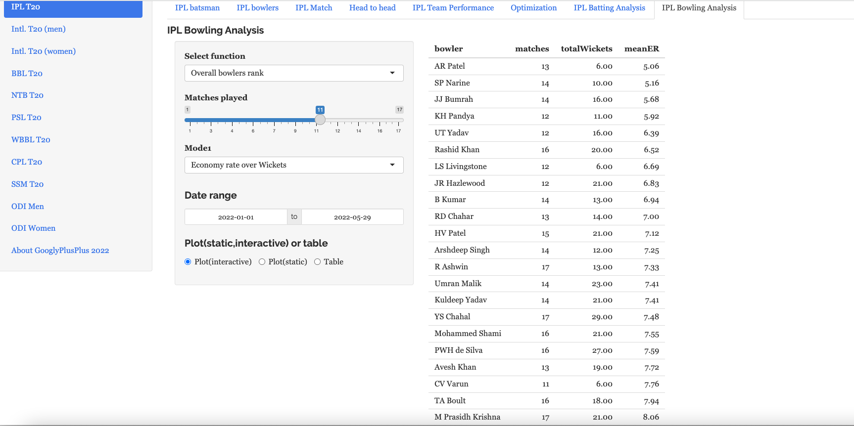
a. Ranks of bowlers (Economy Rate over Wickets) : IPL 2022
The most economical bowlers in IPL 2022 are
[Axar Patel, Jasprit Bumrah, Krunal Pandya, Umesh Yadav, Bhuvaneshwar Kumar, Rahul Chahr, Harshal Patel, Arshdeep Singh, R Ashwion, Umran Malik, Kuldeep Yadav, YS Chahal, Mohammed Shami, Avesh Khan, Prasidh Krishna]
c.BestBowlers Wickets vs ER :IPL 2022
The overall best bowlers in IPL 2022 are
[YS Chahal, Umran Malik, Harshal Patel, Prasidh Krishna, Mohammed Shami, Kuldeep Yadav, Avesh Khan, Jasprit Bumrah, Umesh Yadav, Bhuvaneshwar Kumar, Arshdeep Singh, R Ashwin, Rahul Chahar, Krunal Pandya]
d. Best bowlers Wickets vs ER in Powerplay: IPL 2022
The best bowlers in IPL 2022 in Power play are
[Mukesh Choudhary, Mohammed Shami, Prasidh Krishna, Umesh Yadav, Avesh Khan, Mohsin Khan, T Natarajan, Jasprit Bumrah, Yash Dayal, Mohammed Siraj]
d. Best bowlers Wickets vs ER in Middle overs: IPL 2022
The best bowlers in IPL 2022 during middle overs
The best bowlers are
[YS Chahal, Umran Malik, Kuldeep Yadav, Harshal Patel, Ravi Bishnoi, R Ashwin]
e. Best bowlers Wickets vs ER in Death overs: IPL 2022
The best bowlers in death overs in IPL 2022 are
[T Natarajan, Harshal Patel, Bhuvaneshwar Kumar, Mohammed Shami, Jasprit Bumrah, Shardul Thakur, YS Chahal, Prasidh Krishna, Avesh Khan, Mohsin Khan, Yash Dayal, Umran Malik, Arshdeep Singh]
Typically in a team we would need a combination of 4 bowlers (2 fast & 2 spinner or 3 fast and 1 spinner) with an additional player who is all rounder.
For 4 bowlers we could have
JJ Bumrah
Mohammed Shami, Umran Malik, Bhuvaneshwar Kumar, Umesh Yadav
Arshdeep Singh, Avesh Khan, Mohsin Khan, Harshal Patel
YS Chahal, Ravi Bishnoi, Rahul Chahar, Axar Patel
Ravindra Jadeja, Hardik Pandya, Rahul Tewathia, R Ashwin
i) Performance comparison (Wickets over Economy Rate)
Bumrah had the best season in 2020. He has been doing quite well and has been among the wickets
ii) Performance comparison (Economy Rate over Wickets)
Bumrah has the best Economy Rate
We can do a wicket prediction of bowlers. So for example for Bumrah it is
iii) Performance evaluation(Wickets over Economy Rate)
Harshal Patel followed by Avesh Khan had a good season last year, but Umran Malik pipped them this year (see below)
iv) Performance analysis of spinners
a. Wickets over Economy Rate: 2022
Chahal has the best season followed by Bishnoi and Chahar this season
b) Economy Rate over WIckets
Axar Patel has the best economy rate followed by Rahul Chahar
Conclusion
The above post identified the best candidates for the Indian team in the future and beyond. In my T20 list, I have neither included Virat Kohli or Rohit Sharma. The data in T20 clearly indicates that they have had their days. There is a lot more talent around. The tradeoff is a little risk for a greater potential performance. My list would be
It is that time of the year when there is “a song in the air, the lark’s on the wing, and the snail’s on the the thorn“. Yes, it is the that time of year when the grand gala event of IPL 2022 is underway. So, I managed to wake myself from my Covid-induced slumber, worked up my ‘creaking bones‘ and cranked up the GooglyPlusPlus machinery.
So now, every morning, a scheduled CRON tab entry will automatically download the previous night’s match data from Cricsheet, unzip, process and transform it into the necessary format required by my R package yorkr, and make it available to my Shiny app GooglyPlusPlus. Hence the data is current and you have access to ‘analytics-in-the-now’!.
As you know in 2021, I added a lot of new features to GooglyPlusPlus, new tabs to do even more. analytics – or in other words there is “more GooglyPlusPlus per click!!”. So now, you have the following
Batsman tab: For detailed analysis of batsmen
Bowler tab: For detailed analysis of bowlers
Match tab: Analysis of individual matches, plot of Runs vs SR, Wickets vs ER in power play, middle and death overs
Head-to-head tab: Detailed analysis of team-vs-team batting/bowling scorecard, batting, bowling performances, performances in power play, middle and death overs
Team performance tab: Analysis of team-vs-all other teams with batting /bowling scorecard, batting, bowling performances, performances in power play, middle and death overs
Optimisation tab: Allows one to pit batsmen vs bowlers and vice-versa. This tab also uses integer programming to optimise batting and bowling lineup
Batting analysis tab: Ranks batsmen using Runs or SR. Also plots performances of batsmen in power play, middle and death overs and plots them in a 4×4 grid
Bowling analysis tab: Ranks bowlers based on Wickets or ER. Also plots performances of bowlers in power play, middle and death overs and plots them in a 4×4 grid
Also note all these tabs and features are available for all T20 formats namely IPL, Intl. T20 (men, women), BBL, NTB, PSL, CPL, SSM.
Note: All charts are interactive, which means that you can hover, zoom-in, zoom-out, pan etc on the charts
The latest avatar of GooglyPlusPlus2022 is based on my R package yorkr with data from Cricsheet.
Here are some random analysis that can be done by GooglyPlusPlus across the tabs. Note the app will be updated daily and the analytics will be current throughout the season of IPL 2022
A) Match tab
a) GT vs DC – 2 Apr 2022
Runs vs SR – Gujarat Titans
b) CSK vs LSG – 31 Mar 2022
Runs across 20 overs
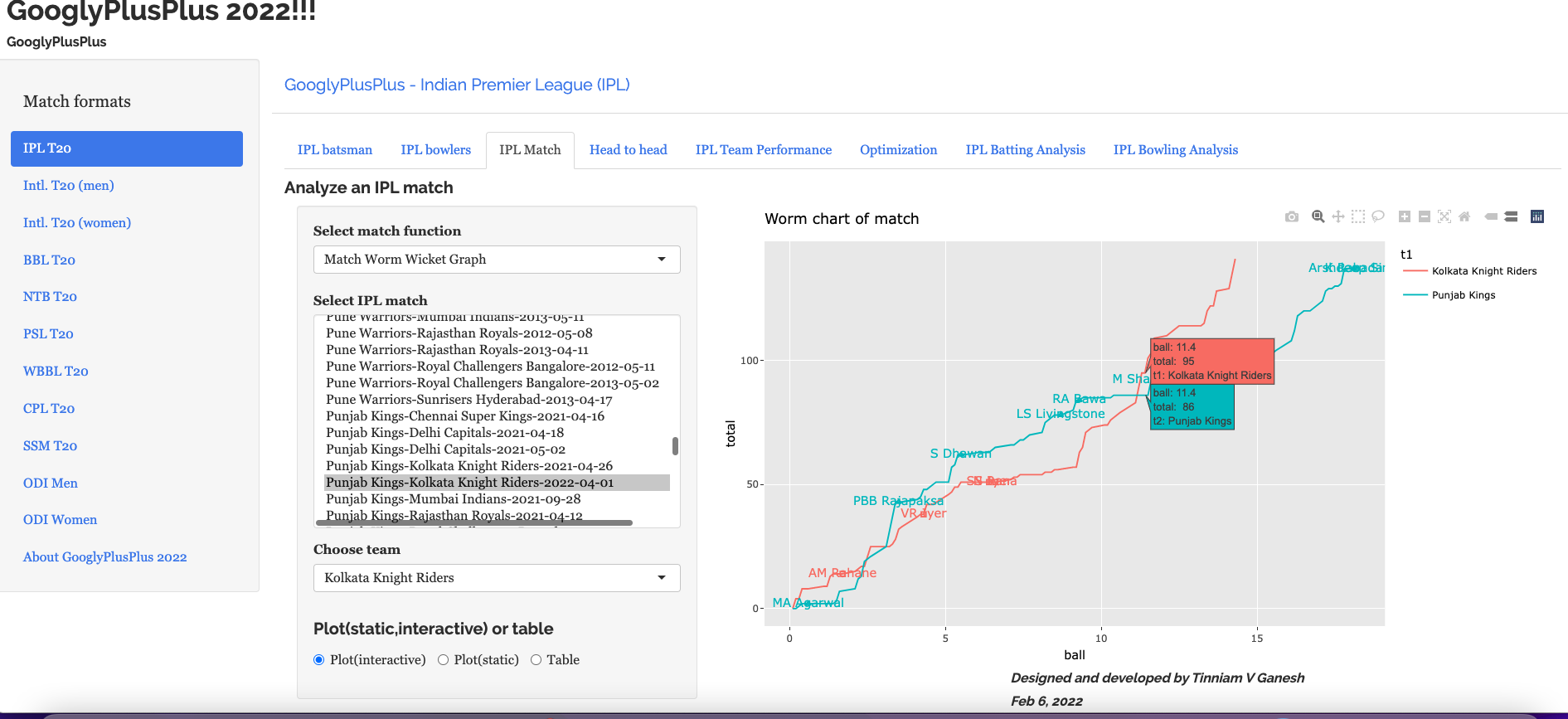
c) KKR vs PBKS -Match wicket worm chart – 1 Apr 2022
B) Batsmen tab
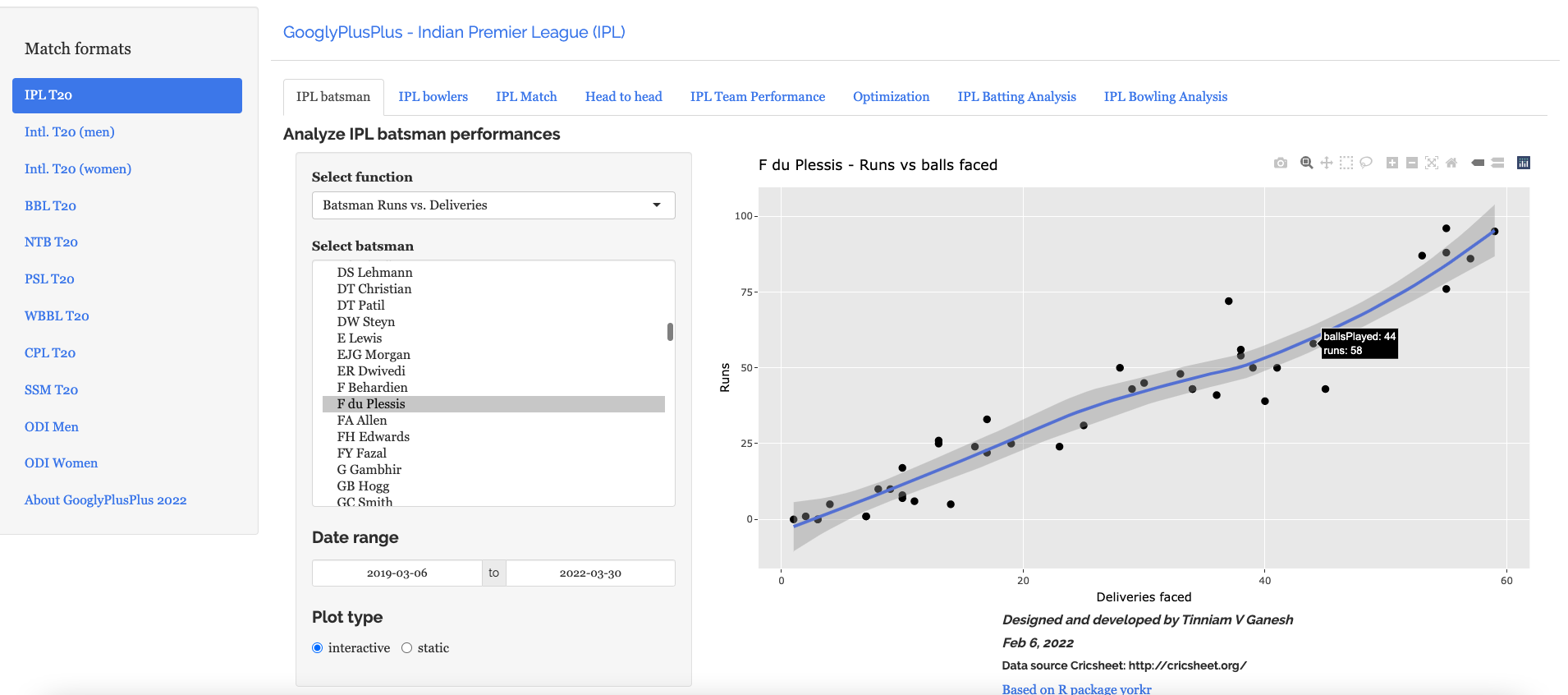
a) Faf Du Plessis – Runs vs Deliveries
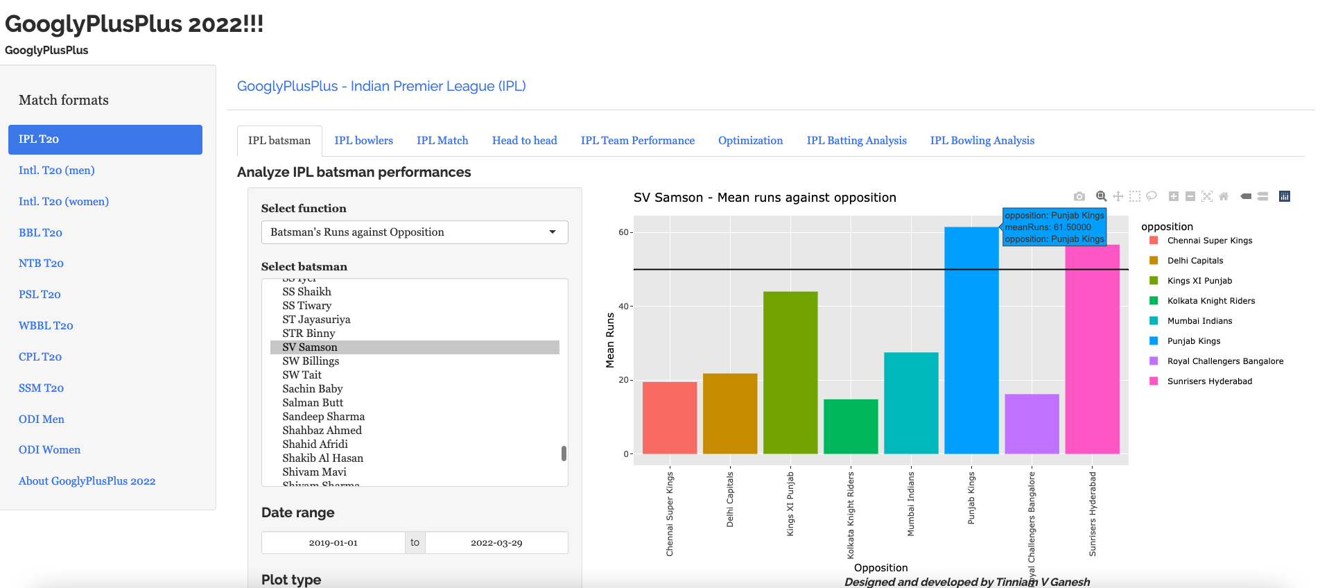
b) Sanju Samson – Runs against opposition
C) Bowler’s tab
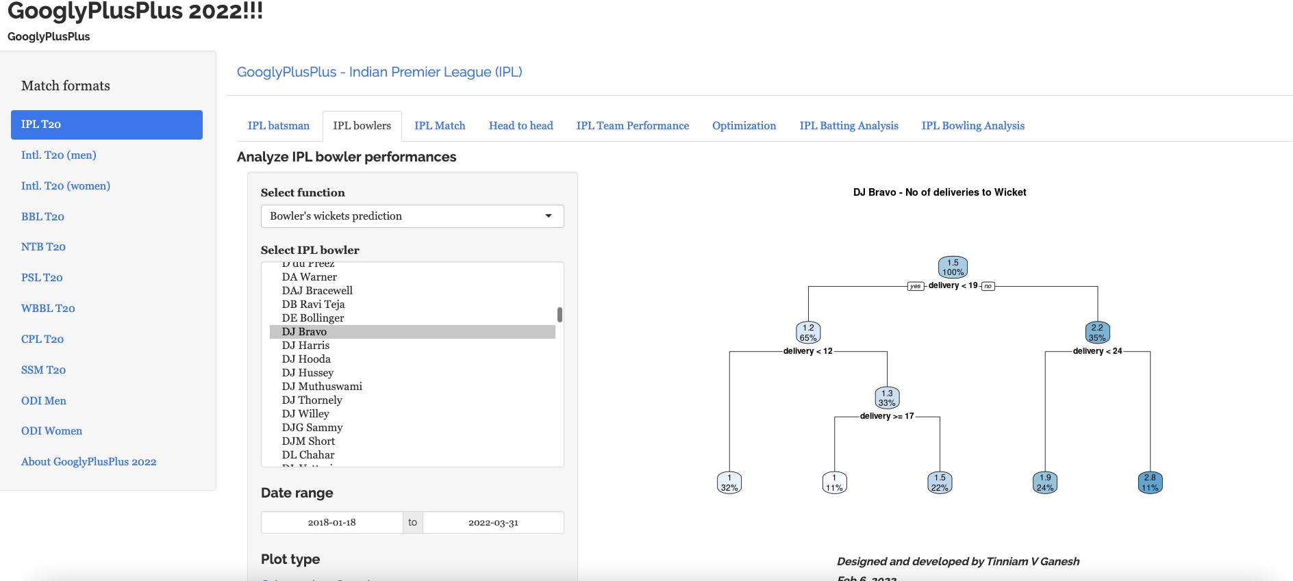
a) D J Bravo – No of deliveries to wicket
b) Trent Boult – Wickets at Venues
D) Head-to-head tab
a) DC vs MI – Mar -2019 till date : Batting scorecard
b) CSK vs KKR – Jan 2019 till date : Runs vs SR
E) Team vs All Teams tab
a) Punjab Kings vs all Teams – Wickets vs ER in Power play
b) Rajasthan Royals vs all Teams : Jan 2019 till date : Runs vs SR in Power play
F) Optimisation tab
a) Batsmen vs Bowlers
b) Bowlers vs batsmen
G) Batting analysis
This tab is for ranking batsmen
a) Batsmen rank from 2019 till date (Runs over SR)
Analytics for e.g. sports analytics, business analytics or analytics in e-commerce or in other domain has 2 main requirements namely a) What kind of analytics (set of parameters,function) will squeeze out the most intelligence from the data b) How to represent the analytics so that an expert can garner maximum insight?
While it may appear that the former is more important, the latter is also equally, if not, more vital to the problem. Indeed, a picture is worth a thousand words, and often times is more insightful than a large table of numbers. However, in the case of sports analytics, for e.g. in cricket a batting or bowling scorecard captures more information and can never be represented in chart.
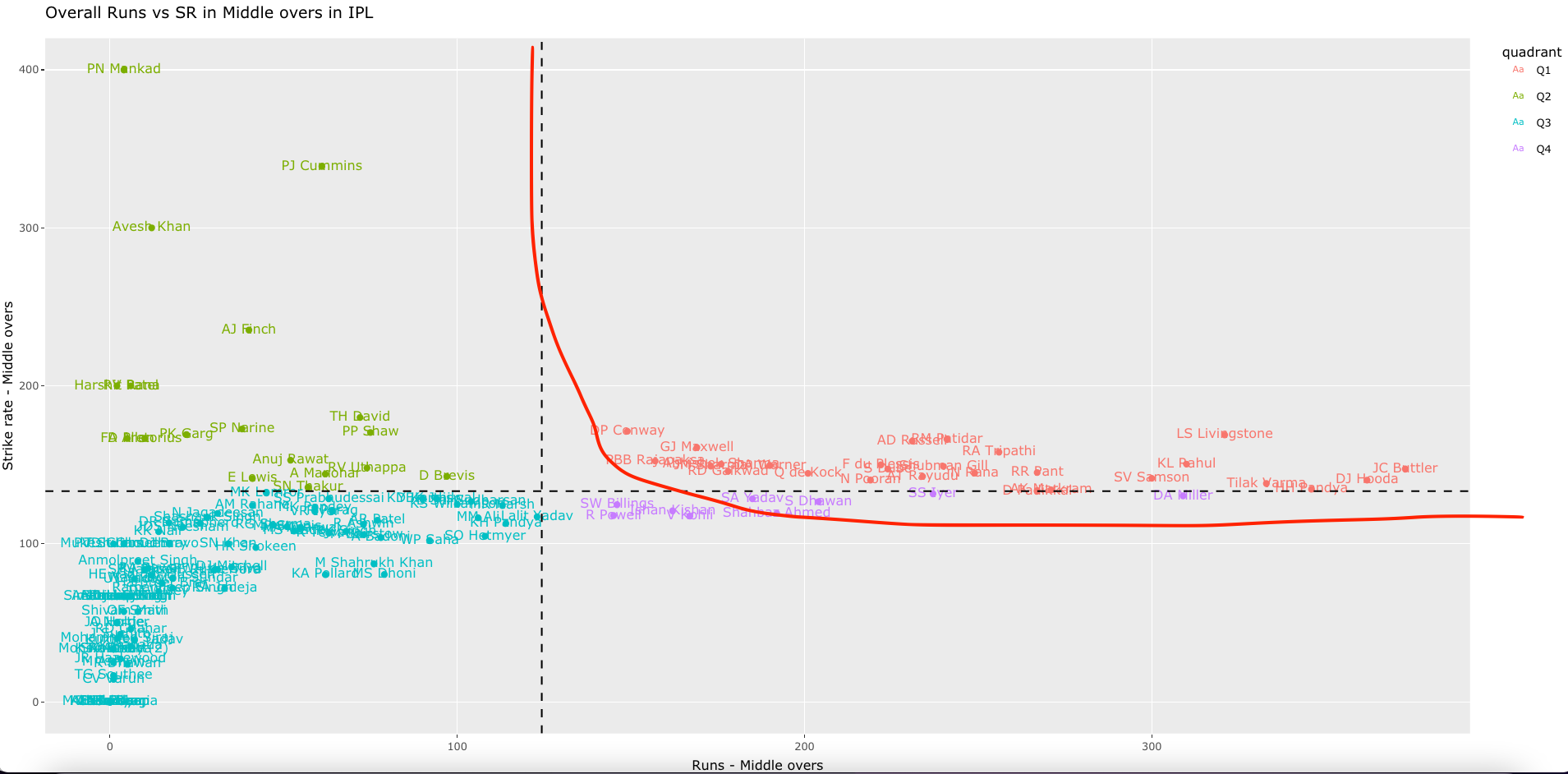
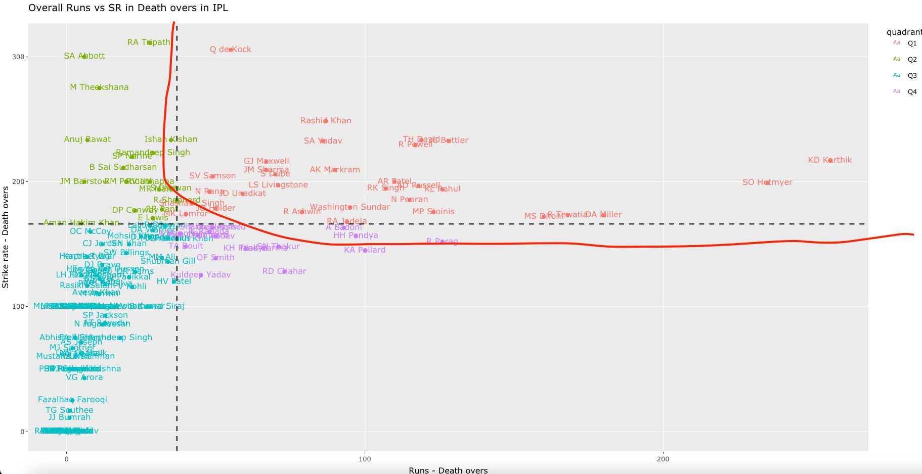
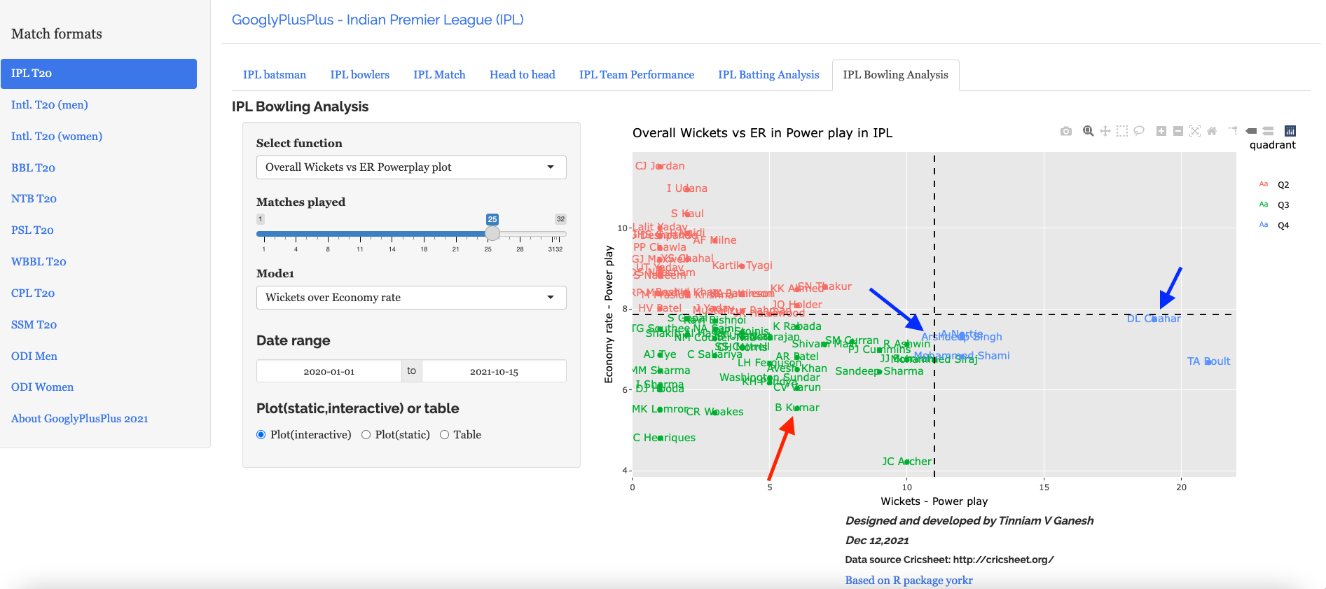
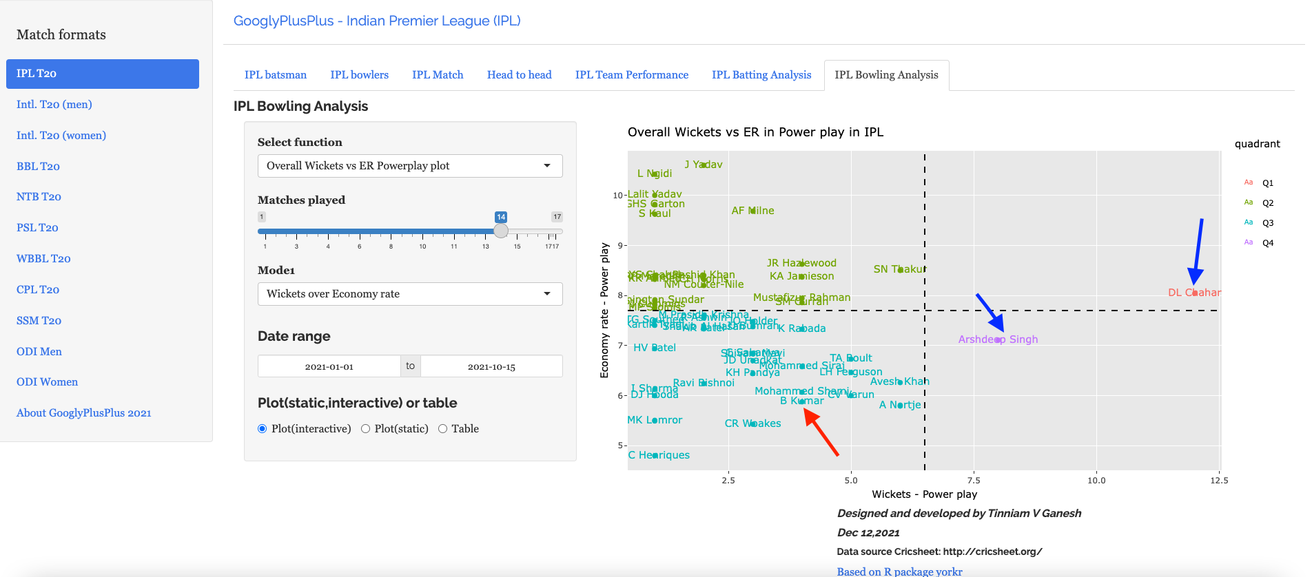
So, my Shiny app GooglyPlusPlus includes both charts and tables for different aspects of the analysis. In this post, a newer type of chart, popular among senior management experts, namely the 4 quadrant graph is introduced, which helps in categorising batsmen and bowlers into 4 categories as shown below
a) Batting Performances – Top right quadrant (High runs, High Strike rate)
b) Bowling Performances – Bottom right quadrant( High wickets, Low Economy Rate)
I have added the following 32 functions in this latest version of GooglyPlusPlus
A. Match Tab
All the functions below are at match level
Team Runs vs SR Plot
Team Wickets vs ER Plot
Team Runs vs SR Power play plot
Team Runs vs SR Middle overs plot
Team Runs vs SR Death overs plot
Team Wickets vs ER Power Play
Team Wickets vs ER Middle overs
Team Wickets vs ER Death overs
B. Head-to-head Tab
The below functions are based on all matches between 2 teams’
Team Runs vs SR Plot all Matches
Team Wickets vs ER Plot all Matches
Team Runs vs SR Power play plot all Matches
Team Runs vs SR Middle overs plot all Matches
Team Runs vs SR Death overs plot all Matches
Team Wickets vs ER Power Play plot all Matches
Team Wickets vs ER Middle overs plot all Matches
Team Wickets vs ER Death overs plot all Matches
C. Team Performance tab
The below functions are based on a team’s performance against all other teams
Team Runs vs SR Plot overall
Team Wickets vs ER Plot overall
Team Runs vs SR Power play plot overall
Team Runs vs SR Middle overs plot overall
Team Runs vs SR Death overs plot overall
Team Wickets vs ER Power Play overall
Team Wickets vs ER Middle overs overall
Team Wickets vs ER Death overs overall
D. T20 format Batting Analysis
This analysis is at T20 format level (IPL, Intl. T20(men), Intl. T20 (women), PSL, CPL etc.)
Overall Runs vs SR plot
Overall Runs vs SR Power play plot
Overall Runs vs SR Middle overs plot
Overall Runs vs SR Death overs plot
E. T20 Bowling Analysis
This analysis is at T20 format level (IPL, Intl. T20(men), Intl. T20 (women), PSL, CPL etc.)
Overall Wickets vs ER plot
Team Wickets vs ER Power Play
Team Wickets vs ER Middle overs
Team Wickets vs ER Death overs
These 32 functions have been added to my yorkr package and so all these functions become plug-n-play in my Shiny app GooglyPlusPlus2021 which means that the 32 functions apply across all the nine T20 formats that the app supports i.e. IPL, Intl. T20 (men), Intl. T20 (women), BBL, NTB, PSL, CPL, SSM, WBB.
Hence the multiplicative factor of the new addition is 32 x 9 = 288 additional ways of exploring match, team and player data
You can clone/fork GooglyPlusPlus from Github at gpp2021-10
Check out my app GooglyPlusPlus2021 and analyze batsmen, bowlers, teams, overall performance. The data for all the nine T20 formats have been updated to include the latest data.
Hence, the app is just in time for the IPL mega auction. You should be able to analyse players in IPL, Intl. T20 or in any of the other formats from where they could be drawn and check out their relative standings
I am including some random plots to demonstrate the newly minted functions
Note 1: All plots are interactive. The controls are on the top right. You can hover over data, zoom-in, zoom-out, compare data etc by choosing the appropriate control. To know more about how to use the interactive charts see GooglyPlusPlus2021 is now fully interactive!!!
New Zealand batting, except K Williamson, the rest did not fire as much
For Australia, Warner, Maxwell and Marsh played good knocks to wrest control
II) Head-to-head
a) Wickets vs ER during Power play of Mumbai Indians in all matches against Chennai Super Kings (IPL)
b) Karachi Kings Runs vs SR during middle overs against Multan Sultans (PSL)
c) Wickets vs ER during death overs of Barbados Tridents in all matches against Jamaica Tallawahs (CPL)
III) Teams overall batting performance
India’s best T20 performers in Power play since 2018 (Intl. T20)
e) Australia’s best performers in Death overs since Mar 2017 (Intl. T20)
f) India’s Intl. T20 (women) best Runs vs SR since 2018
g) England’s Intl. T20 (women) best bowlers in Death overs
IV) Overall Batting Performanceacross T20
This tab gives the batsmen’s rank and overall batting performance across the T20 format.
a) Why was Hardik Pandya chosen, and why this was in error?
Of course, it provides an insight into why Hardik Pandya was chosen in India’s World cup team despite poor performances recently. Here are the best Intl. T20 death over batsmen
Of course, we can zoom in to get a better look
This is further substantiated when we performances in IPL
However, if you move the needle forward a year at a time, you see Hardik Pandya’s performance drops significantly
and further down
Rather, Dinesh Karthik, Sanju Samson or Ruturaj Gaikwad would have been better options
b) Best batsmen Intl. T20 (women) in Power play since 2018
V) Overall bowling performance
This tab gives the bowler’s rank and overall bowling performance in Power play, middle and death overs across all T20 formats
a) Intl. T20 (men) best bowlers in Power Play from 2019 (zoomed in)
b) Intl. T20(men) best bowlers in Death overs since 2019
c) Was B. Kumar a good choice for India team in World cup?
Bhuvi was one of India’s best bowler in Power play only if we go back to the beginning of time
i) From 2008
But if we move forward to 2020 onwards we see Arshdeep Singh or D Chahar would have been a better choice
ii) From 2020 onwards
iii) 2021 onwards
Hence D Chahar & Arshdeep Singh are the natural choice moving forwards for India
iv) T20 Best batsman
If we look at Intl. T20 performances since 2017, Babar Azam leads the pack, however his Strike rate needs to move up.
This latest edition of GooglyPlusPlus2021 now includes detailed analysis of teams, batsmen and bowlers in power play, middle and death overs. The T20 format is based on 3 phases as each side faces 20 overs.
Power play: Overs: 0 – 6 – No more than 2 players can be outside the 30 yard circle
Middle overs: Overs: 7- 16 – During these overs the batting side tries to consolidate their innings
Death overs: Overs: 16 -20 – During these 5 overs the batting side tries to accelerate the scoring rate, while the bowling side will try to restrict the batsmen against going for big hits
This is shown below
This latest update of GooglyPlusPlus2021 includes the following functions
a) Match tab
teamRunsAcrossOvers
teamSRAcrossOvers
teamWicketsAcrossOvers
teamERAcrossOvers
matchWormWickets
b) Head-to-head tab
teamRunsAcrossOversOppnAllMatches
teamSRAcrossOversOppnAllMatches
teamWicketsAcrossOversOppnAllMatches
teamERAcrossOversOppnAllMatches
topRunsBatsmenAcrossOversOppnAllMatches
topSRBatsmenAcrossOversOppnAllMatches
topWicketsBowlersAcrossOversOppnAllMatches
topERBowlerAcrossOverOppnAllMatches
c) Overall performance tab
teamRunsAcrossOversAllOppnAllMatches
teamSRAcrossOversAllOppnAllMatches
teamWicketsAcrossOversAllOppnAllMatches
teamERAcrossOversAllOppnAllMatches
topRunsBatsmenAcrossOversAllOppnAllMatches
topSRBatsmenAcrossOversAllOppnAllMatches
topWicketsBowlersAcrossOversAllOppnAllMatches
topERBowlerAcrossOverAllOppnAllMatches
Hence a total of 8 + 8 + 5 = 21 functions have been added. These functions can be utilized across all the 9 T20 formats that are supported in GooglyPlusPlus2021 namely
You can clone/fork the code for the Shiny app from Github – gpp2021-9
Included below is a random selection of options from the 189 possibilities mentioned above. Feel free to try out for yourself
A) IPL – CSK vs KKR 2018-04-10
a) Team Runs in power play, middle and death overs
b) Team Strike rate in power play, middle and death overs
B) Intl. T20 (men) – India vs Afghanistan (2021-11-03)
a) Team wickets in power play, middle and death overs
b) Team Economy rate in power play, middle and death overs
C) Intl. T20 (women) Head-to-head : India vs Australia since 2018
a) Team Runs in all matches in power play, middle and death overs
D) PSL Head-to-head strike rate since 2019
a) Team vs team Strike rate : Karachi Kings vs Lahore Qalanders since 2019 in power play, middle and death overs
E) Team overall performance in all matches against all opposition
a) BBL : Brisbane Heats : Team Wickets between 2015 – 2018 in power play, middle and death overs
F) Top Runs and Strike rate Batsman of Mumbai Indians vs Royal Challengers Bangalore since 2018
a) Top runs scorers for Mumbai Indians (MI) in power play, middle and death overs
b) Top strike rate for RCB in power play, middle and death overs
F) Intl. T20 (women) India vs England since 2018
a) Top wicket takers for England in power play, middle and death overs since 2018
b) Top wicket takers for India in power play, middle and death overs since 2018
G) Intl. T20 (men) All time best batsmen and bowlers for India
a) Most runs in power play, middle and death overs
b) Highest strike rate in power play, middle and death overs
H) Match worm wicket chart
In addition to the usual Match worm chart, I have also added a Match Wicket worm chart in the latest version
Note: You can zoom to the area where you would like to focus more
The option of looking at the Match worm chart (without wickets) also exists.
Go ahead take GooglyPlusPlus2021 for a test drive and check out how your favourite players perform in power play, middle and death overs. Click GooglyPlusPlus2021
You can fork/download the app code from Github at gpp2021-9