Introduction
In this post my package ‘cricketr’ takes a swing at One Day Internationals(ODIs). Like test batsman who adapt to ODIs with some innovative strokes, the cricketr package has some additional functions and some modified functions to handle the high strike and economy rates in ODIs. As before I have chosen my top 4 ODI batsmen and top 4 ODI bowlers.

If you are passionate about cricket, and love analyzing cricket performances, then check out my racy book on cricket ‘Cricket analytics with cricketr and cricpy – Analytics harmony with R & Python’! This book discusses and shows how to use my R package ‘cricketr’ and my Python package ‘cricpy’ to analyze batsmen and bowlers in all formats of the game (Test, ODI and T20). The paperback is available on Amazon at $21.99 and the kindle version at $9.99/Rs 449/-. A must read for any cricket lover! Check it out!!
You can download the latest PDF version of the book at ‘Cricket analytics with cricketr and cricpy: Analytics harmony with R and Python-6th edition‘

Important note 1: The latest release of ‘cricketr’ now includes the ability to analyze performances of teams now!! See Cricketr adds team analytics to its repertoire!!!
Important note 2 : Cricketr can now do a more fine-grained analysis of players, see Cricketr learns new tricks : Performs fine-grained analysis of players
Important note 3: Do check out the python avatar of cricketr, ‘cricpy’ in my post ‘Introducing cricpy:A python package to analyze performances of cricketers”
Do check out my interactive Shiny app implementation using the cricketr package – Sixer – R package cricketr’s new Shiny avatar
You can also read this post at Rpubs as odi-cricketr. Dowload this report as a PDF file from odi-cricketr.pdf
Important note: Do check out my other posts using cricketr at cricketr-posts
Note: If you would like to do a similar analysis for a different set of batsman and bowlers, you can clone/download my skeleton cricketr template from Github (which is the R Markdown file I have used for the analysis below). You will only need to make appropriate changes for the players you are interested in. Just a familiarity with R and R Markdown only is needed.
Batsmen
- Virendar Sehwag (Ind)
- AB Devilliers (SA)
- Chris Gayle (WI)
- Glenn Maxwell (Aus)
Bowlers
- Mitchell Johnson (Aus)
- Lasith Malinga (SL)
- Dale Steyn (SA)
- Tim Southee (NZ)
I have sprinkled the plots with a few of my comments. Feel free to draw your conclusions! The analysis is included below
The profile for Virender Sehwag is 35263. This can be used to get the ODI data for Sehwag. For a batsman the type should be “batting” and for a bowler the type should be “bowling” and the function is getPlayerDataOD()
The package can be installed directly from CRAN
if (!require("cricketr")){
    install.packages("cricketr",lib = "c:/test")
}
library(cricketr)
or from Github
library(devtools)
install_github("tvganesh/cricketr")
library(cricketr)
The One day data for a particular player can be obtained with the getPlayerDataOD() function. To do you will need to go to ESPN CricInfo Player and type in the name of the player for e.g Virendar Sehwag, etc. This will bring up a page which have the profile number for the player e.g. for Virendar Sehwag this would be http://www.espncricinfo.com/india/content/player/35263.html. Hence, Sehwag’s profile is 35263. This can be used to get the data for Virat Sehwag as shown below
sehwag <- getPlayerDataOD(35263,dir="..",file="sehwag.csv",type="batting")
Analyses of Batsmen
The following plots gives the analysis of the 4 ODI batsmen
- Virendar Sehwag (Ind) – Innings – 245, Runs = 8586, Average=35.05, Strike Rate= 104.33
- AB Devilliers (SA) – Innings – 179, Runs= 7941, Average=53.65, Strike Rate= 99.12
- Chris Gayle (WI) – Innings – 264, Runs= 9221, Average=37.65, Strike Rate= 85.11
- Glenn Maxwell (Aus) – Innings – 45, Runs= 1367, Average=35.02, Strike Rate= 126.69
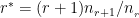
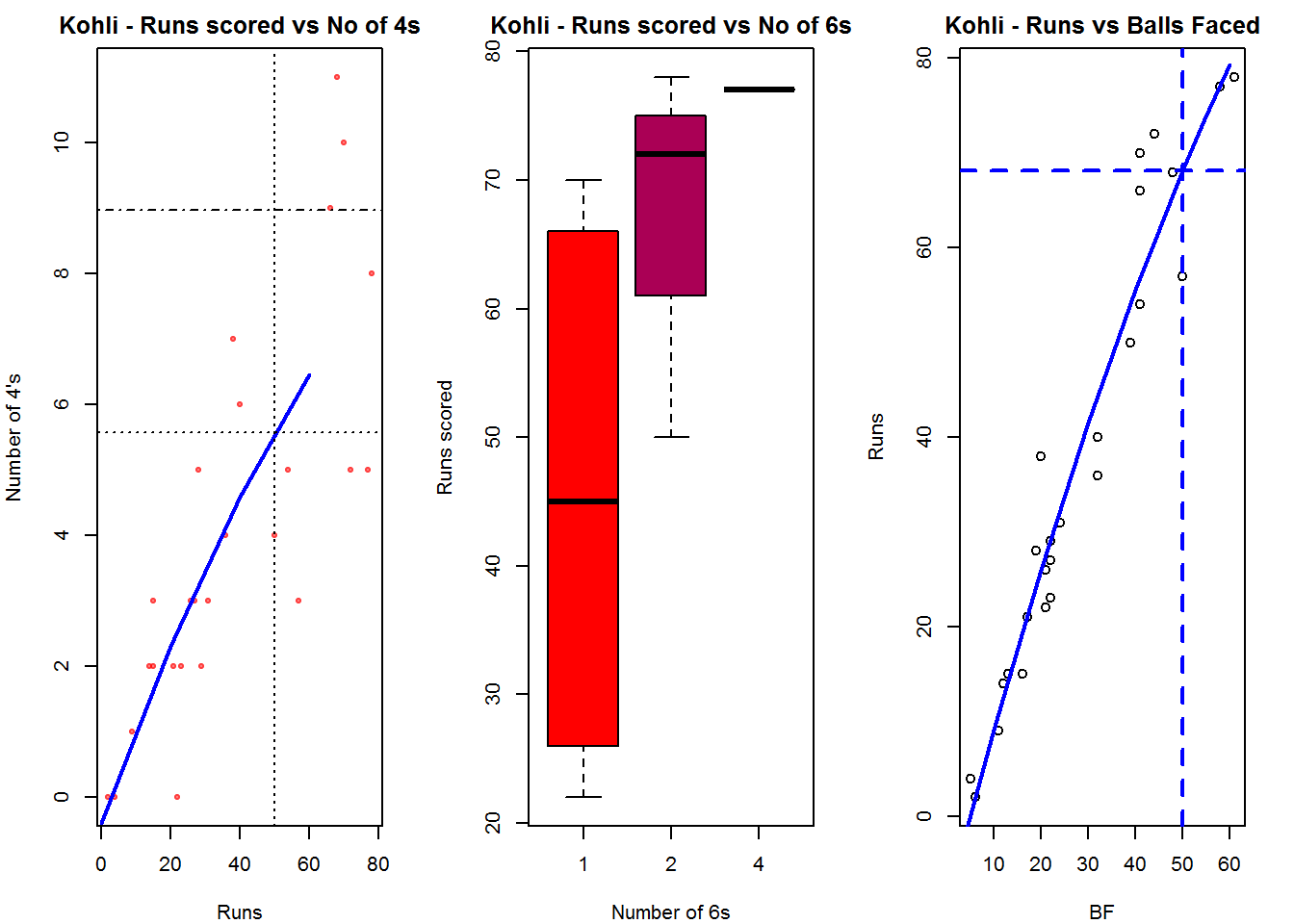
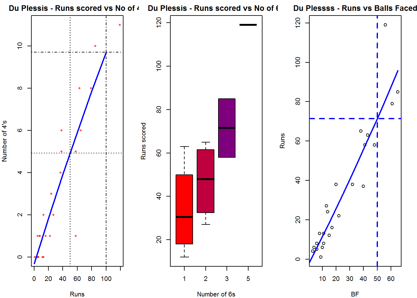
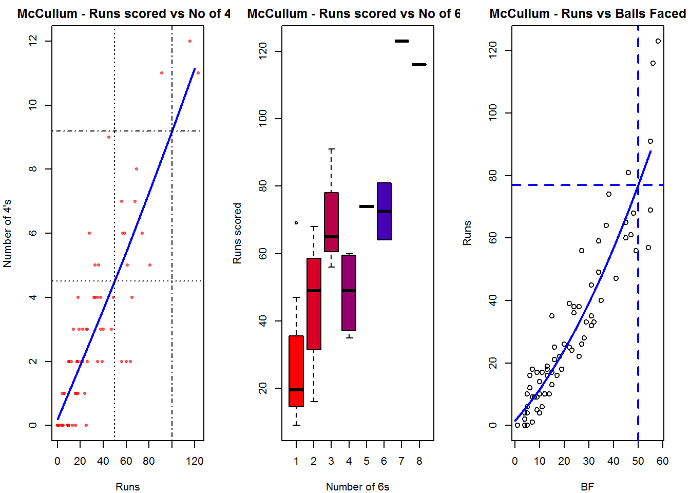
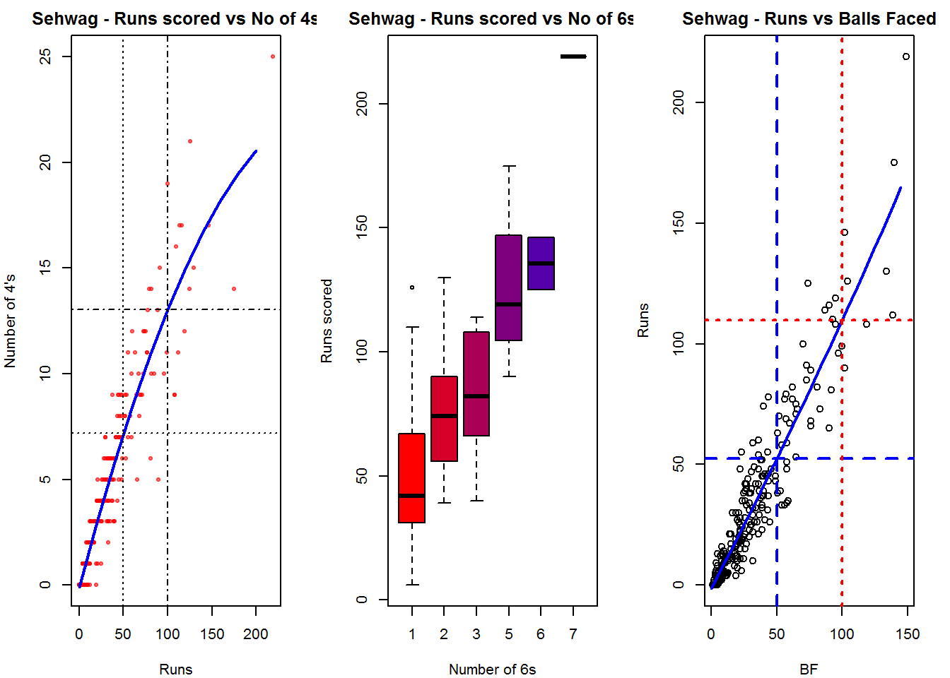
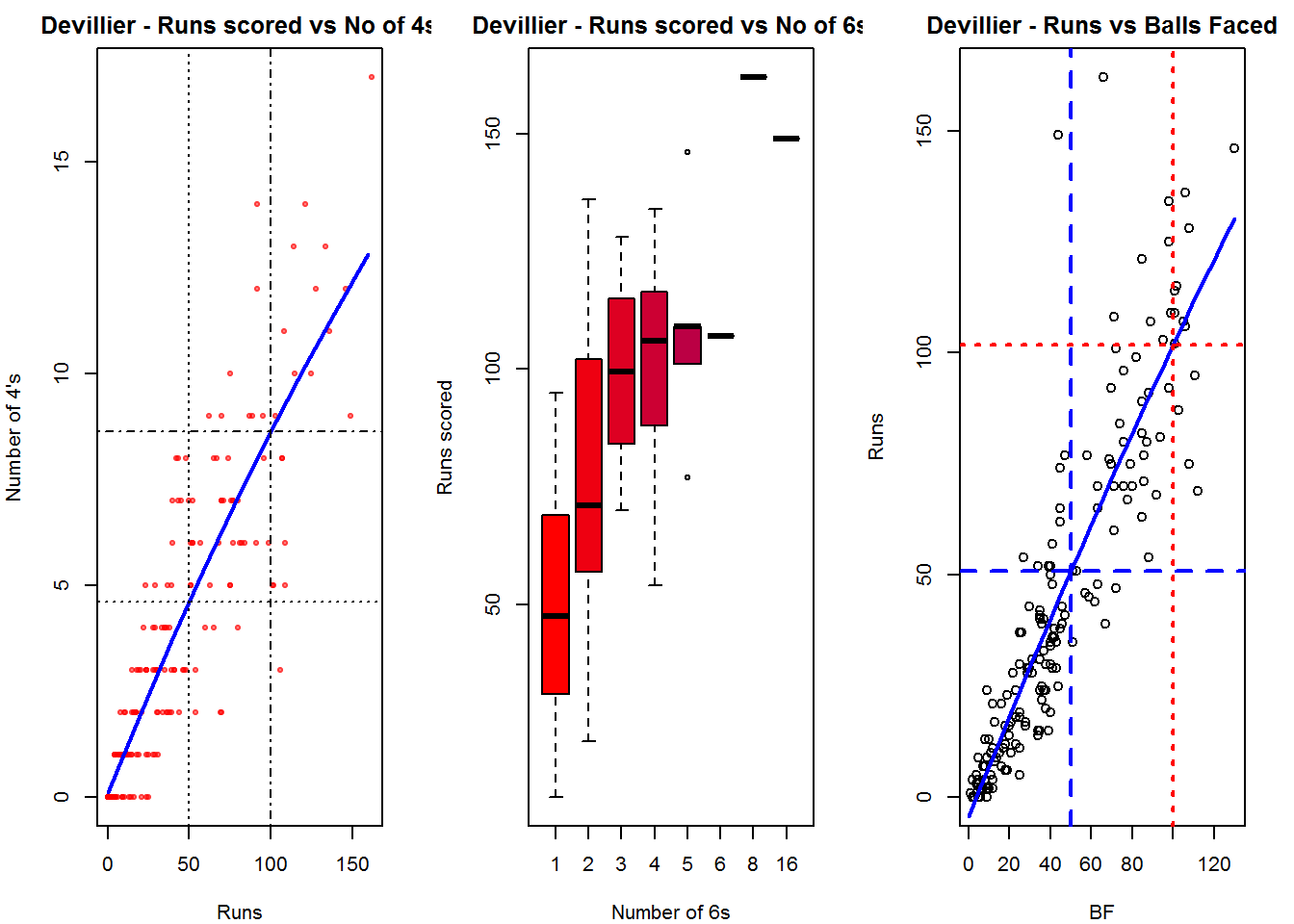
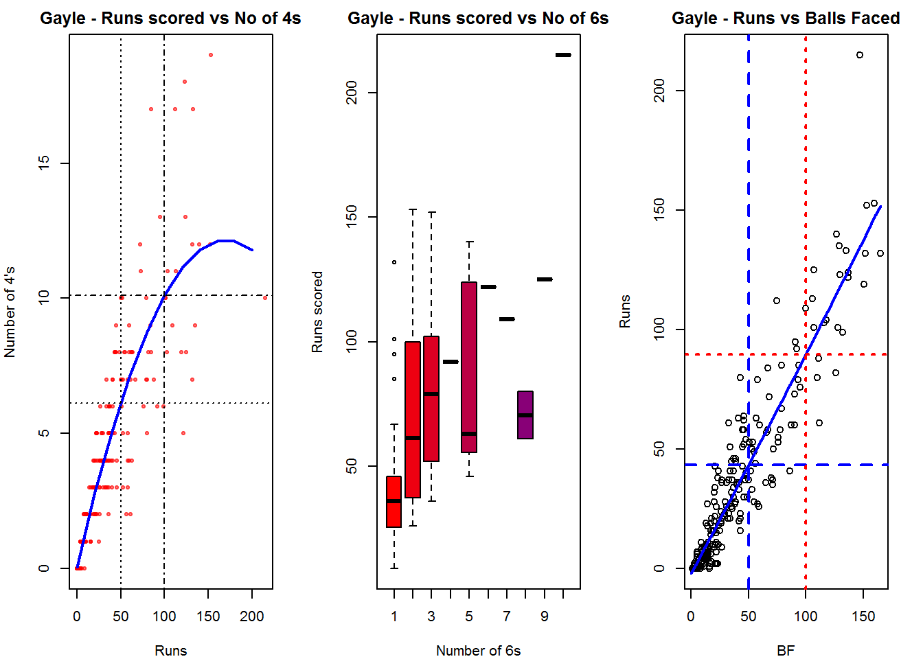
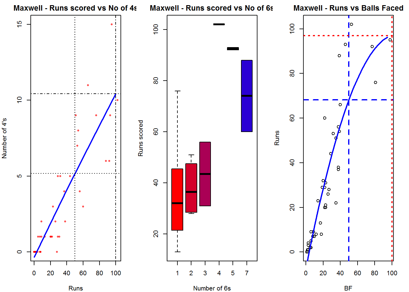
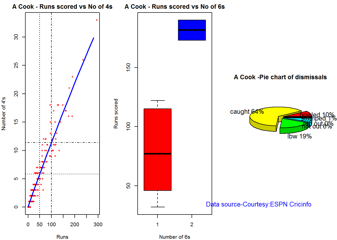
Plot of 4s, 6s and the scoring rate in ODIs
The 3 charts below give the number of
- 4s vs Runs scored
- 6s vs Runs scored
- Balls faced vs Runs scored
A regression line is fitted in each of these plots for each of the ODI batsmen A. Virender Sehwag
par(mfrow=c(1,3))
par(mar=c(4,4,2,2))
batsman4s("./sehwag.csv","Sehwag")
batsman6s("./sehwag.csv","Sehwag")
batsmanScoringRateODTT("./sehwag.csv","Sehwag")

dev.off()
## null device
##           1
B. AB Devilliers
par(mfrow=c(1,3))
par(mar=c(4,4,2,2))
batsman4s("./devilliers.csv","Devillier")
batsman6s("./devilliers.csv","Devillier")
batsmanScoringRateODTT("./devilliers.csv","Devillier")

dev.off()
## null device
##           1
C. Chris Gayle
par(mfrow=c(1,3))
par(mar=c(4,4,2,2))
batsman4s("./gayle.csv","Gayle")
batsman6s("./gayle.csv","Gayle")
batsmanScoringRateODTT("./gayle.csv","Gayle")

dev.off()
## null device
##           1
D. Glenn Maxwell
par(mfrow=c(1,3))
par(mar=c(4,4,2,2))
batsman4s("./maxwell.csv","Maxwell")
batsman6s("./maxwell.csv","Maxwell")
batsmanScoringRateODTT("./maxwell.csv","Maxwell")

dev.off()
## null device
##           1
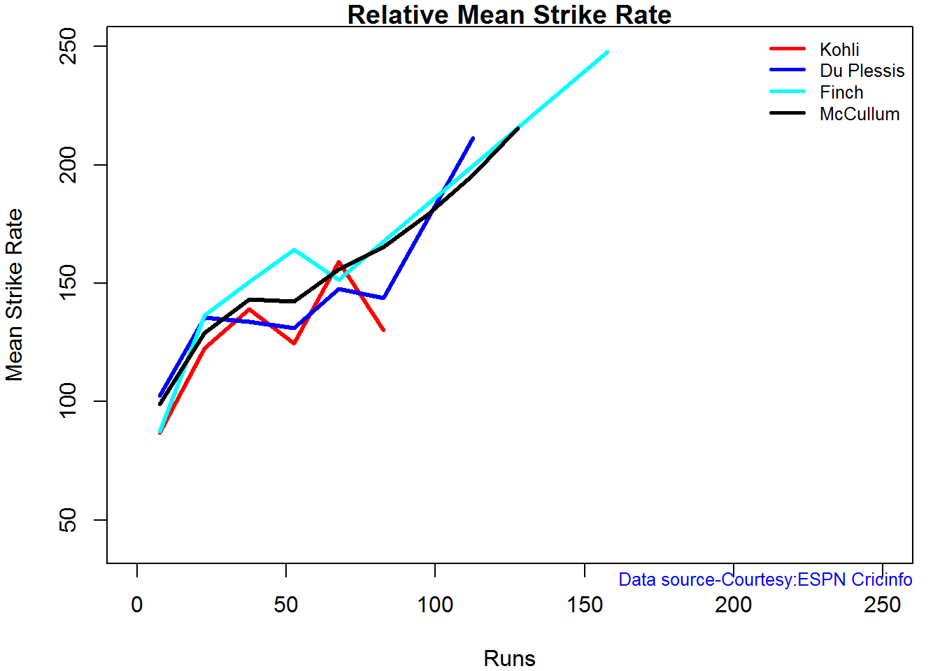
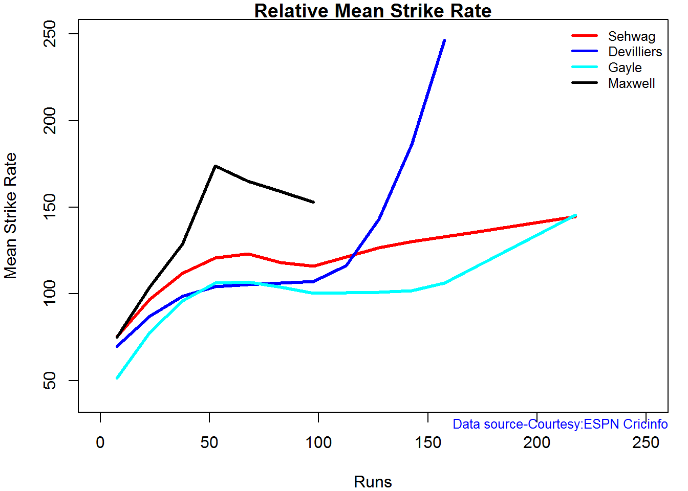
Relative Mean Strike Rate
In this first plot I plot the Mean Strike Rate of the batsmen. It can be seen that Maxwell has a awesome strike rate in ODIs. However we need to keep in mind that Maxwell has relatively much fewer (only 45 innings) innings. He is followed by Sehwag who(most innings- 245) also has an excellent strike rate till 100 runs and then we have Devilliers who roars ahead. This is also seen in the overall strike rate in above
par(mar=c(4,4,2,2))
frames <- list("./sehwag.csv","./devilliers.csv","gayle.csv","maxwell.csv")
names <- list("Sehwag","Devilliers","Gayle","Maxwell")
relativeBatsmanSRODTT(frames,names)

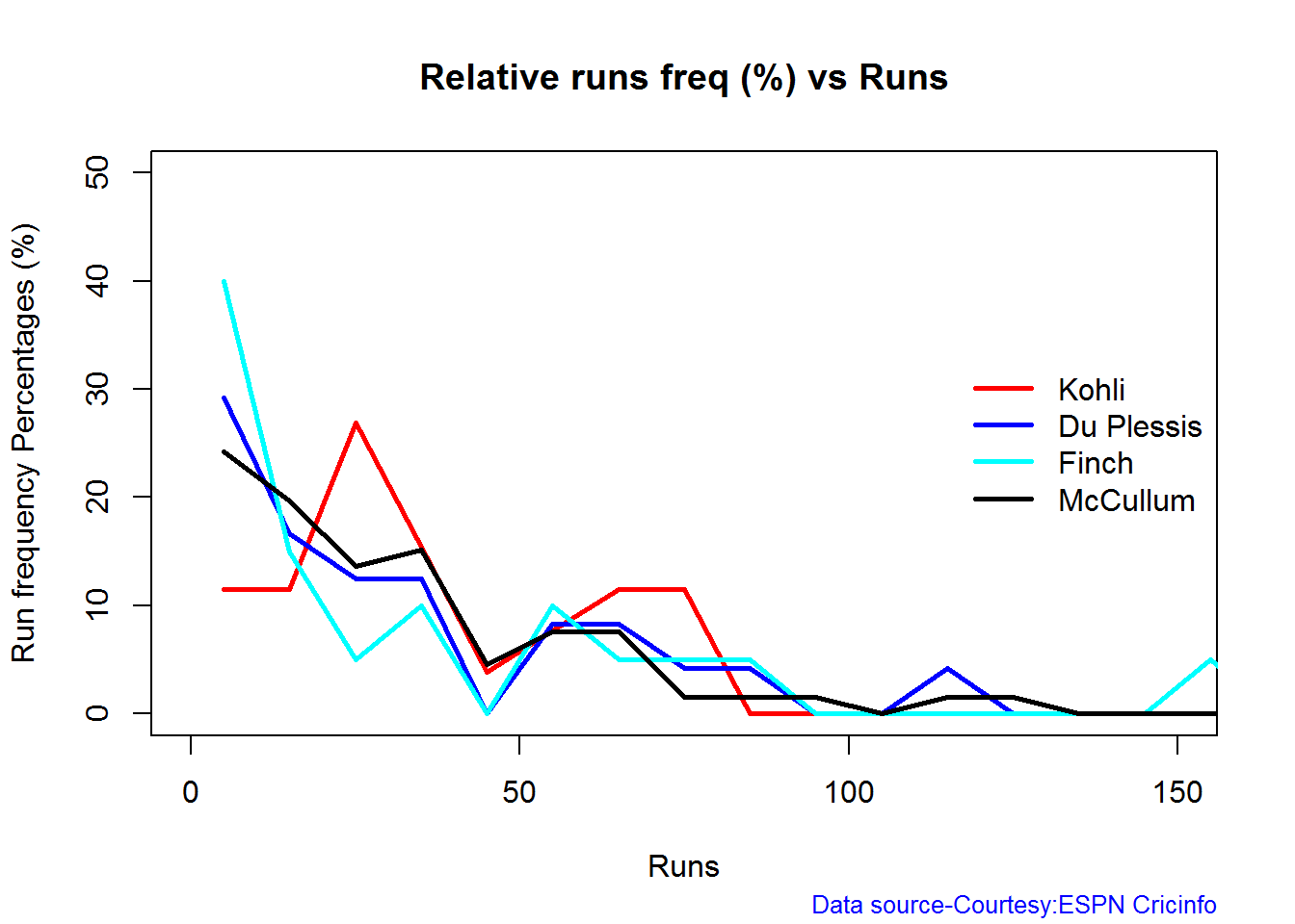
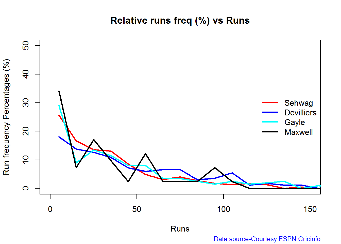
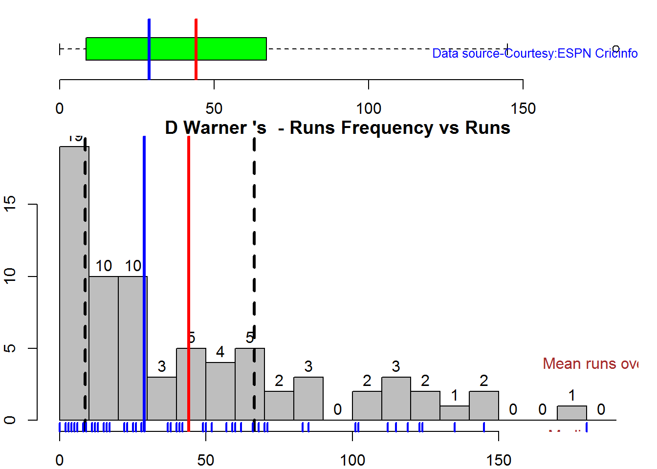
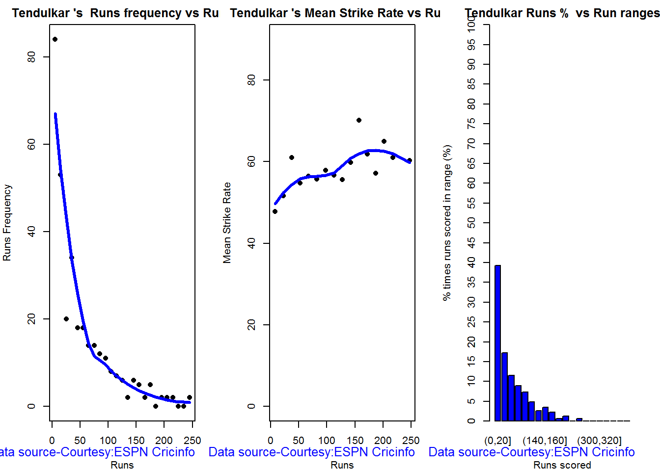
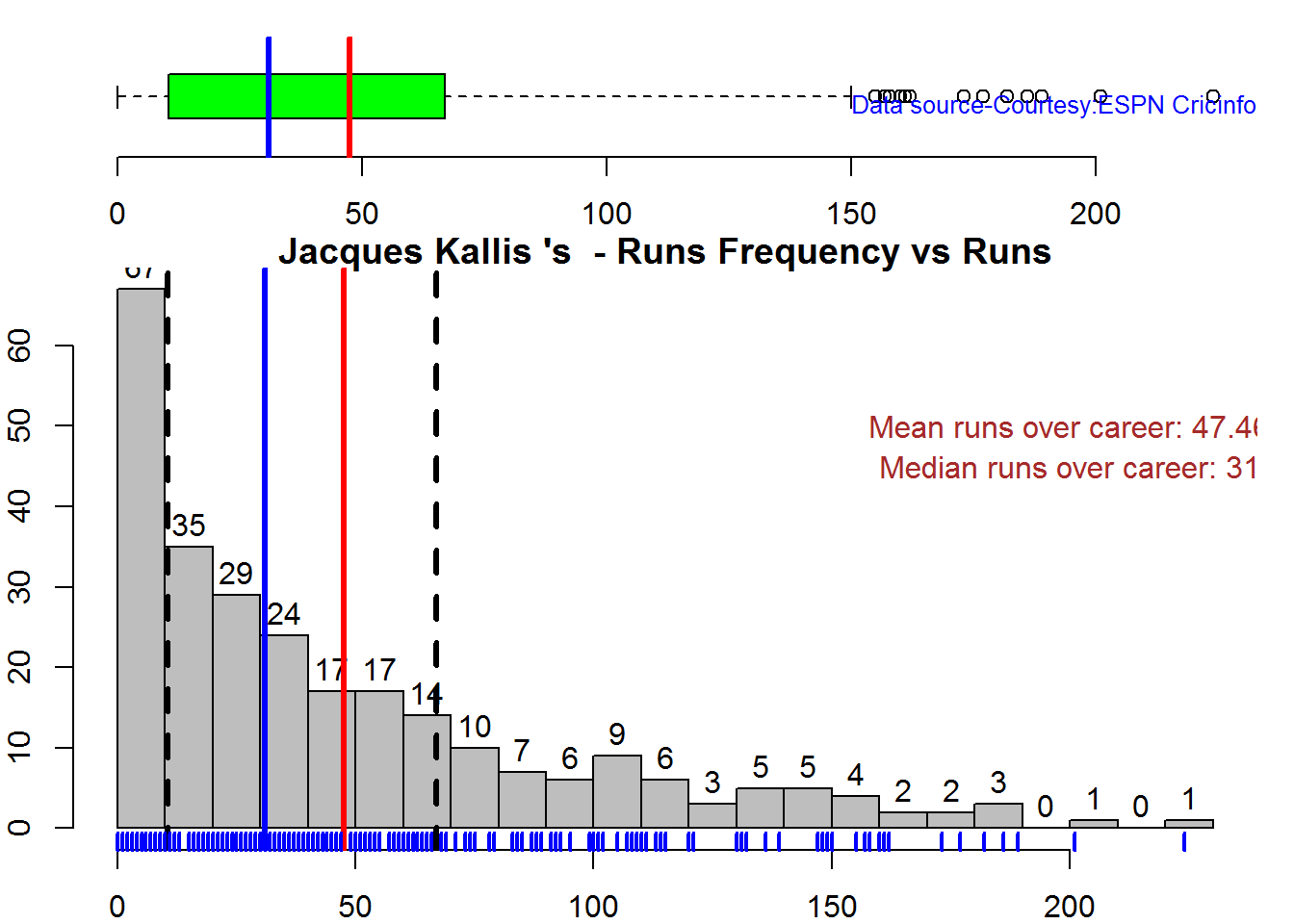
Relative Runs Frequency Percentage
Sehwag leads in the percentage of runs in 10 run ranges upto 50 runs. Maxwell and Devilliers lead in 55-66 & 66-85 respectively.
frames <- list("./sehwag.csv","./devilliers.csv","gayle.csv","maxwell.csv")
names <- list("Sehwag","Devilliers","Gayle","Maxwell")
relativeRunsFreqPerfODTT(frames,names)

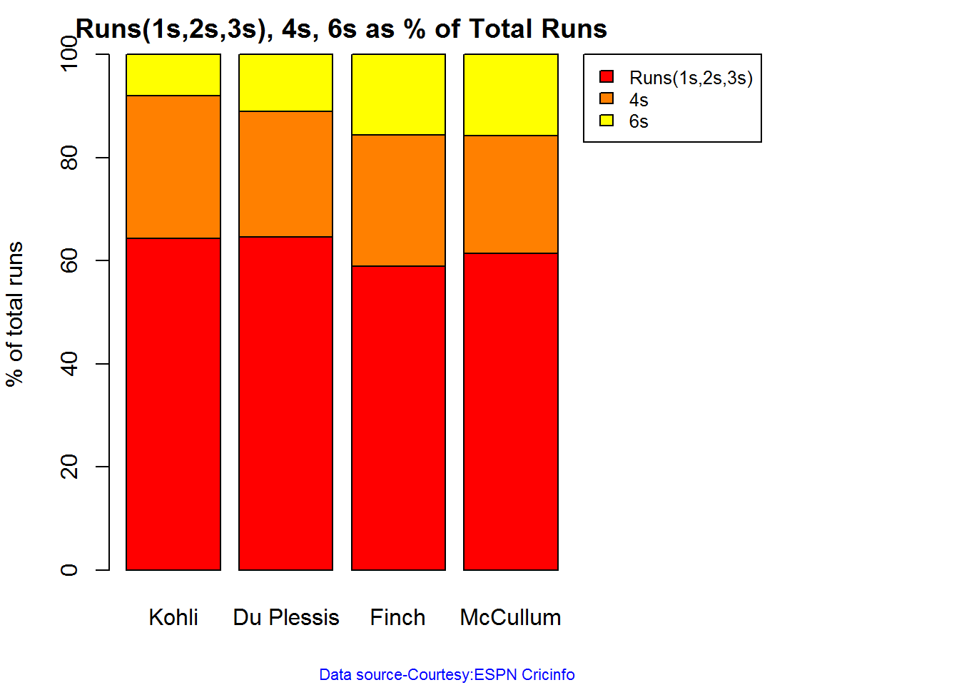
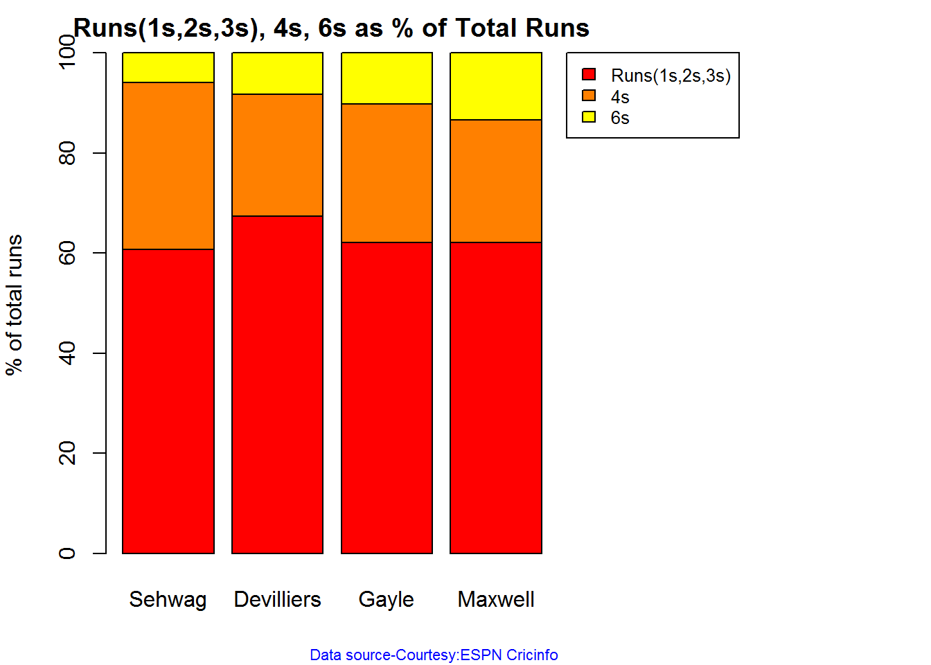
Percentage of 4s,6s in the runs scored
The plot below shows the percentage of runs made by the batsmen by ways of 1s,2s,3s, 4s and 6s. It can be seen that Sehwag has the higheest percent of 4s (33.36%) in his overall runs in ODIs. Maxwell has the highest percentage of 6s (13.36%) in his ODI career. If we take the overall 4s+6s then Sehwag leads with (33.36 +5.95 = 39.31%),followed by Gayle (27.80+10.15=37.95%)
Percent 4’s,6’s in total runs scored
The plot below shows the contrib
frames <- list("./sehwag.csv","./devilliers.csv","gayle.csv","maxwell.csv")
names <- list("Sehwag","Devilliers","Gayle","Maxwell")
runs4s6s <-batsman4s6s(frames,names)

print(runs4s6s)
## Sehwag Devilliers Gayle Maxwell
## Runs(1s,2s,3s) 60.69 67.39 62.05 62.11
## 4s 33.36 24.28 27.80 24.53
## 6s 5.95 8.32 10.15 13.36
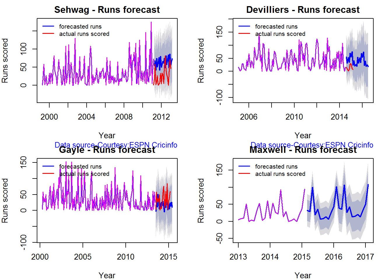
Runs forecast
The forecast for the batsman is shown below.
par(mfrow=c(2,2))
par(mar=c(4,4,2,2))
batsmanPerfForecast("./sehwag.csv","Sehwag")
batsmanPerfForecast("./devilliers.csv","Devilliers")
batsmanPerfForecast("./gayle.csv","Gayle")
batsmanPerfForecast("./maxwell.csv","Maxwell")

dev.off()
## null device
##           1
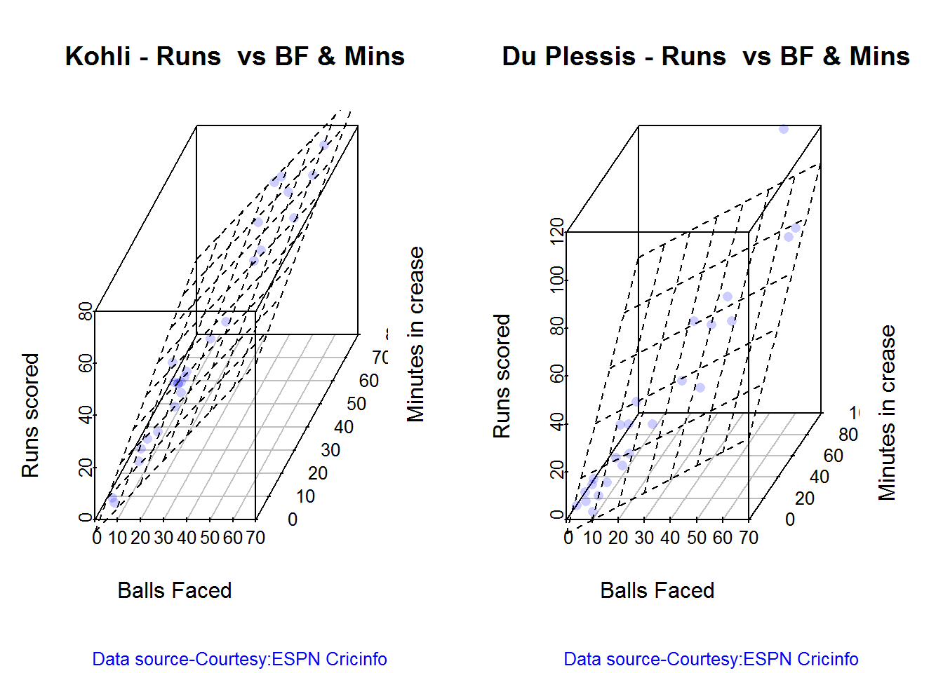
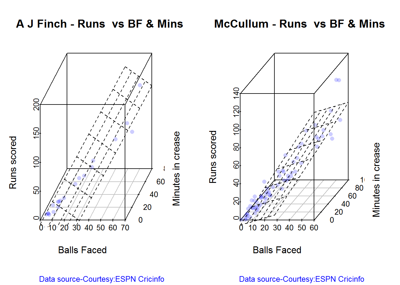
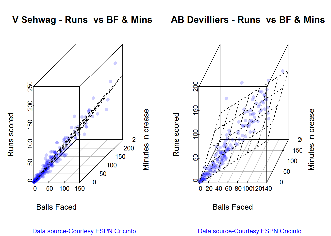
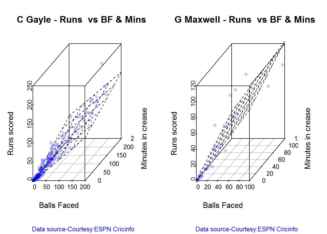
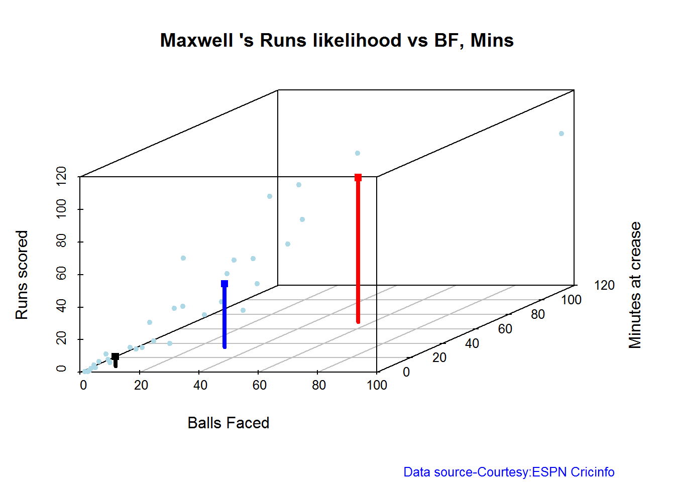
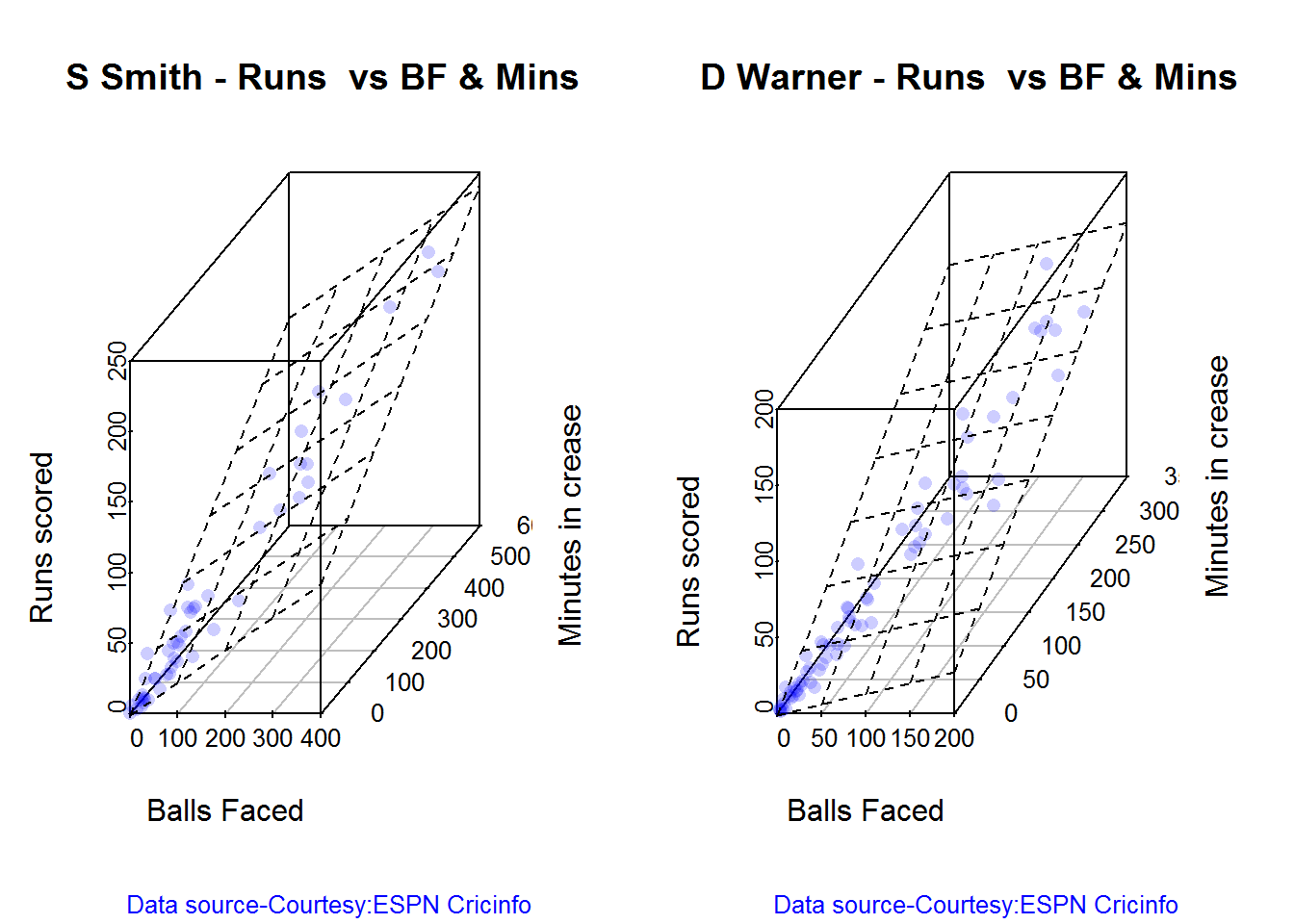
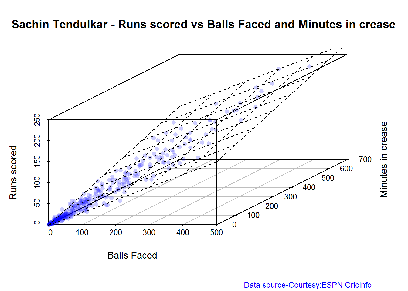
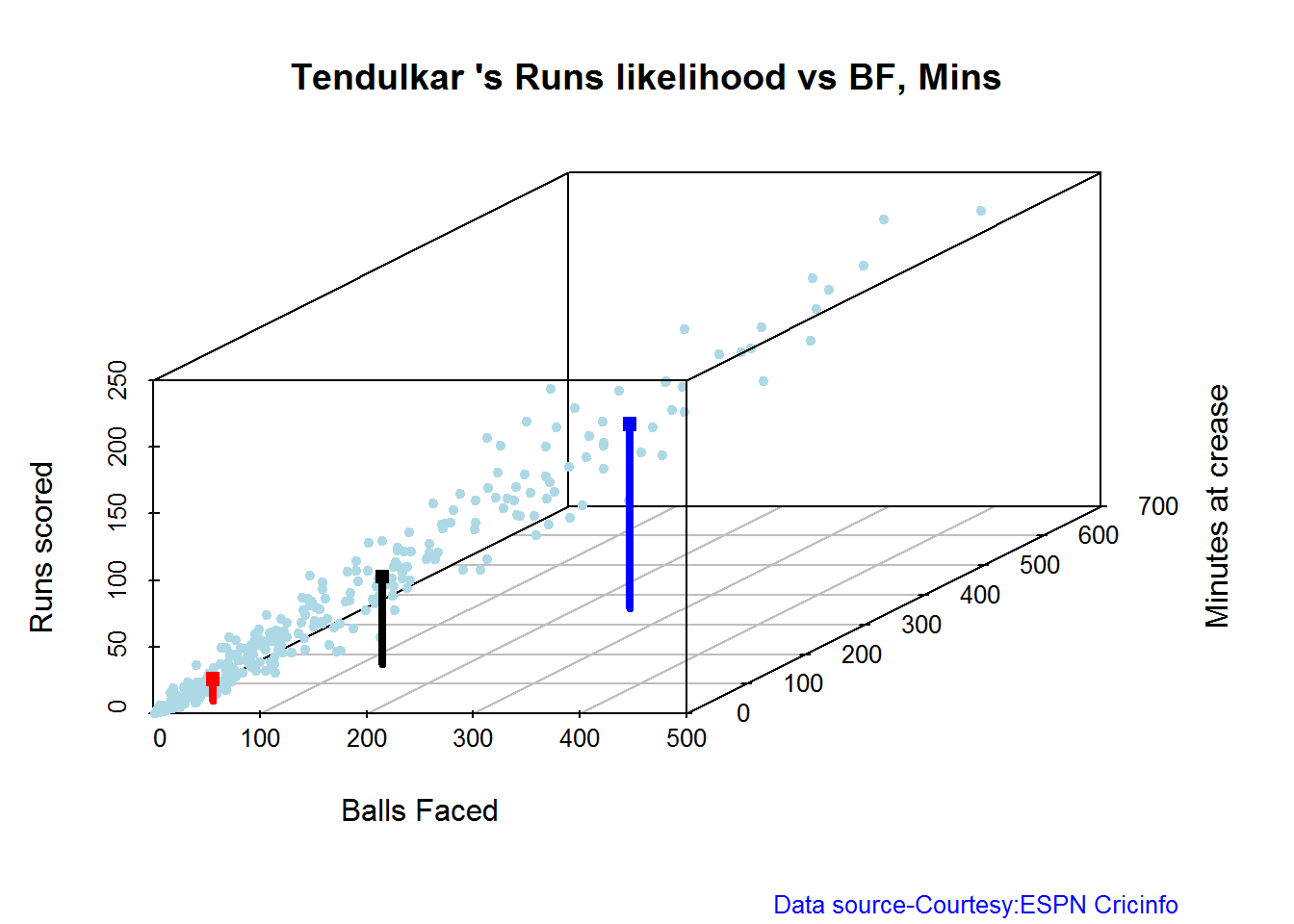
3D plot of Runs vs Balls Faced and Minutes at Crease
The plot is a scatter plot of Runs vs Balls faced and Minutes at Crease. A prediction plane is fitted
par(mfrow=c(1,2))
par(mar=c(4,4,2,2))
battingPerf3d("./sehwag.csv","V Sehwag")
battingPerf3d("./devilliers.csv","AB Devilliers")

dev.off()
## null device
##           1
par(mfrow=c(1,2))
par(mar=c(4,4,2,2))
battingPerf3d("./gayle.csv","C Gayle")
battingPerf3d("./maxwell.csv","G Maxwell")

dev.off()
## null device
##           1
Predicting Runs given Balls Faced and Minutes at Crease
A multi-variate regression plane is fitted between Runs and Balls faced +Minutes at crease.
BF <- seq( 10, 200,length=10)
Mins <- seq(30,220,length=10)
newDF <- data.frame(BF,Mins)
sehwag <- batsmanRunsPredict("./sehwag.csv","Sehwag",newdataframe=newDF)
devilliers <- batsmanRunsPredict("./devilliers.csv","Devilliers",newdataframe=newDF)
gayle <- batsmanRunsPredict("./gayle.csv","Gayle",newdataframe=newDF)
maxwell <- batsmanRunsPredict("./maxwell.csv","Maxwell",newdataframe=newDF)
The fitted model is then used to predict the runs that the batsmen will score for a hypotheticial Balls faced and Minutes at crease. It can be seen that Maxwell sets a searing pace in the predicted runs for a given Balls Faced and Minutes at crease followed by Sehwag. But we have to keep in mind that Maxwell has only around 1/5th of the innings of Sehwag (45 to Sehwag’s 245 innings). They are followed by Devilliers and then finally Gayle
batsmen <-cbind(round(sehwag$Runs),round(devilliers$Runs),round(gayle$Runs),round(maxwell$Runs))
colnames(batsmen) <- c("Sehwag","Devilliers","Gayle","Maxwell")
newDF <- data.frame(round(newDF$BF),round(newDF$Mins))
colnames(newDF) <- c("BallsFaced","MinsAtCrease")
predictedRuns <- cbind(newDF,batsmen)
predictedRuns
## BallsFaced MinsAtCrease Sehwag Devilliers Gayle Maxwell
## 1 10 30 11 12 11 18
## 2 31 51 33 32 28 43
## 3 52 72 55 52 46 67
## 4 73 93 77 71 63 92
## 5 94 114 100 91 81 117
## 6 116 136 122 111 98 141
## 7 137 157 144 130 116 166
## 8 158 178 167 150 133 191
## 9 179 199 189 170 151 215
## 10 200 220 211 190 168 240
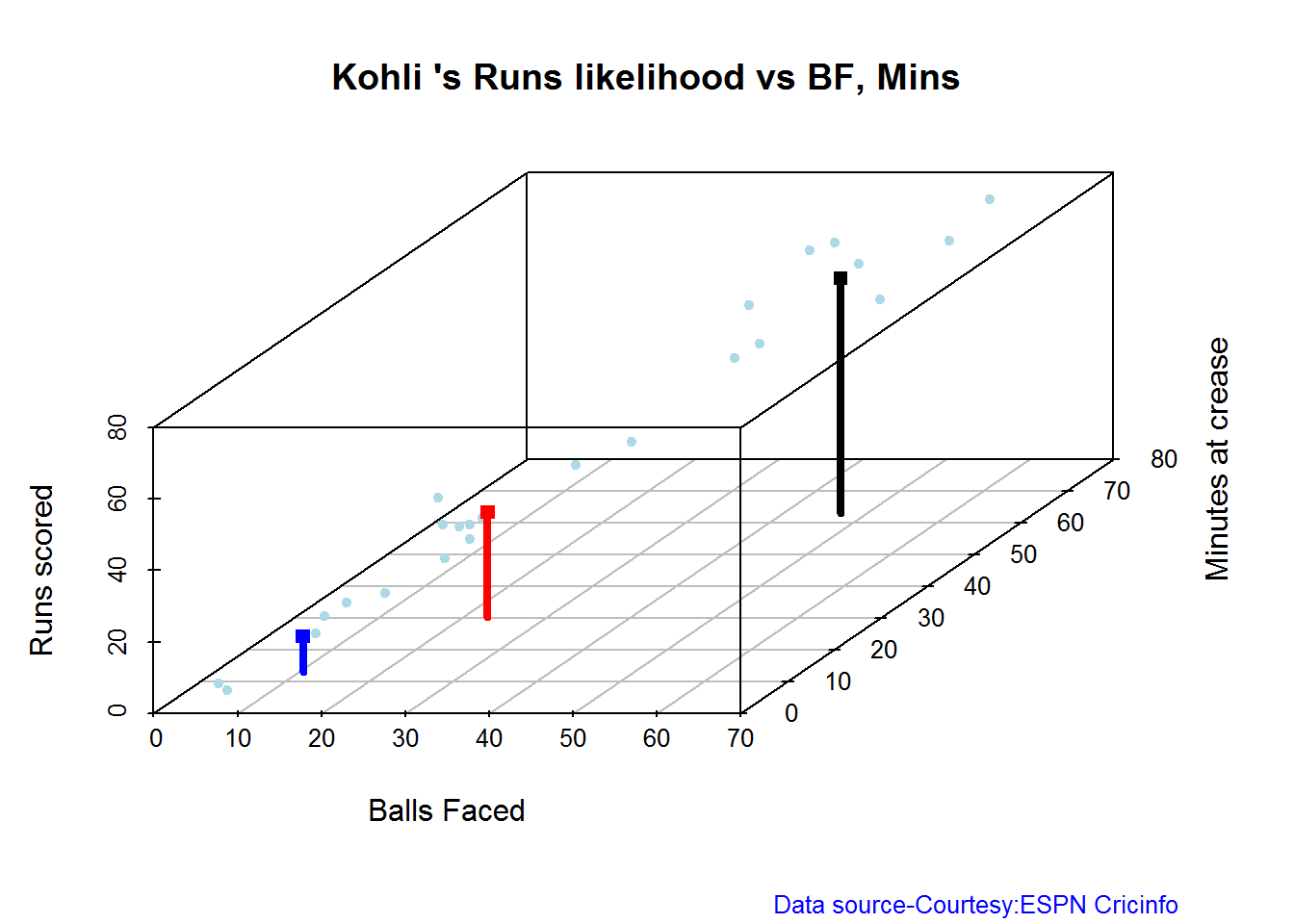
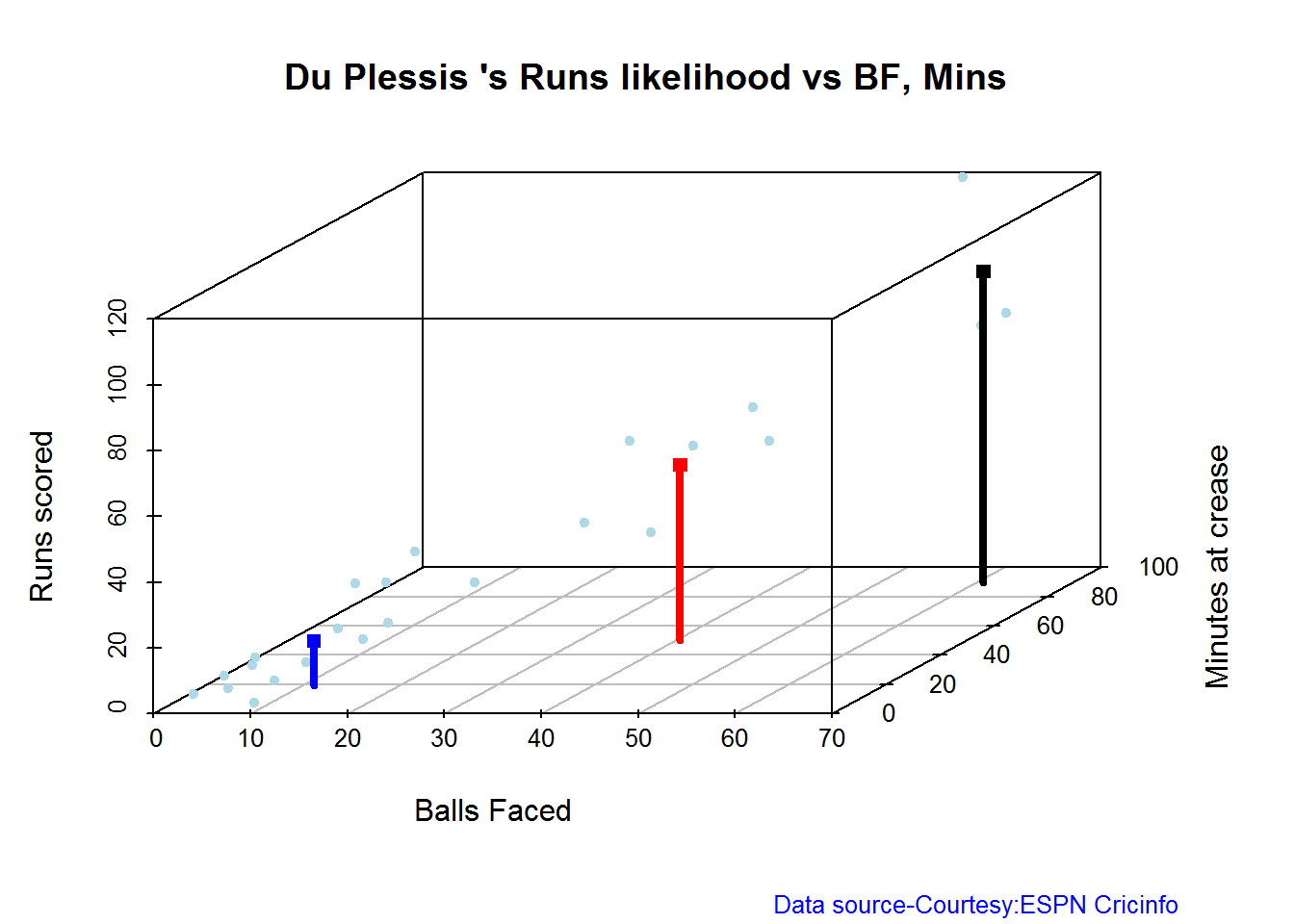
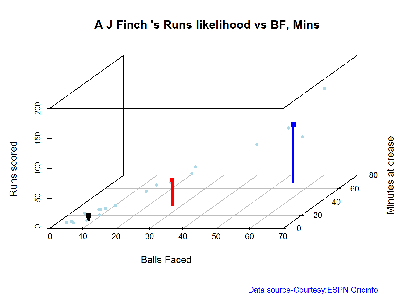
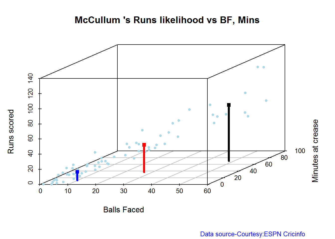
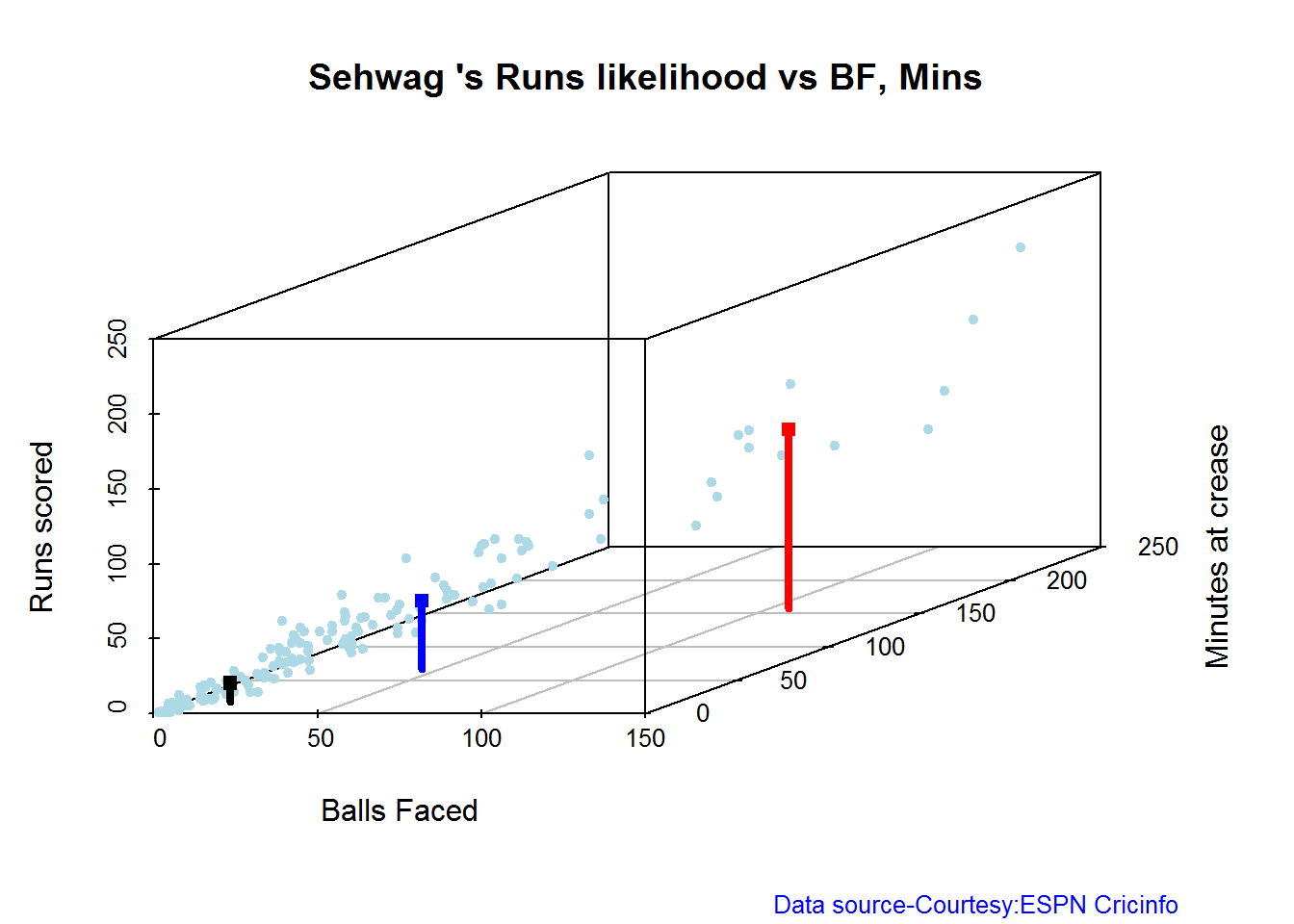
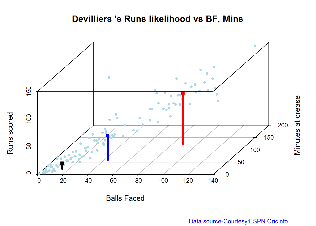
Highest runs likelihood
The plots below the runs likelihood of batsman. This uses K-Means It can be seen that Devilliers has almost 27.75% likelihood to make around 90+ runs. Gayle and Sehwag have 34% to make 40+ runs. A. Virender Sehwag
A. Virender Sehwag
batsmanRunsLikelihood("./sehwag.csv","Sehwag")

## Summary of Sehwag 's runs scoring likelihood
## **************************************************
##
## There is a 35.22 % likelihood that Sehwag will make 46 Runs in 44 balls over 67 Minutes
## There is a 9.43 % likelihood that Sehwag will make 119 Runs in 106 balls over 158 Minutes
## There is a 55.35 % likelihood that Sehwag will make 12 Runs in 13 balls over 18 Minutes
B. AB Devilliers
batsmanRunsLikelihood("./devilliers.csv","Devilliers")

## Summary of Devilliers 's runs scoring likelihood
## **************************************************
##
## There is a 30.65 % likelihood that Devilliers will make 44 Runs in 43 balls over 60 Minutes
## There is a 29.84 % likelihood that Devilliers will make 91 Runs in 88 balls over 124 Minutes
## There is a 39.52 % likelihood that Devilliers will make 11 Runs in 15 balls over 21 Minutes
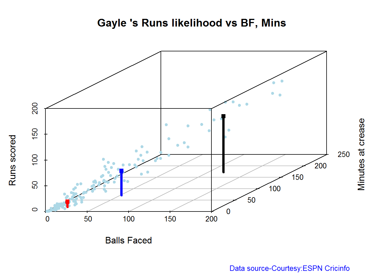
C. Chris Gayle
batsmanRunsLikelihood("./gayle.csv","Gayle")

## Summary of Gayle 's runs scoring likelihood
## **************************************************
##
## There is a 32.69 % likelihood that Gayle will make 47 Runs in 51 balls over 72 Minutes
## There is a 54.49 % likelihood that Gayle will make 10 Runs in 15 balls over 20 Minutes
## There is a 12.82 % likelihood that Gayle will make 109 Runs in 119 balls over 172 Minutes
D. Glenn Maxwell
batsmanRunsLikelihood("./maxwell.csv","Maxwell")

## Summary of Maxwell 's runs scoring likelihood
## **************************************************
##
## There is a 34.38 % likelihood that Maxwell will make 39 Runs in 29 balls over 35 Minutes
## There is a 15.62 % likelihood that Maxwell will make 89 Runs in 55 balls over 69 Minutes
## There is a 50 % likelihood that Maxwell will make 6 Runs in 7 balls over 9 Minutes
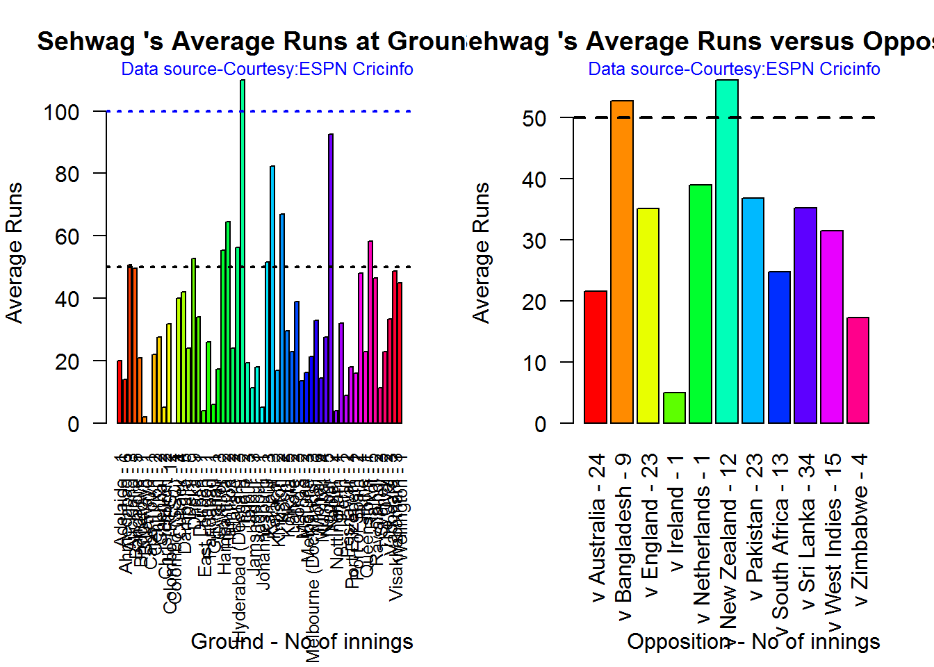
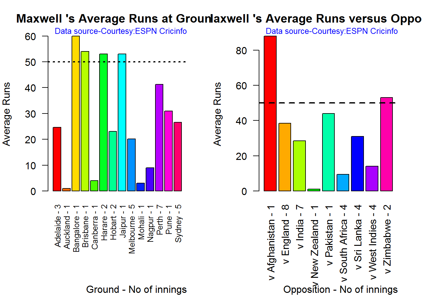
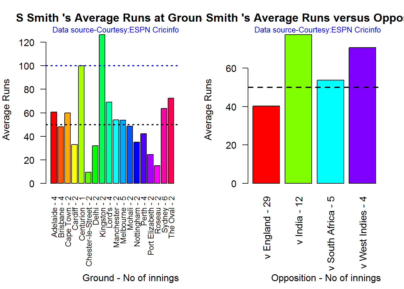
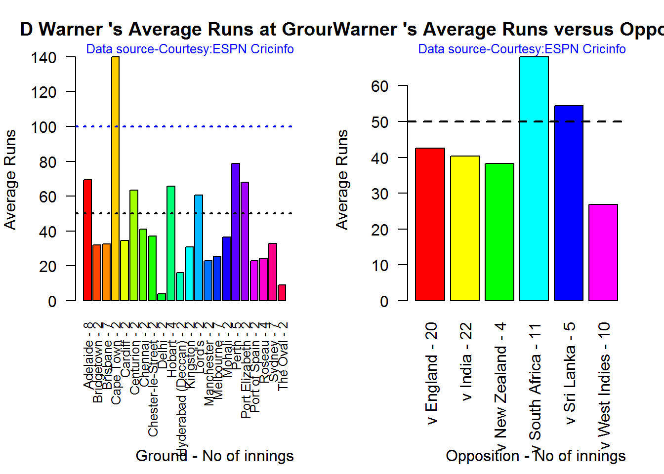
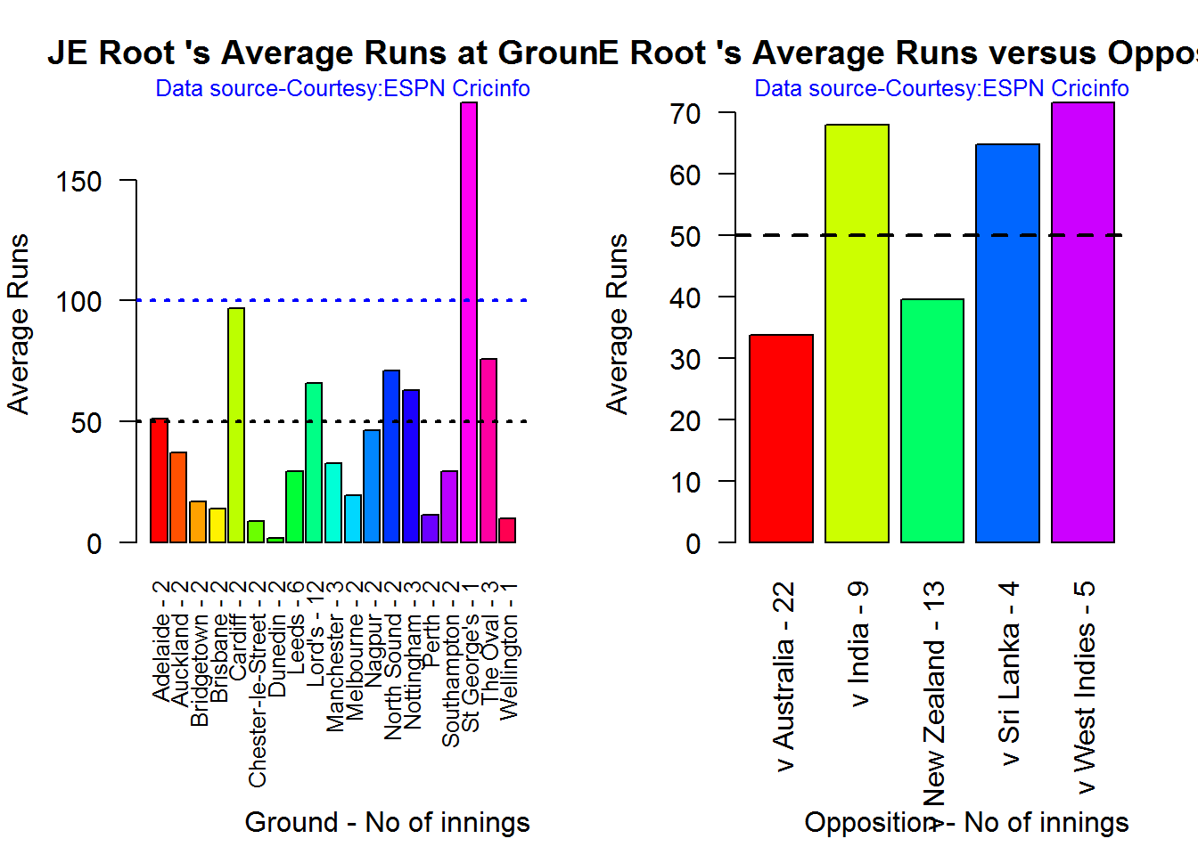
Average runs at ground and against opposition
A. Virender Sehwag
par(mfrow=c(1,2))
par(mar=c(4,4,2,2))
batsmanAvgRunsGround("./sehwag.csv","Sehwag")
batsmanAvgRunsOpposition("./sehwag.csv","Sehwag")

dev.off()
## null device
##           1
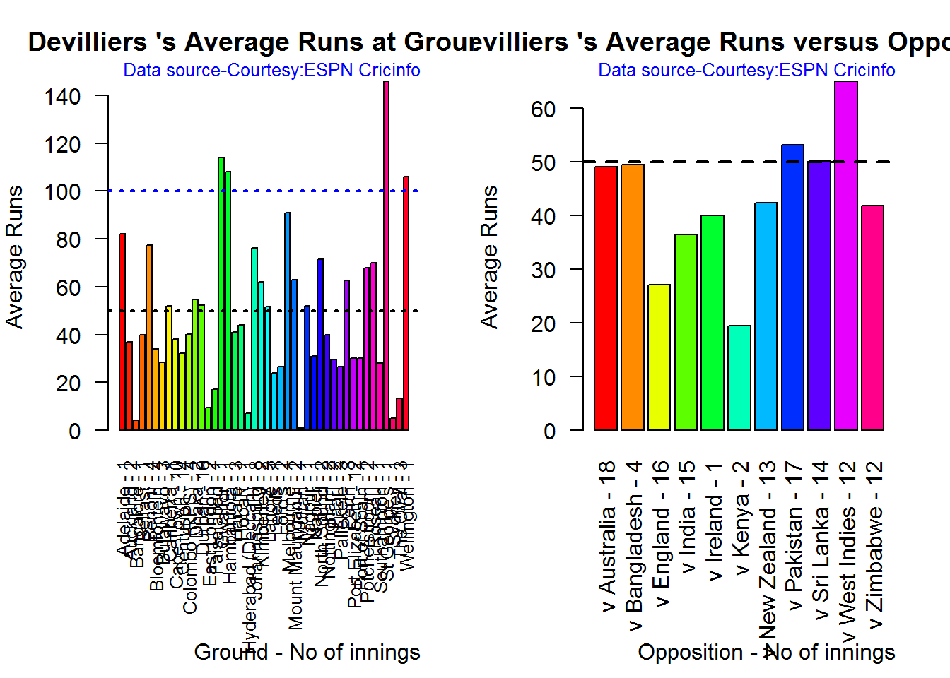
B. AB Devilliers
par(mfrow=c(1,2))
par(mar=c(4,4,2,2))
batsmanAvgRunsGround("./devilliers.csv","Devilliers")
batsmanAvgRunsOpposition("./devilliers.csv","Devilliers")

dev.off()
## null device
##           1
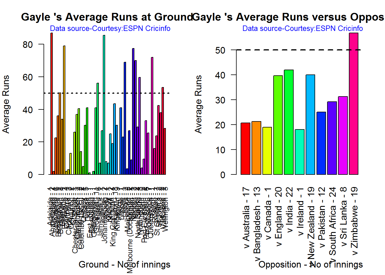
C. Chris Gayle
par(mfrow=c(1,2))
par(mar=c(4,4,2,2))
batsmanAvgRunsGround("./gayle.csv","Gayle")
batsmanAvgRunsOpposition("./gayle.csv","Gayle")

dev.off()
## null device
##           1
D. Glenn Maxwell
par(mfrow=c(1,2))
par(mar=c(4,4,2,2))
batsmanAvgRunsGround("./maxwell.csv","Maxwell")
batsmanAvgRunsOpposition("./maxwell.csv","Maxwell")

dev.off()
## null device
##           1
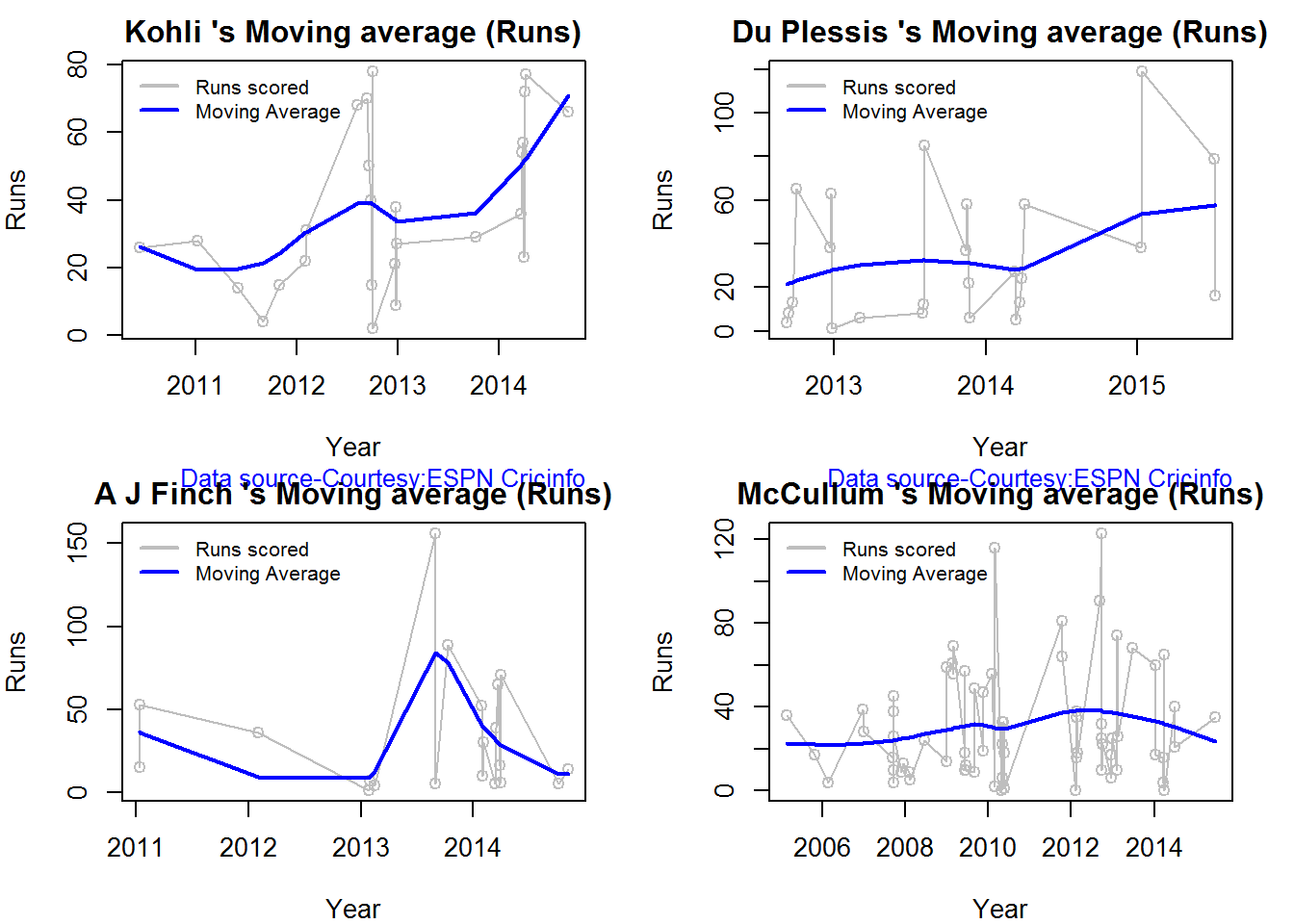
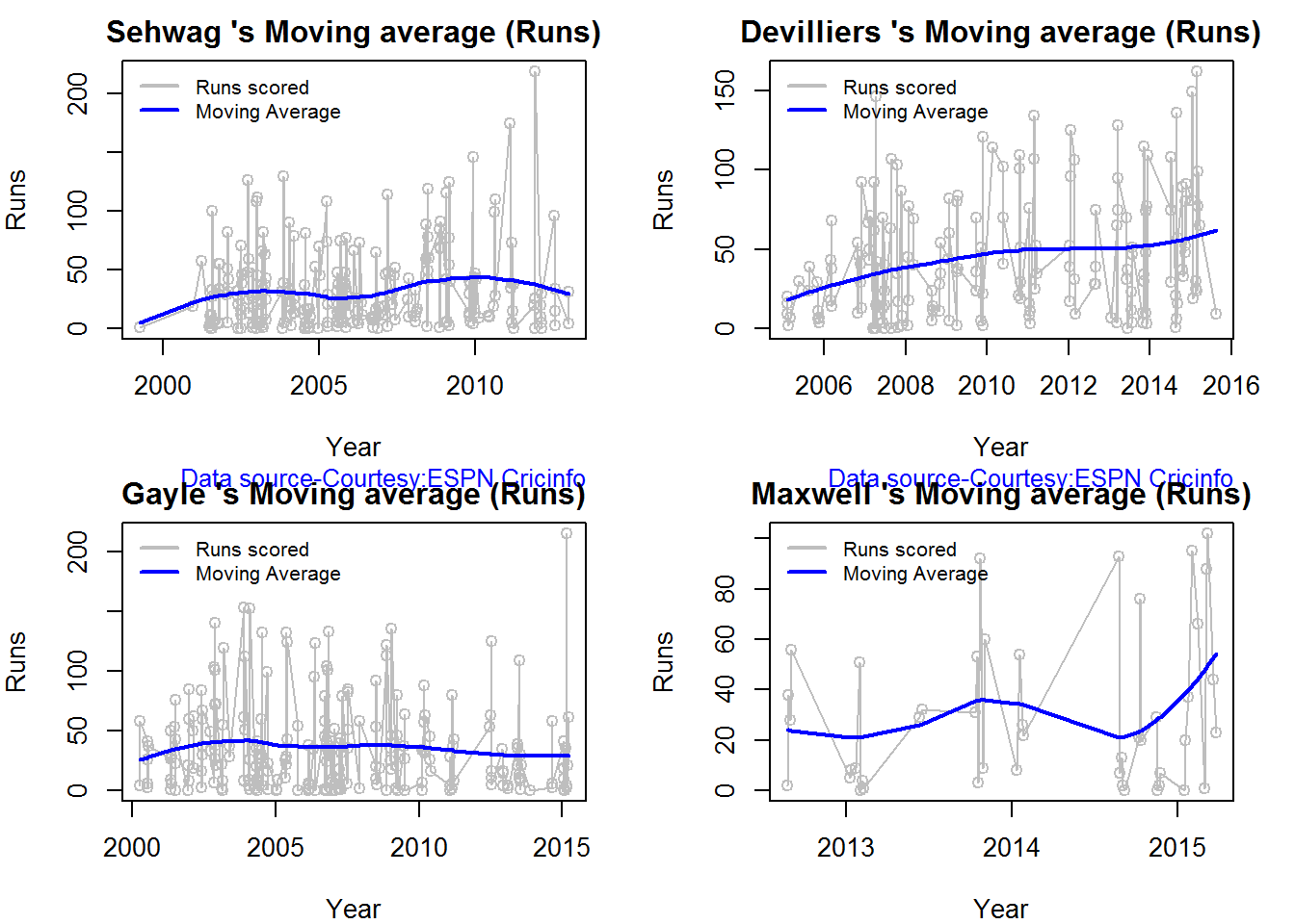
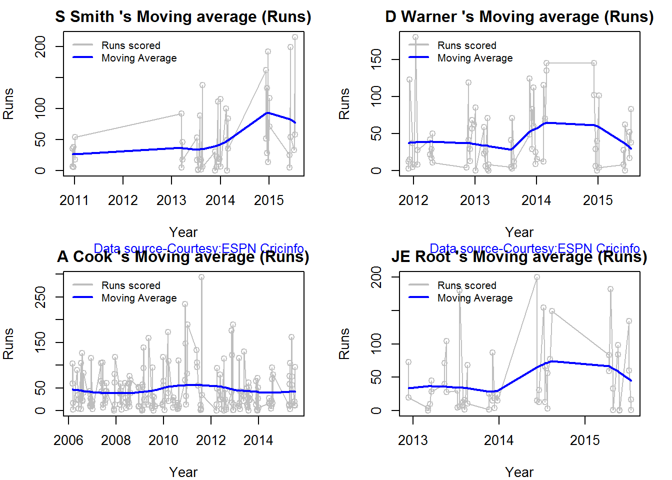
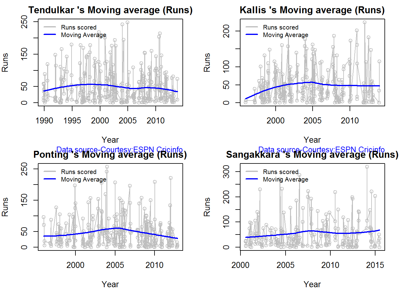
Moving Average of runs over career
The moving average for the 4 batsmen indicate the following
1. The moving average of Devilliers and Maxwell is on the way up.
2. Sehwag shows a slight downward trend from his 2nd peak in 2011
3. Gayle maintains a consistent 45 runs for the last few years
par(mfrow=c(2,2))
par(mar=c(4,4,2,2))
batsmanMovingAverage("./sehwag.csv","Sehwag")
batsmanMovingAverage("./devilliers.csv","Devilliers")
batsmanMovingAverage("./gayle.csv","Gayle")
batsmanMovingAverage("./maxwell.csv","Maxwell")

dev.off()
## null device
##           1
Analysis of bowlers
- Mitchell Johnson (Aus) – Innings-150, Wickets – 239, Econ Rate : 4.83
- Lasith Malinga (SL)- Innings-182, Wickets – 287, Econ Rate : 5.26
- Dale Steyn (SA)- Innings-103, Wickets – 162, Econ Rate : 4.81
- Tim Southee (NZ)- Innings-96, Wickets – 135, Econ Rate : 5.33
Malinga has the highest number of innings and wickets followed closely by Mitchell. Steyn and Southee have relatively fewer innings.
To get the bowler’s data use
malinga <- getPlayerDataOD(49758,dir=".",file="malinga.csv",type="bowling")
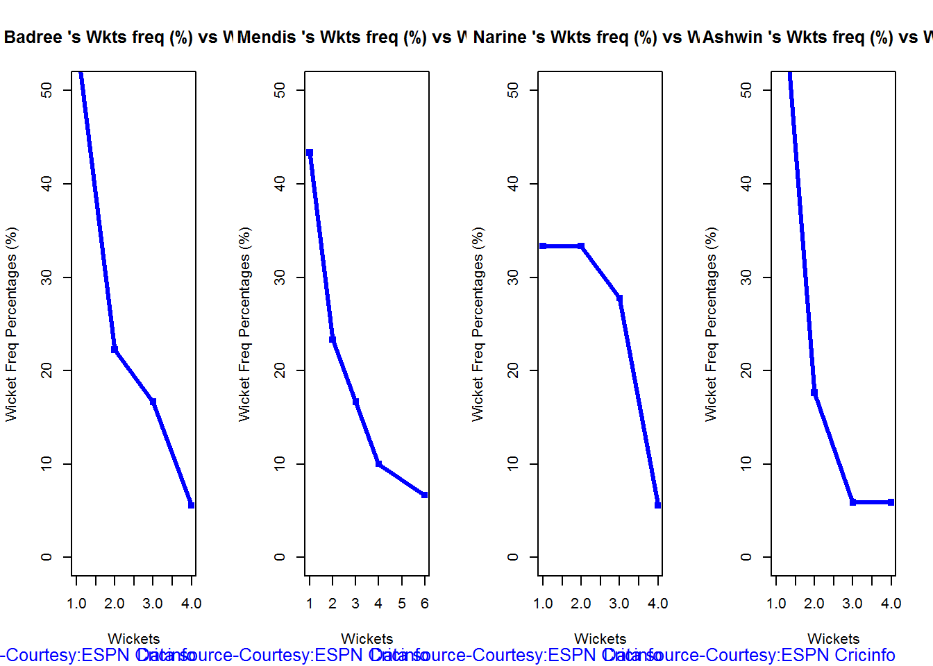
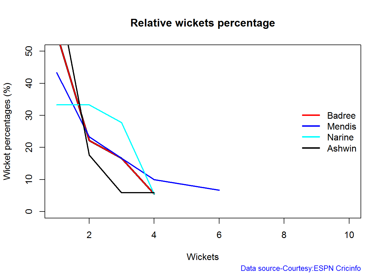
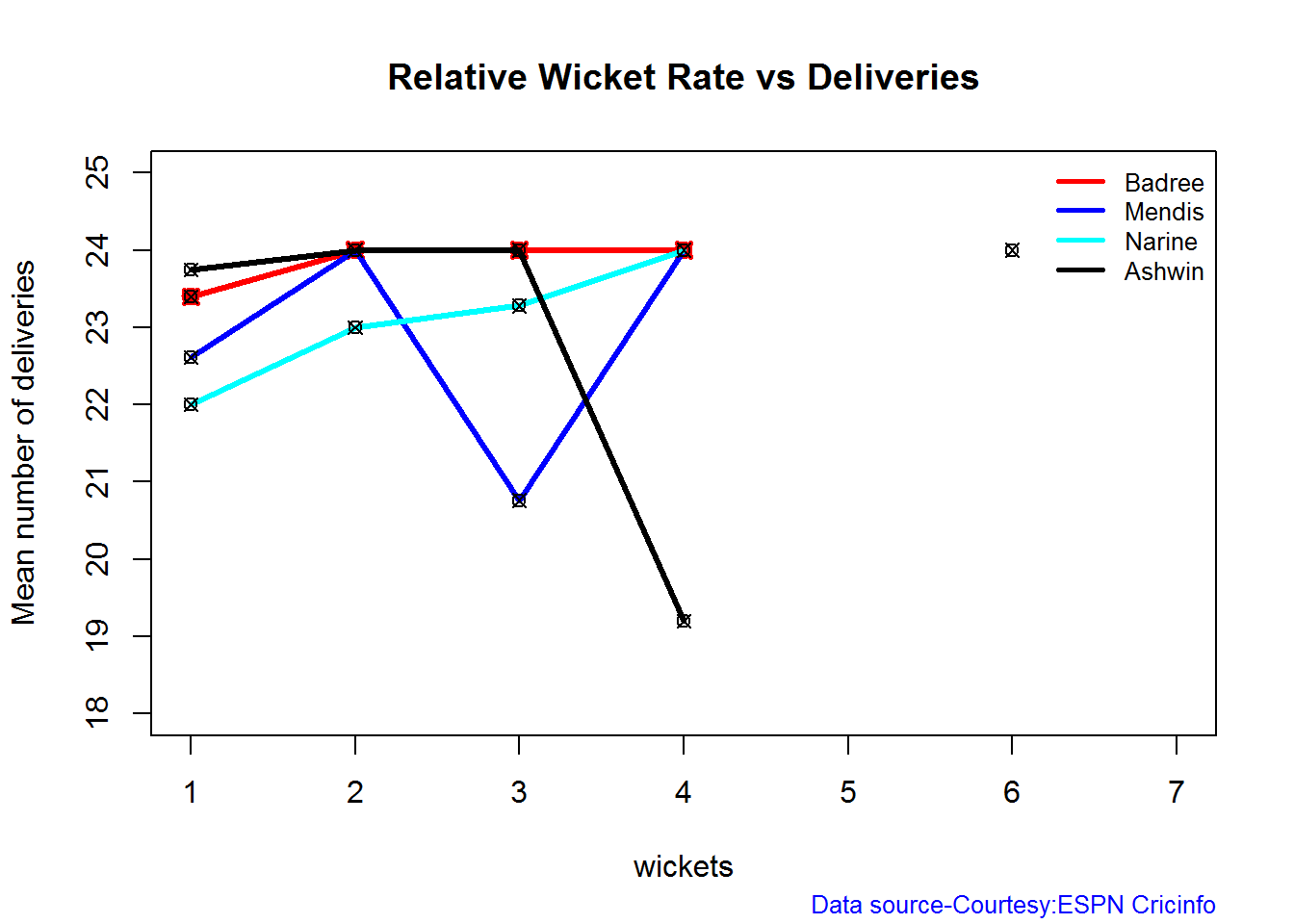
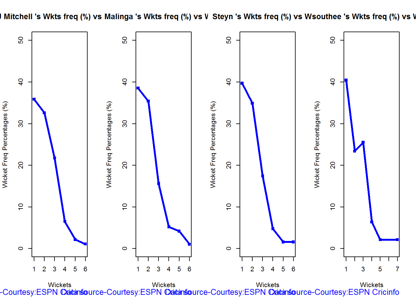
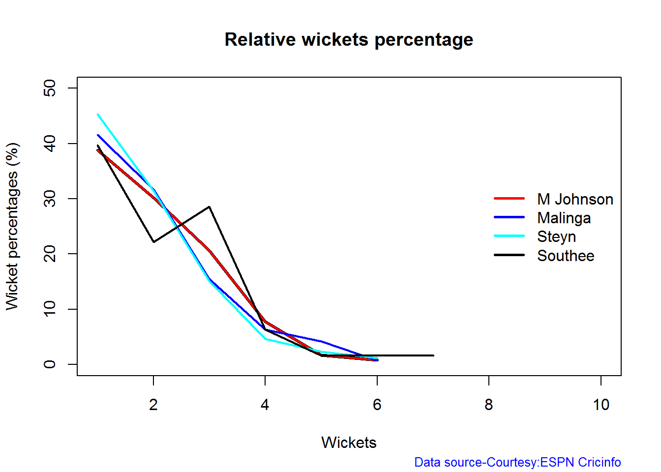
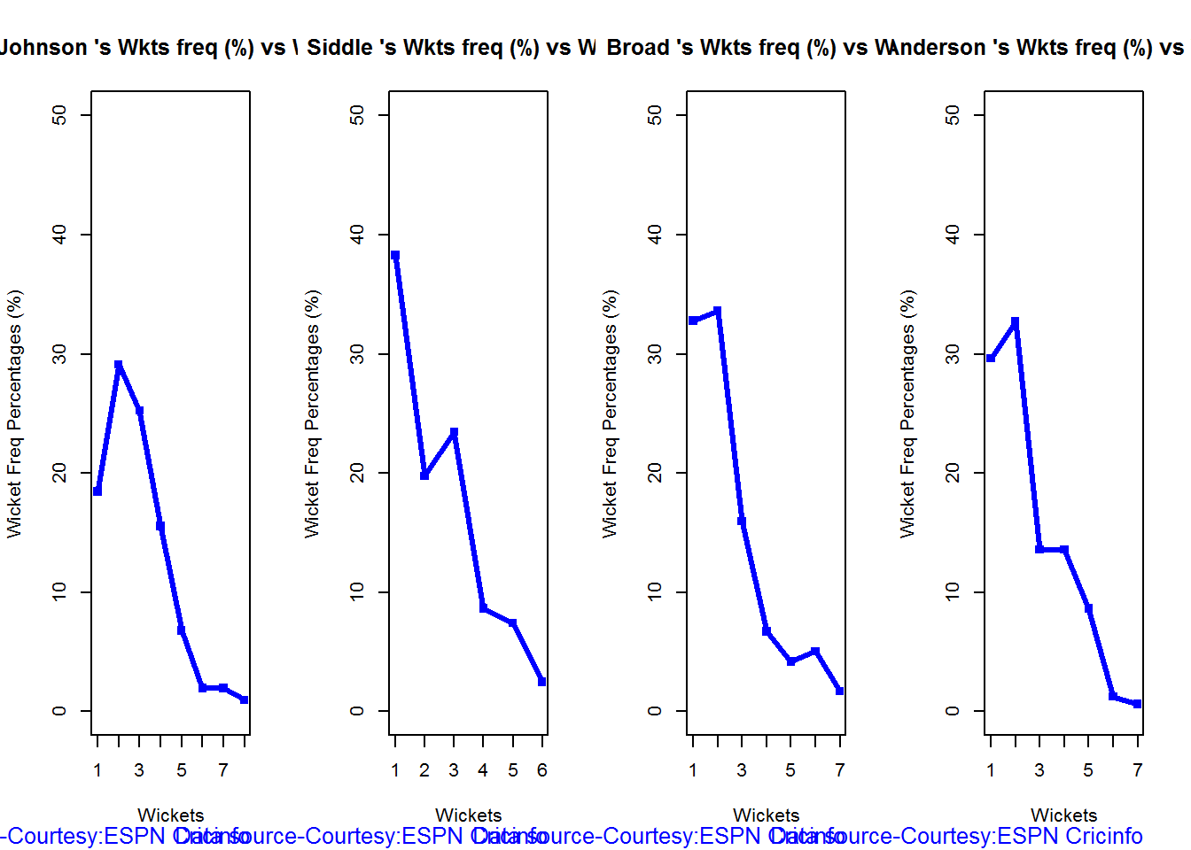
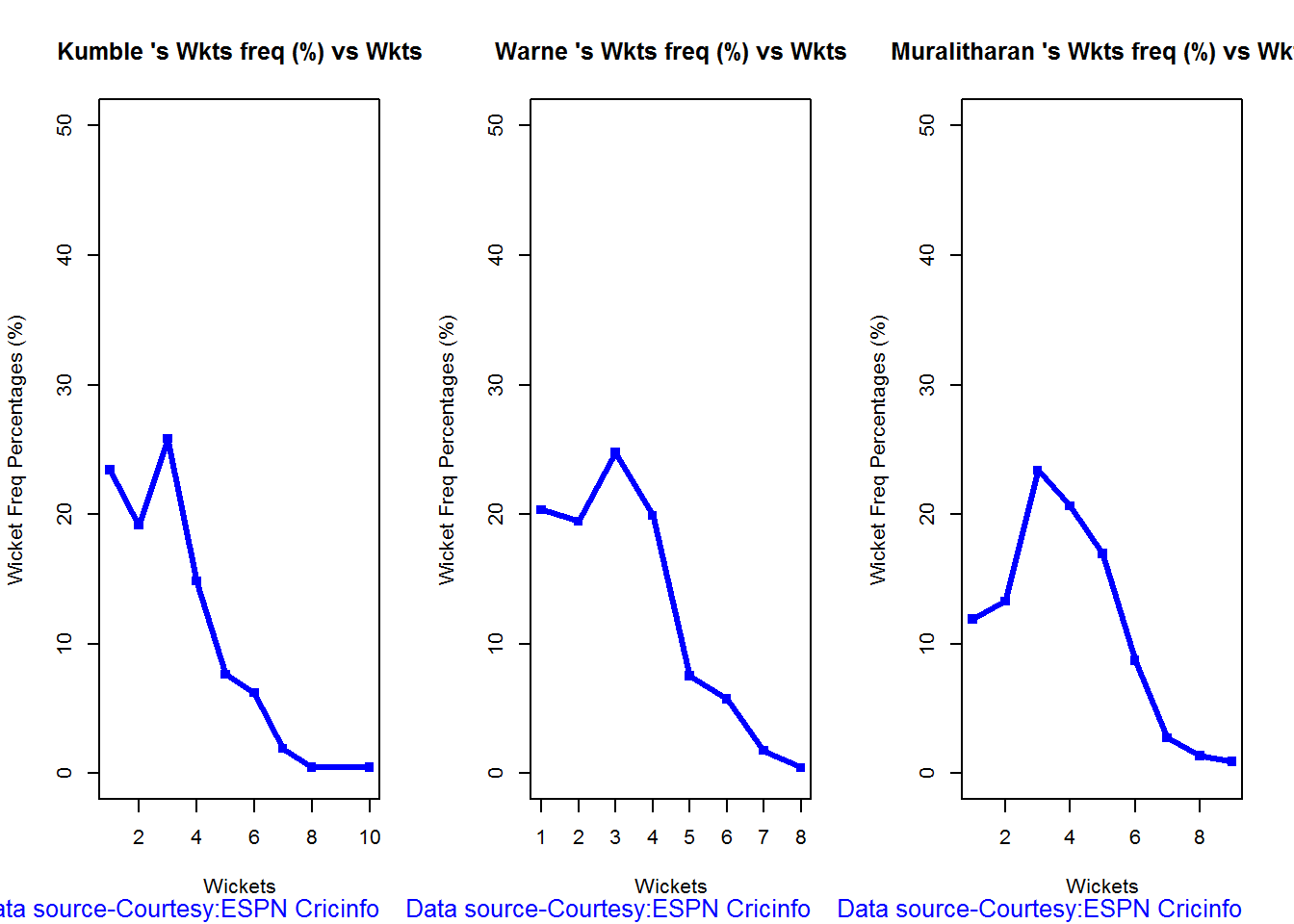
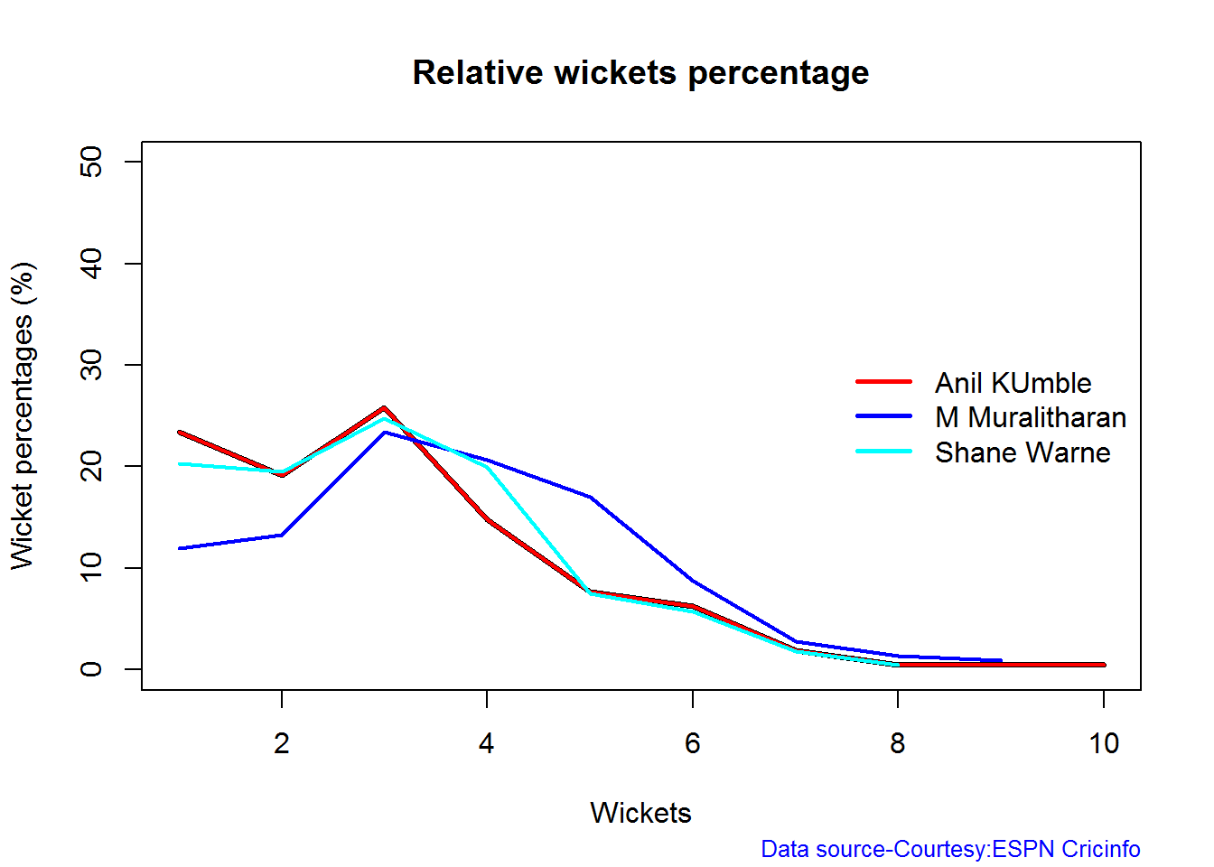
Wicket Frequency percentage
This plot gives the percentage of wickets for each wickets (1,2,3…etc)
par(mfrow=c(1,4))
par(mar=c(4,4,2,2))
bowlerWktsFreqPercent("./mitchell.csv","J Mitchell")
bowlerWktsFreqPercent("./malinga.csv","Malinga")
bowlerWktsFreqPercent("./steyn.csv","Steyn")
bowlerWktsFreqPercent("./southee.csv","southee")

dev.off()
## null device
##           1
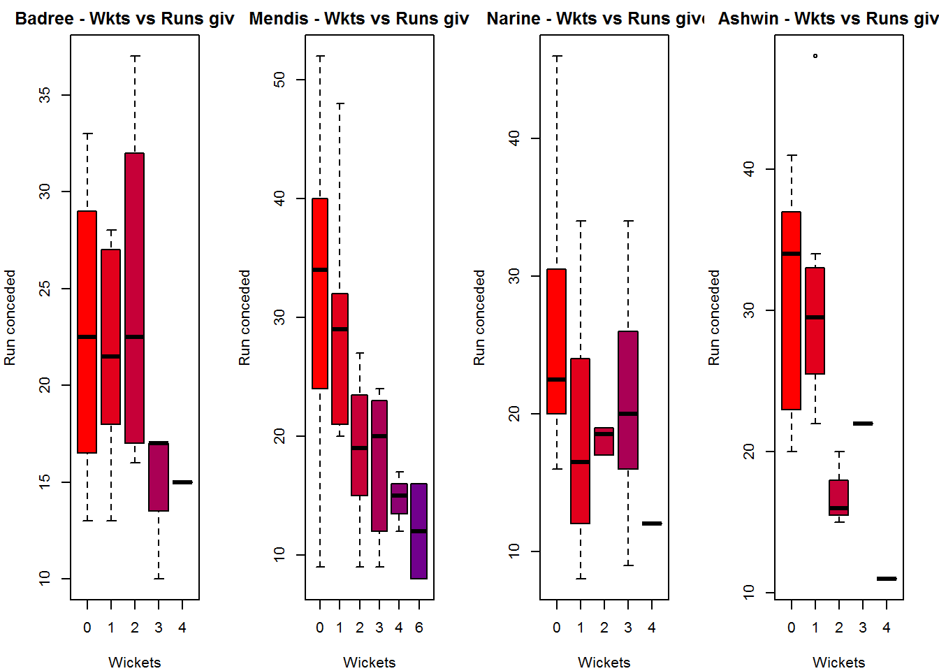
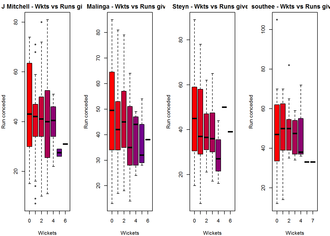
Wickets Runs plot
The plot below gives a boxplot of the runs ranges for each of the wickets taken by the bowlers. M Johnson and Steyn are more economical than Malinga and Southee corroborating the figures above
par(mfrow=c(1,4))
par(mar=c(4,4,2,2))
bowlerWktsRunsPlot("./mitchell.csv","J Mitchell")
bowlerWktsRunsPlot("./malinga.csv","Malinga")
bowlerWktsRunsPlot("./steyn.csv","Steyn")
bowlerWktsRunsPlot("./southee.csv","southee")

dev.off()
## null device
##           1
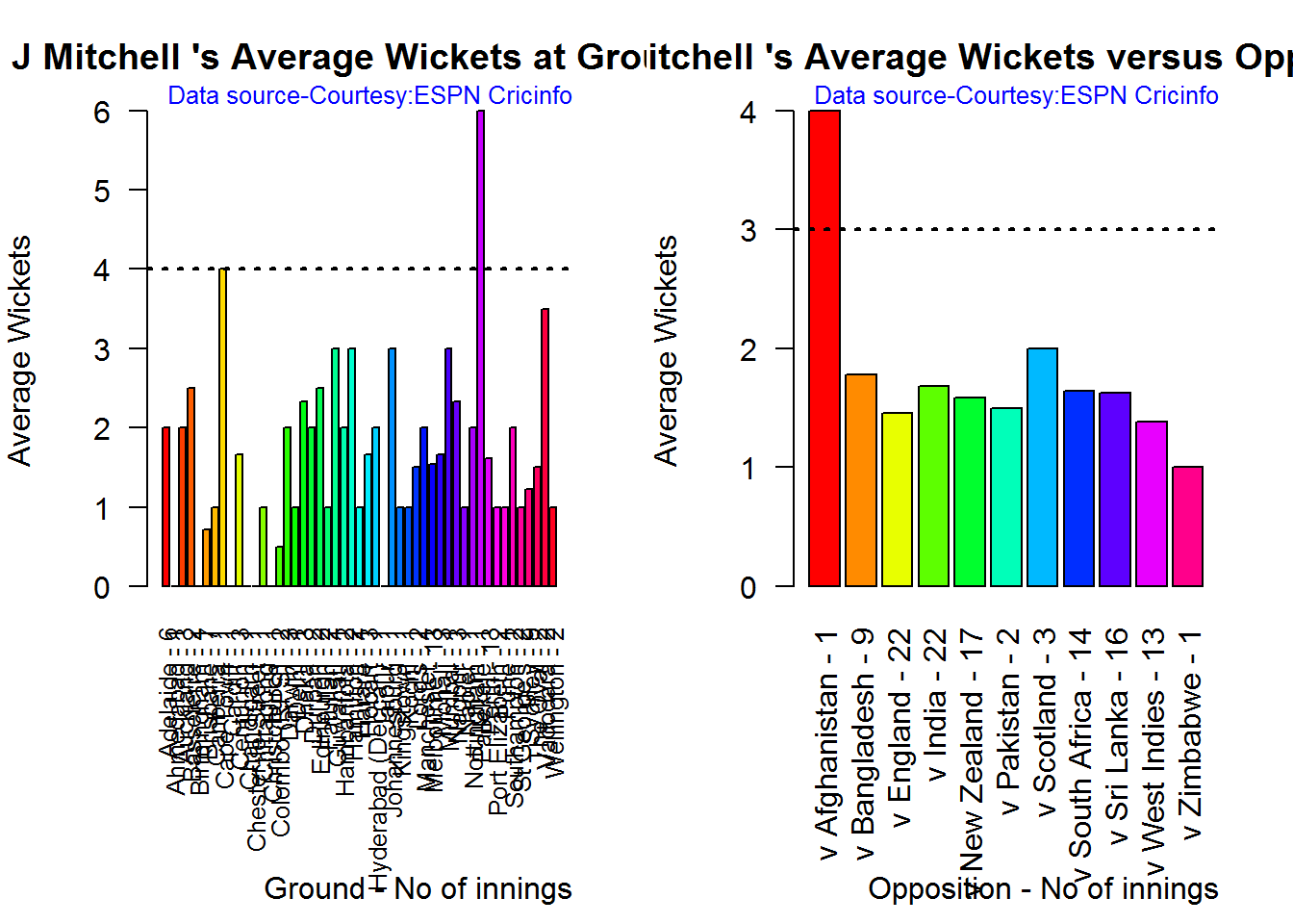
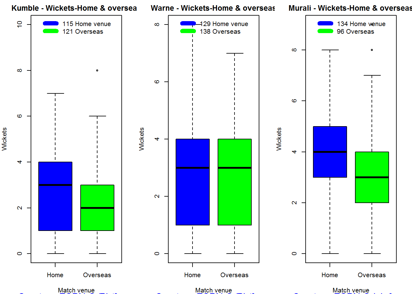
Average wickets in different grounds and opposition
A. Mitchell Johnson
par(mfrow=c(1,2))
par(mar=c(4,4,2,2))
bowlerAvgWktsGround("./mitchell.csv","J Mitchell")
bowlerAvgWktsOpposition("./mitchell.csv","J Mitchell")

dev.off()
## null device
##           1
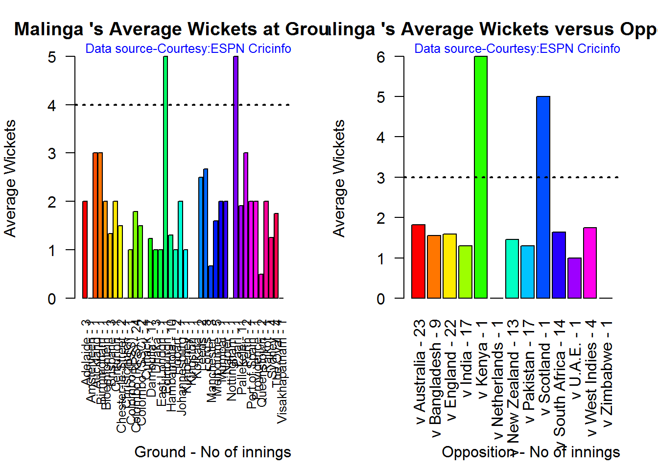
B. Lasith Malinga
par(mfrow=c(1,2))
par(mar=c(4,4,2,2))
bowlerAvgWktsGround("./malinga.csv","Malinga")
bowlerAvgWktsOpposition("./malinga.csv","Malinga")

dev.off()
## null device
##           1
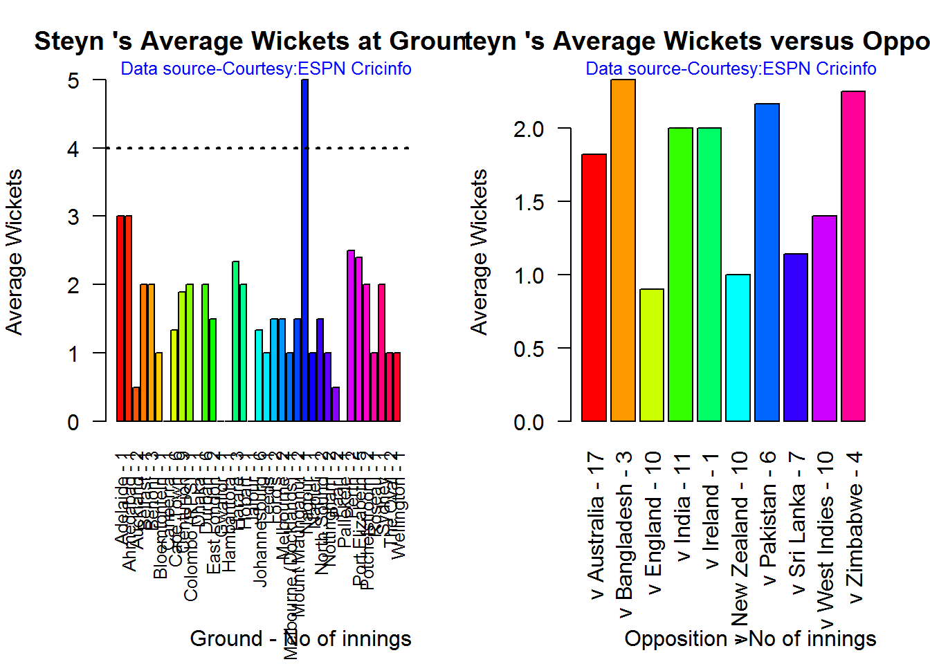
C. Dale Steyn
par(mfrow=c(1,2))
par(mar=c(4,4,2,2))
bowlerAvgWktsGround("./steyn.csv","Steyn")
bowlerAvgWktsOpposition("./steyn.csv","Steyn")

dev.off()
## null device
##           1
D. Tim Southee
par(mfrow=c(1,2))
par(mar=c(4,4,2,2))
bowlerAvgWktsGround("./southee.csv","southee")
bowlerAvgWktsOpposition("./southee.csv","southee")

dev.off()
## null device
##           1
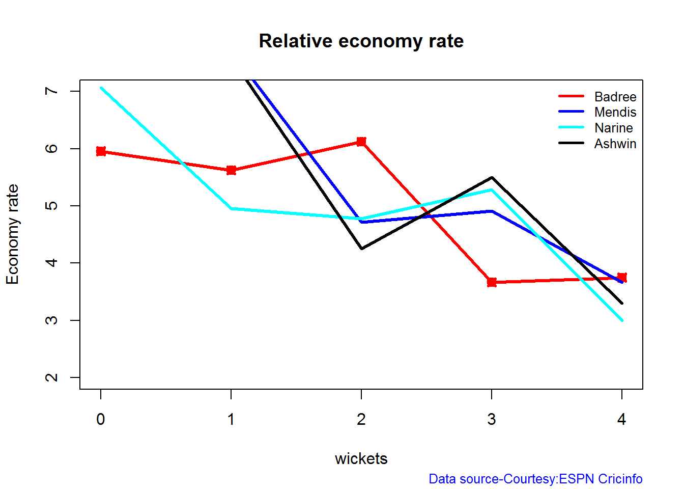
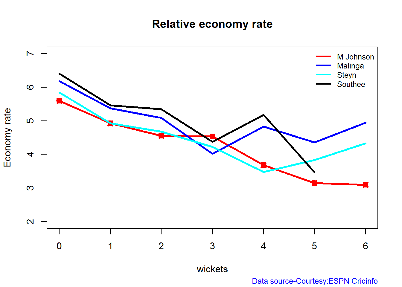
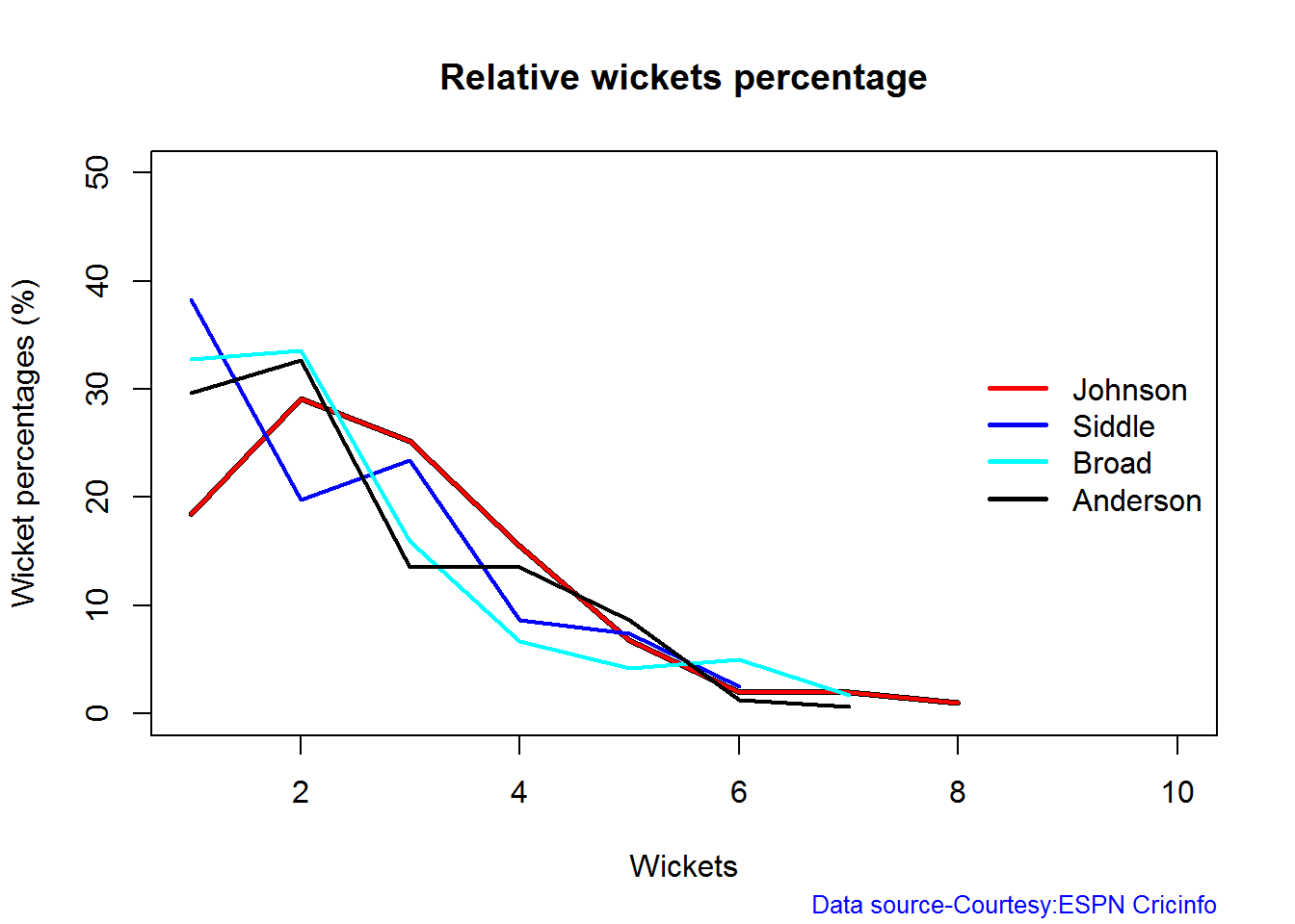
Relative Economy Rate against wickets taken
Steyn had the best economy rate followed by M Johnson. Malinga and Southee have a poorer economy rate
frames <- list("./mitchell.csv","./malinga.csv","steyn.csv","southee.csv")
names <- list("M Johnson","Malinga","Steyn","Southee")
relativeBowlingERODTT(frames,names)

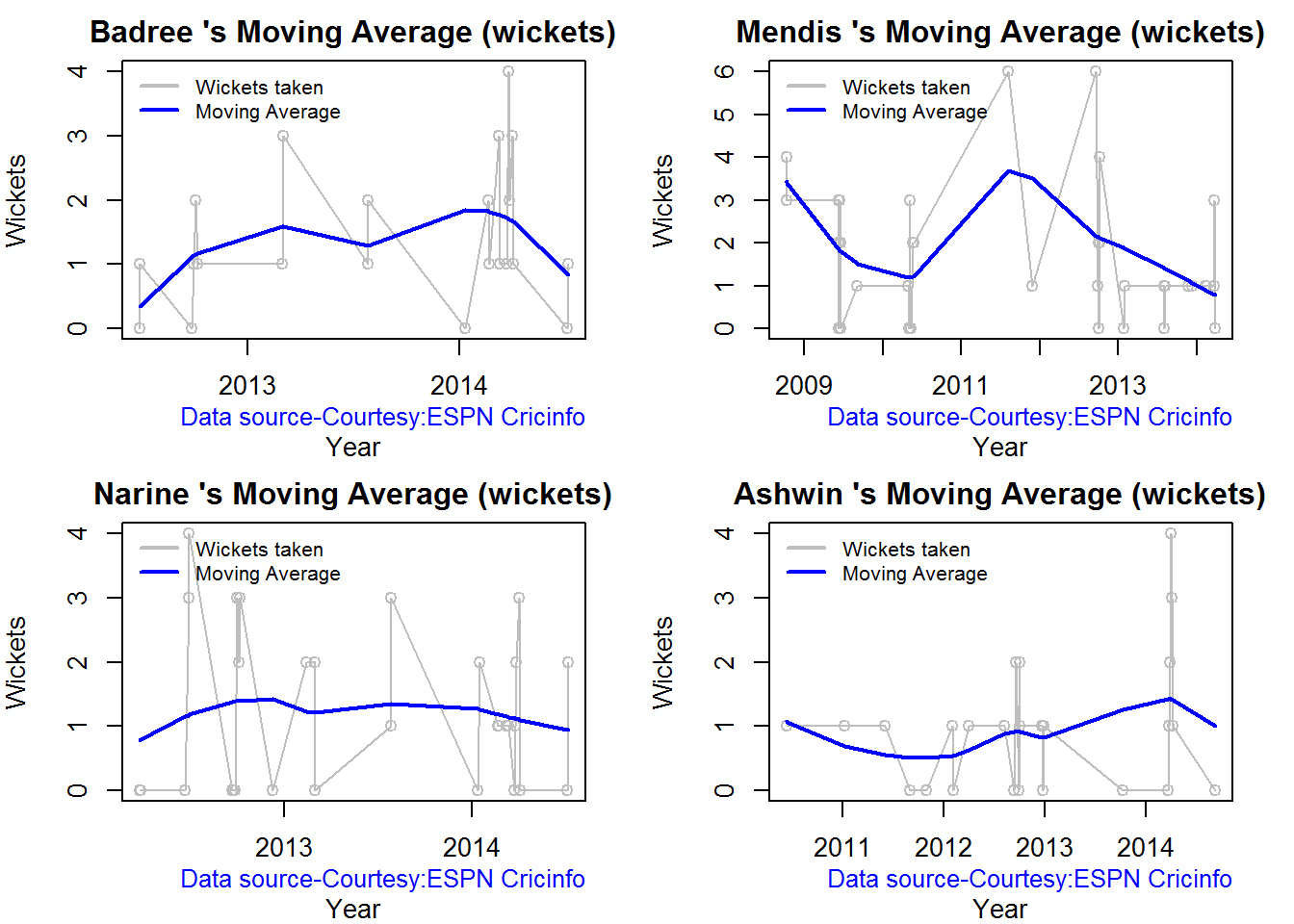
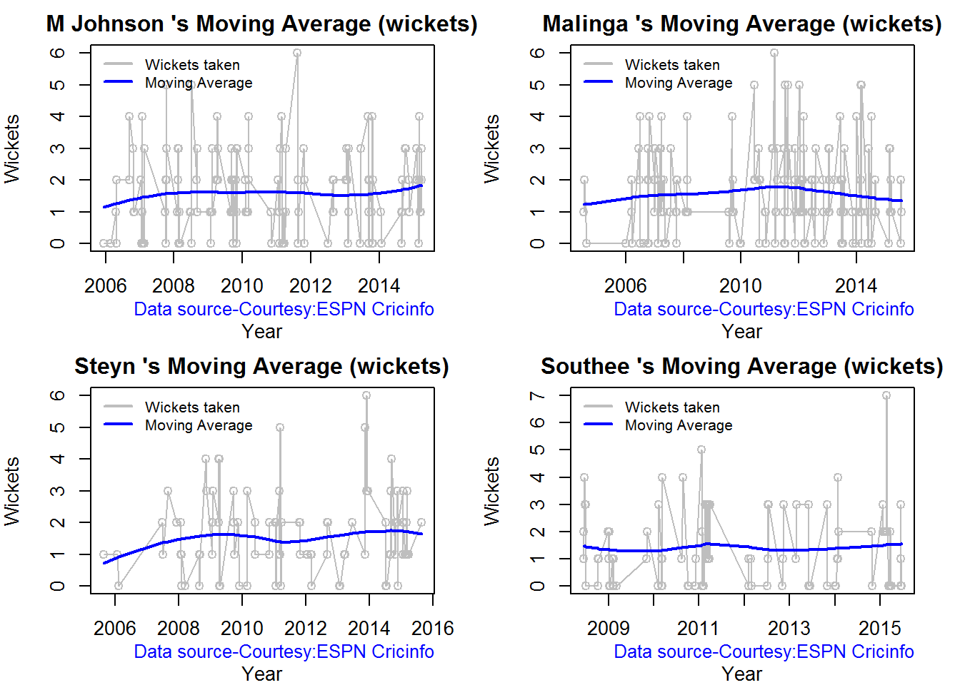
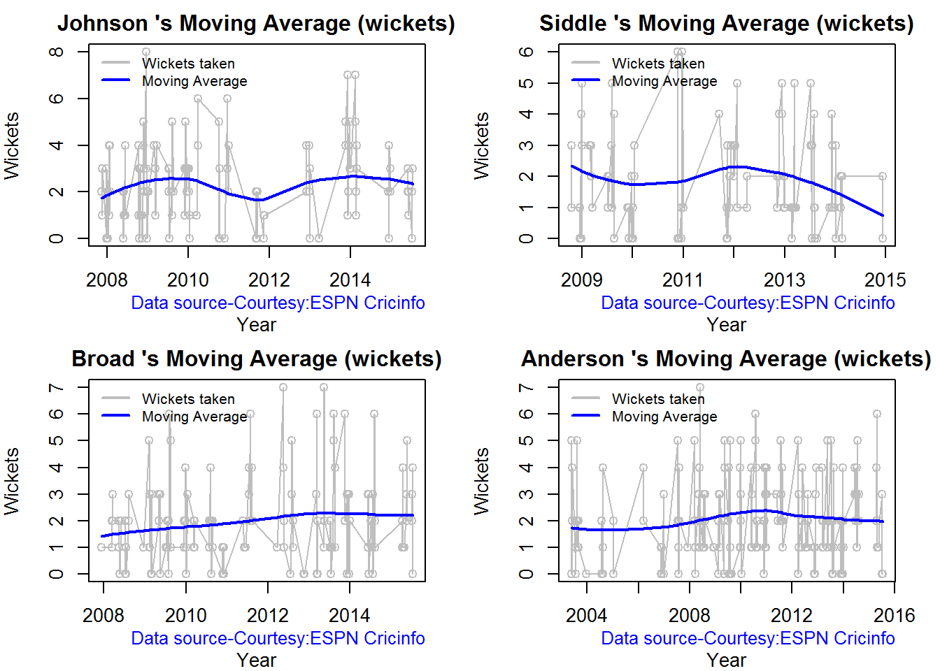
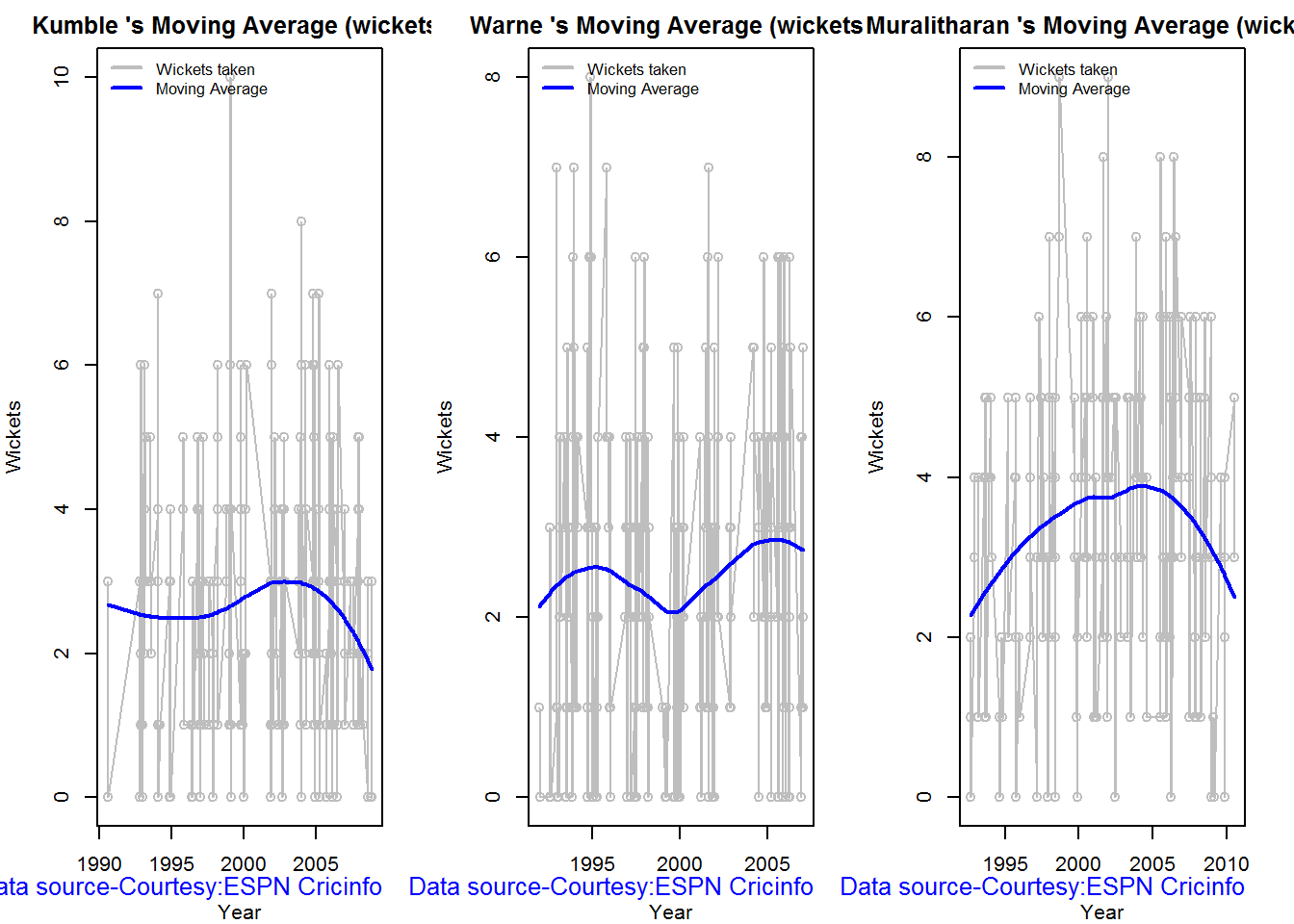
Moving average of wickets over career
Johnson and Steyn career vs wicket graph is on the up-swing. Southee is maintaining a reasonable record while Malinga shows a decline in ODI performance
par(mfrow=c(2,2))
par(mar=c(4,4,2,2))
bowlerMovingAverage("./mitchell.csv","M Johnson")
bowlerMovingAverage("./malinga.csv","Malinga")
bowlerMovingAverage("./steyn.csv","Steyn")
bowlerMovingAverage("./southee.csv","Southee")

dev.off()
## null device
##           1
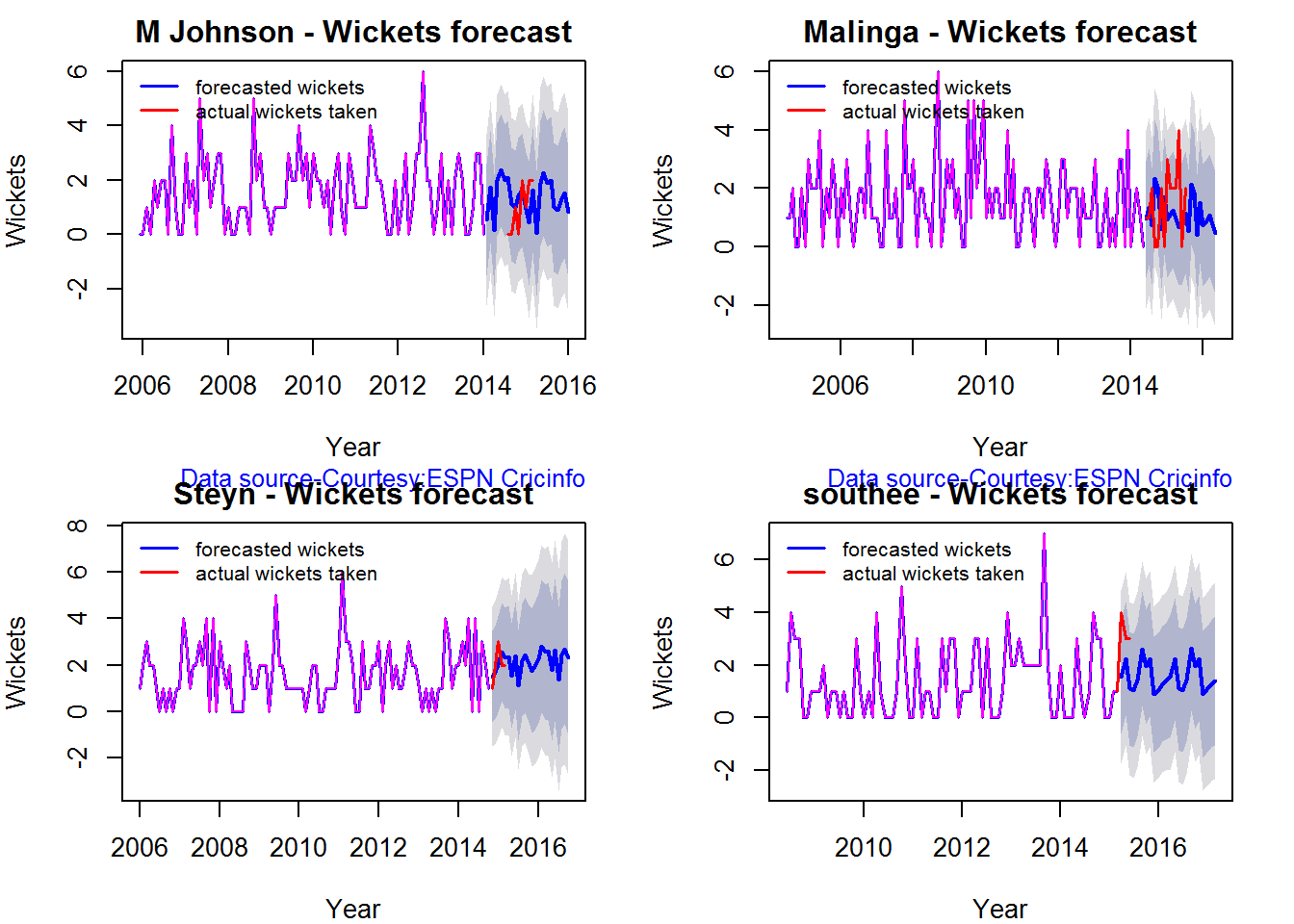
Wickets forecast
par(mfrow=c(2,2))
par(mar=c(4,4,2,2))
bowlerPerfForecast("./mitchell.csv","M Johnson")
bowlerPerfForecast("./malinga.csv","Malinga")
bowlerPerfForecast("./steyn.csv","Steyn")
bowlerPerfForecast("./southee.csv","southee")

dev.off()
## null device
##           1


 Checkout my book ‘Deep Learning from first principles- In vectorized Python, R and Octave’. My book is available on Amazon as