Introduction
In this post (The making of cricket package yorkr-Part 2), I continue to add new functionality to my package cricket package yorkr in R. In my earlier post The making of cricket package yorkr-Part 1 I had included functionality that will plot batsman partnerships, bowlers performances with wicket-kind, wicket-runs in specified ODI match. The earlier post also included functions that were based on confrontations between any 2 teams ( I had chosen the ODI matches between India and Australia).
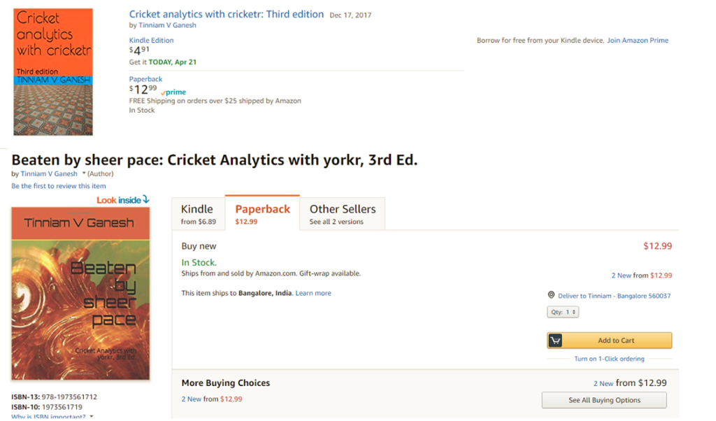
If you are passionate about cricket, and love analyzing cricket performances, then check out my 2 racy books on cricket! In my books, I perform detailed yet compact analysis of performances of both batsmen, bowlers besides evaluating team & match performances in Tests , ODIs, T20s & IPL. You can buy my books on cricket from Amazon at $12.99 for the paperback and $4.99/$6.99 respectively for the kindle versions. The books can be accessed at Cricket analytics with cricketr and Beaten by sheer pace-Cricket analytics with yorkr A must read for any cricket lover! Check it out!!
320 and $6.99/Rs448 respectively
Checkout my interactive Shiny apps GooglyPlus (plots & tables) and Googly (only plots) which can be used to analyze IPL players, teams and matches.
Important note: Do check out all the posts on the python avatar of yorkr, namely ‘yorkpy’ in my post ‘Pitching yorkpy … short of good length to IPL – Part 1”
This post includes all ODI matches between a country and others. For obvious reasons I have chosen India and selected all ODI matches played by India with other countries. As mentioned in my earlier post the data is taken from Cricsheet. There are a total of 262 ODI matches that India has played. These 262 ODI matches played by India are then combined into one large dataframe that is 140,655 rows x 22 columns.
The analysis is then done on India’s batting and bowling performances on this huge dataframe for e.g. who has the most scores and highest batting partnerships, which bowlers are most effective against a country. Also the functions give details like which Indian bowlers have the worst performance or which bowlers have taken the most wicket against India. The functions also provide information on batsmen and bowlers of the opposing countries who have performed welll against India. Since the dataset is large and rich, the possible insights are infinite.I am including some functions that I have created on this dataset below.
Also note that it is possible to choose all ODI matches played by Australia, Pakistan, South Africa etc with the rest of the world. Similar analysis can be done for these countries also by using the functions below
As before the package ‘yorkr’ is still under development. I will be releasing the package and code in about 6-10 weeks time. Please be patient.
This post is also available at RPubs at yorkr-2. You can download this post as a PDF document at yorkr-2.pdf
My earlier package ‘cricketr’ (see Introducing cricketr: An R package for analyzing performances of cricketers) was based on data from ESPN Cricinfo Statsguru. Take a look at my book with all my articles based on my package cricketr at – Cricket analytics with cricketr!!!. The book is also available in paperback and kindle versions at Amazon which has, by the way, better formatting!
library(dplyr)
library(ggplot2)
library(yorkr)
matches <- getAllMatches("India",save=FALSE)
dim(matches)
## [1] 140655 22
1. Team Batting details – India
The following function provides the overall batting performance of India against all opposition
Virat Kohli has the best performance with a total of 7023 runs in ODIs followed closely by Mahendra Dhoni with 6885 runs and then Suresh Raina with 4964 runs While Kohli leads in the numnber of 4s (662), Dhoni and Raina has twice the number of 6s as compared to Kohli. However Kohli has a better strike rate (7023/774100) = 90.33% while Dhoni has an overall strike rate of (6885/7878100) = 87.39%
df <-teamBattingDetailsAllOppn(matches,theTeam="India")
## Total= 58033
df
## Source: local data frame [71 x 5]
##
## batsman ballsPlayed fours sixes runs
## (fctr) (int) (int) (int) (dbl)
## 1 V Kohli 7774 662 65 7023
## 2 MS Dhoni 7878 515 129 6885
## 3 SK Raina 5076 429 114 4964
## 4 G Gambhir 5138 470 15 4495
## 5 RG Sharma 5245 370 89 4377
## 6 SR Tendulkar 4708 504 43 4196
## 7 Yuvraj Singh 4472 403 96 3976
## 8 V Sehwag 3102 494 74 3679
## 9 S Dhawan 2956 314 37 2694
## 10 AM Rahane 2490 194 24 2005
## .. ... ... ... ... ...
2. Team batting details – Other countries against India
When we use other countries in theTeam then we get the performance of batsman of these countries against India in ODIs. This is because matches is a selection of all matches played by India against other countries. The following there calls show the performances of the batsman of England, South Africa, Pakistan & Ireland against India.
df <-teamBattingDetailsAllOppn(matches,theTeam="England")
## Total= 7602
df
## Source: local data frame [43 x 5]
##
## batsman ballsPlayed fours sixes runs
## (fctr) (int) (int) (int) (dbl)
## 1 IR Bell 1238 110 9 1085
## 2 KP Pietersen 990 89 10 847
## 3 AN Cook 1049 103 2 822
## 4 RS Bopara 632 42 8 534
## 5 PD Collingwood 450 38 6 393
## 6 OA Shah 394 40 7 385
## 7 IJL Trott 410 33 2 349
## 8 JE Root 408 32 4 336
## 9 SR Patel 336 25 10 329
## 10 C Kieswetter 309 34 13 313
## .. ... ... ... ... ...
df <-teamBattingDetailsAllOppn(matches,theTeam="South Africa")
## Total= 6172
df
## Source: local data frame [36 x 5]
##
## batsman ballsPlayed fours sixes runs
## (fctr) (int) (int) (int) (dbl)
## 1 AB de Villiers 1026 102 38 1179
## 2 HM Amla 796 74 1 704
## 3 Q de Kock 637 76 8 633
## 4 JH Kallis 666 50 4 554
## 5 JP Duminy 477 19 9 438
## 6 F du Plessis 470 30 8 421
## 7 GC Smith 355 25 3 252
## 8 HH Gibbs 318 26 3 242
## 9 MN van Wyk 270 23 1 202
## 10 DA Miller 188 19 4 193
## .. ... ... ... ... ...
df <-teamBattingDetailsAllOppn(matches,theTeam="Pakistan")
## Total= 4660
df
## Source: local data frame [37 x 5]
##
## batsman ballsPlayed fours sixes runs
## (fctr) (int) (int) (int) (dbl)
## 1 Younis Khan 752 56 8 686
## 2 Shoaib Malik 669 61 4 595
## 3 Misbah-ul-Haq 619 49 6 550
## 4 Salman Butt 617 69 4 535
## 5 Mohammad Yousuf 458 37 2 432
## 6 Nasir Jamshed 473 41 4 408
## 7 Mohammad Hafeez 423 36 3 347
## 8 Shahid Afridi 187 16 7 235
## 9 Kamran Akmal 235 20 5 192
## 10 Umar Akmal 146 7 2 103
## .. ... ... ... ... ...
df <-teamBattingDetailsAllOppn(matches,theTeam="Bangladesh")
## Total= 3761
df
## Source: local data frame [39 x 5]
##
## batsman ballsPlayed fours sixes runs
## (fctr) (int) (int) (int) (dbl)
## 1 Mushfiqur Rahim 658 34 13 517
## 2 Tamim Iqbal 573 61 6 504
## 3 Shakib Al Hasan 591 42 5 493
## 4 Mahmudullah 310 27 1 269
## 5 Raqibul Hasan 262 11 3 202
## 6 Nasir Hossain 187 21 1 183
## 7 Mohammad Ashraful 235 17 NA 158
## 8 Soumya Sarkar 164 18 5 157
## 9 Imrul Kayes 183 21 1 155
## 10 Sabbir Rahman 142 16 1 136
## .. ... ... ... ... ...
3. Top batting partnership report – India
The following functions show the top partnerships among Indian batsman in ODIs. Virat Kohli leads the way with 7023 runs followed by Mahendra Singh Dhoni with 6885 runs and Sures Raina in the 3rd pace.
The detailed report gives the breakup of the partnerships. It can be seen that Kohli has had the best partnership with Rohot Sharma and Suresh Raina. Dhoni best partnership is with Raina
a <- batsmanPartnershiAllOppn(matches,theTeam="India",report="summary")
a
## Source: local data frame [71 x 2]
##
## batsman totalRuns
## (fctr) (dbl)
## 1 V Kohli 7023
## 2 MS Dhoni 6885
## 3 SK Raina 4964
## 4 G Gambhir 4495
## 5 RG Sharma 4377
## 6 SR Tendulkar 4196
## 7 Yuvraj Singh 3976
## 8 V Sehwag 3679
## 9 S Dhawan 2694
## 10 AM Rahane 2005
## .. ... ...
b <- batsmanPartnershiAllOppn(matches,theTeam="India",report="detailed")
b[1:50,]
## batsman nonStriker partnershipRuns totalRuns
## 1 V Kohli S Dhawan 657 7023
## 2 V Kohli AM Rahane 502 7023
## 3 V Kohli RG Sharma 1073 7023
## 4 V Kohli KD Karthik 139 7023
## 5 V Kohli SR Tendulkar 272 7023
## 6 V Kohli R Dravid 132 7023
## 7 V Kohli V Sehwag 255 7023
## 8 V Kohli Yuvraj Singh 420 7023
## 9 V Kohli SK Raina 1072 7023
## 10 V Kohli MS Dhoni 534 7023
## 11 V Kohli Harbhajan Singh 13 7023
## 12 V Kohli IK Pathan 1 7023
## 13 V Kohli 4 0 7023
## 14 V Kohli G Gambhir 962 7023
## 15 V Kohli RV Uthappa 10 7023
## 16 V Kohli RA Jadeja 91 7023
## 17 V Kohli R Ashwin 71 7023
## 18 V Kohli AT Rayudu 345 7023
## 19 V Kohli Gurkeerat Singh 1 7023
## 20 V Kohli YK Pathan 68 7023
## 21 V Kohli STR Binny 4 7023
## 22 V Kohli MK Tiwary 105 7023
## 23 V Kohli AR Patel 39 7023
## 24 V Kohli PA Patel 180 7023
## 25 V Kohli 6 0 7023
## 26 V Kohli M Vijay 33 7023
## 27 V Kohli KM Jadhav 10 7023
## 28 V Kohli AM Nayar 25 7023
## 29 V Kohli S Badrinath 9 7023
## 30 MS Dhoni S Dhawan 49 6885
## 31 MS Dhoni AM Rahane 50 6885
## 32 MS Dhoni RG Sharma 300 6885
## 33 MS Dhoni KD Karthik 158 6885
## 34 MS Dhoni SR Tendulkar 325 6885
## 35 MS Dhoni R Dravid 239 6885
## 36 MS Dhoni V Sehwag 188 6885
## 37 MS Dhoni Yuvraj Singh 837 6885
## 38 MS Dhoni SK Raina 1423 6885
## 39 MS Dhoni M Kaif 47 6885
## 40 MS Dhoni D Mongia 47 6885
## 41 MS Dhoni AB Agarkar 8 6885
## 42 MS Dhoni Harbhajan Singh 90 6885
## 43 MS Dhoni RP Singh 95 6885
## 44 MS Dhoni MM Patel 0 6885
## 45 MS Dhoni IK Pathan 156 6885
## 46 MS Dhoni G Gambhir 596 6885
## 47 MS Dhoni RV Uthappa 137 6885
## 48 MS Dhoni S Sreesanth 23 6885
## 49 MS Dhoni I Sharma 67 6885
## 50 MS Dhoni P Kumar 64 6885
4. Top batting partnership report – Other countries against India
Since matches already has selected all matches played by India with every other country calling the function with theTeam=“Australia” or “South Africa” will display those batsman who had the best partnerships in matches against India. It can be seen that Ponting, Hussey and Bailey lead against India while for the SOuth Africans it is De Villiers, Hashim Amla and Q De Kock.
a <- batsmanPartnershiAllOppn(matches,theTeam="Australia",report="summary")
a
## Source: local data frame [48 x 2]
##
## batsman totalRuns
## (fctr) (dbl)
## 1 RT Ponting 876
## 2 MEK Hussey 753
## 3 GJ Bailey 610
## 4 SR Watson 609
## 5 MJ Clarke 607
## 6 ML Hayden 573
## 7 A Symonds 536
## 8 AJ Finch 525
## 9 SPD Smith 467
## 10 DA Warner 391
## .. ... ...
b <- batsmanPartnershiAllOppn(matches,theTeam="South Africa",report="summary")
b
## Source: local data frame [36 x 2]
##
## batsman totalRuns
## (fctr) (dbl)
## 1 AB de Villiers 1179
## 2 HM Amla 704
## 3 Q de Kock 633
## 4 JH Kallis 554
## 5 JP Duminy 438
## 6 F du Plessis 421
## 7 GC Smith 252
## 8 HH Gibbs 242
## 9 MN van Wyk 202
## 10 DA Miller 193
## .. ... ...
5. Top batting partnership plots
The following plots display the above partnershi[p details graphically
batsmanPartnershipAllOppnPlot(matches,"India","All")
![]()

batsmanPartnershipAllOppnPlot(matches,"India","Australia")
![]()

batsmanPartnershipAllOppnPlot(matches,"India","South Africa")
![]()

dim(matches)
## [1] 140655 22
6. Batsman vs bowlers report
The reports below show how the Indian batsman fared against bowlers of other countries. Using rank=0 shows the top 10 batsman of India. Specificying a rank ‘i’ will show against which bowlers the batsman scored maximum runs. Kohli has made most runs against Perera, Kulasekara and Malinga.Dhoni against Muralidharan, Jayasuriya and Malinga. Surprisingly Tendulkars runs ODIs have come Mitchell Johnson, Brett Lee and James Anderson.
a <- batsmanVsBowlersAllOppnRept(matches,theTeam="India",rank=0)
a
## Source: local data frame [10 x 2]
##
## batsman runsScored
## (fctr) (dbl)
## 1 V Kohli 7023
## 2 MS Dhoni 6885
## 3 SK Raina 4964
## 4 G Gambhir 4495
## 5 RG Sharma 4377
## 6 SR Tendulkar 4196
## 7 Yuvraj Singh 3976
## 8 V Sehwag 3679
## 9 S Dhawan 2694
## 10 AM Rahane 2005
b <- batsmanVsBowlersAllOppnRept(matches,theTeam="India",rank=1)
b
## Source: local data frame [50 x 3]
## Groups: batsman [1]
##
## batsman bowler runs
## (fctr) (fctr) (dbl)
## 1 V Kohli NLTC Perera 242
## 2 V Kohli KMDN Kulasekara 196
## 3 V Kohli SL Malinga 175
## 4 V Kohli AD Mathews 155
## 5 V Kohli BAW Mendis 132
## 6 V Kohli R Rampaul 127
## 7 V Kohli JW Dernbach 121
## 8 V Kohli JP Faulkner 118
## 9 V Kohli DJG Sammy 116
## 10 V Kohli HMRKB Herath 113
## .. ... ... ...
b <- batsmanVsBowlersAllOppnRept(matches,theTeam="India",rank=2)
b
## Source: local data frame [50 x 3]
## Groups: batsman [1]
##
## batsman bowler runs
## (fctr) (fctr) (dbl)
## 1 MS Dhoni M Muralitharan 195
## 2 MS Dhoni ST Jayasuriya 183
## 3 MS Dhoni SL Malinga 144
## 4 MS Dhoni SR Watson 135
## 5 MS Dhoni ST Finn 130
## 6 MS Dhoni MG Johnson 128
## 7 MS Dhoni JP Faulkner 125
## 8 MS Dhoni Shahid Afridi 120
## 9 MS Dhoni TT Bresnan 111
## 10 MS Dhoni AD Mathews 111
## .. ... ... ...
b <- batsmanVsBowlersAllOppnRept(matches,theTeam="India",rank=3)
b
## Source: local data frame [50 x 3]
## Groups: batsman [1]
##
## batsman bowler runs
## (fctr) (fctr) (dbl)
## 1 SK Raina S Randiv 124
## 2 SK Raina NLTC Perera 124
## 3 SK Raina TT Bresnan 113
## 4 SK Raina Mashrafe Mortaza 108
## 5 SK Raina KMDN Kulasekara 104
## 6 SK Raina SL Malinga 96
## 7 SK Raina JW Dernbach 94
## 8 SK Raina ST Finn 93
## 9 SK Raina JC Tredwell 86
## 10 SK Raina T Thushara 84
## .. ... ... ...
b <- batsmanVsBowlersAllOppnRept(matches,theTeam="India",rank=6)
b
## Source: local data frame [50 x 3]
## Groups: batsman [1]
##
## batsman bowler runs
## (fctr) (fctr) (dbl)
## 1 SR Tendulkar MG Johnson 178
## 2 SR Tendulkar B Lee 137
## 3 SR Tendulkar JM Anderson 133
## 4 SR Tendulkar SL Malinga 133
## 5 SR Tendulkar KMDN Kulasekara 127
## 6 SR Tendulkar JR Hopes 94
## 7 SR Tendulkar Umar Gul 92
## 8 SR Tendulkar SCJ Broad 89
## 9 SR Tendulkar IDR Bradshaw 85
## 10 SR Tendulkar BAW Mendis 80
## .. ... ... ...
7.Batsman vs bowlers report – Bowlers of other countries against India
As before using another team for theTeam e.g. West Indies or Pakistan will show the batsman of those countries who made the most runs against India in ODIs. The reports below show the performances of batsmen from West Indies, Bangladesh and Zimbabwe.
a <- batsmanVsBowlersAllOppnRept(matches,theTeam="West Indies",rank=0)
a
## Source: local data frame [10 x 2]
##
## batsman runsScored
## (fctr) (dbl)
## 1 RR Sarwan 655
## 2 MN Samuels 653
## 3 DM Bravo 523
## 4 LMP Simmons 426
## 5 CH Gayle 414
## 6 KA Pollard 359
## 7 DJG Sammy 348
## 8 AD Russell 308
## 9 DJ Bravo 301
## 10 BC Lara 268
a <- batsmanVsBowlersAllOppnRept(matches,theTeam="Ireland",rank=0)
a
## Source: local data frame [10 x 2]
##
## batsman runsScored
## (fctr) (dbl)
## 1 NJ O'Brien 173
## 2 WTS Porterfield 158
## 3 DT Johnston 51
## 4 PR Stirling 42
## 5 AR Cusack 35
## 6 A Balbirnie 24
## 7 GC Wilson 19
## 8 DI Joyce 18
## 9 JF Mooney 17
## 10 AR White 13
a <- batsmanVsBowlersAllOppnRept(matches,theTeam="Zimbabwe",rank=0)
a
## Source: local data frame [10 x 2]
##
## batsman runsScored
## (fctr) (dbl)
## 1 BRM Taylor 328
## 2 E Chigumbura 322
## 3 H Masakadza 285
## 4 Sikandar Raza 202
## 5 SC Williams 186
## 6 CJ Chibhabha 158
## 7 V Sibanda 140
## 8 CR Ervine 94
## 9 P Utseya 71
## 10 R Mutumbami 61
8. Batsman vs bowlers plots
df <- batsmanVsBowlersAllOppnRept(matches,theTeam="India",rank=1)
batsmanVsBowlersAllOppnPlot(df)
![]()

df <- batsmanVsBowlersAllOppnRept(matches,theTeam="India",rank=2)
batsmanVsBowlersAllOppnPlot(df)
![]()

df <- batsmanVsBowlersAllOppnRept(matches,theTeam="South Africa",rank=1)
d <- complete.cases(df)
df <- df[d,]
batsmanVsBowlersAllOppnPlot(df)
![]()

df <- batsmanVsBowlersAllOppnRept(matches,theTeam="Pakistan",rank=3)
d <- complete.cases(df)
df <- df[d,]
batsmanVsBowlersAllOppnPlot(df)
![]()

9. Top ODI bowlers of India
The overall bowling performance of all Indian bowlers in all ODI matches played so far is computed in the function below. The top 5 Indian ODI bowlers with the best ODI performance are
- Ravindra Jadeja
- Ravichander Ashwin
- Zaheer Khan
- Harbhajan Singh
- Ishant Sharma
df <- teamBowlingDetailsAllOppnMain(matches,theTeam="India")
df
## Source: local data frame [59 x 5]
##
## bowler overs maidens runs wickets
## (fctr) (int) (int) (dbl) (dbl)
## 1 RA Jadeja 43 0 4743 153
## 2 R Ashwin 49 0 4209 146
## 3 Z Khan 47 0 3686 141
## 4 Harbhajan Singh 45 0 4032 123
## 5 I Sharma 51 0 3216 113
## 6 MM Patel 49 1 2392 92
## 7 P Kumar 50 2 2748 84
## 8 UT Yadav 51 0 2442 80
## 9 Mohammed Shami 43 0 1802 80
## 10 Yuvraj Singh 38 0 2588 77
## .. ... ... ... ... ...
10. Top ODI bowlers of other countries against India
The tables below provide the details of the bowlers who have the best performances against India. This is obtained when theteam=“India”. Mitchell Johnson has a haul of 44 wicke taken at 1012 runs followed by Kulaseka who has 40 wickets for 1492 and then Mendis who has taken 34 wickets for 810 runs
df <- teamBowlingDetailsAllOppn(matches,theTeam="India")
df
## Source: local data frame [309 x 5]
##
## bowler overs maidens runs wickets
## (fctr) (int) (int) (dbl) (dbl)
## 1 MG Johnson 47 0 1012 44
## 2 KMDN Kulasekara 44 0 1492 40
## 3 BAW Mendis 37 0 810 34
## 4 DW Steyn 35 1 714 34
## 5 SL Malinga 48 1 1402 33
## 6 JM Anderson 31 0 991 33
## 7 AD Mathews 47 1 800 31
## 8 NLTC Perera 45 0 983 30
## 9 ST Finn 38 0 775 30
## 10 SCJ Broad 29 2 903 29
## .. ... ... ... ... ...
11. Top ODI bowlers of other countries against India
The tables below give the performances of Indian bowlers against different opposition. Against Australia the top 3 bowlers are Ishant Sharma, Harbhajan Singh and Irfan Pathan. FOr ODI matches against England the top 3 are Jadeja, Ashwin and Munaf Patel. The tables are for matches against South Africa and Pakistan are also included
df <- teamBowlingDetailsAllOppn(matches,theTeam="Australia")
df
## Source: local data frame [37 x 5]
##
## bowler overs maidens runs wickets
## (fctr) (int) (int) (dbl) (dbl)
## 1 I Sharma 44 1 739 26
## 2 Harbhajan Singh 40 0 926 25
## 3 IK Pathan 42 1 702 22
## 4 UT Yadav 37 2 606 18
## 5 S Sreesanth 34 0 454 18
## 6 RA Jadeja 39 0 867 16
## 7 Z Khan 33 1 500 15
## 8 R Ashwin 43 0 680 14
## 9 P Kumar 27 0 501 14
## 10 R Vinay Kumar 31 1 380 14
## .. ... ... ... ... ...
df <- teamBowlingDetailsAllOppn(matches,theTeam="England")
df
## Source: local data frame [32 x 5]
##
## bowler overs maidens runs wickets
## (fctr) (int) (int) (dbl) (dbl)
## 1 RA Jadeja 34 0 735 35
## 2 R Ashwin 32 0 792 34
## 3 MM Patel 16 0 478 18
## 4 Z Khan 26 1 518 17
## 5 RP Singh 19 1 438 12
## 6 I Sharma 32 1 418 12
## 7 RR Powar 22 0 259 11
## 8 B Kumar 17 1 367 10
## 9 SK Raina 17 0 238 10
## 10 Harbhajan Singh 15 0 293 9
## .. ... ... ... ... ...
df <- teamBowlingDetailsAllOppn(matches,theTeam="South Africa")
df
## Source: local data frame [33 x 5]
##
## bowler overs maidens runs wickets
## (fctr) (int) (int) (dbl) (dbl)
## 1 Z Khan 19 1 552 25
## 2 Harbhajan Singh 31 0 580 15
## 3 MM Patel 19 0 310 15
## 4 Mohammed Shami 9 1 215 11
## 5 Yuvraj Singh 17 0 279 9
## 6 RA Jadeja 18 1 299 8
## 7 A Nehra 27 1 366 7
## 8 MM Sharma 16 0 307 7
## 9 S Sreesanth 18 0 266 7
## 10 B Kumar 11 0 374 6
## .. ... ... ... ... ...
df <- teamBowlingDetailsAllOppn(matches,theTeam="Pakistan")
df
## Source: local data frame [28 x 5]
##
## bowler overs maidens runs wickets
## (fctr) (int) (int) (dbl) (dbl)
## 1 I Sharma 32 1 405 14
## 2 Z Khan 20 0 284 12
## 3 IK Pathan 30 3 504 10
## 4 P Kumar 24 0 387 10
## 5 Harbhajan Singh 29 0 339 10
## 6 RP Singh 25 1 319 10
## 7 R Ashwin 22 0 302 10
## 8 RA Jadeja 23 2 250 10
## 9 B Kumar 14 0 194 9
## 10 Yuvraj Singh 16 0 241 6
## .. ... ... ... ... ...
12. Top Indian ODI bowlers vs batsman
The reports below give the performances of bowlers against opposition batsman 1.The 1st call with theteam=“India” and rank=0 gives the bowlers who have conceded the most runs against India 2. The 2nd call with rank=1 gives the names of Indian batsman who scored the most against India 3. The 3rd call gives the performance of Malinga who has conceded the 2nd most runs in ODIs against India and the batsman who made these runs
a <- bowlersVsBatsmanAllOppnRept(matches,theTeam="India",rank=0)
a
## Source: local data frame [10 x 2]
##
## bowler runs
## (fctr) (dbl)
## 1 KMDN Kulasekara 1448
## 2 SL Malinga 1319
## 3 NLTC Perera 959
## 4 JM Anderson 954
## 5 MG Johnson 931
## 6 SCJ Broad 877
## 7 BAW Mendis 783
## 8 AD Mathews 776
## 9 ST Finn 751
## 10 DJ Bravo 739
a <- bowlersVsBatsmanAllOppnRept(matches,theTeam="India",rank=1)
a
## Source: local data frame [31 x 3]
## Groups: bowler [1]
##
## bowler batsman runsConceded
## (fctr) (fctr) (dbl)
## 1 KMDN Kulasekara V Sehwag 199
## 2 KMDN Kulasekara V Kohli 196
## 3 KMDN Kulasekara G Gambhir 157
## 4 KMDN Kulasekara SR Tendulkar 127
## 5 KMDN Kulasekara Yuvraj Singh 118
## 6 KMDN Kulasekara RG Sharma 114
## 7 KMDN Kulasekara SK Raina 104
## 8 KMDN Kulasekara MS Dhoni 80
## 9 KMDN Kulasekara KD Karthik 56
## 10 KMDN Kulasekara SC Ganguly 51
## .. ... ... ...
a <- bowlersVsBatsmanAllOppnRept(matches,theTeam="India",rank=2)
a
## Source: local data frame [31 x 3]
## Groups: bowler [1]
##
## bowler batsman runsConceded
## (fctr) (fctr) (dbl)
## 1 SL Malinga V Kohli 175
## 2 SL Malinga G Gambhir 170
## 3 SL Malinga MS Dhoni 144
## 4 SL Malinga V Sehwag 140
## 5 SL Malinga SR Tendulkar 133
## 6 SL Malinga SK Raina 96
## 7 SL Malinga Yuvraj Singh 64
## 8 SL Malinga KD Karthik 52
## 9 SL Malinga RG Sharma 50
## 10 SL Malinga RV Uthappa 47
## .. ... ... ...
13. Top ODI bowlers of other countries vs batsman
When we use other teams in theTeam we get the names of Indian bowlers
a <- bowlersVsBatsmanAllOppnRept(matches,theTeam="Sri Lanka",rank=0)
a
## Source: local data frame [10 x 2]
##
## bowler runs
## (fctr) (dbl)
## 1 Z Khan 1141
## 2 RA Jadeja 882
## 3 I Sharma 855
## 4 Harbhajan Singh 805
## 5 P Kumar 758
## 6 R Ashwin 736
## 7 IK Pathan 674
## 8 A Nehra 584
## 9 UT Yadav 544
## 10 MM Patel 484
a <- bowlersVsBatsmanAllOppnRept(matches,theTeam="England",rank=0)
a
## Source: local data frame [10 x 2]
##
## bowler runs
## (fctr) (dbl)
## 1 R Ashwin 777
## 2 RA Jadeja 729
## 3 Z Khan 503
## 4 MM Patel 459
## 5 RP Singh 410
## 6 I Sharma 396
## 7 PP Chawla 375
## 8 Yuvraj Singh 370
## 9 B Kumar 353
## 10 AB Agarkar 336
a <- bowlersVsBatsmanAllOppnRept(matches,theTeam="New Zealand",rank=0)
a
## Source: local data frame [10 x 2]
##
## bowler runs
## (fctr) (dbl)
## 1 R Ashwin 456
## 2 RA Jadeja 363
## 3 Yuvraj Singh 320
## 4 Mohammed Shami 304
## 5 A Nehra 302
## 6 P Kumar 289
## 7 I Sharma 281
## 8 Z Khan 238
## 9 B Kumar 233
## 10 MM Patel 213
14. Top ODI bowlers vs batsman plots
The plots below give the the performances of bowlers against batsman. The logic is same as above
df <- bowlersVsBatsmanAllOppnRept(matches,theTeam="India",rank=1)
bowlerVsBatsmanAllOppnPlot(df,"India","India")
![]()

df <- bowlersVsBatsmanAllOppnRept(matches,theTeam="England",rank=1)
bowlerVsBatsmanAllOppnPlot(df,"India","England")
![]()

df <- bowlersVsBatsmanAllOppnRept(matches,theTeam="Australia",rank=1)
bowlerVsBatsmanAllOppnPlot(df,"India","England")

15. Top ODI bowlers wicket kind
The following plots give the top 8 bowlers against India and the wicket kind taken
teamBowlingWicketKindAllOppn(matches,t1="India",t2="All")
![]()

The plots below give the top 8 Indian bowlers against different countries
teamBowlingWicketKindAllOppn(matches,t1="India",t2="Bangladesh")
![]()

teamBowlingWicketKindAllOppn(matches,t1="India",t2="New Zealand")
![]()

teamBowlingWicketKindAllOppn(matches,t1="India",t2="West Indies")
![]()

teamBowlingWicketKindAllOppn(matches,t1="India",t2="Sri Lanka")![]()

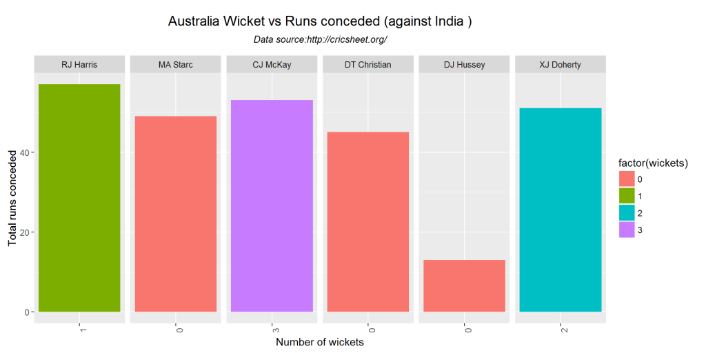
16. Top ODI bowlers wicket runs
The plot below gives the top 8 performances of bowlers against India with wickets taken and runs conceded. The maximum wickets is 44 (pink) and Mitchell Johnson has taken it conceding around 1000 runs. Kulasekara has 40 wickets (purple) conceding around 1400 runs
teamBowlingWicketRunsAllOppn(matches,t1="India",t2="All")
![]()

The plots below give the top 8 Indian bowlers against different countries. The bar that is rightmost is the most wickets and the taller the bar more the runs conceded.
teamBowlingWicketRunsAllOppn(matches,t1="India",t2="Zimbabwe")
![]()

teamBowlingWicketRunsAllOppn(matches,t1="India",t2="Australia")
![]()

teamBowlingWicketRunsAllOppn(matches,t1="India",t2="Pakistan")
![]()

teamBowlingWicketRunsAllOppn(matches,t1="India",t2="New Zealand")
![]()