In this post I use Weights and Biases’ wandb.ai ‘sweep’ feature, to automatically select the best Deep Learning model out of a set of models created through Grid Search. I chanced upon the Weights and Biases site when I was training and fine-tuning the T5 transformer model, on Kaggle, for my post GenerativeAI:Using T5 Transformer model to summarise Indian Philosophy. During this process Kaggle had requested for a token from wandb.ai.
Out of curiosity, I started to explore this Weights and Biases (W&B) machine learning site and was impressed with the visualisation capabilities of this site. So I decided to give weights and biases a try. It is quite interesting to see the live visualisation features of the site and it is becomes very easy to select the optimal model when we are trying to do a Grid search or Random search through a combination of hyper-parameters.
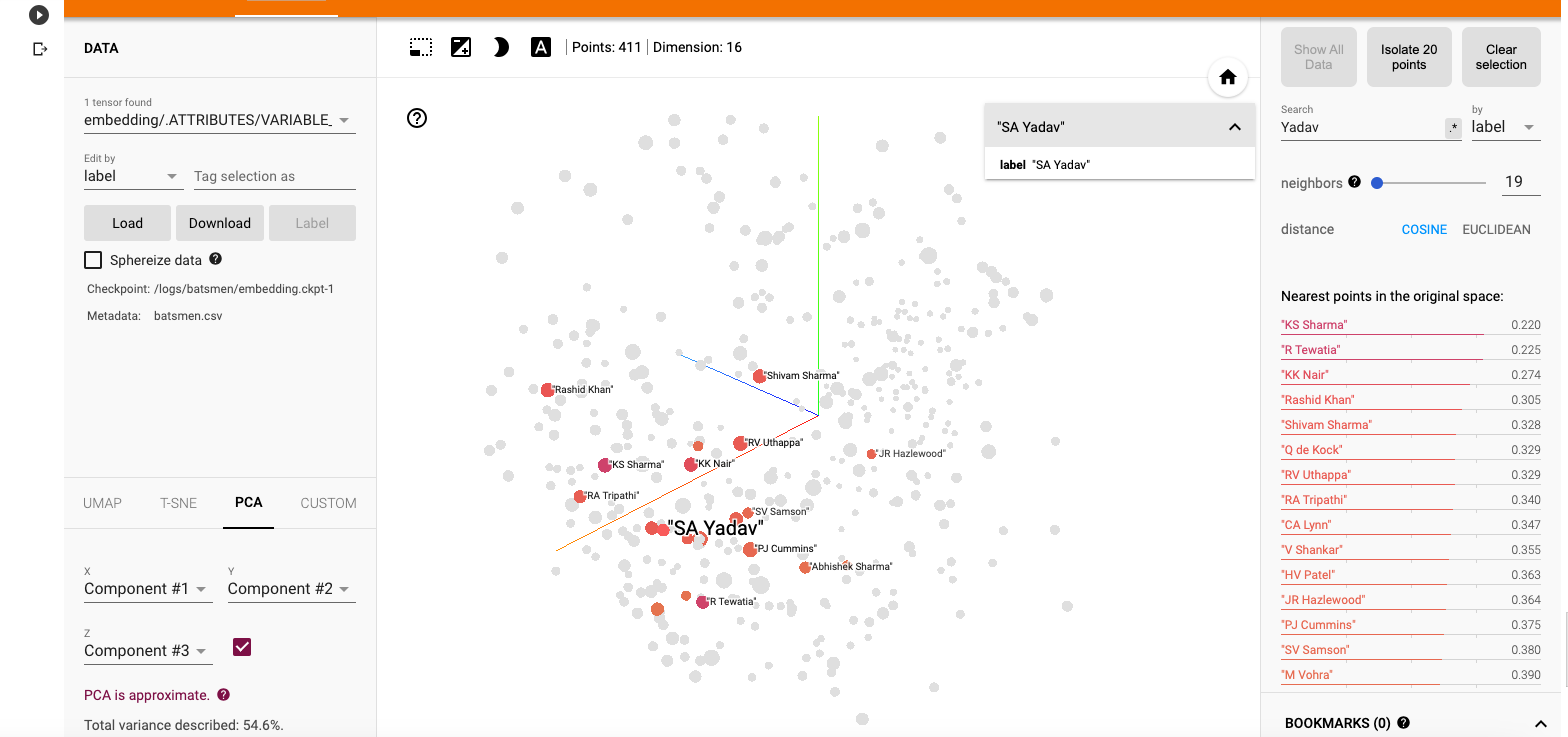
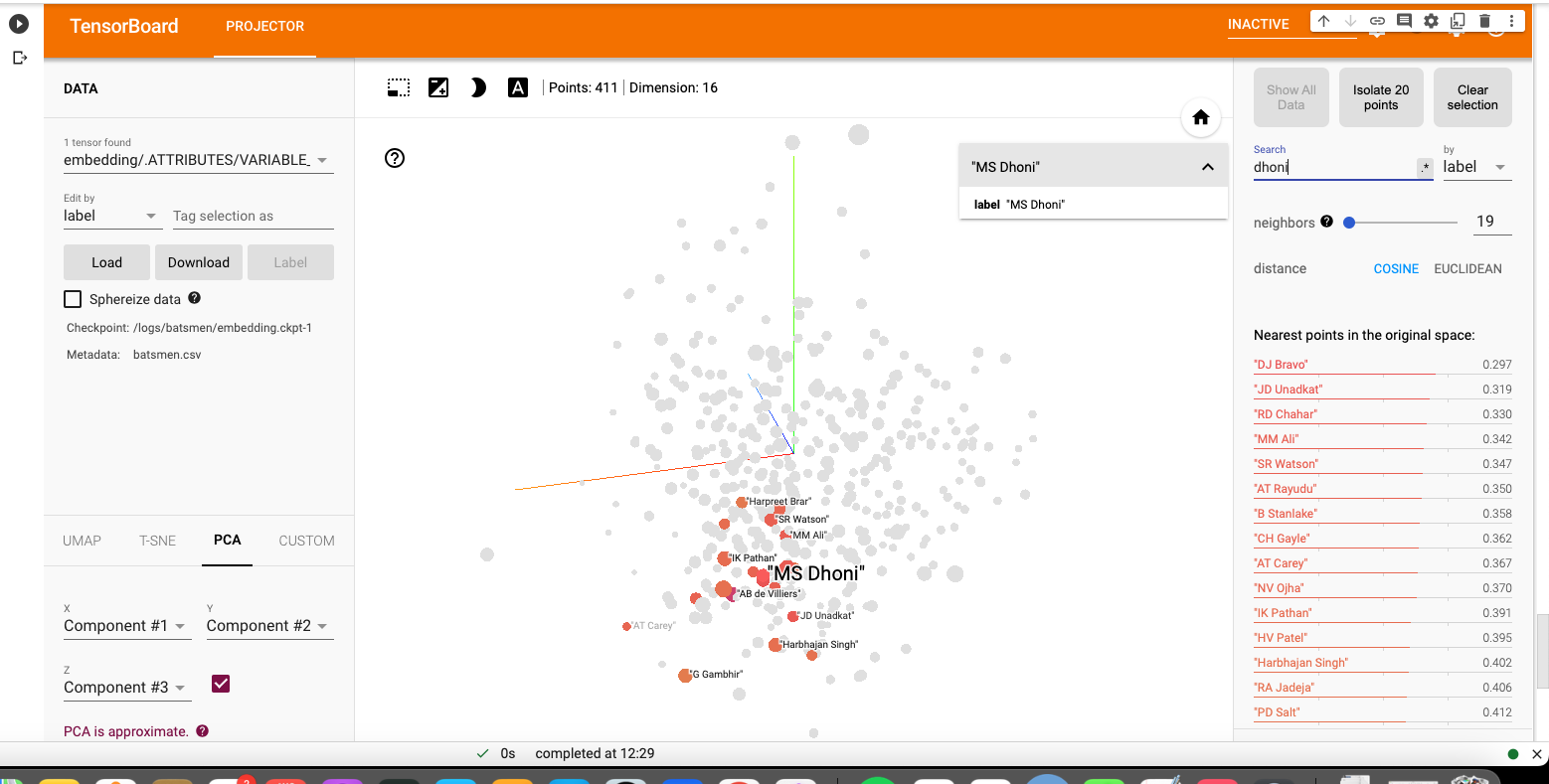
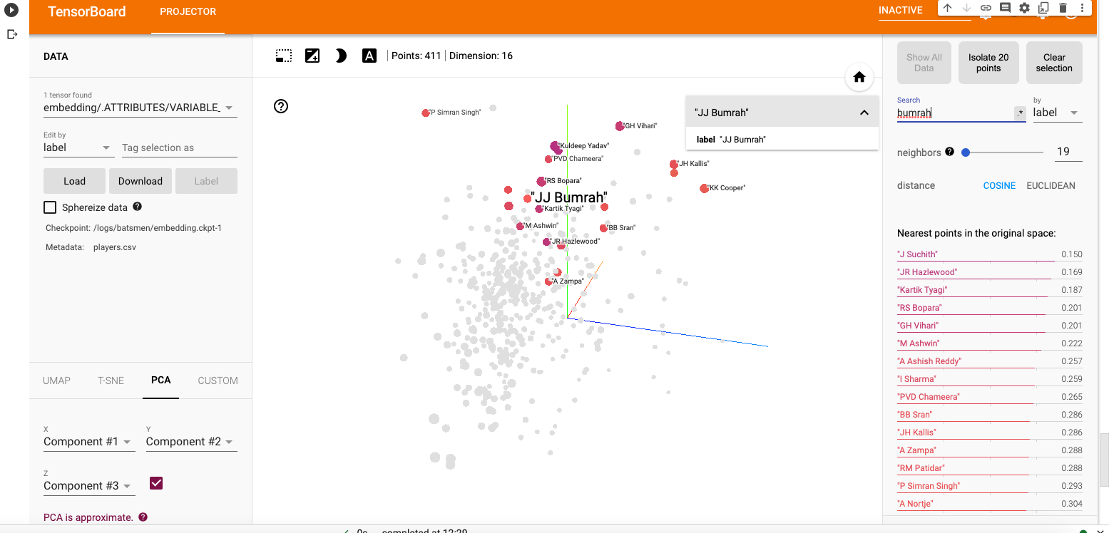
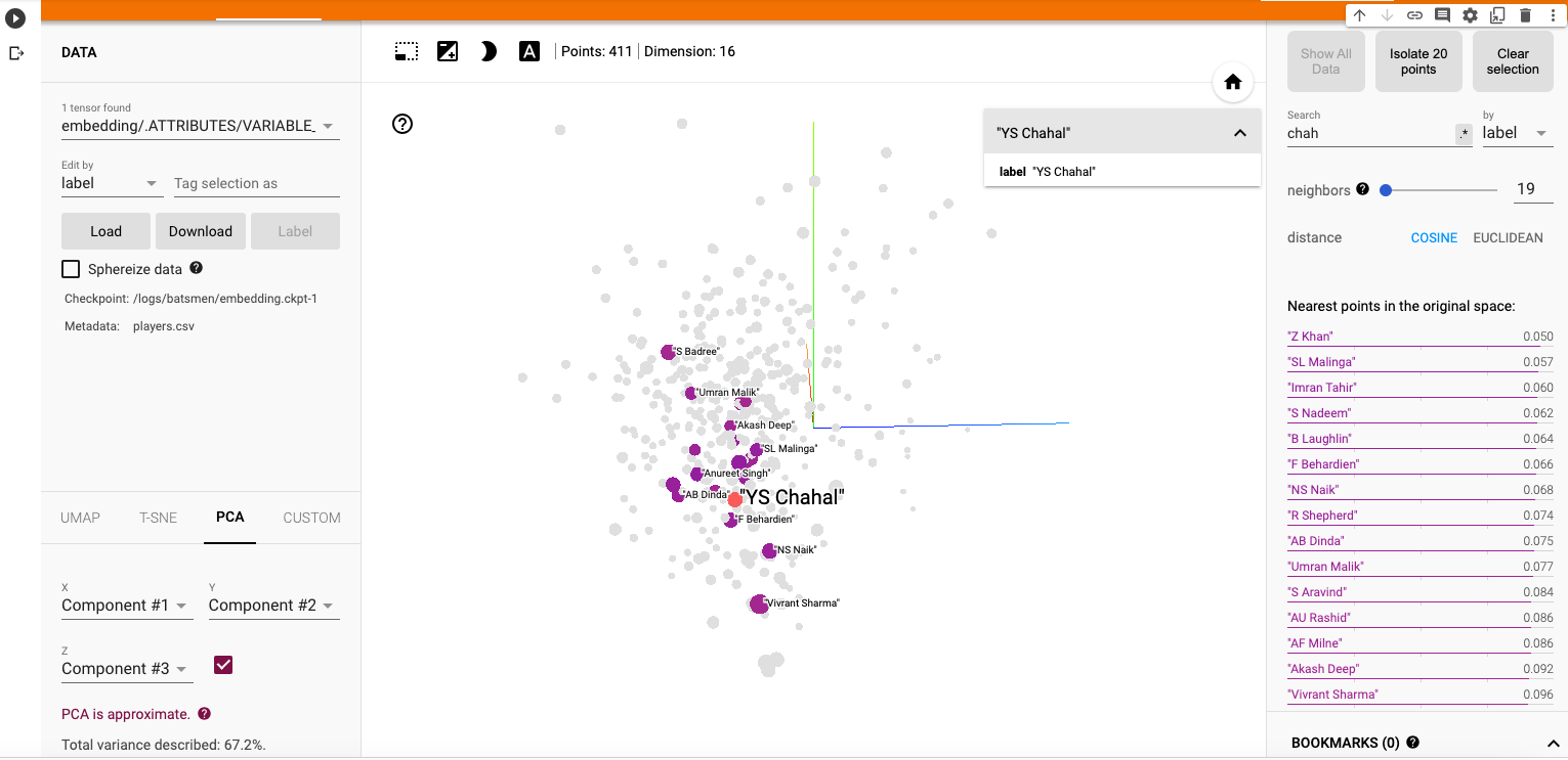
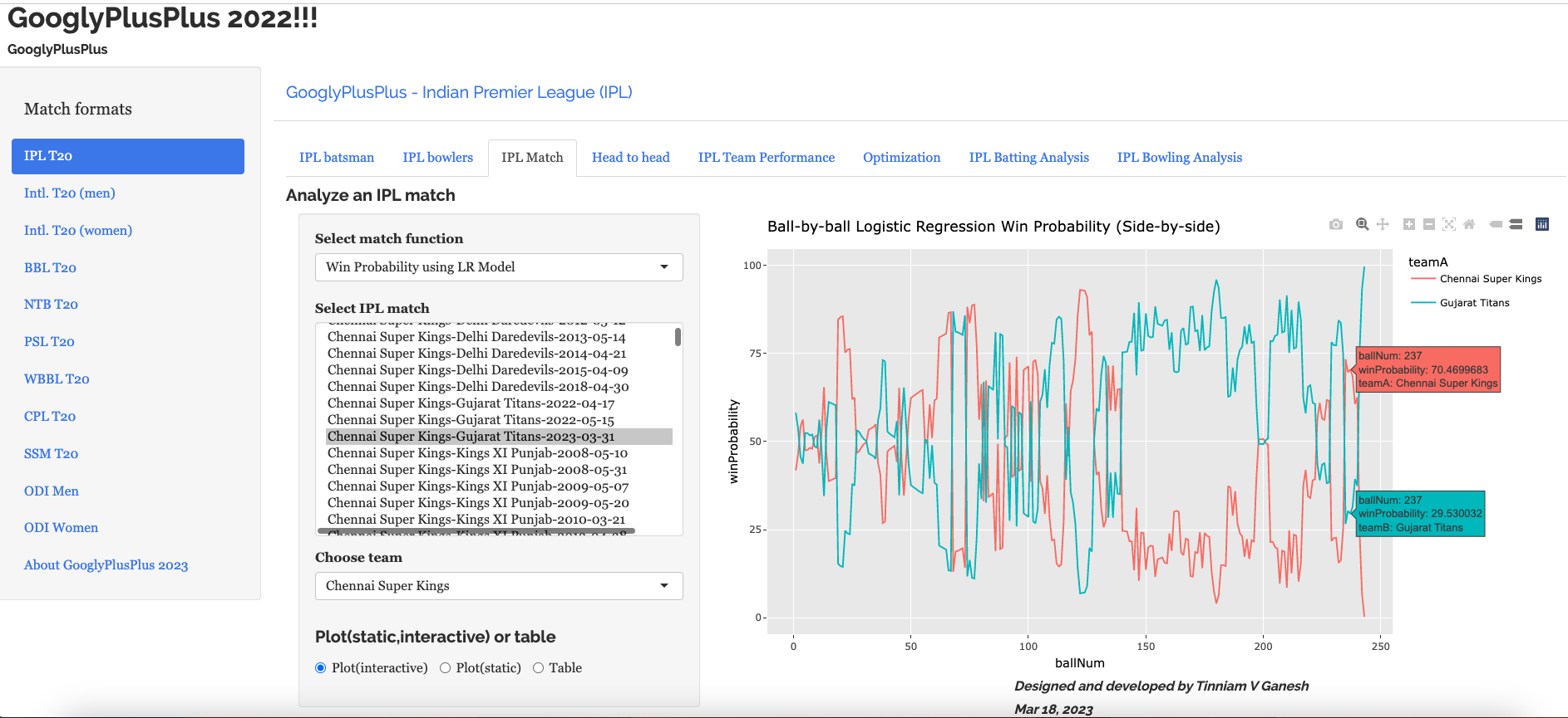
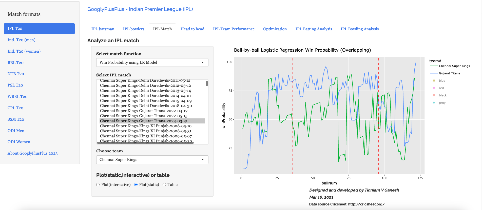
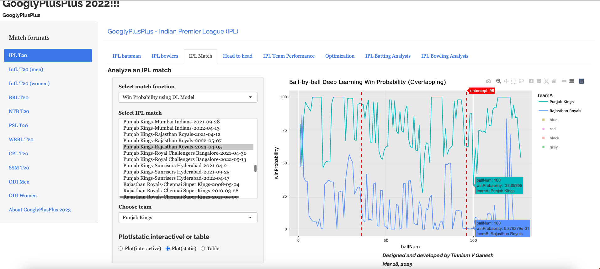
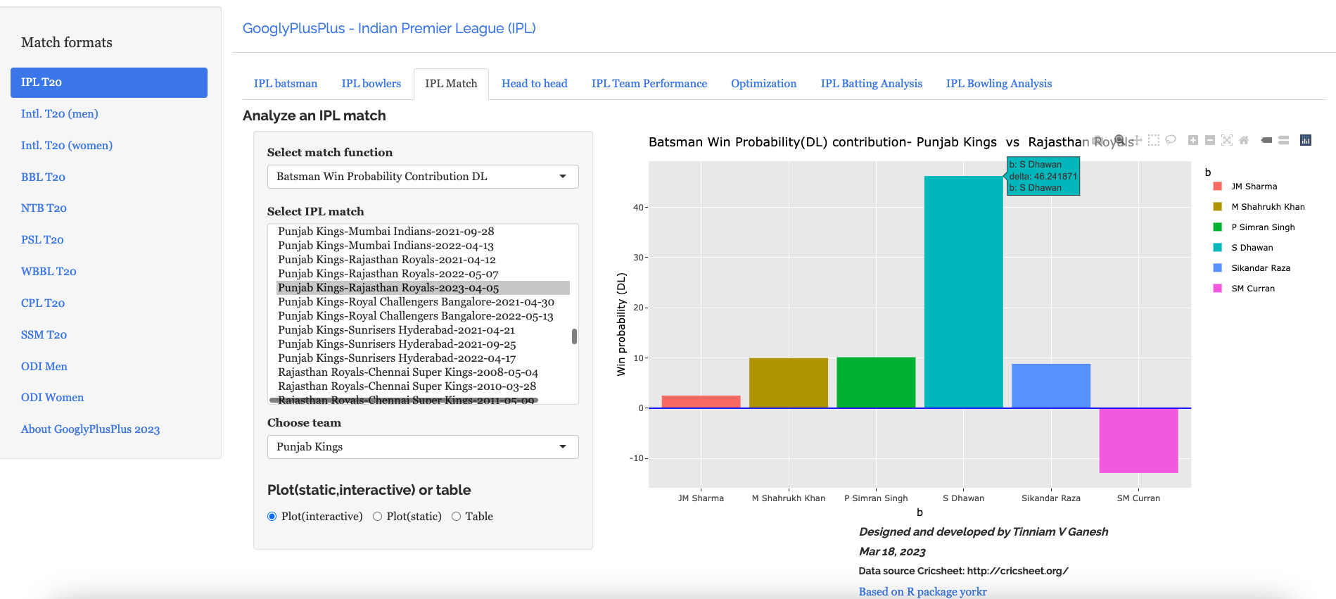
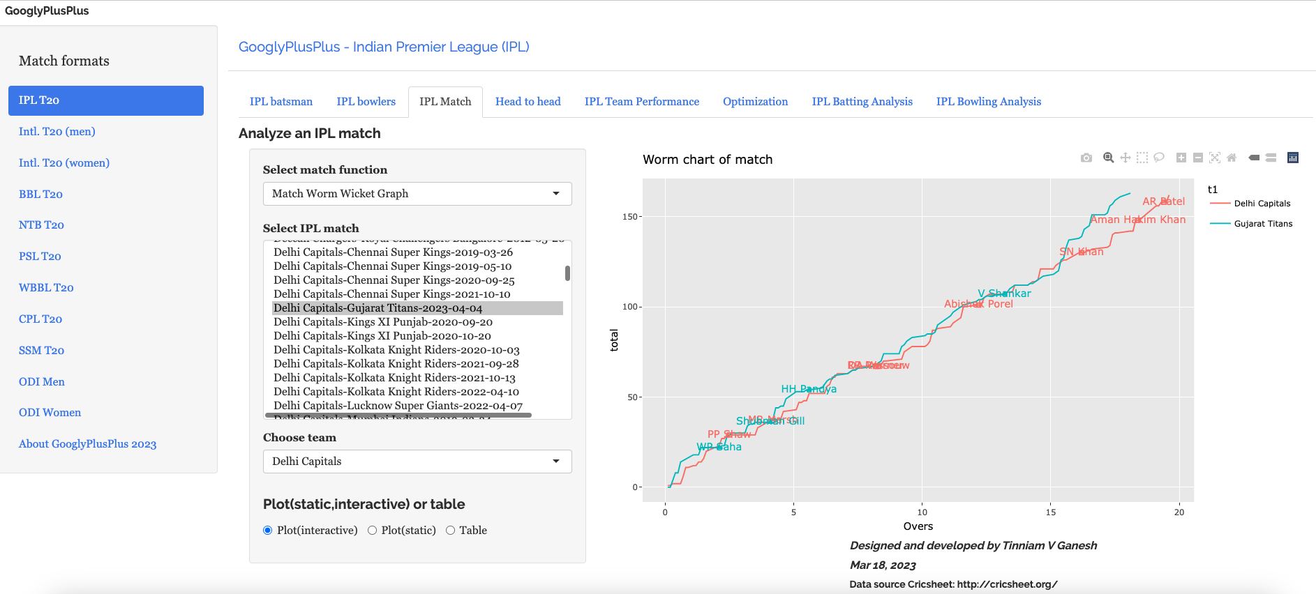
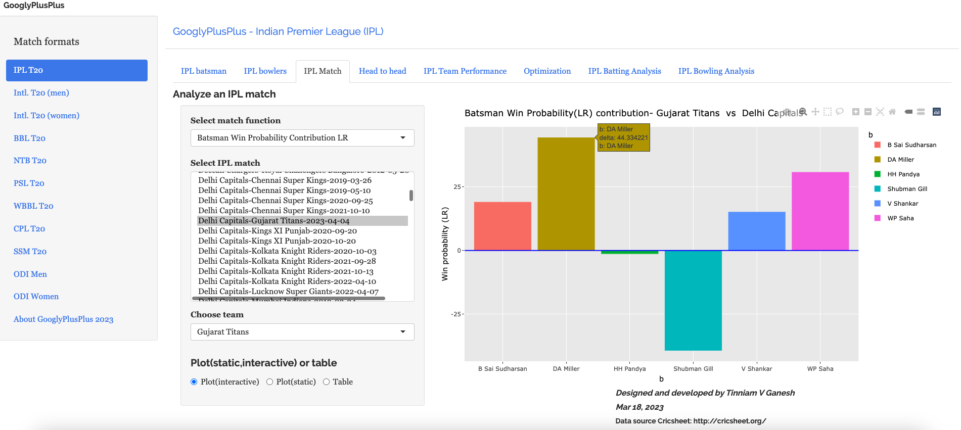
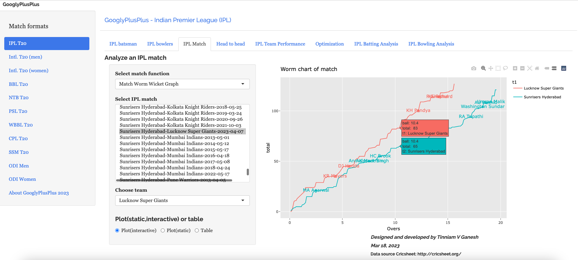
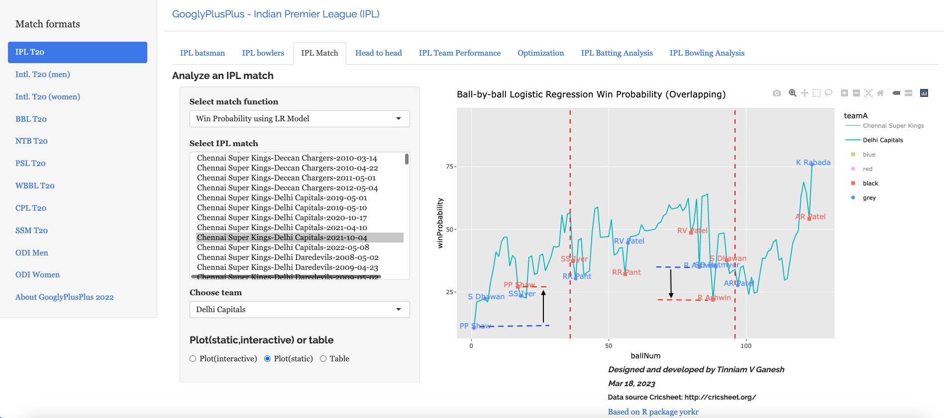
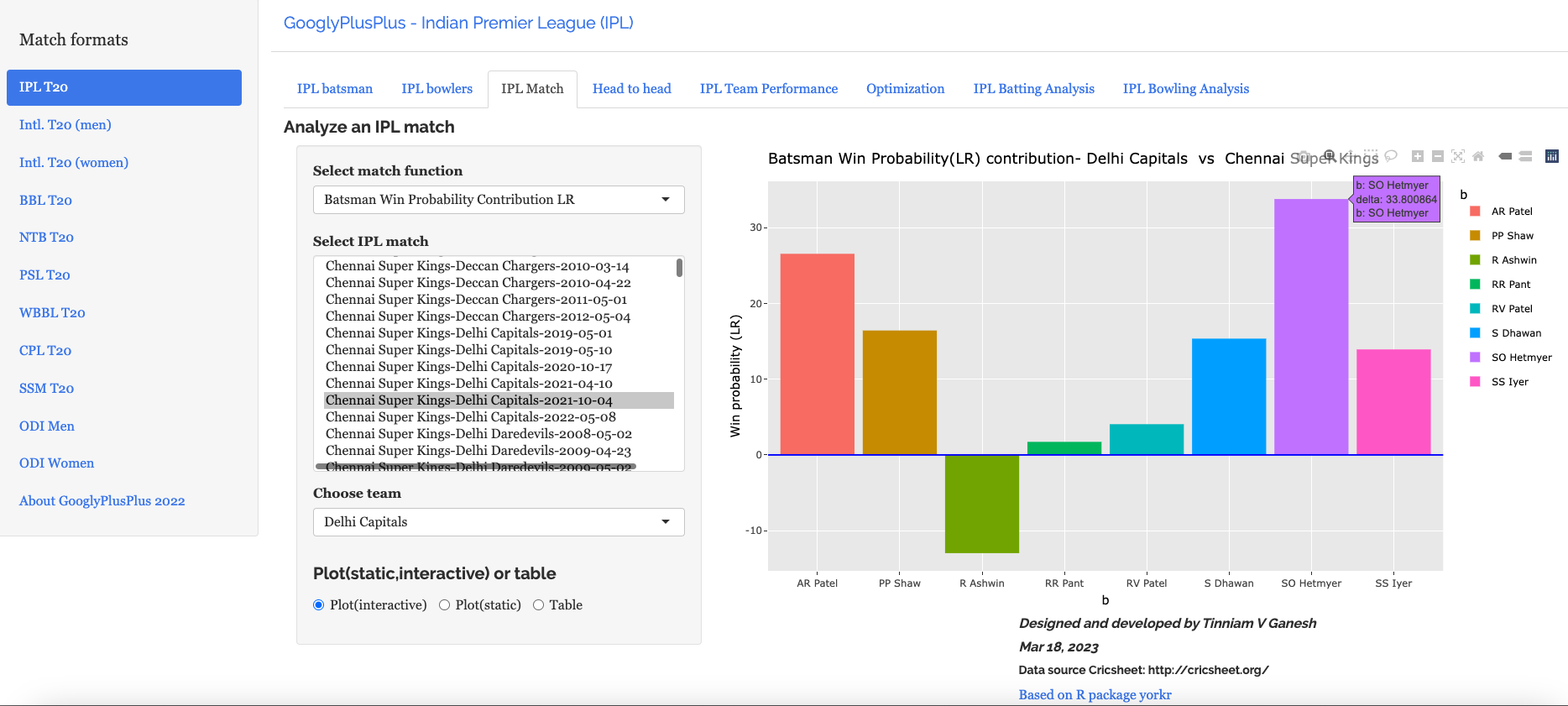
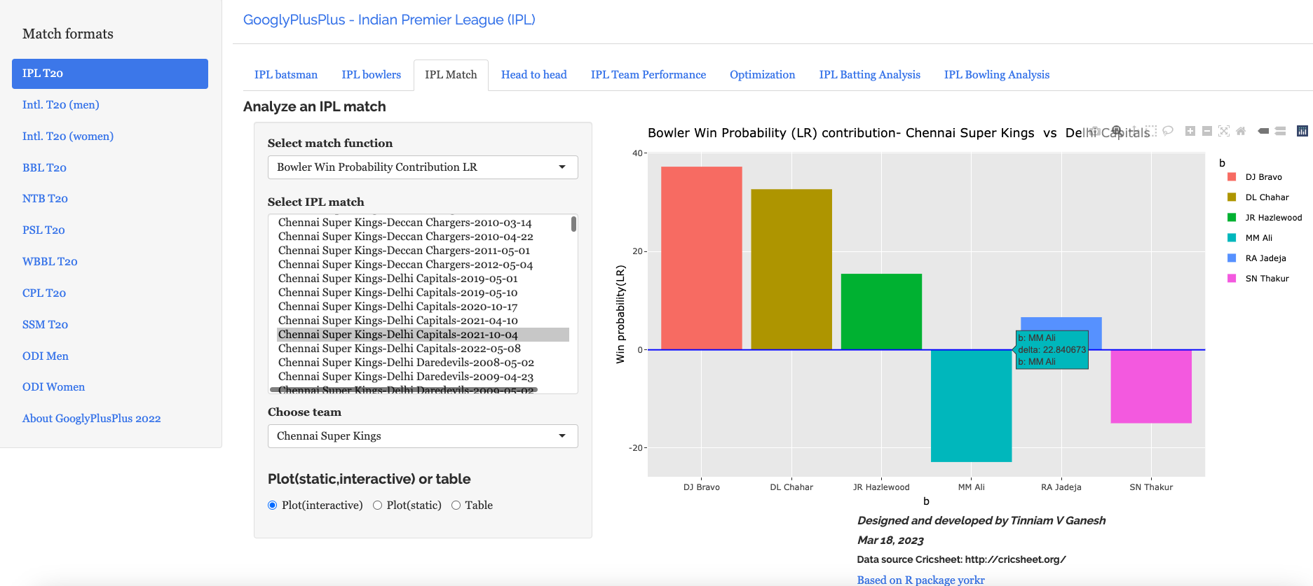
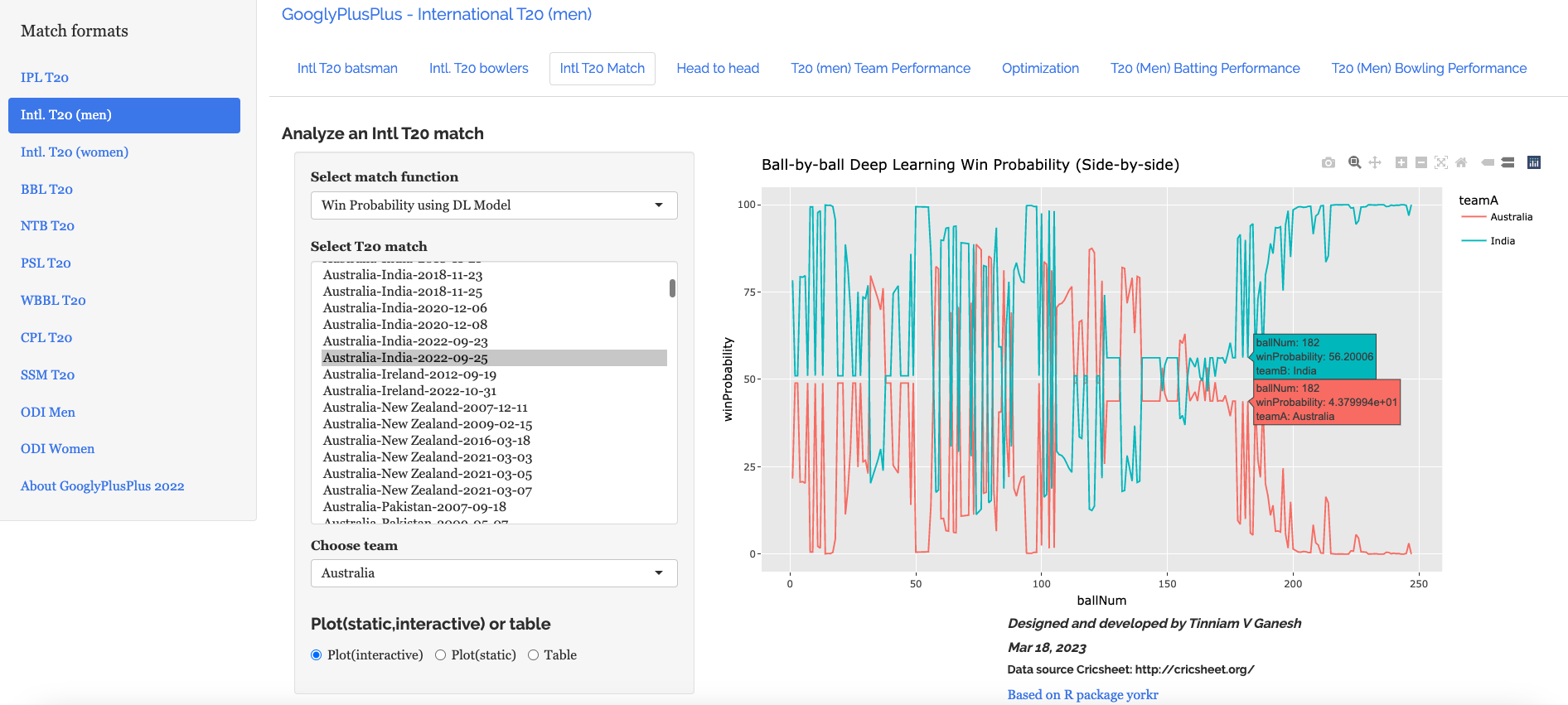
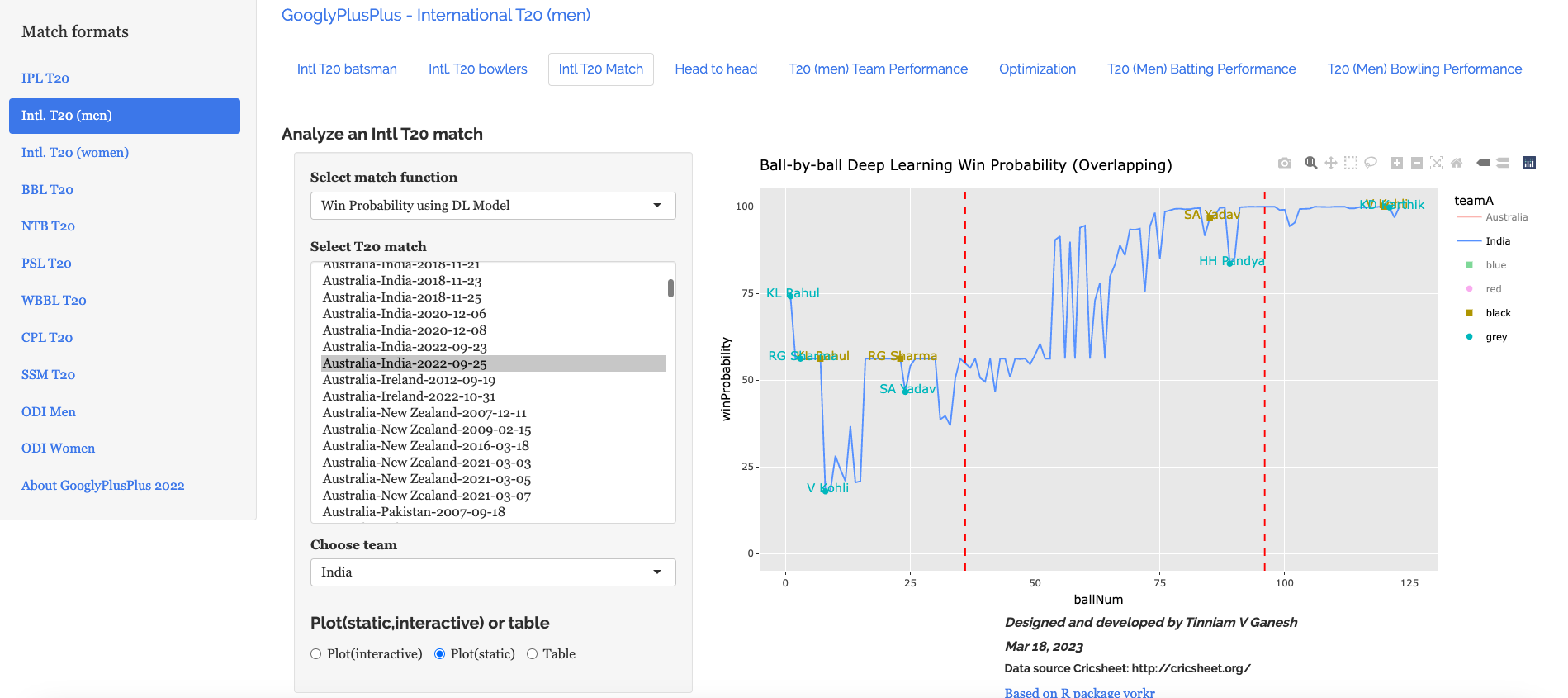
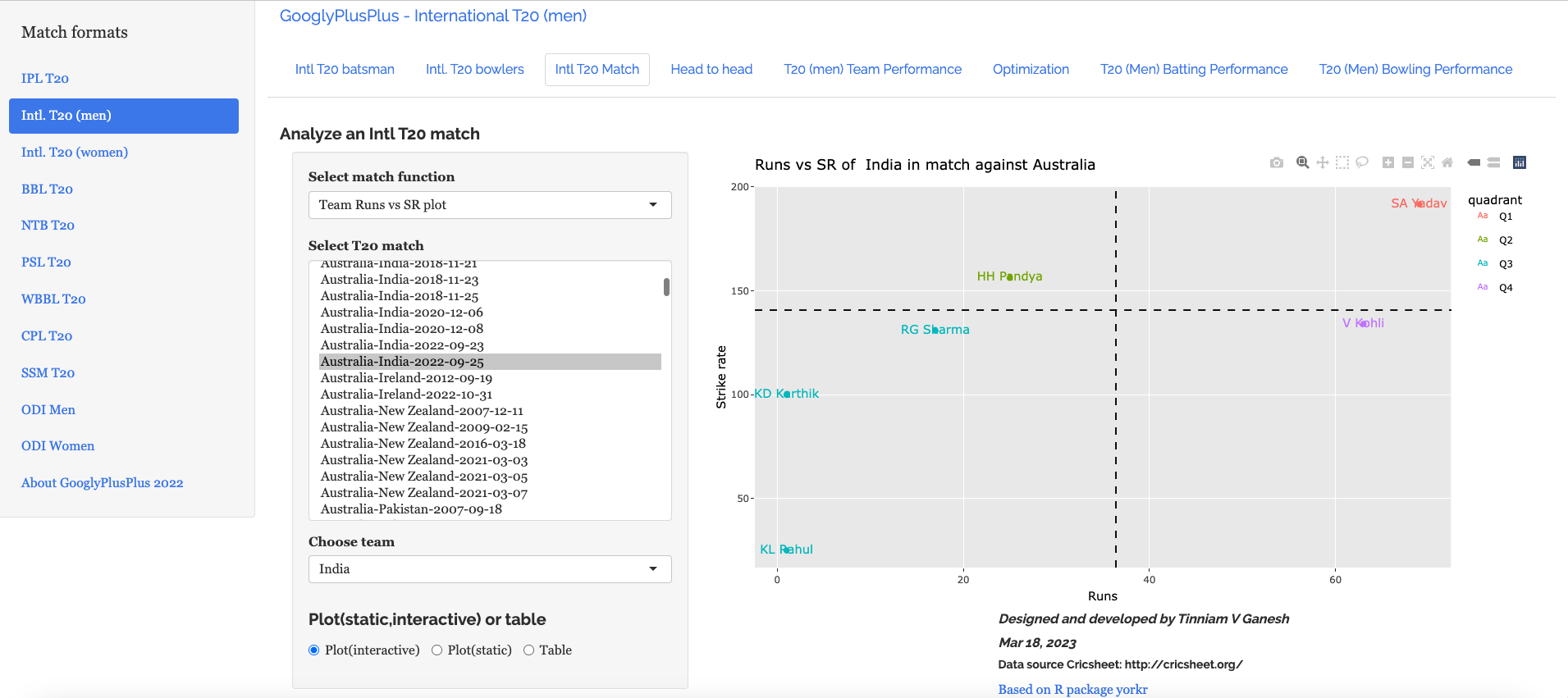
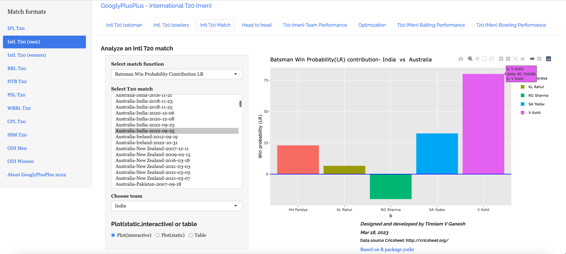
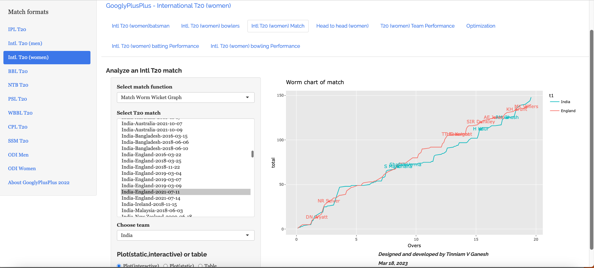
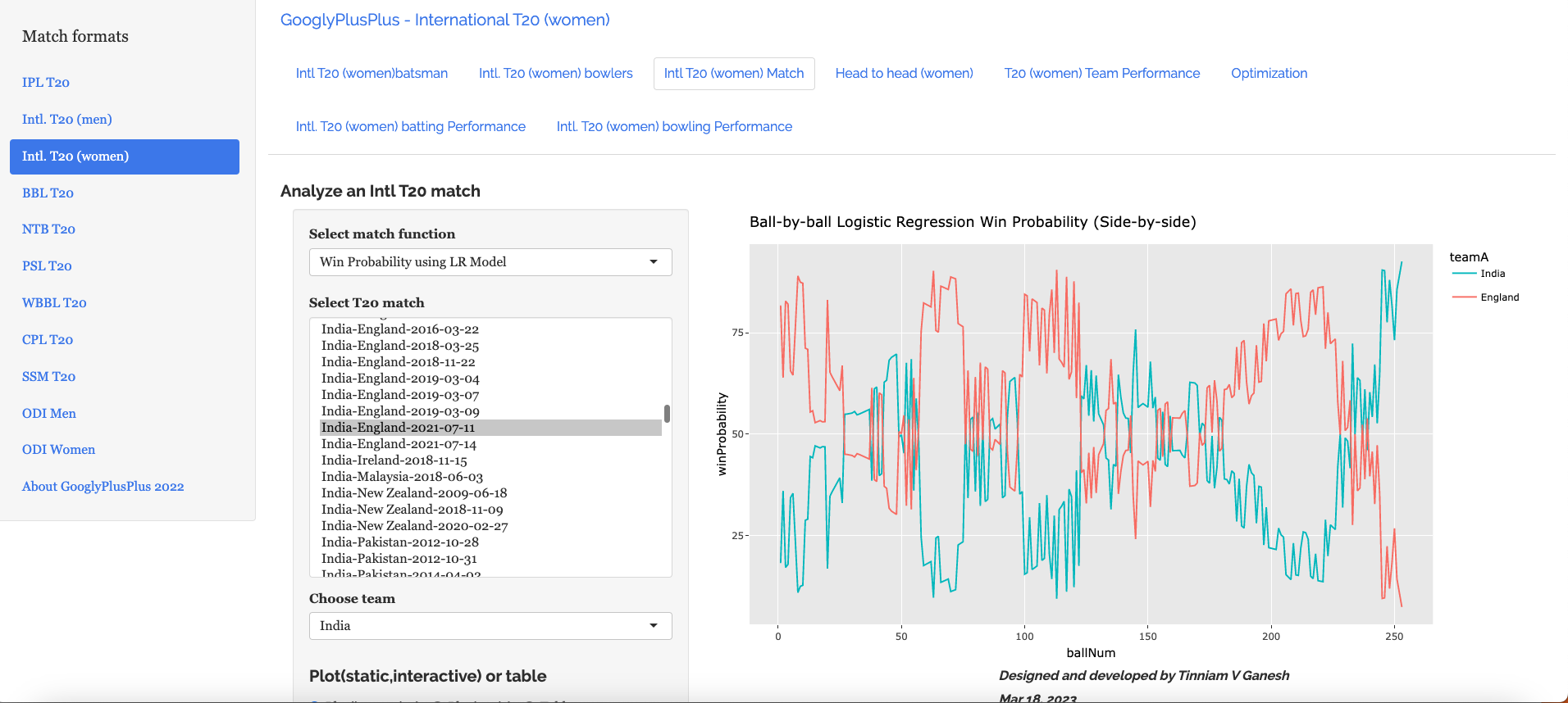
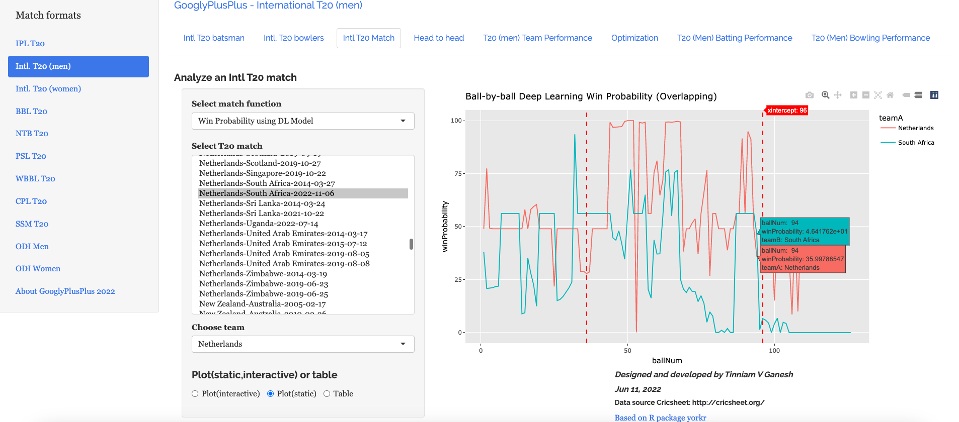
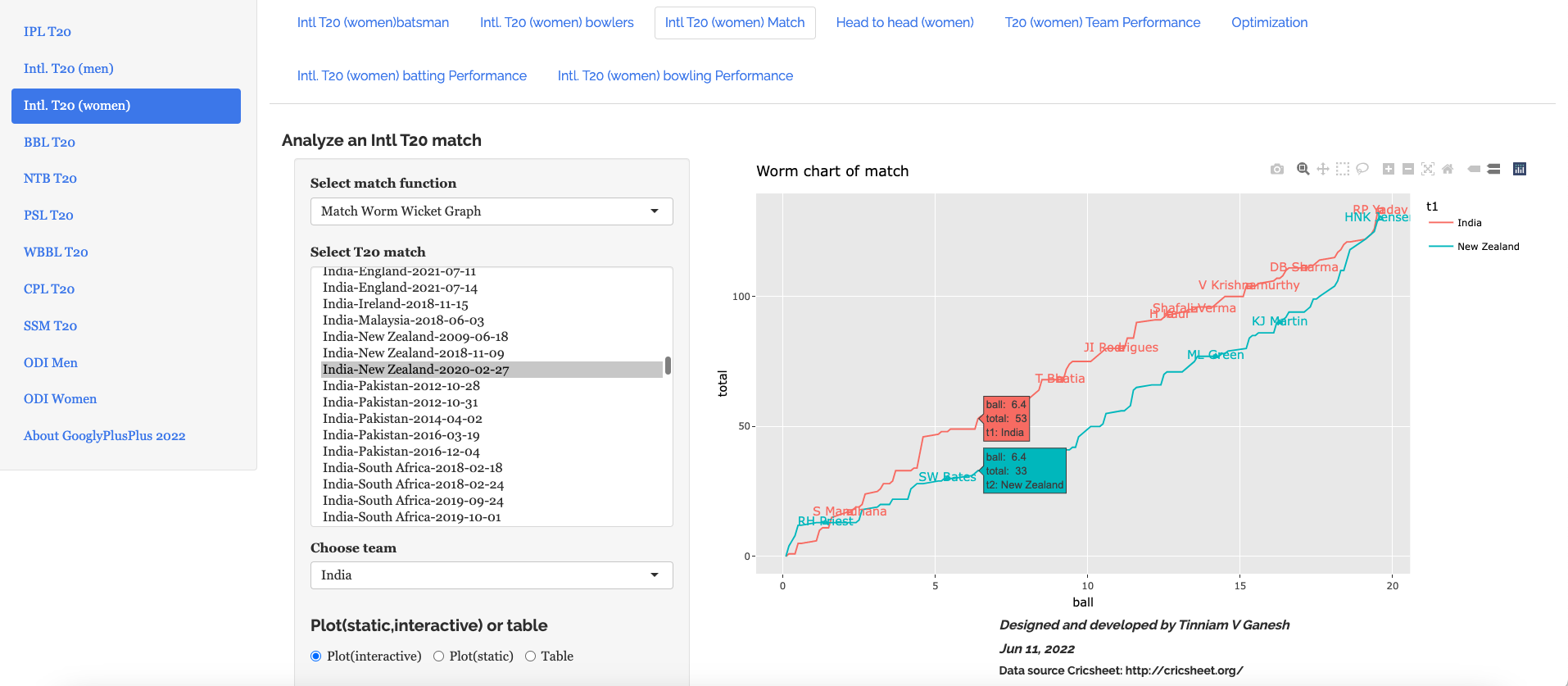
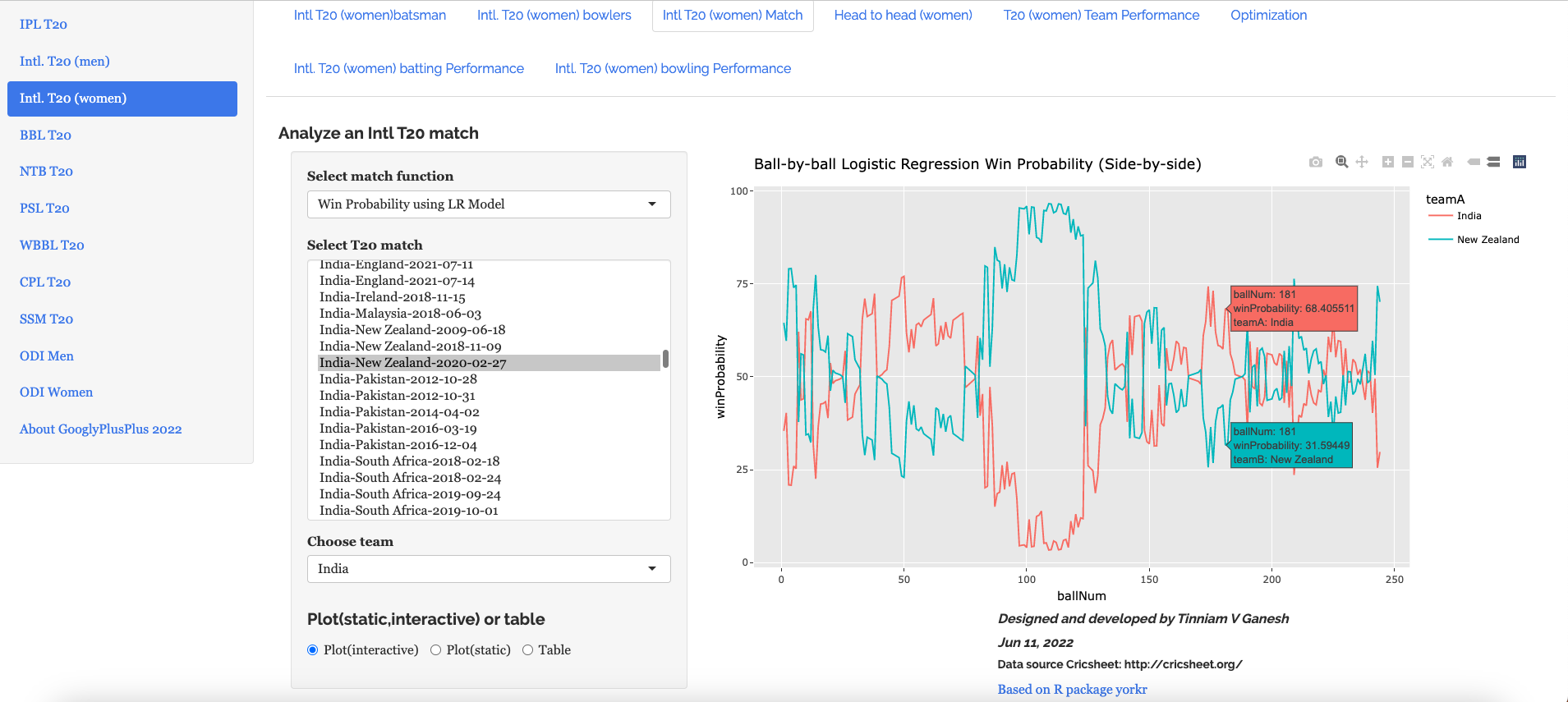
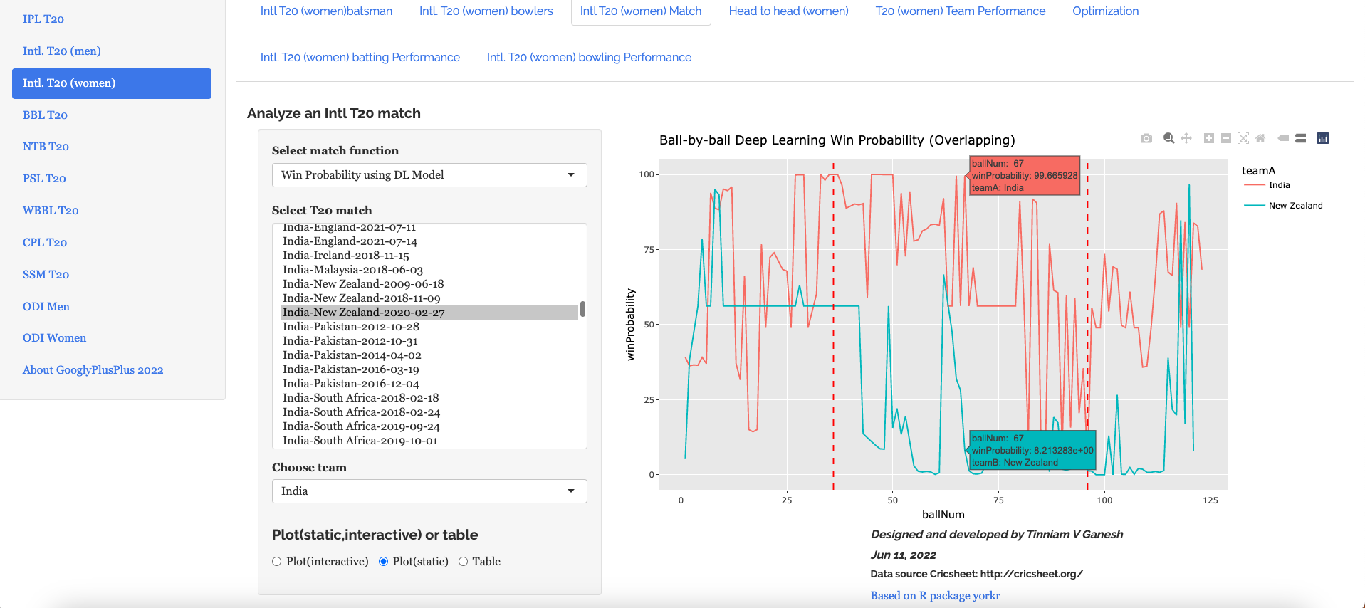
For this purpose, I used my processed T20 match dataset which I had used to compute the Win Probability of T20 teams. For more details please see my post GooglyPlusPlus: Win Probability using Deep Learning and player embeddings
Searching through high dimensional hyperparameter spaces to find the most performant model can quickly get unwieldy. Hyperparameter sweeps provide an organised and efficient way to automatically search through combinations of hyperparameter values (e.g. learning rate, batch size, epochs, dropout, optimizer type) to find the most optimal values.
Here are the steps
a) Install, import
!pip install wandb -qUimport wandb
from wandb.keras import WandbCallback
wandb.login()import pandas as pd
import numpy as np
from zipfile import ZipFile
import tensorflow as tf
from tensorflow import keras
from tensorflow.keras import layers
from tensorflow.keras import regularizers
from pathlib import Path
import matplotlib.pyplot as pltb) Load the dataset
import pandas as pd
import numpy as np
from zipfile import ZipFile
import tensorflow as tf
from tensorflow import keras
from tensorflow.keras import layers
from tensorflow.keras import regularizers

df1=pd.read_csv('t20.csv')
print("Shape of dataframe=",df1.shape)

train_dataset = df1.sample(frac=0.8,random_state=0)
test_dataset = df1.drop(train_dataset.index)
train_dataset1 = train_dataset[['batsmanIdx','bowlerIdx','ballNum','ballsRemaining','runs','runRate','numWickets','runsMomentum','perfIndex']]
test_dataset1 = test_dataset[['batsmanIdx','bowlerIdx','ballNum','ballsRemaining','runs','runRate','numWickets','runsMomentum','perfIndex']]
train_dataset1
train_labels = train_dataset.pop('isWinner')
test_labels = test_dataset.pop('isWinner')
train_dataset1

a=train_dataset1.describe()
stats=a.transpose
a

Shape of dataframe= (1359888, 10)
batsmanIdx	bowlerIdx	ballNum	ballsRemaining	runs	runRate	numWickets	runsMomentum	perfIndex
count	1.087910e+06	1.087910e+06	1.087910e+06	1.087910e+06	1.087910e+06	1.087910e+06	1.087910e+06	1.087910e+06	1.087910e+06
mean	2.561058e+03	1.939449e+03	1.185352e+02	6.001942e+01	8.110290e+01	1.611611e+00	2.604912e+00	2.886850e-01	9.619675e+00
std	1.479446e+03	1.095097e+03	6.934078e+01	3.514725e+01	4.977998e+01	2.983874e+00	2.195410e+00	6.066070e-01	4.602859e+00
min	1.000000e+00	1.000000e+00	1.000000e+00	1.000000e+00	-5.000000e+00	-5.000000e+00	0.000000e+00	3.571429e-02	0.000000e+00
25%	1.230000e+03	9.400000e+02	5.900000e+01	3.000000e+01	4.100000e+01	1.043478e+00	1.000000e+00	1.058824e-01	6.539326e+00
50%	2.492000e+03	1.919000e+03	1.170000e+02	5.900000e+01	7.800000e+01	1.300000e+00	2.000000e+00	1.408451e-01	9.246753e+00
75%	3.868000e+03	2.884000e+03	1.770000e+02	9.000000e+01	1.170000e+02	1.590312e+00	4.000000e+00	2.352941e-01	1.218349e+01
max	5.226000e+03	3.848000e+03	2.860000e+02	1.610000e+02	2.780000e+02	2.510000e+02	1.000000e+01	1.100000e+01	6.600000e+01
c) Define the Deep Learning model
import pandas as pd
import numpy as np
from keras.layers import Input, Embedding, Flatten, Dense
from keras.models import Model
from keras.layers import Input, Embedding, Flatten, Dense, Reshape, Concatenate, Dropout
from keras.models import Model

tf.random.set_seed(432)
# create input layers for each of the predictors
batsmanIdx_input = Input(shape=(1,), name='batsmanIdx')
bowlerIdx_input = Input(shape=(1,), name='bowlerIdx')
ballNum_input = Input(shape=(1,), name='ballNum')
ballsRemaining_input = Input(shape=(1,), name='ballsRemaining')
runs_input = Input(shape=(1,), name='runs')
runRate_input = Input(shape=(1,), name='runRate')
numWickets_input = Input(shape=(1,), name='numWickets')
runsMomentum_input = Input(shape=(1,), name='runsMomentum')
perfIndex_input = Input(shape=(1,), name='perfIndex')

# Set the embedding size
no_of_unique_batman=len(df1["batsmanIdx"].unique())
print(no_of_unique_batman)
no_of_unique_bowler=len(df1["bowlerIdx"].unique())
print(no_of_unique_bowler)
embedding_size_bat = no_of_unique_batman ** (1/4)
embedding_size_bwl = no_of_unique_bowler ** (1/4)


# create embedding layer for the categorical predictor
batsmanIdx_embedding = Embedding(input_dim=no_of_unique_batman+1, output_dim=16,input_length=1)(batsmanIdx_input)
batsmanIdx_flatten = Flatten()(batsmanIdx_embedding)
bowlerIdx_embedding = Embedding(input_dim=no_of_unique_bowler+1, output_dim=16,input_length=1)(bowlerIdx_input)
bowlerIdx_flatten = Flatten()(bowlerIdx_embedding)

# concatenate all the predictors
x = keras.layers.concatenate([batsmanIdx_flatten,bowlerIdx_flatten, ballNum_input, ballsRemaining_input, runs_input, runRate_input, numWickets_input, runsMomentum_input, perfIndex_input])

# add hidden layers
x = Dense(64, activation='relu')(x)
x = Dropout(0.1)(x)
x = Dense(32, activation='relu')(x)
x = Dropout(0.1)(x)
x = Dense(16, activation='relu')(x)
x = Dropout(0.1)(x)
x = Dense(8, activation='relu')(x)
x = Dropout(0.1)(x)
# add output layer
output = Dense(1, activation='sigmoid', name='output')(x)
print(output.shape)
# create model

# Initialize a new W&B run
#run = wandb.init(project='t20', group='cricket')

model = Model(inputs=[batsmanIdx_input,bowlerIdx_input, ballNum_input, ballsRemaining_input, runs_input, runRate_input, numWickets_input, runsMomentum_input, perfIndex_input], outputs=output)
model.summary()

# Initialize a new W&B run
run = wandb.init(project='t20', group='cricket')
wandb.init(
    # set the wandb project where this run will be logged
    project="t20",

    # track hyperparameters and run metadata
    config={
    "learning_rate": 0.02,
    "dropout": 0.01,
    "batch_size": 1024,
    "epochs": 5,
    }
)


5226
3848
(None, 1)
Model: "model"
__________________________________________________________________________________________________
 Layer (type)                Output Shape                 Param #   Connected to
==================================================================================================
 batsmanIdx (InputLayer)     [(None, 1)]                  0         []

 bowlerIdx (InputLayer)      [(None, 1)]                  0         []

 embedding (Embedding)       (None, 1, 16)                83632     ['batsmanIdx[0][0]']

 embedding_1 (Embedding)     (None, 1, 16)                61584     ['bowlerIdx[0][0]']

 flatten (Flatten)           (None, 16)                   0         ['embedding[0][0]']

 flatten_1 (Flatten)         (None, 16)                   0         ['embedding_1[0][0]']

 ballNum (InputLayer)        [(None, 1)]                  0         []

 ballsRemaining (InputLayer  [(None, 1)]                  0         []
 )

 runs (InputLayer)           [(None, 1)]                  0         []

 runRate (InputLayer)        [(None, 1)]                  0         []

 numWickets (InputLayer)     [(None, 1)]                  0         []

 runsMomentum (InputLayer)   [(None, 1)]                  0         []

 perfIndex (InputLayer)      [(None, 1)]                  0         []

 concatenate (Concatenate)   (None, 39)                   0         ['flatten[0][0]',
                                                                     'flatten_1[0][0]',
                                                                     'ballNum[0][0]',
                                                                     'ballsRemaining[0][0]',
                                                                     'runs[0][0]',
                                                                     'runRate[0][0]',
                                                                     'numWickets[0][0]',
                                                                     'runsMomentum[0][0]',
                                                                     'perfIndex[0][0]']

 dense (Dense)               (None, 64)                   2560      ['concatenate[0][0]']

 dropout (Dropout)           (None, 64)                   0         ['dense[0][0]']

 dense_1 (Dense)             (None, 32)                   2080      ['dropout[0][0]']

 dropout_1 (Dropout)         (None, 32)                   0         ['dense_1[0][0]']

 dense_2 (Dense)             (None, 16)                   528       ['dropout_1[0][0]']

 dropout_2 (Dropout)         (None, 16)                   0         ['dense_2[0][0]']

 dense_3 (Dense)             (None, 8)                    136       ['dropout_2[0][0]']

 dropout_3 (Dropout)         (None, 8)                    0         ['dense_3[0][0]']

 output (Dense)              (None, 1)                    9         ['dropout_3[0][0]']

==================================================================================================
Total params: 150529 (588.00 KB)
Trainable params: 150529 (588.00 KB)
Non-trainable params: 0 (0.00 Byte)
d) Create a Training script
def get_optimizer(lr=1e-2, optimizer="adam"):
    "Select optmizer between adam and sgd with momentum"
    if optimizer.lower() == "adam":
        return tf.keras.optimizers.Adam(learning_rate=lr)
    if optimizer.lower() == "sgd":
        return tf.keras.optimizers.SGD(learning_rate=lr, momentum=0.1)

def train(model, batch_size=1024, epochs=10, lr=1e-2, optimizer='adam', log_freq=10):

    # Compile model like you usually do.
    tf.keras.backend.clear_session()
    model.compile(loss="binary_crossentropy",
                  optimizer=get_optimizer(lr, optimizer),
                  metrics=["accuracy"])

    # callback setup
    cbs = [WandbCallback(data_type='auto', log_batch_frequency=None)]

    # train the model
    history=model.fit([train_dataset1['batsmanIdx'],train_dataset1['bowlerIdx'],train_dataset1['ballNum'],train_dataset1['ballsRemaining'],train_dataset1['runs'],
           train_dataset1['runRate'],train_dataset1['numWickets'],train_dataset1['runsMomentum'],train_dataset1['perfIndex']], train_labels, epochs=epochs, batch_size=batch_size,callbacks=cbs,
          validation_data = ([test_dataset1['batsmanIdx'],test_dataset1['bowlerIdx'],test_dataset1['ballNum'],test_dataset1['ballsRemaining'],test_dataset1['runs'],
           test_dataset1['runRate'],test_dataset1['numWickets'],test_dataset1['runsMomentum'],test_dataset1['perfIndex']],test_labels), verbose=1)
e) Define the sweep for Grid Search
#Grid search
sweep_config = {
    'method': 'grid'
    }

metric = {
    'name': 'val_loss',
    'goal': 'minimize'
    }

sweep_config['metric'] = metric
# Optimizers - Adam, SGD
parameters_dict = {
    'optimizer': {
        'values': ['adam', 'sgd']
        },
    'dropout': {
          'values': [0.1, 0.05]
        },
    }

sweep_config['parameters'] = parameters_dict

parameters_dict.update({
    'epochs': {
        'value': 20}
    })

import math
# Set learning_rate, batch_size
parameters_dict.update({
    'learning_rate': {
         'values': [0.005,0.008,0.01,.03]
      },
    'batch_size': {
        'values': [1024,2048]
      }
    })
import pprint
pprint.pprint(sweep_config)

'method': 'grid',
 'metric': {'goal': 'minimize', 'name': 'val_loss'},
 'parameters': {'batch_size': {'values': [1024, 2048]},
                'dropout': {'values': [0.1, 0.05]},
                'epochs': {'value': 20},
                'learning_rate': {'values': [0.005, 0.008, 0.01, 0.03]},
                'optimizer': {'values': ['adam', 'sgd']}}}
f) Wrap the Training Loop
def sweep_train(config_defaults=None):
    # Initialize wandb with a sample project name
    with wandb.init(config=config_defaults):  # this gets over-written in the Sweep

        # Specify the other hyperparameters to the configuration, if any
        wandb.config.architecture_name = "DL"
        wandb.config.dataset_name = "T20"
        # initialize model
        #model = T20Net(wandb.config.dropout)

        train(model,
              wandb.config.batch_size,
              wandb.config.epochs,
              wandb.config.learning_rate,
              wandb.config.optimizer)
g) Initialise Sweep and Run Agent
sweep_id = wandb.sweep(sweep_config, project="sweeps-keras-t20")wandb.agent(sweep_id, sweep_train, count=10)wandb: WARNING Calling wandb.login() after wandb.init() has no effect.
wandb: Agent Starting Run: zbaaq0bn with config:
wandb: batch_size: 1024
wandb: dropout: 0.1
wandb: epochs: 20
wandb: learning_rate: 0.005
wandb: optimizer: adam
Epoch 19/20
1061/1063 [============================>.] - ETA: 0s - loss: 0.3073 - accuracy: 0.8490/usr/local/lib/python3.10/dist-packages/keras/src/engine/training.py:3000: UserWarning: You are saving your model as an HDF5 file via `model.save()`. This file format is considered legacy. We recommend using instead the native Keras format, e.g. `model.save('my_model.keras')`.
saving_api.save_model(
wandb: Adding directory to artifact (/content/wandb/run-20231004_065327-zbaaq0bn/files/model-best)... Done. 0.0s
1063/1063 [==============================] - 15s 14ms/step - loss: 0.3073 - accuracy: 0.8490 - val_loss: 0.3093 - val_accuracy: 0.8479
Epoch 20/20
1062/1063 [============================>.] - ETA: 0s - loss: 0.3052 - accuracy: 0.8502/usr/local/lib/python3.10/dist-packages/keras/src/engine/training.py:3000: UserWarning: You are saving your model as an HDF5 file via `model.save()`. This file format is considered legacy. We recommend using instead the native Keras format, e.g. `model.save('my_model.keras')`.
saving_api.save_model(
wandb: Adding directory to artifact (/content/wandb/run-20231004_065327-zbaaq0bn/files/model-best)... Done. 0.0s
1063/1063 [==============================] - 18s 17ms/step - loss: 0.3052 - accuracy: 0.8502 - val_loss: 0.3068 - val_accuracy: 0.8490
Waiting for W&B process to finish... (success).
Run history:
accuracy ▁▅▅▆▆▆▇▇▇▇▇▇▇███████
epoch ▁▁▂▂▂▃▃▄▄▄▅▅▅▆▆▇▇▇██
loss █▅▄▃▃▃▃▂▂▂▂▂▂▂▁▁▁▁▁▁
val_accuracy ▁▂▃▄▄▅▅▅▆▆▆▇▇▇▇▇▇███
val_loss █▆▅▅▄▄▃▃▃▃▃▂▂▂▂▂▂▁▁▁
Run summary:
accuracy 0.85022
best_epoch 19
best_val_loss 0.30681
epoch 19
loss 0.30521
val_accuracy 0.849
val_loss 0.30681
...
...
wandb: Agent Starting Run: 4qtyxzq9 with config:
wandb: batch_size: 1024
wandb: dropout: 0.1
wandb: epochs: 20
wandb: learning_rate: 0.008
wandb: optimizer: sgd
...
...
Epoch 18/20
1063/1063 [==============================] - 13s 12ms/step - loss: 0.2672 - accuracy: 0.8697 - val_loss: 0.2819 - val_accuracy: 0.8624
Epoch 19/20
1061/1063 [============================>.] - ETA: 0s - loss: 0.2669 - accuracy: 0.8697/usr/local/lib/python3.10/dist-packages/keras/src/engine/training.py:3000: UserWarning: You are saving your model as an HDF5 file via `model.save()`. This file format is considered legacy. We recommend using instead the native Keras format, e.g. `model.save('my_model.keras')`.
saving_api.save_model(
wandb: Adding directory to artifact (/content/wandb/run-20231004_070920-4qtyxzq9/files/model-best)... Done. 0.0s
1063/1063 [==============================] - 14s 13ms/step - loss: 0.2669 - accuracy: 0.8697 - val_loss: 0.2813 - val_accuracy: 0.8635
Epoch 20/20
1063/1063 [==============================] - 13s 12ms/step - loss: 0.2650 - accuracy: 0.8707 - val_loss: 0.2957 - val_accuracy: 0.8557
Waiting for W&B process to finish... (success).
6.805 MB of 6.818 MB uploaded (0.108 MB deduped)
Run history:
accuracy ▁▂▃▃▄▄▄▄▄▄▄▄▅▅▄▆▅▆▆█
epoch ▁▁▂▂▂▃▃▄▄▄▅▅▅▆▆▇▇▇██
loss █▇▆▆▅▅▅▅▅▅▅▄▄▄▄▄▄▃▃▁
val_accuracy ▇▅▅▁█▅▇▆▆▅█▅▅▆▃▇▁▇█▁
val_loss ▃▄▄▅▁▃▂▃▃▃▁▄▄▂▆▂█▁▁█
Run summary:
accuracy 0.87067
best_epoch 18
best_val_loss 0.28127
epoch 19
loss 0.26499
val_accuracy 0.85565
val_loss 0.29573
...
...
wandb: Agent Starting Run: lt2fknva with config:
wandb: batch_size: 1024
wandb: dropout: 0.1
wandb: epochs: 20
wandb: learning_rate: 0.01
wandb: optimizer: adam
Tracking run with wandb version 0.15.11
Run data is saved locally in /content/wandb/run-20231004_071359-lt2fknva
Syncing run lively-sweep-5 to Weights & Biases (docs)
...
...
Epoch 19/20
1063/1063 [==============================] - 14s 13ms/step - loss: 0.2779 - accuracy: 0.8651 - val_loss: 0.2883 - val_accuracy: 0.8607
Epoch 20/20
1060/1063 [============================>.] - ETA: 0s - loss: 0.2795 - accuracy: 0.8643/usr/local/lib/python3.10/dist-packages/keras/src/engine/training.py:3000: UserWarning: You are saving your model as an HDF5 file via `model.save()`. This file format is considered legacy. We recommend using instead the native Keras format, e.g. `model.save('my_model.keras')`.
saving_api.save_model(
wandb: Adding directory to artifact (/content/wandb/run-20231004_071359-lt2fknva/files/model-best)... Done. 0.0s
1063/1063 [==============================] - 16s 15ms/step - loss: 0.2795 - accuracy: 0.8643 - val_loss: 0.2831 - val_accuracy: 0.8620
Waiting for W&B process to finish... (success).
Run history:
accuracy ▁▁▁▂▂▃▃▄▅▅▅▆▆▆▆▆▇▇█▇
epoch ▁▁▂▂▂▃▃▄▄▄▅▅▅▆▆▇▇▇██
loss ███▇▇▆▅▆▅▄▄▃▃▃▃▂▂▂▁▂
val_accuracy ▁▅▂▆▆▅▂▆▆▅▇▇▆▇▅▃▃▆▇█
val_loss ▇▆▇▅▃▅█▆▅▄▂▃▄▂▆▆▇▃▃▁
Run summary:
accuracy 0.8643
best_epoch 19
best_val_loss 0.28309
epoch 19
loss 0.27949
val_accuracy 0.86195
val_loss 0.28309
...
...In the W & B site each of the runs or captured very nicely
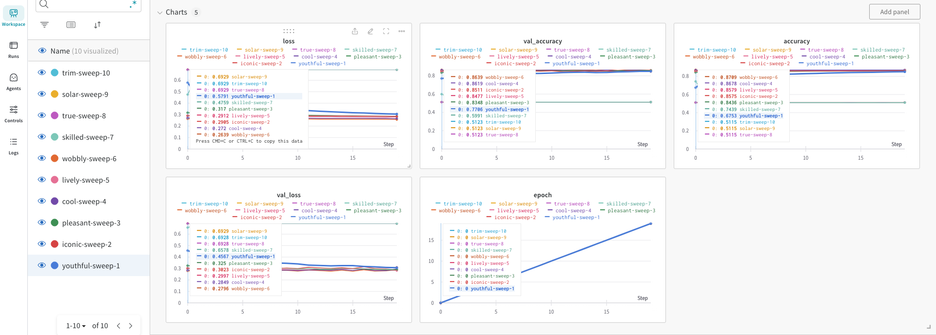
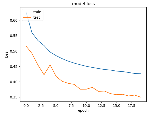
The best model is ‘lively-sweep-5‘ with the lowest validation loss
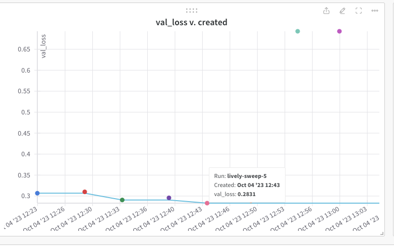
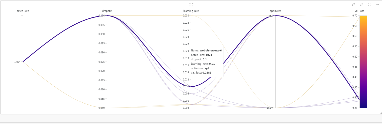
The picture below gives the validation loss for various combinations of the hyper-para meters
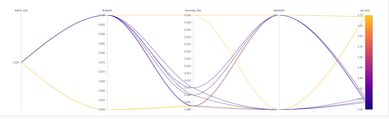
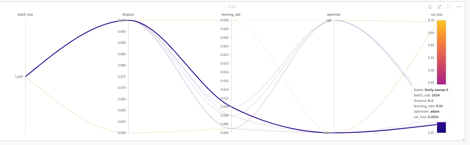
It is very easy to visually pick the best model with loss as shown below. It is lively-sweep-5. we can see the values of the hyper-parameters for this DL model
Details of optimal Deep Learning model
a. Run – lively-sweep-5
b. optimizer – adam
c. learning_rate – 0.01
d. batch_size – 1024
e. dropout – 0.1
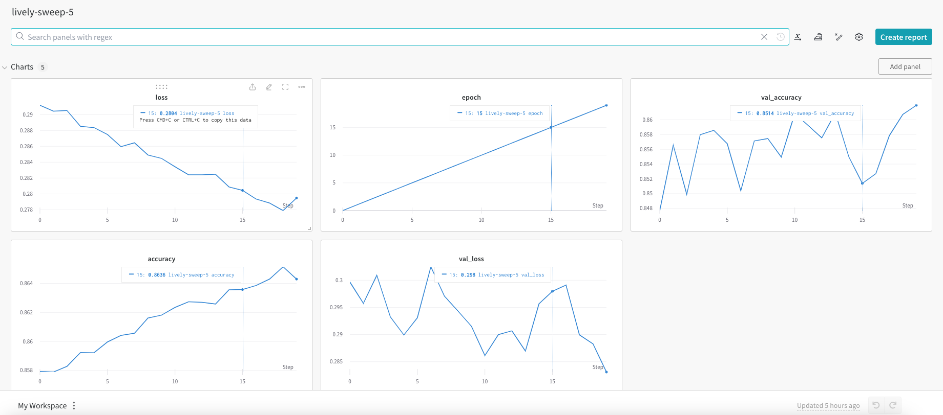
We can see the performance of this model individually by clicking lively-sweep-6 on the left panel
It was good fun to play around with the Weights and Biases in selecting an optimal model
See also
- Deconstructing Convolutional Neural Networks with Tensorflow and Keras
- Deep Learning from first principles in Python, R and Octave – Part 7
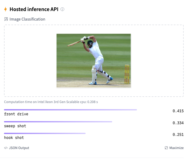
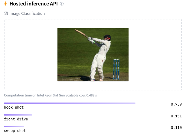
- Identifying cricketing shots using AI
- Introducing cricket package yorkr: Part 2-Trapped leg before wicket!
- Introducing cricpy:A python package to analyze performances of cricketers
To see all posts click Index of posts


 and
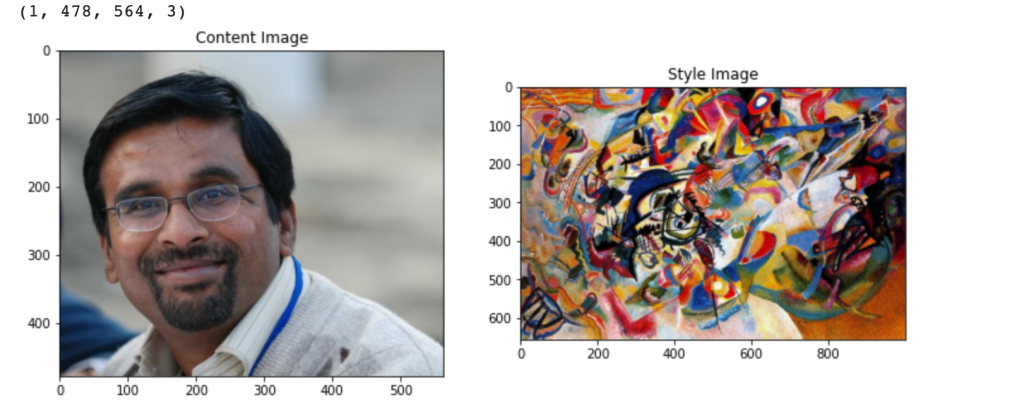
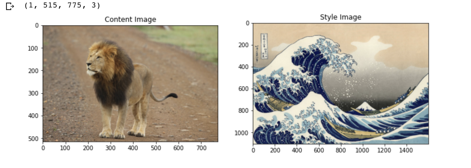
and  represent the activations at layer ‘l’ in a filter i, at position ‘j’. The intuition is that the activations will be same for similar source and generated image. We need to minimise the content loss so that the generated stylized image is as close to the original image as possible. An intermediate layer of VGG19 block5_conv2 is used
 x
x 
 and width
  with
with  channels
 and
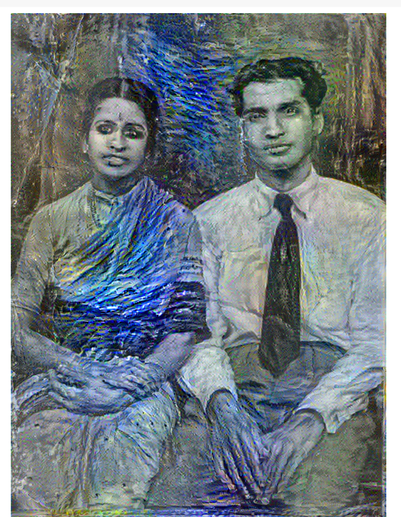
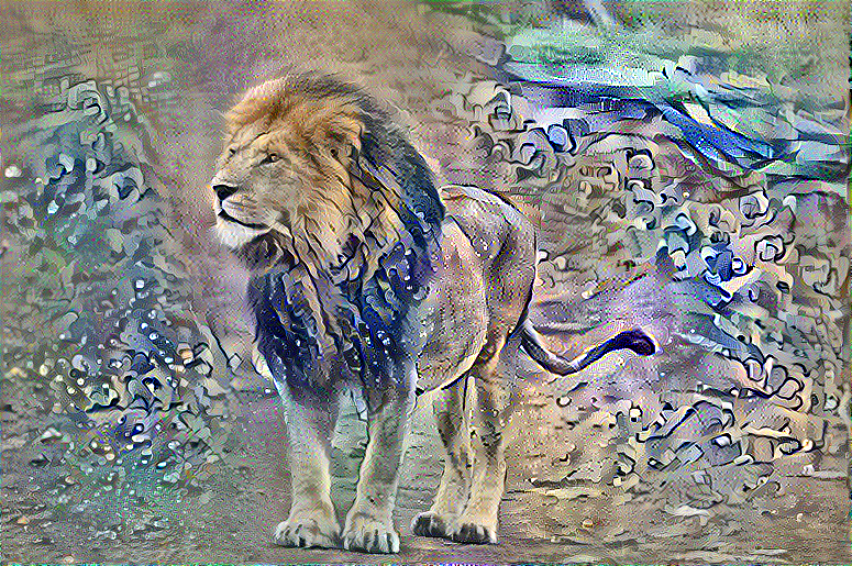
and  are the Gram matrices of the style and generated images respectively. By minimising the distance in the gram matrices of the style and generated image we can ensure that generated image is a stylized version of the original image similar to the style image