Practical Machine Learning with R and Python – Part 5

This is the 5th and probably penultimate part of my series on ‘Practical Machine Learning with R and Python’. The earlier parts of this series included

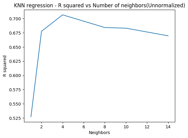
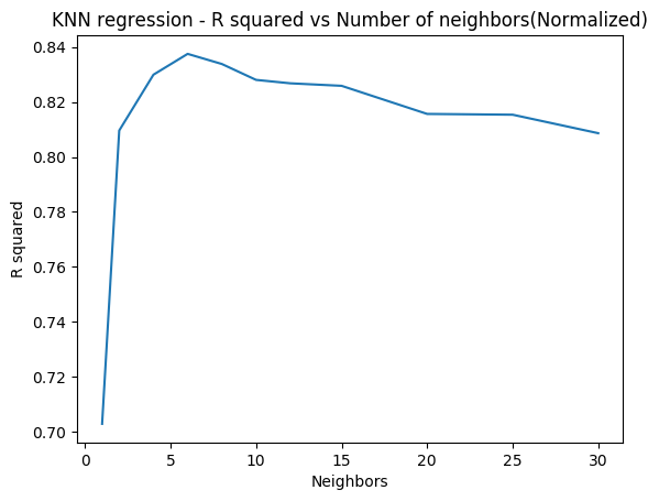
1. Practical Machine Learning with R and Python – Part 1 In this initial post, I touch upon univariate, multivariate, polynomial regression and KNN regression in R and Python
2.Practical Machine Learning with R and Python – Part 2 In this post, I discuss Logistic Regression, KNN classification and cross validation error for both LOOCV and K-Fold in both R and Python
3.Practical Machine Learning with R and Python – Part 3 This post covered ‘feature selection’ in Machine Learning. Specifically I touch best fit, forward fit, backward fit, ridge(L2 regularization) & lasso (L1 regularization). The post includes equivalent code in R and Python.
4.Practical Machine Learning with R and Python – Part 4 In this part I discussed SVMs, Decision Trees, validation, precision recall, and roc curves

This post ‘Practical Machine Learning with R and Python – Part 5’ discusses regression with B-splines, natural splines, smoothing splines, generalized additive models (GAMS), bagging, random forest and boosting

As with my previous posts in this series, this post is largely based on the following 2 MOOC courses

1. Statistical Learning, Prof Trevor Hastie & Prof Robert Tibesherani, Online Stanford
2. Applied Machine Learning in Python Prof Kevyn-Collin Thomson, University Of Michigan, Coursera

You can download this R Markdown file and associated data files from Github at MachineLearning-RandPython-Part5

Note: Please listen to my video presentations Machine Learning in youtube
1. Machine Learning in plain English-Part 1
2. Machine Learning in plain English-Part 2
3. Machine Learning in plain English-Part 3

Check out my compact and minimal book “Practical Machine Learning with R and Python:Third edition- Machine Learning in stereo” available in Amazon in paperback($12.99) and kindle($8.99) versions. My book includes implementations of key ML algorithms and associated measures and metrics. The book is ideal for anybody who is familiar with the concepts and would like a quick reference to the different ML algorithms that can be applied to problems and how to select the best model. Pick your copy today!!

For this part I have used the data sets from UCI Machine Learning repository(Communities and Crime and Auto MPG)

1. Splines

When performing regression (continuous or logistic) between a target variable and a feature (or a set of features), a single polynomial for the entire range of the data set usually does not perform a good fit.Rather we would need to provide we could fit
regression curves for different section of the data set.

There are several techniques which do this for e.g. piecewise-constant functions, piecewise-linear functions, piecewise-quadratic/cubic/4th order polynomial functions etc. One such set of functions are the cubic splines which fit cubic polynomials to successive sections of the dataset. The points where the cubic splines join, are called ‘knots’.

Since each section has a different cubic spline, there could be discontinuities (or breaks) at these knots. To prevent these discontinuities ‘natural splines’ and ‘smoothing splines’ ensure that the seperate cubic functions have 2nd order continuity at these knots with the adjacent splines. 2nd order continuity implies that the value, 1st order derivative and 2nd order derivative at these knots are equal.

A cubic spline with knots $\alpha_{k}$ , k=1,2,3,..K is a piece-wise cubic polynomial with continuous derivative up to order 2 at each knot. We can write $y_{i} = \beta_{0} +\beta_{1}b_{1}(x_{i}) +\beta_{2}b_{2}(x_{i}) + .. + \beta_{K+3}b_{K+3}(x_{i}) + \epsilon_{i}$ .
For each ( $x{i},y{i}$ ), $b_{i}$ are called ‘basis’ functions, where $b_{1}(x_{i})=x_{i}$ , $b_{2}(x_{i})=x_{i}^2$ , $b_{3}(x_{i})=x_{i}^3$ , $b_{k+3}(x_{i})=(x_{i} -\alpha_{k})^3$ where k=1,2,3… K The 1st and 2nd derivatives of cubic splines are continuous at the knots. Hence splines provide a smooth continuous fit to the data by fitting different splines to different sections of the data

1.1a Fit a 4th degree polynomial – R code

In the code below a non-linear function (a 4th order polynomial) is used to fit the data. Usually when we fit a single polynomial to the entire data set the tails of the fit tend to vary a lot particularly if there are fewer points at the ends. Splines help in reducing this variation at the extremities

library(dplyr)
library(ggplot2)
source('RFunctions-1.R')
# Read the data
df=read.csv("auto_mpg.csv",stringsAsFactors = FALSE) # Data from UCI
df1 <- as.data.frame(sapply(df,as.numeric))
#Select specific columns
df2 <- df1 %>% dplyr::select(cylinder,displacement, horsepower,weight, acceleration, year,mpg)
auto <- df2[complete.cases(df2),]
# Fit a 4th degree polynomial
fit=lm(mpg~poly(horsepower,4),data=auto)
#Display a summary of fit
summary(fit)

## 
## Call:
## lm(formula = mpg ~ poly(horsepower, 4), data = auto)
## 
## Residuals:
##      Min       1Q   Median       3Q      Max 
## -14.8820  -2.5802  -0.1682   2.2100  16.1434 
## 
## Coefficients:
##                       Estimate Std. Error t value Pr(>|t|)    
## (Intercept)            23.4459     0.2209 106.161   <2e-16 ***
## poly(horsepower, 4)1 -120.1377     4.3727 -27.475   <2e-16 ***
## poly(horsepower, 4)2   44.0895     4.3727  10.083   <2e-16 ***
## poly(horsepower, 4)3   -3.9488     4.3727  -0.903    0.367    
## poly(horsepower, 4)4   -5.1878     4.3727  -1.186    0.236    
## ---
## Signif. codes:  0 '***' 0.001 '**' 0.01 '*' 0.05 '.' 0.1 ' ' 1
## 
## Residual standard error: 4.373 on 387 degrees of freedom
## Multiple R-squared:  0.6893, Adjusted R-squared:  0.6861 
## F-statistic: 214.7 on 4 and 387 DF,  p-value: < 2.2e-16

#Get the range of horsepower
hp <- range(auto$horsepower)
#Create a sequence to be used for plotting
hpGrid <- seq(hp[1],hp[2],by=10)
#Predict for these values of horsepower. Set Standard error as TRUE
pred=predict(fit,newdata=list(horsepower=hpGrid),se=TRUE)
#Compute bands on either side that is 2xSE
seBands=cbind(pred$fit+2*pred$se.fit,pred$fit-2*pred$se.fit)
#Plot the fit with Standard Error bands
plot(auto$horsepower,auto$mpg,xlim=hp,cex=.5,col="black",xlab="Horsepower",
     ylab="MPG", main="Polynomial of degree 4")
lines(hpGrid,pred$fit,lwd=2,col="blue")
matlines(hpGrid,seBands,lwd=2,col="blue",lty=3)

fig1-1

1.1b Fit a 4th degree polynomial – Python code

import numpy as np
import pandas as pd
import os
import matplotlib.pyplot as plt
from sklearn.model_selection import train_test_split
from sklearn.preprocessing import PolynomialFeatures
from sklearn.linear_model import LinearRegression
#Read the auto data
autoDF =pd.read_csv("auto_mpg.csv",encoding="ISO-8859-1")
# Select columns
autoDF1=autoDF[['mpg','cylinder','displacement','horsepower','weight','acceleration','year']]
# Convert all columns to numeric
autoDF2 = autoDF1.apply(pd.to_numeric, errors='coerce')

#Drop NAs
autoDF3=autoDF2.dropna()
autoDF3.shape
X=autoDF3[['horsepower']]
y=autoDF3['mpg']
#Create a polynomial of degree 4
poly = PolynomialFeatures(degree=4)
X_poly = poly.fit_transform(X)

# Fit a polynomial regression line
linreg = LinearRegression().fit(X_poly, y)
# Create a range of values
hpGrid = np.arange(np.min(X),np.max(X),10)
hp=hpGrid.reshape(-1,1)
# Transform to 4th degree
poly = PolynomialFeatures(degree=4)
hp_poly = poly.fit_transform(hp)

#Create a scatter plot
plt.scatter(X,y)
# Fit the prediction
ypred=linreg.predict(hp_poly)
plt.title("Poylnomial of degree 4")
fig2=plt.xlabel("Horsepower")
fig2=plt.ylabel("MPG")
# Draw the regression curve
plt.plot(hp,ypred,c="red")
plt.savefig('fig1.png', bbox_inches='tight')

1.1c Fit a B-Spline – R Code

In the code below a B- Spline is fit to data. The B-spline requires the manual selection of knots

#Splines
library(splines)
# Fit a B-spline to the data. Select knots at 60,75,100,150
fit=lm(mpg~bs(horsepower,df=6,knots=c(60,75,100,150)),data=auto)
# Use the fitted regresion to predict
pred=predict(fit,newdata=list(horsepower=hpGrid),se=T)
# Create a scatter plot
plot(auto$horsepower,auto$mpg,xlim=hp,cex=.5,col="black",xlab="Horsepower",
     ylab="MPG", main="B-Spline with 4 knots")
#Draw lines with 2 Standard Errors on either side
lines(hpGrid,pred$fit,lwd=2)
lines(hpGrid,pred$fit+2*pred$se,lty="dashed")
lines(hpGrid,pred$fit-2*pred$se,lty="dashed")
abline(v=c(60,75,100,150),lty=2,col="darkgreen")

fig2-1

1.1d Fit a Natural Spline – R Code

Here a ‘Natural Spline’ is used to fit .The Natural Spline extrapolates beyond the boundary knots and the ends of the function are much more constrained than a regular spline or a global polynomoial where the ends can wag a lot more. Natural splines do not require the explicit selection of knots

# There is no need to select the knots here. There is a smoothing parameter which
# can be specified by the degrees of freedom 'df' parameter. The natural spline

fit2=lm(mpg~ns(horsepower,df=4),data=auto)
pred=predict(fit2,newdata=list(horsepower=hpGrid),se=T)
plot(auto$horsepower,auto$mpg,xlim=hp,cex=.5,col="black",xlab="Horsepower",
     ylab="MPG", main="Natural Splines")
lines(hpGrid,pred$fit,lwd=2)
lines(hpGrid,pred$fit+2*pred$se,lty="dashed")
lines(hpGrid,pred$fit-2*pred$se,lty="dashed")

fig3-1

1.1.e Fit a Smoothing Spline – R code

Here a smoothing spline is used. Smoothing splines also do not require the explicit setting of knots. We can change the ‘degrees of freedom(df)’ paramater to get the best fit

# Smoothing spline has a smoothing parameter, the degrees of freedom
# This is too wiggly
plot(auto$horsepower,auto$mpg,xlim=hp,cex=.5,col="black",xlab="Horsepower",
     ylab="MPG", main="Smoothing Splines")

# Here df is set to 16. This has a lot of variance
fit=smooth.spline(auto$horsepower,auto$mpg,df=16)
lines(fit,col="red",lwd=2)

# We can use Cross Validation to allow the spline to pick the value of this smpopothing paramter. We do not need to set the degrees of freedom 'df'
fit=smooth.spline(auto$horsepower,auto$mpg,cv=TRUE)
lines(fit,col="blue",lwd=2)

fig4-1

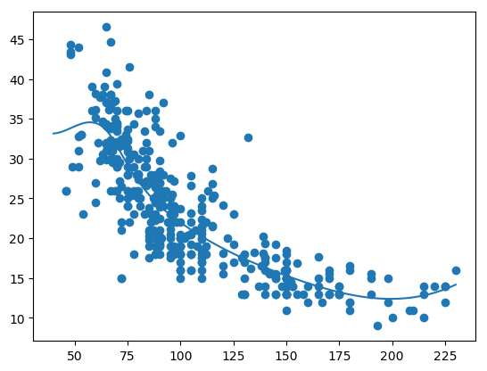
1.1e Splines – Python

There isn’t as much treatment of splines in Python and SKLearn. I did find the LSQUnivariate, UnivariateSpline spline. The LSQUnivariate spline requires the explcit setting of knots

import numpy as np
import pandas as pd
import os
import matplotlib.pyplot as plt
from scipy.interpolate import LSQUnivariateSpline
autoDF =pd.read_csv("auto_mpg.csv",encoding="ISO-8859-1")
autoDF.shape
autoDF.columns
autoDF1=autoDF[['mpg','cylinder','displacement','horsepower','weight','acceleration','year']]
autoDF2 = autoDF1.apply(pd.to_numeric, errors='coerce')
auto=autoDF2.dropna()
auto=auto[['horsepower','mpg']].sort_values('horsepower')

# Set the knots manually
knots=[65,75,100,150]
# Create an array for X & y
X=np.array(auto['horsepower'])
y=np.array(auto['mpg'])
# Fit a LSQunivariate spline
s = LSQUnivariateSpline(X,y,knots)

#Plot the spline
xs = np.linspace(40,230,1000)
ys = s(xs)
plt.scatter(X, y)
plt.plot(xs, ys)
plt.savefig('fig2.png', bbox_inches='tight')

1.2 Generalized Additiive models (GAMs)

Generalized Additive Models (GAMs) is a really powerful ML tool.

y_{i} = \beta_{0} + f_{1}(x_{i1}) + f_{2}(x_{i2}) + .. +f_{p}(x_{ip}) + \epsilon_{i}

In GAMs we use a different functions for each of the variables. GAMs give a much better fit since we can choose any function for the different sections

1.2a Generalized Additive Models (GAMs) – R Code

The plot below show the smooth spline that is fit for each of the features horsepower, cylinder, displacement, year and acceleration. We can use any function for example loess, 4rd order polynomial etc.

library(gam)
# Fit a smoothing spline for horsepower, cyliner, displacement and acceleration
gam=gam(mpg~s(horsepower,4)+s(cylinder,5)+s(displacement,4)+s(year,4)+s(acceleration,5),data=auto)
# Display the summary of the fit. This give the significance of each of the paramwetr
# Also an ANOVA is given for each combination of the features
summary(gam)

## 
## Call: gam(formula = mpg ~ s(horsepower, 4) + s(cylinder, 5) + s(displacement, 
##     4) + s(year, 4) + s(acceleration, 5), data = auto)
## Deviance Residuals:
##     Min      1Q  Median      3Q     Max 
## -8.3190 -1.4436 -0.0261  1.2279 12.0873 
## 
## (Dispersion Parameter for gaussian family taken to be 6.9943)
## 
##     Null Deviance: 23818.99 on 391 degrees of freedom
## Residual Deviance: 2587.881 on 370 degrees of freedom
## AIC: 1898.282 
## 
## Number of Local Scoring Iterations: 3 
## 
## Anova for Parametric Effects
##                     Df  Sum Sq Mean Sq  F value    Pr(>F)    
## s(horsepower, 4)     1 15632.8 15632.8 2235.085 < 2.2e-16 ***
## s(cylinder, 5)       1   508.2   508.2   72.666 3.958e-16 ***
## s(displacement, 4)   1   374.3   374.3   53.514 1.606e-12 ***
## s(year, 4)           1  2263.2  2263.2  323.583 < 2.2e-16 ***
## s(acceleration, 5)   1   372.4   372.4   53.246 1.809e-12 ***
## Residuals          370  2587.9     7.0                       
## ---
## Signif. codes:  0 '***' 0.001 '**' 0.01 '*' 0.05 '.' 0.1 ' ' 1
## 
## Anova for Nonparametric Effects
##                    Npar Df Npar F     Pr(F)    
## (Intercept)                                    
## s(horsepower, 4)         3 13.825 1.453e-08 ***
## s(cylinder, 5)           3 17.668 9.712e-11 ***
## s(displacement, 4)       3 44.573 < 2.2e-16 ***
## s(year, 4)               3 23.364 7.183e-14 ***
## s(acceleration, 5)       4  3.848  0.004453 ** 
## ---
## Signif. codes:  0 '***' 0.001 '**' 0.01 '*' 0.05 '.' 0.1 ' ' 1

par(mfrow=c(2,3))
plot(gam,se=TRUE)

fig5-1

1.2b Generalized Additive Models (GAMs) – Python Code

I did not find the equivalent of GAMs in SKlearn in Python. There was an early prototype (2012) in Github. Looks like it is still work in progress or has probably been abandoned.

1.3 Tree based Machine Learning Models

Tree based Machine Learning are all based on the ‘bootstrapping’ technique. In bootstrapping given a sample of size N, we create datasets of size N by sampling this original dataset with replacement. Machine Learning models are built on the different bootstrapped samples and then averaged.

Decision Trees as seen above have the tendency to overfit. There are several techniques that help to avoid this namely a) Bagging b) Random Forests c) Boosting

Bagging, Random Forest and Gradient Boosting

Bagging: Bagging, or Bootstrap Aggregation decreases the variance of predictions, by creating separate Decisiion Tree based ML models on the different samples and then averaging these ML models

Random Forests: Bagging is a greedy algorithm and tries to produce splits based on all variables which try to minimize the error. However the different ML models have a high correlation. Random Forests remove this shortcoming, by using a variable and random set of features to split on. Hence the features chosen and the resulting trees are uncorrelated. When these ML models are averaged the performance is much better.

Boosting: Gradient Boosted Decision Trees also use an ensemble of trees but they don’t build Machine Learning models with random set of features at each step. Rather small and simple trees are built. Successive trees try to minimize the error from the earlier trees.

Out of Bag (OOB) Error: In Random Forest and Gradient Boosting for each bootstrap sample taken from the dataset, there will be samples left out. These are known as Out of Bag samples.Classification accuracy carried out on these OOB samples is known as OOB error

1.31a Decision Trees – R Code

The code below creates a Decision tree with the cancer training data. The summary of the fit is output. Based on the ML model, the predict function is used on test data and a confusion matrix is output.

# Read the cancer data
library(tree)
library(caret)
library(e1071)
cancer <- read.csv("cancer.csv",stringsAsFactors = FALSE)
cancer <- cancer[,2:32]
cancer$target <- as.factor(cancer$target)
train_idx <- trainTestSplit(cancer,trainPercent=75,seed=5)
train <- cancer[train_idx, ]
test <- cancer[-train_idx, ]

# Create Decision Tree
cancerStatus=tree(target~.,train)
summary(cancerStatus)

## 
## Classification tree:
## tree(formula = target ~ ., data = train)
## Variables actually used in tree construction:
## [1] "worst.perimeter"      "worst.concave.points" "area.error"          
## [4] "worst.texture"        "mean.texture"         "mean.concave.points" 
## Number of terminal nodes:  9 
## Residual mean deviance:  0.1218 = 50.8 / 417 
## Misclassification error rate: 0.02347 = 10 / 426

pred <- predict(cancerStatus,newdata=test,type="class")
confusionMatrix(pred,test$target)

## Confusion Matrix and Statistics
## 
##           Reference
## Prediction  0  1
##          0 49  7
##          1  8 78
##                                           
##                Accuracy : 0.8944          
##                  95% CI : (0.8318, 0.9397)
##     No Information Rate : 0.5986          
##     P-Value [Acc > NIR] : 4.641e-15       
##                                           
##                   Kappa : 0.7795          
##  Mcnemar's Test P-Value : 1               
##                                           
##             Sensitivity : 0.8596          
##             Specificity : 0.9176          
##          Pos Pred Value : 0.8750          
##          Neg Pred Value : 0.9070          
##              Prevalence : 0.4014          
##          Detection Rate : 0.3451          
##    Detection Prevalence : 0.3944          
##       Balanced Accuracy : 0.8886          
##                                           
##        'Positive' Class : 0               
##

# Plot decision tree with labels
plot(cancerStatus)
text(cancerStatus,pretty=0)

fig6-1

1.31b Decision Trees – Cross Validation – R Code

We can also perform a Cross Validation on the data to identify the Decision Tree which will give the minimum deviance.

library(tree)
cancer <- read.csv("cancer.csv",stringsAsFactors = FALSE)
cancer <- cancer[,2:32]
cancer$target <- as.factor(cancer$target)
train_idx <- trainTestSplit(cancer,trainPercent=75,seed=5)
train <- cancer[train_idx, ]
test <- cancer[-train_idx, ]

# Create Decision Tree
cancerStatus=tree(target~.,train)

# Execute 10 fold cross validation
cvCancer=cv.tree(cancerStatus)
plot(cvCancer)

fig7-1

# Plot the 
plot(cvCancer$size,cvCancer$dev,type='b')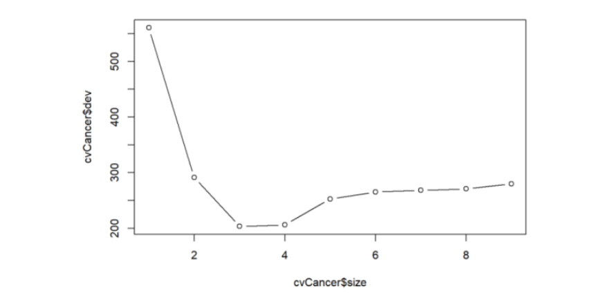

fig1

prunedCancer=prune.tree(cancerStatus,best=4)
plot(prunedCancer)
text(prunedCancer,pretty=0)

fig2

pred <- predict(prunedCancer,newdata=test,type="class")
confusionMatrix(pred,test$target)

## Confusion Matrix and Statistics
## 
##           Reference
## Prediction  0  1
##          0 50  7
##          1  7 78
##                                          
##                Accuracy : 0.9014         
##                  95% CI : (0.8401, 0.945)
##     No Information Rate : 0.5986         
##     P-Value [Acc > NIR] : 7.988e-16      
##                                          
##                   Kappa : 0.7948         
##  Mcnemar's Test P-Value : 1              
##                                          
##             Sensitivity : 0.8772         
##             Specificity : 0.9176         
##          Pos Pred Value : 0.8772         
##          Neg Pred Value : 0.9176         
##              Prevalence : 0.4014         
##          Detection Rate : 0.3521         
##    Detection Prevalence : 0.4014         
##       Balanced Accuracy : 0.8974         
##                                          
##        'Positive' Class : 0              
##

1.31c Decision Trees – Python Code

Below is the Python code for creating Decision Trees. The accuracy, precision, recall and F1 score is computed on the test data set.

import numpy as np
import pandas as pd
import os
import matplotlib.pyplot as plt
from sklearn.metrics import confusion_matrix
from sklearn import tree
from sklearn.datasets import load_breast_cancer
from sklearn.model_selection import train_test_split
from sklearn.tree import DecisionTreeClassifier
from sklearn.datasets import make_classification, make_blobs
from sklearn.metrics import accuracy_score, precision_score, recall_score, f1_score
import graphviz 

cancer = load_breast_cancer()
(X_cancer, y_cancer) = load_breast_cancer(return_X_y = True)

X_train, X_test, y_train, y_test = train_test_split(X_cancer, y_cancer,
                                                   random_state = 0)
clf = DecisionTreeClassifier().fit(X_train, y_train)

print('Accuracy of Decision Tree classifier on training set: {:.2f}'
     .format(clf.score(X_train, y_train)))
print('Accuracy of Decision Tree classifier on test set: {:.2f}'
     .format(clf.score(X_test, y_test)))

y_predicted=clf.predict(X_test)
confusion = confusion_matrix(y_test, y_predicted)
print('Accuracy: {:.2f}'.format(accuracy_score(y_test, y_predicted)))
print('Precision: {:.2f}'.format(precision_score(y_test, y_predicted)))
print('Recall: {:.2f}'.format(recall_score(y_test, y_predicted)))
print('F1: {:.2f}'.format(f1_score(y_test, y_predicted)))

# Plot the Decision Tree
clf = DecisionTreeClassifier(max_depth=2).fit(X_train, y_train)
dot_data = tree.export_graphviz(clf, out_file=None, 
                         feature_names=cancer.feature_names,  
                         class_names=cancer.target_names,  
                         filled=True, rounded=True,  
                         special_characters=True)  
graph = graphviz.Source(dot_data)  
graph

## Accuracy of Decision Tree classifier on training set: 1.00
## Accuracy of Decision Tree classifier on test set: 0.87
## Accuracy: 0.87
## Precision: 0.97
## Recall: 0.82
## F1: 0.89

1.31d Decision Trees – Cross Validation – Python Code

In the code below 5-fold cross validation is performed for different depths of the tree and the accuracy is computed. The accuracy on the test set seems to plateau when the depth is 8. But it is seen to increase again from 10 to 12. More analysis needs to be done here


import numpy as np
import pandas as pd
import os
import matplotlib.pyplot as plt
from sklearn.datasets import load_breast_cancer
from sklearn.tree import DecisionTreeClassifier
(X_cancer, y_cancer) = load_breast_cancer(return_X_y = True)
from sklearn.cross_validation import train_test_split, KFold
def computeCVAccuracy(X,y,folds):
    accuracy=[]
    foldAcc=[]
    depth=[1,2,3,4,5,6,7,8,9,10,11,12]
    nK=len(X)/float(folds)
    xval_err=0
    for i in depth: 
        kf = KFold(len(X),n_folds=folds)
        for train_index, test_index in kf:
            X_train, X_test = X.iloc[train_index], X.iloc[test_index]
            y_train, y_test = y.iloc[train_index], y.iloc[test_index]  
            clf = DecisionTreeClassifier(max_depth = i).fit(X_train, y_train)
            score=clf.score(X_test, y_test)
            accuracy.append(score)     
            
        foldAcc.append(np.mean(accuracy))  
        
    return(foldAcc)
    
    
cvAccuracy=computeCVAccuracy(pd.DataFrame(X_cancer),pd.DataFrame(y_cancer),folds=10)

df1=pd.DataFrame(cvAccuracy)
df1.columns=['cvAccuracy']
df=df1.reindex([1,2,3,4,5,6,7,8,9,10,11,12])
df.plot()
plt.title("Decision Tree - 10-fold Cross Validation Accuracy vs Depth of tree")
plt.xlabel("Depth of tree")
plt.ylabel("Accuracy")
plt.savefig('fig3.png', bbox_inches='tight')

1.4a Random Forest – R code

A Random Forest is fit using the Boston data. The summary shows that 4 variables were randomly chosen at each split and the resulting ML model explains 88.72% of the test data. Also the variable importance is plotted. It can be seen that ‘rooms’ and ‘status’ are the most influential features in the model

library(randomForest)
df=read.csv("Boston.csv",stringsAsFactors = FALSE) # Data from MASS - SL

# Select specific columns
Boston <- df %>% dplyr::select("crimeRate","zone","indus","charles","nox","rooms","age",                          "distances","highways","tax","teacherRatio","color",
                               "status","medianValue")

# Fit a Random Forest on the Boston training data
rfBoston=randomForest(medianValue~.,data=Boston)
# Display the summatu of the fit. It can be seen that the MSE is 10.88 
# and the percentage variance explained is 86.14%. About 4 variables were tried at each # #split for a maximum tree of 500.
# The MSE and percent variance is on Out of Bag trees
rfBoston

## 
## Call:
##  randomForest(formula = medianValue ~ ., data = Boston) 
##                Type of random forest: regression
##                      Number of trees: 500
## No. of variables tried at each split: 4
## 
##           Mean of squared residuals: 9.521672
##                     % Var explained: 88.72

#List and plot the variable importances
importance(rfBoston)

##              IncNodePurity
## crimeRate        2602.1550
## zone              258.8057
## indus            2599.6635
## charles           240.2879
## nox              2748.8485
## rooms           12011.6178
## age              1083.3242
## distances        2432.8962
## highways          393.5599
## tax              1348.6987
## teacherRatio     2841.5151
## color             731.4387
## status          12735.4046

varImpPlot(rfBoston)

fig8-1

1.4b Random Forest-OOB and Cross Validation Error – R code

The figure below shows the OOB error and the Cross Validation error vs the ‘mtry’. Here mtry indicates the number of random features that are chosen at each split. The lowest test error occurs when mtry = 8

library(randomForest)
df=read.csv("Boston.csv",stringsAsFactors = FALSE) # Data from MASS - SL

# Select specific columns
Boston <- df %>% dplyr::select("crimeRate","zone","indus","charles","nox","rooms","age",                          "distances","highways","tax","teacherRatio","color",
                               "status","medianValue")
# Split as training and tst sets
train_idx <- trainTestSplit(Boston,trainPercent=75,seed=5)
train <- Boston[train_idx, ]
test <- Boston[-train_idx, ]

#Initialize OOD and testError
oobError <- NULL
testError <- NULL
# In the code below the number of variables to consider at each split is increased
# from 1 - 13(max features) and the OOB error and the MSE is computed
for(i in 1:13){
    fitRF=randomForest(medianValue~.,data=train,mtry=i,ntree=400)
    oobError[i] <-fitRF$mse[400]
    pred <- predict(fitRF,newdata=test)
    testError[i] <- mean((pred-test$medianValue)^2)
}

# We can see the OOB and Test Error. It can be seen that the Random Forest performs
# best with the lowers MSE at mtry=6
matplot(1:13,cbind(testError,oobError),pch=19,col=c("red","blue"),
        type="b",xlab="mtry(no of varaibles at each split)", ylab="Mean Squared Error",
        main="Random Forest - OOB and Test Error")
legend("topright",legend=c("OOB","Test"),pch=19,col=c("red","blue"))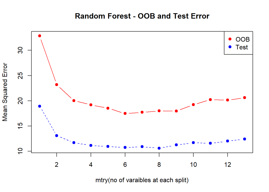

fig9-1

1.4c Random Forest – Python code

The python code for Random Forest Regression is shown below. The training and test score is computed. The variable importance shows that ‘rooms’ and ‘status’ are the most influential of the variables

import numpy as np
import pandas as pd
import os
import matplotlib.pyplot as plt
from sklearn.model_selection import train_test_split
from sklearn.ensemble import RandomForestRegressor
df = pd.read_csv("Boston.csv",encoding = "ISO-8859-1")

X=df[['crimeRate','zone', 'indus','charles','nox','rooms', 'age','distances','highways','tax',
       'teacherRatio','color','status']]
y=df['medianValue']

X_train, X_test, y_train, y_test = train_test_split(X, y, random_state = 0)

regr = RandomForestRegressor(max_depth=4, random_state=0)
regr.fit(X_train, y_train)

print('R-squared score (training): {:.3f}'
     .format(regr.score(X_train, y_train)))
print('R-squared score (test): {:.3f}'
     .format(regr.score(X_test, y_test)))

feature_names=['crimeRate','zone', 'indus','charles','nox','rooms', 'age','distances','highways','tax',
       'teacherRatio','color','status']
print(regr.feature_importances_)
plt.figure(figsize=(10,6),dpi=80)
c_features=X_train.shape[1]
plt.barh(np.arange(c_features),regr.feature_importances_)
plt.xlabel("Feature importance")
plt.ylabel("Feature name")

plt.yticks(np.arange(c_features), feature_names)
plt.tight_layout()

plt.savefig('fig4.png', bbox_inches='tight')

## R-squared score (training): 0.917
## R-squared score (test): 0.734
## [ 0.03437382  0.          0.00580335  0.          0.00731004  0.36461548
##   0.00638577  0.03432173  0.0041244   0.01732328  0.01074148  0.0012638
##   0.51373683]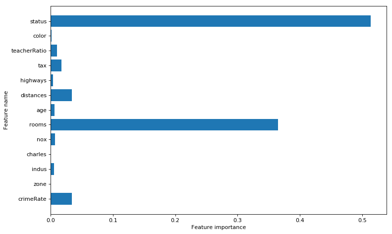

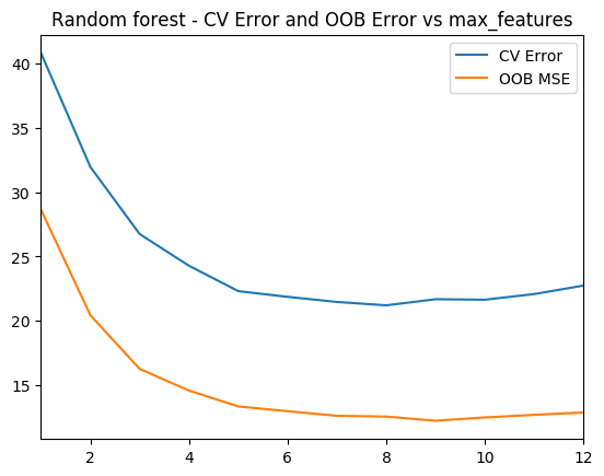
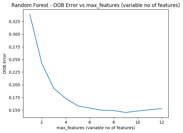
1.4d Random Forest – Cross Validation and OOB Error – Python code

As with R the ‘max_features’ determines the random number of features the random forest will use at each split. The plot shows that when max_features=8 the MSE is lowest

import numpy as np
import pandas as pd
import os
import matplotlib.pyplot as plt
from sklearn.model_selection import train_test_split
from sklearn.ensemble import RandomForestRegressor
from sklearn.model_selection import cross_val_score
df = pd.read_csv("Boston.csv",encoding = "ISO-8859-1")

X=df[['crimeRate','zone', 'indus','charles','nox','rooms', 'age','distances','highways','tax',
       'teacherRatio','color','status']]
y=df['medianValue']

cvError=[]
oobError=[]
oobMSE=[]
for i in range(1,13):
    regr = RandomForestRegressor(max_depth=4, n_estimators=400,max_features=i,oob_score=True,random_state=0)
    mse= np.mean(cross_val_score(regr, X, y, cv=5,scoring = 'neg_mean_squared_error'))
    # Since this is neg_mean_squared_error I have inverted the sign to get MSE
    cvError.append(-mse)
    # Fit on all data to compute OOB error
    regr.fit(X, y)
    # Record the OOB error for each `max_features=i` setting
    oob = 1 - regr.oob_score_
    oobError.append(oob)
    # Get the Out of Bag prediction
    oobPred=regr.oob_prediction_ 
    # Compute the Mean Squared Error between OOB Prediction and target
    mseOOB=np.mean(np.square(oobPred-y))
    oobMSE.append(mseOOB)

# Plot the CV Error and OOB Error
# Set max_features
maxFeatures=np.arange(1,13) 
cvError=pd.DataFrame(cvError,index=maxFeatures)
oobMSE=pd.DataFrame(oobMSE,index=maxFeatures)
#Plot
fig8=df.plot()
fig8=plt.title('Random forest - CV Error and OOB Error vs max_features')
fig8.figure.savefig('fig8.png', bbox_inches='tight')

#Plot the OOB Error vs max_features
plt.plot(range(1,13),oobError)
fig2=plt.title("Random Forest - OOB Error vs max_features (variable no of features)")
fig2=plt.xlabel("max_features (variable no of features)")
fig2=plt.ylabel("OOB Error")
fig2.figure.savefig('fig7.png', bbox_inches='tight')

1.5a Boosting – R code

Here a Gradient Boosted ML Model is built with a n.trees=5000, with a learning rate of 0.01 and depth of 4. The feature importance plot also shows that rooms and status are the 2 most important features. The MSE vs the number of trees plateaus around 2000 trees

library(gbm)
# Perform gradient boosting on the Boston data set. The distribution is gaussian since we
# doing MSE. The interaction depth specifies the number of splits
boostBoston=gbm(medianValue~.,data=train,distribution="gaussian",n.trees=5000,
                shrinkage=0.01,interaction.depth=4)
#The summary gives the variable importance. The 2 most significant variables are
# number of rooms and lower status
summary(boostBoston)

##                       var    rel.inf
## rooms               rooms 42.2267200
## status             status 27.3024671
## distances       distances  7.9447972
## crimeRate       crimeRate  5.0238827
## nox                   nox  4.0616548
## teacherRatio teacherRatio  3.1991999
## age                   age  2.7909772
## color               color  2.3436295
## tax                   tax  2.1386213
## charles           charles  1.3799109
## highways         highways  0.7644026
## indus               indus  0.7236082
## zone                 zone  0.1001287

# The plots below show how each variable relates to the median value of the home. As
# the number of roomd increase the median value increases and with increase in lower status
# the median value decreases
par(mfrow=c(1,2))
#Plot the relation between the top 2 features and the target
plot(boostBoston,i="rooms")
plot(boostBoston,i="status")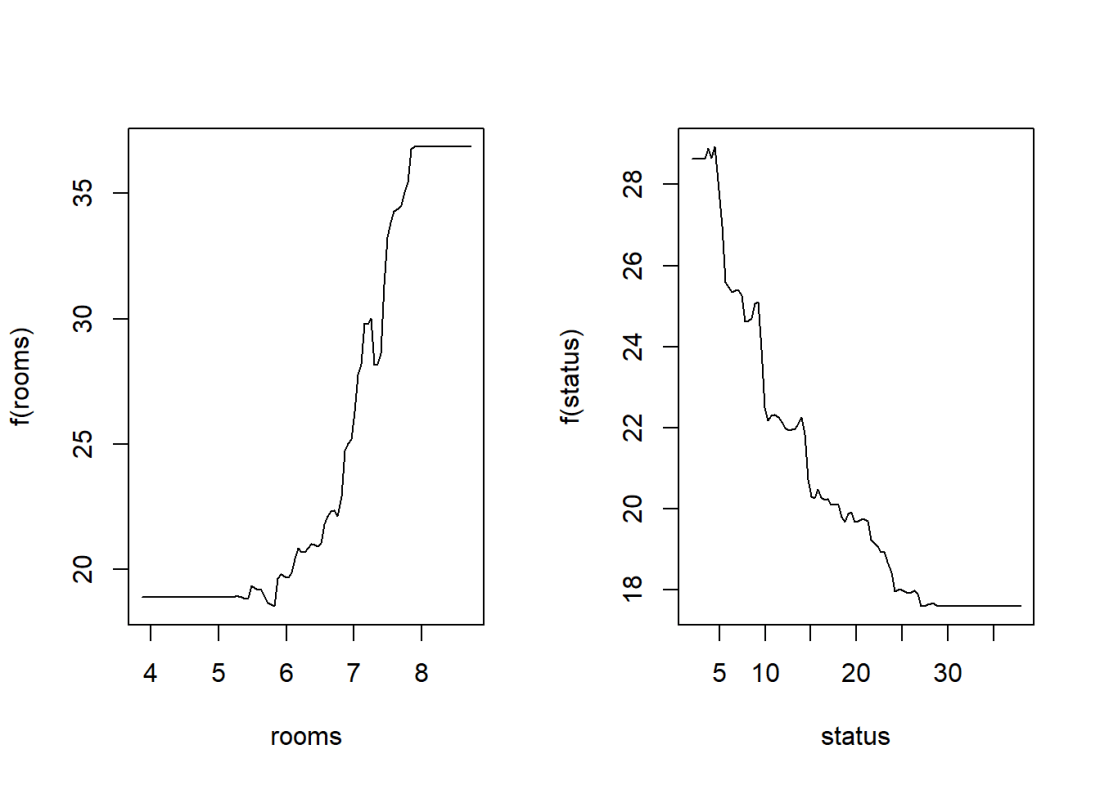

fig10-2

# Create a sequence of trees between 100-5000 incremented by 50
nTrees=seq(100,5000,by=50)
# Predict the values for the test data
pred <- predict(boostBoston,newdata=test,n.trees=nTrees)
# Compute the mean for each of the MSE for each of the number of trees 
boostError <- apply((pred-test$medianValue)^2,2,mean)
#Plot the MSE vs the number of trees
plot(nTrees,boostError,pch=19,col="blue",ylab="Mean Squared Error",
     main="Boosting Test Error")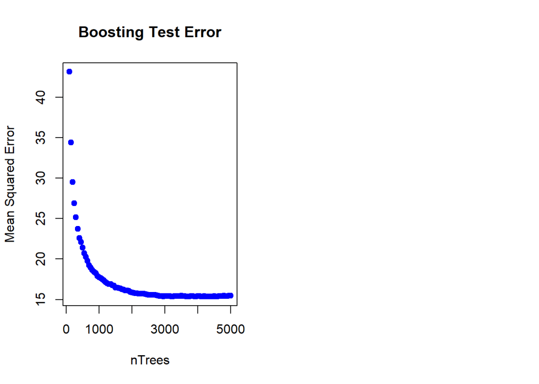

fig10-3

1.5b Cross Validation Boosting – R code

Included below is a cross validation error vs the learning rate. The lowest error is when learning rate = 0.09

cvError <- NULL
s <- c(.001,0.01,0.03,0.05,0.07,0.09,0.1)
for(i in seq_along(s)){
    cvBoost=gbm(medianValue~.,data=train,distribution="gaussian",n.trees=5000,
                shrinkage=s[i],interaction.depth=4,cv.folds=5)
    cvError[i] <- mean(cvBoost$cv.error)
}

# Create a data frame for plotting
a <- rbind(s,cvError)
b <- as.data.frame(t(a))
# It can be seen that a shrinkage parameter of 0,05 gives the lowes CV Error
ggplot(b,aes(s,cvError)) + geom_point() + geom_line(color="blue") + 
    xlab("Shrinkage") + ylab("Cross Validation Error") +
    ggtitle("Gradient boosted trees - Cross Validation error vs Shrinkage")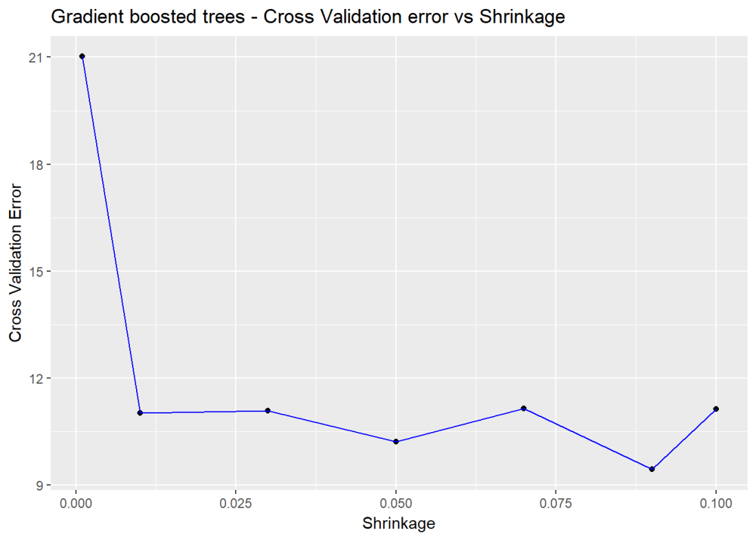

fig11-1

1.5c Boosting – Python code

A gradient boost ML model in Python is created below. The Rsquared score is computed on the training and test data.

import numpy as np
import pandas as pd
import os
import matplotlib.pyplot as plt
from sklearn.model_selection import train_test_split
from sklearn.ensemble import GradientBoostingRegressor
df = pd.read_csv("Boston.csv",encoding = "ISO-8859-1")

X=df[['crimeRate','zone', 'indus','charles','nox','rooms', 'age','distances','highways','tax',
       'teacherRatio','color','status']]
y=df['medianValue']

X_train, X_test, y_train, y_test = train_test_split(X, y, random_state = 0)

regr = GradientBoostingRegressor()
regr.fit(X_train, y_train)

print('R-squared score (training): {:.3f}'
     .format(regr.score(X_train, y_train)))
print('R-squared score (test): {:.3f}'
     .format(regr.score(X_test, y_test)))

## R-squared score (training): 0.983
## R-squared score (test): 0.821

1.5c Cross Validation Boosting – Python code

the cross validation error is computed as the learning rate is varied. The minimum CV eror occurs when lr = 0.04

import numpy as np
import pandas as pd
import os
import matplotlib.pyplot as plt
from sklearn.model_selection import train_test_split
from sklearn.ensemble import RandomForestRegressor
from sklearn.ensemble import GradientBoostingRegressor
from sklearn.model_selection import cross_val_score
df = pd.read_csv("Boston.csv",encoding = "ISO-8859-1")

X=df[['crimeRate','zone', 'indus','charles','nox','rooms', 'age','distances','highways','tax',
       'teacherRatio','color','status']]
y=df['medianValue']

cvError=[]
learning_rate =[.001,0.01,0.03,0.05,0.07,0.09,0.1]
for lr in learning_rate:
    regr = GradientBoostingRegressor(max_depth=4, n_estimators=400,learning_rate  =lr,random_state=0)
    mse= np.mean(cross_val_score(regr, X, y, cv=10,scoring = 'neg_mean_squared_error'))
    # Since this is neg_mean_squared_error I have inverted the sign to get MSE
    cvError.append(-mse)
learning_rate =[.001,0.01,0.03,0.05,0.07,0.09,0.1]
plt.plot(learning_rate,cvError)
plt.title("Gradient Boosting - 5-fold CV- Mean Squared Error vs max_features (variable no of features)")
plt.xlabel("max_features (variable no of features)")
plt.ylabel("Mean Squared Error")
plt.savefig('fig6.png', bbox_inches='tight')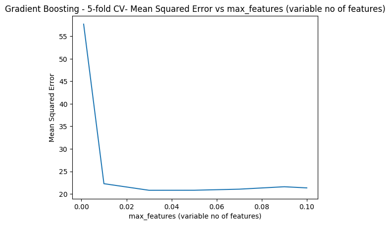

fig6

Conclusion This post covered Splines and Tree based ML models like Bagging, Random Forest and Boosting. Stay tuned for further updates.

Practical Machine Learning with R and Python – Part 4

This is the 4th installment of my ‘Practical Machine Learning with R and Python’ series. In this part I discuss classification with Support Vector Machines (SVMs), using both a Linear and a Radial basis kernel, and Decision Trees. Further, a closer look is taken at some of the metrics associated with binary classification, namely accuracy vs precision and recall. I also touch upon Validation curves, Precision-Recall, ROC curves and AUC with equivalent code in R and Python

This post is a continuation of my 3 earlier posts on Practical Machine Learning in R and Python
1. Practical Machine Learning with R and Python – Part 1
2. Practical Machine Learning with R and Python – Part 2
3. Practical Machine Learning with R and Python – Part 3

The RMarkdown file with the code and the associated data files can be downloaded from Github at MachineLearning-RandPython-Part4

Support Vector Machines (SVM) are another useful Machine Learning model that can be used for both regression and classification problems. SVMs used in classification, compute the hyperplane, that separates the 2 classes with the maximum margin. To do this the features may be transformed into a larger multi-dimensional feature space. SVMs can be used with different kernels namely linear, polynomial or radial basis to determine the best fitting model for a given classification problem.

In the 2nd part of this series Practical Machine Learning with R and Python – Part 2, I had mentioned the various metrics that are used in classification ML problems namely Accuracy, Precision, Recall and F1 score. Accuracy gives the fraction of data that were correctly classified as belonging to the +ve or -ve class. However ‘accuracy’ in itself is not a good enough measure because it does not take into account the fraction of the data that were incorrectly classified. This issue becomes even more critical in different domains. For e.g a surgeon who would like to detect cancer, would like to err on the side of caution, and classify even a possibly non-cancerous patient as possibly having cancer, rather than mis-classifying a malignancy as benign. Here we would like to increase recall or sensitivity which is given by Recall= TP/(TP+FN) or we try reduce mis-classification by either increasing the (true positives) TP or reducing (false negatives) FN

On the other hand, search algorithms would like to increase precision which tries to reduce the number of irrelevant results in the search result. Precision= TP/(TP+FP). In other words we do not want ‘false positives’ or irrelevant results to come in the search results and there is a need to reduce the false positives.

When we try to increase ‘precision’, we do so at the cost of ‘recall’, and vice-versa. I found this diagram and explanation in Wikipedia very useful Source: Wikipedia

“Consider a brain surgeon tasked with removing a cancerous tumor from a patient’s brain. The surgeon needs to remove all of the tumor cells since any remaining cancer cells will regenerate the tumor. Conversely, the surgeon must not remove healthy brain cells since that would leave the patient with impaired brain function. The surgeon may be more liberal in the area of the brain she removes to ensure she has extracted all the cancer cells. This decision increases recall but reduces precision. On the other hand, the surgeon may be more conservative in the brain she removes to ensure she extracts only cancer cells. This decision increases precision but reduces recall. That is to say, greater recall increases the chances of removing healthy cells (negative outcome) and increases the chances of removing all cancer cells (positive outcome). Greater precision decreases the chances of removing healthy cells (positive outcome) but also decreases the chances of removing all cancer cells (negative outcome).”

1.1a. Linear SVM – R code

In R code below I use SVM with linear kernel

source('RFunctions-1.R')
library(dplyr)
library(e1071)
library(caret)
library(reshape2)
library(ggplot2)

# Read data. Data from SKLearn
cancer <- read.csv("cancer.csv")
cancer$target <- as.factor(cancer$target)

# Split into training and test sets
train_idx <- trainTestSplit(cancer,trainPercent=75,seed=5)
train <- cancer[train_idx, ]
test <- cancer[-train_idx, ]

# Fit a linear basis kernel. DO not scale the data
svmfit=svm(target~., data=train, kernel="linear",scale=FALSE)
ypred=predict(svmfit,test)
#Print a confusion matrix
confusionMatrix(ypred,test$target)

## Confusion Matrix and Statistics
## 
##           Reference
## Prediction  0  1
##          0 54  3
##          1  3 82
##                                           
##                Accuracy : 0.9577          
##                  95% CI : (0.9103, 0.9843)
##     No Information Rate : 0.5986          
##     P-Value [Acc > NIR] : <2e-16          
##                                           
##                   Kappa : 0.9121          
##  Mcnemar's Test P-Value : 1               
##                                           
##             Sensitivity : 0.9474          
##             Specificity : 0.9647          
##          Pos Pred Value : 0.9474          
##          Neg Pred Value : 0.9647          
##              Prevalence : 0.4014          
##          Detection Rate : 0.3803          
##    Detection Prevalence : 0.4014          
##       Balanced Accuracy : 0.9560          
##                                           
##        'Positive' Class : 0               
##

1.1b Linear SVM – Python code

The code below creates a SVM with linear basis in Python and also dumps the corresponding classification metrics

import numpy as np
import pandas as pd
import os
import matplotlib.pyplot as plt
from sklearn.model_selection import train_test_split
from sklearn.svm import LinearSVC

from sklearn.datasets import make_classification, make_blobs

from sklearn.metrics import confusion_matrix
from matplotlib.colors import ListedColormap
from sklearn.datasets import load_breast_cancer
# Load the cancer data
(X_cancer, y_cancer) = load_breast_cancer(return_X_y = True)
X_train, X_test, y_train, y_test = train_test_split(X_cancer, y_cancer,
                                                   random_state = 0)
clf = LinearSVC().fit(X_train, y_train)
print('Breast cancer dataset')
print('Accuracy of Linear SVC classifier on training set: {:.2f}'
     .format(clf.score(X_train, y_train)))
print('Accuracy of Linear SVC classifier on test set: {:.2f}'
     .format(clf.score(X_test, y_test)))

## Breast cancer dataset
## Accuracy of Linear SVC classifier on training set: 0.92
## Accuracy of Linear SVC classifier on test set: 0.94

1.2 Dummy classifier

Often when we perform classification tasks using any ML model namely logistic regression, SVM, neural networks etc. it is very useful to determine how well the ML model performs agains at dummy classifier. A dummy classifier uses some simple computation like frequency of majority class, instead of fitting and ML model. It is essential that our ML model does much better that the dummy classifier. This problem is even more important in imbalanced classes where we have only about 10% of +ve samples. If any ML model we create has a accuracy of about 0.90 then it is evident that our classifier is not doing any better than a dummy classsfier which can just take a majority count of this imbalanced class and also come up with 0.90. We need to be able to do better than that.

In the examples below (1.3a & 1.3b) it can be seen that SVMs with ‘radial basis’ kernel with unnormalized data, for both R and Python, do not perform any better than the dummy classifier.

1.2a Dummy classifier – R code

R does not seem to have an explicit dummy classifier. I created a simple dummy classifier that predicts the majority class. SKlearn in Python also includes other strategies like uniform, stratified etc. but this should be possible to create in R also.

# Create a simple dummy classifier that computes the ratio of the majority class to the totla
DummyClassifierAccuracy <- function(train,test,type="majority"){
  if(type=="majority"){
      count <- sum(train$target==1)/dim(train)[1]
  }
  count
}


cancer <- read.csv("cancer.csv")
cancer$target <- as.factor(cancer$target)

# Create training and test sets
train_idx <- trainTestSplit(cancer,trainPercent=75,seed=5)
train <- cancer[train_idx, ]
test <- cancer[-train_idx, ]

#Dummy classifier majority class
acc=DummyClassifierAccuracy(train,test)
sprintf("Accuracy is %f",acc)

## [1] "Accuracy is 0.638498"

1.2b Dummy classifier – Python code

This dummy classifier uses the majority class.

import numpy as np
import pandas as pd
import os
import matplotlib.pyplot as plt
from sklearn.datasets import load_breast_cancer
from sklearn.model_selection import train_test_split
from sklearn.dummy import DummyClassifier
from sklearn.metrics import confusion_matrix
(X_cancer, y_cancer) = load_breast_cancer(return_X_y = True)
X_train, X_test, y_train, y_test = train_test_split(X_cancer, y_cancer,
                                                   random_state = 0)

# Negative class (0) is most frequent
dummy_majority = DummyClassifier(strategy = 'most_frequent').fit(X_train, y_train)
y_dummy_predictions = dummy_majority.predict(X_test)

print('Dummy classifier accuracy on test set: {:.2f}'
     .format(dummy_majority.score(X_test, y_test)))

## Dummy classifier accuracy on test set: 0.63

1.3a – Radial SVM (un-normalized) – R code

SVMs perform better when the data is normalized or scaled. The 2 examples below show that SVM with radial basis kernel does not perform any better than the dummy classifier

library(dplyr)
library(e1071)
library(caret)
library(reshape2)
library(ggplot2)

# Radial SVM unnormalized
train_idx <- trainTestSplit(cancer,trainPercent=75,seed=5)
train <- cancer[train_idx, ]
test <- cancer[-train_idx, ]
# Unnormalized data
svmfit=svm(target~., data=train, kernel="radial",cost=10,scale=FALSE)
ypred=predict(svmfit,test)
confusionMatrix(ypred,test$target)

## Confusion Matrix and Statistics
## 
##           Reference
## Prediction  0  1
##          0  0  0
##          1 57 85
##                                           
##                Accuracy : 0.5986          
##                  95% CI : (0.5131, 0.6799)
##     No Information Rate : 0.5986          
##     P-Value [Acc > NIR] : 0.5363          
##                                           
##                   Kappa : 0               
##  Mcnemar's Test P-Value : 1.195e-13       
##                                           
##             Sensitivity : 0.0000          
##             Specificity : 1.0000          
##          Pos Pred Value :    NaN          
##          Neg Pred Value : 0.5986          
##              Prevalence : 0.4014          
##          Detection Rate : 0.0000          
##    Detection Prevalence : 0.0000          
##       Balanced Accuracy : 0.5000          
##                                           
##        'Positive' Class : 0               
##

1.4b – Radial SVM (un-normalized) – Python code

import numpy as np
import pandas as pd
import os
import matplotlib.pyplot as plt
from sklearn.datasets import load_breast_cancer
from sklearn.model_selection import train_test_split
from sklearn.svm import SVC

# Load the cancer data
(X_cancer, y_cancer) = load_breast_cancer(return_X_y = True)
X_train, X_test, y_train, y_test = train_test_split(X_cancer, y_cancer,
                                                   random_state = 0)


clf = SVC(C=10).fit(X_train, y_train)
print('Breast cancer dataset (unnormalized features)')
print('Accuracy of RBF-kernel SVC on training set: {:.2f}'
     .format(clf.score(X_train, y_train)))
print('Accuracy of RBF-kernel SVC on test set: {:.2f}'
     .format(clf.score(X_test, y_test)))

## Breast cancer dataset (unnormalized features)
## Accuracy of RBF-kernel SVC on training set: 1.00
## Accuracy of RBF-kernel SVC on test set: 0.63

1.5a – Radial SVM (Normalized) -R Code

The data is scaled (normalized ) before using the SVM model. The SVM model has 2 paramaters a) C – Large C (less regularization), more regularization b) gamma – Small gamma has larger decision boundary with more misclassfication, and larger gamma has tighter decision boundary

The R code below computes the accuracy as the regularization paramater is changed

trainingAccuracy <- NULL
testAccuracy <- NULL
C1 <- c(.01,.1, 1, 10, 20)
for(i in  C1){
  
    svmfit=svm(target~., data=train, kernel="radial",cost=i,scale=TRUE)
    ypredTrain <-predict(svmfit,train)
    ypredTest=predict(svmfit,test)
    a <-confusionMatrix(ypredTrain,train$target)
    b <-confusionMatrix(ypredTest,test$target)
    trainingAccuracy <-c(trainingAccuracy,a$overall[1])
    testAccuracy <-c(testAccuracy,b$overall[1])
    
}
print(trainingAccuracy)

##  Accuracy  Accuracy  Accuracy  Accuracy  Accuracy 
## 0.6384977 0.9671362 0.9906103 0.9976526 1.0000000

print(testAccuracy)

##  Accuracy  Accuracy  Accuracy  Accuracy  Accuracy 
## 0.5985915 0.9507042 0.9647887 0.9507042 0.9507042

a <-rbind(C1,as.numeric(trainingAccuracy),as.numeric(testAccuracy))
b <- data.frame(t(a))
names(b) <- c("C1","trainingAccuracy","testAccuracy")
df <- melt(b,id="C1")
ggplot(df) + geom_line(aes(x=C1, y=value, colour=variable),size=2) +
    xlab("C (SVC regularization)value") + ylab("Accuracy") +
    ggtitle("Training and test accuracy vs C(regularization)")

1.5b – Radial SVM (normalized) – Python

The Radial basis kernel is used on normalized data for a range of ‘C’ values and the result is plotted.

import numpy as np
import pandas as pd
import os
import matplotlib.pyplot as plt
from sklearn.datasets import load_breast_cancer
from sklearn.model_selection import train_test_split
from sklearn.svm import SVC
from sklearn.preprocessing import MinMaxScaler
scaler = MinMaxScaler()

# Load the cancer data
(X_cancer, y_cancer) = load_breast_cancer(return_X_y = True)
X_train, X_test, y_train, y_test = train_test_split(X_cancer, y_cancer,
                                                   random_state = 0)
X_train_scaled = scaler.fit_transform(X_train)
X_test_scaled = scaler.transform(X_test)
   
print('Breast cancer dataset (normalized with MinMax scaling)')
trainingAccuracy=[]
testAccuracy=[]
for C1 in [.01,.1, 1, 10, 20]:
    clf = SVC(C=C1).fit(X_train_scaled, y_train)
    acctrain=clf.score(X_train_scaled, y_train)
    accTest=clf.score(X_test_scaled, y_test)
    trainingAccuracy.append(acctrain)
    testAccuracy.append(accTest)
    
# Create a dataframe
C1=[.01,.1, 1, 10, 20]   
trainingAccuracy=pd.DataFrame(trainingAccuracy,index=C1)
testAccuracy=pd.DataFrame(testAccuracy,index=C1)

# Plot training and test R squared as a function of alpha
df=pd.concat([trainingAccuracy,testAccuracy],axis=1)
df.columns=['trainingAccuracy','trainingAccuracy']

fig1=df.plot()
fig1=plt.title('Training and test accuracy vs C (SVC)')
fig1.figure.savefig('fig1.png', bbox_inches='tight')

## Breast cancer dataset (normalized with MinMax scaling)

Output image:

1.6a Validation curve – R code

Sklearn includes code creating validation curves by varying paramaters and computing and plotting accuracy as gamma or C or changd. I did not find this R but I think this is a useful function and so I have created the R equivalent of this.

# The R equivalent of np.logspace
seqLogSpace <- function(start,stop,len){
  a=seq(log10(10^start),log10(10^stop),length=len)
  10^a
}

# Read the data. This is taken the SKlearn cancer data
cancer <- read.csv("cancer.csv")
cancer$target <- as.factor(cancer$target)

set.seed(6)

# Create the range of C1 in log space
param_range = seqLogSpace(-3,2,20)
# Initialize the overall training and test accuracy to NULL
overallTrainAccuracy <- NULL
overallTestAccuracy <- NULL

# Loop over the parameter range of Gamma
for(i in param_range){
    # Set no of folds
    noFolds=5
    # Create the rows which fall into different folds from 1..noFolds
    folds = sample(1:noFolds, nrow(cancer), replace=TRUE) 
    # Initialize the training and test accuracy of folds to 0
    trainingAccuracy <- 0
    testAccuracy <- 0
    
    # Loop through the folds
    for(j in 1:noFolds){
        # The training is all rows for which the row is != j (k-1 folds -> training)
        train <- cancer[folds!=j,]
        # The rows which have j as the index become the test set
        test <- cancer[folds==j,]
        # Create a SVM model for this
        svmfit=svm(target~., data=train, kernel="radial",gamma=i,scale=TRUE)
  
        # Add up all the fold accuracy for training and test separately  
        ypredTrain <-predict(svmfit,train)
        ypredTest=predict(svmfit,test)
        
        # Create confusion matrix 
        a <-confusionMatrix(ypredTrain,train$target)
        b <-confusionMatrix(ypredTest,test$target)
        # Get the accuracy
        trainingAccuracy <-trainingAccuracy + a$overall[1]
        testAccuracy <-testAccuracy+b$overall[1]

    }
    # Compute the average of accuracy for K folds for number of features 'i'
    overallTrainAccuracy=c(overallTrainAccuracy,trainingAccuracy/noFolds)
    overallTestAccuracy=c(overallTestAccuracy,testAccuracy/noFolds)
}
#Create a dataframe
a <- rbind(param_range,as.numeric(overallTrainAccuracy),
               as.numeric(overallTestAccuracy))
b <- data.frame(t(a))
names(b) <- c("C1","trainingAccuracy","testAccuracy")
df <- melt(b,id="C1")
#Plot in log axis
ggplot(df) + geom_line(aes(x=C1, y=value, colour=variable),size=2) +
      xlab("C (SVC regularization)value") + ylab("Accuracy") +
      ggtitle("Training and test accuracy vs C(regularization)") + scale_x_log10()

1.6b Validation curve – Python

Compute and plot the validation curve as gamma is varied.

import numpy as np
import pandas as pd
import os
import matplotlib.pyplot as plt
from sklearn.datasets import load_breast_cancer
from sklearn.model_selection import train_test_split
from sklearn.preprocessing import MinMaxScaler
from sklearn.svm import SVC
from sklearn.model_selection import validation_curve


# Load the cancer data
(X_cancer, y_cancer) = load_breast_cancer(return_X_y = True)
scaler = MinMaxScaler()
X_scaled = scaler.fit_transform(X_cancer)

# Create a gamma values from 10^-3 to 10^2 with 20 equally spaced intervals
param_range = np.logspace(-3, 2, 20)
# Compute the validation curve
train_scores, test_scores = validation_curve(SVC(), X_scaled, y_cancer,
                                            param_name='gamma',
                                            param_range=param_range, cv=10)
                                            
#Plot the figure                                           
fig2=plt.figure()

#Compute the mean
train_scores_mean = np.mean(train_scores, axis=1)
train_scores_std = np.std(train_scores, axis=1)
test_scores_mean = np.mean(test_scores, axis=1)
test_scores_std = np.std(test_scores, axis=1)

fig2=plt.title('Validation Curve with SVM')
fig2=plt.xlabel('$\gamma$ (gamma)')
fig2=plt.ylabel('Score')
fig2=plt.ylim(0.0, 1.1)
lw = 2

fig2=plt.semilogx(param_range, train_scores_mean, label='Training score',
            color='darkorange', lw=lw)

fig2=plt.fill_between(param_range, train_scores_mean - train_scores_std,
                train_scores_mean + train_scores_std, alpha=0.2,
                color='darkorange', lw=lw)

fig2=plt.semilogx(param_range, test_scores_mean, label='Cross-validation score',
            color='navy', lw=lw)

fig2=plt.fill_between(param_range, test_scores_mean - test_scores_std,
                test_scores_mean + test_scores_std, alpha=0.2,
                color='navy', lw=lw)
fig2.figure.savefig('fig2.png', bbox_inches='tight')

Output image:

1.7a Validation Curve (Preventing data leakage) – Python code

In this course Applied Machine Learning in Python, the Professor states that when we apply the same data transformation to a entire dataset, it will cause a data leakage. “The proper way to do cross-validation when you need to scale the data is not to scale the entire dataset with a single transform, since this will indirectly leak information into the training data about the whole dataset, including the test data (see the lecture on data leakage later in the course). Instead, scaling/normalizing must be computed and applied for each cross-validation fold separately”

So I apply separate scaling to the training and testing folds and plot. In the lecture the Prof states that this can be done using pipelines.

import numpy as np
import pandas as pd
import os
import matplotlib.pyplot as plt
from sklearn.datasets import load_breast_cancer
from sklearn.cross_validation import  KFold
from sklearn.preprocessing import MinMaxScaler
from sklearn.svm import SVC

# Read the data
(X_cancer, y_cancer) = load_breast_cancer(return_X_y = True)
# Set the parameter range
param_range = np.logspace(-3, 2, 20)

# Set number of folds
folds=5
#Initialize
overallTrainAccuracy=[]
overallTestAccuracy=[]

# Loop over the paramater range
for c in  param_range:
    trainingAccuracy=0
    testAccuracy=0
    kf = KFold(len(X_cancer),n_folds=folds)
    # Partition into training and test folds
    for train_index, test_index in kf:
            # Partition the data acccording the fold indices generated
            X_train, X_test = X_cancer[train_index], X_cancer[test_index]
            y_train, y_test = y_cancer[train_index], y_cancer[test_index]  

            
            # Scale the X_train and X_test 
            scaler = MinMaxScaler()
            X_train_scaled = scaler.fit_transform(X_train)
            X_test_scaled = scaler.transform(X_test)
            # Fit a SVC model for each C
            clf = SVC(C=c).fit(X_train_scaled, y_train)
            #Compute the training and test score
            acctrain=clf.score(X_train_scaled, y_train)
            accTest=clf.score(X_test_scaled, y_test)
            trainingAccuracy += np.sum(acctrain)
            testAccuracy += np.sum(accTest)
    # Compute the mean training and testing accuracy
    overallTrainAccuracy.append(trainingAccuracy/folds)
    overallTestAccuracy.append(testAccuracy/folds)
        

overallTrainAccuracy=pd.DataFrame(overallTrainAccuracy,index=param_range)
overallTestAccuracy=pd.DataFrame(overallTestAccuracy,index=param_range)

# Plot training and test R squared as a function of alpha
df=pd.concat([overallTrainAccuracy,overallTestAccuracy],axis=1)
df.columns=['trainingAccuracy','testAccuracy']


fig3=plt.title('Validation Curve with SVM')
fig3=plt.xlabel('$\gamma$ (gamma)')
fig3=plt.ylabel('Score')
fig3=plt.ylim(0.5, 1.1)
lw = 2

fig3=plt.semilogx(param_range, overallTrainAccuracy, label='Training score',
            color='darkorange', lw=lw)

fig3=plt.semilogx(param_range, overallTestAccuracy, label='Cross-validation score',
            color='navy', lw=lw)

fig3=plt.legend(loc='best')
fig3.figure.savefig('fig3.png', bbox_inches='tight')

Output image:

1.8 a Decision trees – R code

Decision trees in R can be plotted using RPart package

library(rpart)
library(rpart.plot)

rpart = NULL
# Create a decision tree
m <-rpart(Species~.,data=iris)
#Plot
rpart.plot(m,extra=2,main="Decision Tree - IRIS")

1.8 b Decision trees – Python code

from sklearn.datasets import load_iris
from sklearn.tree import DecisionTreeClassifier
from sklearn import tree
from sklearn.model_selection import train_test_split
import graphviz 

iris = load_iris()
X_train, X_test, y_train, y_test = train_test_split(iris.data, iris.target, random_state = 3)
clf = DecisionTreeClassifier().fit(X_train, y_train)

print('Accuracy of Decision Tree classifier on training set: {:.2f}'
     .format(clf.score(X_train, y_train)))
print('Accuracy of Decision Tree classifier on test set: {:.2f}'
     .format(clf.score(X_test, y_test)))

dot_data = tree.export_graphviz(clf, out_file=None, 
                         feature_names=iris.feature_names,  
                         class_names=iris.target_names,  
                         filled=True, rounded=True,  
                         special_characters=True)  
graph = graphviz.Source(dot_data)  
graph

## Accuracy of Decision Tree classifier on training set: 1.00
## Accuracy of Decision Tree classifier on test set: 0.97

1.9a Feature importance – R code

I found the following code which had a snippet for feature importance. Sklean has a nice method for this. For some reason the results in R and Python are different. Any thoughts?

set.seed(3)
# load the library
library(mlbench)

library(caret)
# load the dataset
cancer <- read.csv("cancer.csv")
cancer$target <- as.factor(cancer$target)
# Split as data
data <- cancer[,1:31]
target <- cancer[,32]

# Train the model
model <- train(data, target, method="rf", preProcess="scale", trControl=trainControl(method = "cv"))

# Compute variable importance
importance <- varImp(model)
# summarize importance
print(importance)

# plot importance
plot(importance)

1.9b Feature importance – Python code

import numpy as np
import pandas as pd
import os
import matplotlib.pyplot as plt
from sklearn.tree import DecisionTreeClassifier
from sklearn.model_selection import train_test_split
from sklearn.datasets import load_breast_cancer
import numpy as np
# Read the data
cancer= load_breast_cancer()
(X_cancer, y_cancer) = load_breast_cancer(return_X_y = True)
X_train, X_test, y_train, y_test = train_test_split(X_cancer, y_cancer, random_state = 0)
# Use the DecisionTreClassifier
clf = DecisionTreeClassifier(max_depth = 4, min_samples_leaf = 8,
                            random_state = 0).fit(X_train, y_train)

c_features=len(cancer.feature_names)
print('Breast cancer dataset: decision tree')
print('Accuracy of DT classifier on training set: {:.2f}'
     .format(clf.score(X_train, y_train)))
print('Accuracy of DT classifier on test set: {:.2f}'
     .format(clf.score(X_test, y_test)))

# Plot the feature importances
fig4=plt.figure(figsize=(10,6),dpi=80)

fig4=plt.barh(range(c_features), clf.feature_importances_)
fig4=plt.xlabel("Feature importance")
fig4=plt.ylabel("Feature name")
fig4=plt.yticks(np.arange(c_features), cancer.feature_names)
fig4=plt.tight_layout()
plt.savefig('fig4.png', bbox_inches='tight')

## Breast cancer dataset: decision tree
## Accuracy of DT classifier on training set: 0.96
## Accuracy of DT classifier on test set: 0.94

Output image:

1.10a Precision-Recall, ROC curves & AUC- R code

I tried several R packages for plotting the Precision and Recall and AUC curve. PRROC seems to work well. The Precision-Recall curves show the tradeoff between precision and recall. The higher the precision, the lower the recall and vice versa.AUC curves that hug the top left corner indicate a high sensitivity,specificity and an excellent accuracy.

source("RFunctions-1.R")
library(dplyr)
library(caret)
library(e1071)
library(PRROC)

# Read the data (this data is from sklearn!)
d <- read.csv("digits.csv")
digits <- d[2:66]
digits$X64 <- as.factor(digits$X64)

# Split as training and test sets
train_idx <- trainTestSplit(digits,trainPercent=75,seed=5)
train <- digits[train_idx, ]
test <- digits[-train_idx, ]

# Fit a SVM model with linear basis kernel with probabilities
svmfit=svm(X64~., data=train, kernel="linear",scale=FALSE,probability=TRUE)
ypred=predict(svmfit,test,probability=TRUE)
head(attr(ypred,"probabilities"))

##               0            1
## 6  7.395947e-01 2.604053e-01
## 8  9.999998e-01 1.842555e-07
## 12 1.655178e-05 9.999834e-01
## 13 9.649997e-01 3.500032e-02
## 15 9.994849e-01 5.150612e-04
## 16 9.999987e-01 1.280700e-06

# Store the probability of 0s and 1s
m0<-attr(ypred,"probabilities")[,1]
m1<-attr(ypred,"probabilities")[,2]

# Create a dataframe of scores
scores <- data.frame(m1,test$X64)

# Class 0 is data points of +ve class (in this case, digit 1) and -ve class (digit 0)
#Compute Precision Recall
pr <- pr.curve(scores.class0=scores[scores$test.X64=="1",]$m1,
               scores.class1=scores[scores$test.X64=="0",]$m1,
               curve=T)

# Plot precision-recall curve
plot(pr)

#Plot the ROC curve
roc<-roc.curve(m0, m1,curve=TRUE)
plot(roc)

1.10b Precision-Recall, ROC curves & AUC- Python code

For Python Logistic Regression is used to plot Precision Recall, ROC curve and compute AUC

import numpy as np
import pandas as pd
import matplotlib.pyplot as plt
from sklearn.model_selection import train_test_split
from sklearn.linear_model import LogisticRegression
from sklearn.datasets import load_digits
from sklearn.metrics import precision_recall_curve
from sklearn.metrics import roc_curve, auc
#Load the digits
dataset = load_digits()
X, y = dataset.data, dataset.target
#Create 2 classes -i) Digit 1 (from digit 1) ii) Digit 0 (from all other digits)
# Make a copy of the target
z= y.copy()
# Replace all non 1's as 0
z[z != 1] = 0

X_train, X_test, y_train, y_test = train_test_split(X, z, random_state=0)
# Fit a LR model
lr = LogisticRegression().fit(X_train, y_train)

#Compute the decision scores
y_scores_lr = lr.fit(X_train, y_train).decision_function(X_test)
y_score_list = list(zip(y_test[0:20], y_scores_lr[0:20]))

#Show the decision_function scores for first 20 instances
y_score_list

precision, recall, thresholds = precision_recall_curve(y_test, y_scores_lr)
closest_zero = np.argmin(np.abs(thresholds))
closest_zero_p = precision[closest_zero]
closest_zero_r = recall[closest_zero]
#Plot
plt.figure()
plt.xlim([0.0, 1.01])
plt.ylim([0.0, 1.01])
plt.plot(precision, recall, label='Precision-Recall Curve')
plt.plot(closest_zero_p, closest_zero_r, 'o', markersize = 12, fillstyle = 'none', c='r', mew=3)
plt.xlabel('Precision', fontsize=16)
plt.ylabel('Recall', fontsize=16)
plt.axes().set_aspect('equal')
plt.savefig('fig5.png', bbox_inches='tight')

#Compute and plot the ROC
y_score_lr = lr.fit(X_train, y_train).decision_function(X_test)
fpr_lr, tpr_lr, _ = roc_curve(y_test, y_score_lr)
roc_auc_lr = auc(fpr_lr, tpr_lr)

plt.figure()
plt.xlim([-0.01, 1.00])
plt.ylim([-0.01, 1.01])
plt.plot(fpr_lr, tpr_lr, lw=3, label='LogRegr ROC curve (area = {:0.2f})'.format(roc_auc_lr))
plt.xlabel('False Positive Rate', fontsize=16)
plt.ylabel('True Positive Rate', fontsize=16)
plt.title('ROC curve (1-of-10 digits classifier)', fontsize=16)
plt.legend(loc='lower right', fontsize=13)
plt.plot([0, 1], [0, 1], color='navy', lw=3, linestyle='--')
plt.axes()
plt.savefig('fig6.png', bbox_inches='tight')

output

1.10c Precision-Recall, ROC curves & AUC- Python code

In the code below classification probabilities are used to compute and plot precision-recall, roc and AUC

import numpy as np
import pandas as pd
import matplotlib.pyplot as plt
from sklearn.model_selection import train_test_split
from sklearn.datasets import load_digits
from sklearn.svm import LinearSVC
from sklearn.calibration import CalibratedClassifierCV

dataset = load_digits()
X, y = dataset.data, dataset.target
# Make a copy of the target
z= y.copy()
# Replace all non 1's as 0
z[z != 1] = 0


X_train, X_test, y_train, y_test = train_test_split(X, z, random_state=0)
svm = LinearSVC()
# Need to use CalibratedClassifierSVC to redict probabilities for lInearSVC
clf = CalibratedClassifierCV(svm) 
clf.fit(X_train, y_train)
y_proba_lr = clf.predict_proba(X_test)
from sklearn.metrics import precision_recall_curve

precision, recall, thresholds = precision_recall_curve(y_test, y_proba_lr[:,1])
closest_zero = np.argmin(np.abs(thresholds))
closest_zero_p = precision[closest_zero]
closest_zero_r = recall[closest_zero]
#plt.figure(figsize=(15,15),dpi=80)
plt.figure()
plt.xlim([0.0, 1.01])
plt.ylim([0.0, 1.01])
plt.plot(precision, recall, label='Precision-Recall Curve')
plt.plot(closest_zero_p, closest_zero_r, 'o', markersize = 12, fillstyle = 'none', c='r', mew=3)
plt.xlabel('Precision', fontsize=16)
plt.ylabel('Recall', fontsize=16)
plt.axes().set_aspect('equal')
plt.savefig('fig7.png', bbox_inches='tight')

output

Note: As with other posts in this series on ‘Practical Machine Learning with R and Python’, this post is based on these 2 MOOC courses
1. Statistical Learning, Prof Trevor Hastie & Prof Robert Tibesherani, Online Stanford
2. Applied Machine Learning in Python Prof Kevyn-Collin Thomson, University Of Michigan, Coursera

Conclusion

This 4th part looked at SVMs with linear and radial basis, decision trees, precision-recall tradeoff, ROC curves and AUC.

Stick around for further updates. I’ll be back!
Comments, suggestions and correction are welcome.

Also see
1. A primer on Qubits, Quantum gates and Quantum Operations
2. Dabbling with Wiener filter using OpenCV
3. The mind of a programmer
4. Sea shells on the seashore
5. yorkr pads up for the Twenty20s: Part 1- Analyzing team”s match performance

To see all posts see Index of posts

Practical Machine Learning with R and Python – Part 3

In this post ‘Practical Machine Learning with R and Python – Part 3’, I discuss ‘Feature Selection’ methods. This post is a continuation of my 2 earlier posts

While applying Machine Learning techniques, the data set will usually include a large number of predictors for a target variable. It is quite likely, that not all the predictors or feature variables will have an impact on the output. Hence it is becomes necessary to choose only those features which influence the output variable thus simplifying to a reduced feature set on which to train the ML model on. The techniques that are used are the following

Best fit
Forward fit
Backward fit
Ridge Regression or L2 regularization
Lasso or L1 regularization

This post includes the equivalent ML code in R and Python.

All these methods remove those features which do not sufficiently influence the output. As in my previous 2 posts on “Practical Machine Learning with R and Python’, this post is largely based on the topics in the following 2 MOOC courses
1. Statistical Learning, Prof Trevor Hastie & Prof Robert Tibesherani, Online Stanford
2. Applied Machine Learning in Python Prof Kevyn-Collin Thomson, University Of Michigan, Coursera

You can download this R Markdown file and the associated data from Github – Machine Learning-RandPython-Part3.

1.1 Best Fit

For a dataset with features f1,f2,f3…fn, the ‘Best fit’ approach, chooses all possible combinations of features and creates separate ML models for each of the different combinations. The best fit algotithm then uses some filtering criteria based on Adj Rsquared, Cp, BIC or AIC to pick out the best model among all models.

Since the Best Fit approach searches the entire solution space it is computationally infeasible. The number of models that have to be searched increase exponentially as the number of predictors increase. For ‘p’ predictors a total of $2^{p}$ ML models have to be searched. This can be shown as follows

There are $C_{1}$ ways to choose single feature ML models among ‘n’ features, $C_{2}$ ways to choose 2 feature models among ‘n’ models and so on, or
$1+C_{1} + C_{2} +... + C_{n}$
= Total number of models in Best Fit. Since from Binomial theorem we have
$(1+x)^{n} = 1+C_{1}x + C_{2}x^{2} +... + C_{n}x^{n}$
When x=1 in the equation (1) above, this becomes
$2^{n} = 1+C_{1} + C_{2} +... + C_{n}$

Hence there are $2^{n}$ models to search amongst in Best Fit. For 10 features this is $2^{10}$ or ~1000 models and for 40 features this becomes $2^{40}$ which almost 1 trillion. Usually there are datasets with 1000 or maybe even 100000 features and Best fit becomes computationally infeasible.

Anyways I have included the Best Fit approach as I use the Boston crime datasets which is available both the MASS package in R and Sklearn in Python and it has 13 features. Even this small feature set takes a bit of time since the Best fit needs to search among ~ $2^{13}= 8192$ models

Initially I perform a simple Linear Regression Fit to estimate the features that are statistically insignificant. By looking at the p-values of the features it can be seen that ‘indus’ and ‘age’ features have high p-values and are not significant

1.1a Linear Regression – R code

source('RFunctions-1.R')

#Read the Boston crime data
df=read.csv("Boston.csv",stringsAsFactors = FALSE) # Data from MASS - SL
# Rename the columns
names(df) <-c("no","crimeRate","zone","indus","charles","nox","rooms","age",
              "distances","highways","tax","teacherRatio","color","status","cost")
# Select specific columns
df1 <- df %>% dplyr::select("crimeRate","zone","indus","charles","nox","rooms","age",
                            "distances","highways","tax","teacherRatio","color","status","cost")
dim(df1)

## [1] 506  14

# Linear Regression fit
fit <- lm(cost~. ,data=df1)
summary(fit)

## 
## Call:
## lm(formula = cost ~ ., data = df1)
## 
## Residuals:
##     Min      1Q  Median      3Q     Max 
## -15.595  -2.730  -0.518   1.777  26.199 
## 
## Coefficients:
##                Estimate Std. Error t value Pr(>|t|)    
## (Intercept)   3.646e+01  5.103e+00   7.144 3.28e-12 ***
## crimeRate    -1.080e-01  3.286e-02  -3.287 0.001087 ** 
## zone          4.642e-02  1.373e-02   3.382 0.000778 ***
## indus         2.056e-02  6.150e-02   0.334 0.738288    
## charles       2.687e+00  8.616e-01   3.118 0.001925 ** 
## nox          -1.777e+01  3.820e+00  -4.651 4.25e-06 ***
## rooms         3.810e+00  4.179e-01   9.116  < 2e-16 ***
## age           6.922e-04  1.321e-02   0.052 0.958229    
## distances    -1.476e+00  1.995e-01  -7.398 6.01e-13 ***
## highways      3.060e-01  6.635e-02   4.613 5.07e-06 ***
## tax          -1.233e-02  3.760e-03  -3.280 0.001112 ** 
## teacherRatio -9.527e-01  1.308e-01  -7.283 1.31e-12 ***
## color         9.312e-03  2.686e-03   3.467 0.000573 ***
## status       -5.248e-01  5.072e-02 -10.347  < 2e-16 ***
## ---
## Signif. codes:  0 '***' 0.001 '**' 0.01 '*' 0.05 '.' 0.1 ' ' 1
## 
## Residual standard error: 4.745 on 492 degrees of freedom
## Multiple R-squared:  0.7406, Adjusted R-squared:  0.7338 
## F-statistic: 108.1 on 13 and 492 DF,  p-value: < 2.2e-16

Next we apply the different feature selection models to automatically remove features that are not significant below

1.1a Best Fit – R code

The Best Fit requires the ‘leaps’ R package

library(leaps)

source('RFunctions-1.R')

#Read the Boston crime data
df=read.csv("Boston.csv",stringsAsFactors = FALSE) # Data from MASS - SL
# Rename the columns
names(df) <-c("no","crimeRate","zone","indus","charles","nox","rooms","age",
              "distances","highways","tax","teacherRatio","color","status","cost")
# Select specific columns
df1 <- df %>% dplyr::select("crimeRate","zone","indus","charles","nox","rooms","age",
                            "distances","highways","tax","teacherRatio","color","status","cost")

# Perform a best fit
bestFit=regsubsets(cost~.,df1,nvmax=13)

# Generate a summary of the fit
bfSummary=summary(bestFit)

# Plot the Residual Sum of Squares vs number of variables 
plot(bfSummary$rss,xlab="Number of Variables",ylab="RSS",type="l",main="Best fit RSS vs No of features")
# Get the index of the minimum value
a=which.min(bfSummary$rss)
# Mark this in red
points(a,bfSummary$rss[a],col="red",cex=2,pch=20)

The plot below shows that the Best fit occurs with all 13 features included. Notice that there is no significant change in RSS from 11 features onward.

# Plot the CP statistic vs Number of variables
plot(bfSummary$cp,xlab="Number of Variables",ylab="Cp",type='l',main="Best fit Cp vs No of features")
# Find the lowest CP value
b=which.min(bfSummary$cp)
# Mark this in red
points(b,bfSummary$cp[b],col="red",cex=2,pch=20)

Based on Cp metric the best fit occurs at 11 features as seen below. The values of the coefficients are also included below

# Display the set of features which provide the best fit
coef(bestFit,b)

##   (Intercept)     crimeRate          zone       charles           nox 
##  36.341145004  -0.108413345   0.045844929   2.718716303 -17.376023429 
##         rooms     distances      highways           tax  teacherRatio 
##   3.801578840  -1.492711460   0.299608454  -0.011777973  -0.946524570 
##         color        status 
##   0.009290845  -0.522553457

#  Plot the BIC value
plot(bfSummary$bic,xlab="Number of Variables",ylab="BIC",type='l',main="Best fit BIC vs No of Features")
# Find and mark the min value
c=which.min(bfSummary$bic)
points(c,bfSummary$bic[c],col="red",cex=2,pch=20)

# R has some other good plots for best fit
plot(bestFit,scale="r2",main="Rsquared vs No Features")

R has the following set of really nice visualizations. The plot below shows the Rsquared for a set of predictor variables. It can be seen when Rsquared starts at 0.74- indus, charles and age have not been included.

plot(bestFit,scale="Cp",main="Cp vs NoFeatures")

The Cp plot below for value shows indus, charles and age as not included in the Best fit

plot(bestFit,scale="bic",main="BIC vs Features")

1.1b Best fit (Exhaustive Search ) – Python code

The Python package for performing a Best Fit is the Exhaustive Feature Selector EFS.

import numpy as np
import pandas as pd
import os
import matplotlib.pyplot as plt
from sklearn.model_selection import train_test_split
from sklearn.linear_model import LinearRegression
from mlxtend.feature_selection import ExhaustiveFeatureSelector as EFS

# Read the Boston crime data
df = pd.read_csv("Boston.csv",encoding = "ISO-8859-1")

#Rename the columns
df.columns=["no","crimeRate","zone","indus","chasRiver","NO2","rooms","age",
              "distances","idxHighways","taxRate","teacherRatio","color","status","cost"]
# Set X and y 
X=df[["crimeRate","zone","indus","chasRiver","NO2","rooms","age",
              "distances","idxHighways","taxRate","teacherRatio","color","status"]]
y=df['cost']

# Perform an Exhaustive Search. The EFS and SFS packages use 'neg_mean_squared_error'. The 'mean_squared_error' seems to have been deprecated. I think this is just the MSE with the a negative sign.
lr = LinearRegression()
efs1 = EFS(lr, 
           min_features=1,
           max_features=13,
           scoring='neg_mean_squared_error',
           print_progress=True,
           cv=5)


# Create a efs fit
efs1 = efs1.fit(X.as_matrix(), y.as_matrix())

print('Best negtive mean squared error: %.2f' % efs1.best_score_)
## Print the IDX of the best features 
print('Best subset:', efs1.best_idx_)

Features: 8191/8191Best negtive mean squared error: -28.92
## ('Best subset:', (0, 1, 4, 6, 7, 8, 9, 10, 11, 12))

The indices for the best subset are shown above.

1.2 Forward fit

Forward fit is a greedy algorithm that tries to optimize the feature selected, by minimizing the selection criteria (adj Rsqaured, Cp, AIC or BIC) at every step. For a dataset with features f1,f2,f3…fn, the forward fit starts with the NULL set. It then pick the ML model with a single feature from n features which has the highest adj Rsquared, or minimum Cp, BIC or some such criteria. After picking the 1 feature from n which satisfies the criteria the most, the next feature from the remaining n-1 features is chosen. When the 2 feature model which satisfies the selection criteria the best is chosen, another feature from the remaining n-2 features are added and so on. The forward fit is a sub-optimal algorithm. There is no guarantee that the final list of features chosen will be the best among the lot. The computation required for this is of $n + n-1 + n -2 + .. 1 = n(n+1)/2$ which is of the order of $n^{2}$ . Though forward fit is a sub optimal solution it is far more computationally efficient than best fit

1.2a Forward fit – R code

Forward fit in R determines that 11 features are required for the best fit. The features are shown below

library(leaps)
# Read the data
df=read.csv("Boston.csv",stringsAsFactors = FALSE) # Data from MASS - SL
# Rename the columns
names(df) <-c("no","crimeRate","zone","indus","charles","nox","rooms","age",
              "distances","highways","tax","teacherRatio","color","status","cost")

# Select columns
df1 <- df %>% dplyr::select("crimeRate","zone","indus","charles","nox","rooms","age",
                     "distances","highways","tax","teacherRatio","color","status","cost")

#Split as training and test 
train_idx <- trainTestSplit(df1,trainPercent=75,seed=5)
train <- df1[train_idx, ]
test <- df1[-train_idx, ]

# Find the best forward fit
fitFwd=regsubsets(cost~.,data=train,nvmax=13,method="forward")

# Compute the MSE
valErrors=rep(NA,13)
test.mat=model.matrix(cost~.,data=test)
for(i in 1:13){
    coefi=coef(fitFwd,id=i)
    pred=test.mat[,names(coefi)]%*%coefi
    valErrors[i]=mean((test$cost-pred)^2)
}

# Plot the Residual Sum of Squares
plot(valErrors,xlab="Number of Variables",ylab="Validation Error",type="l",main="Forward fit RSS vs No of features")
# Gives the index of the minimum value
a<-which.min(valErrors)
print(a)

## [1] 11

# Highlight the smallest value
points(c,valErrors[a],col="blue",cex=2,pch=20)

Forward fit R selects 11 predictors as the best ML model to predict the ‘cost’ output variable. The values for these 11 predictors are included below

#Print the 11 ccoefficients
coefi=coef(fitFwd,id=i)
coefi

##   (Intercept)     crimeRate          zone         indus       charles 
##  2.397179e+01 -1.026463e-01  3.118923e-02  1.154235e-04  3.512922e+00 
##           nox         rooms           age     distances      highways 
## -1.511123e+01  4.945078e+00 -1.513220e-02 -1.307017e+00  2.712534e-01 
##           tax  teacherRatio         color        status 
## -1.330709e-02 -8.182683e-01  1.143835e-02 -3.750928e-01

1.2b Forward fit with Cross Validation – R code

The Python package SFS includes N Fold Cross Validation errors for forward and backward fit so I decided to add this code to R. This is not available in the ‘leaps’ R package, however the implementation is quite simple. Another implementation is also available at Statistical Learning, Prof Trevor Hastie & Prof Robert Tibesherani, Online Stanford 2.

library(dplyr)
df=read.csv("Boston.csv",stringsAsFactors = FALSE) # Data from MASS - SL
names(df) <-c("no","crimeRate","zone","indus","charles","nox","rooms","age",
              "distances","highways","tax","teacherRatio","color","status","cost")

# Select columns
df1 <- df %>% dplyr::select("crimeRate","zone","indus","charles","nox","rooms","age",
                     "distances","highways","tax","teacherRatio","color","status","cost")

set.seed(6)
# Set max number of features
nvmax<-13
cvError <- NULL
# Loop through each features
for(i in 1:nvmax){
    # Set no of folds
    noFolds=5
    # Create the rows which fall into different folds from 1..noFolds
    folds = sample(1:noFolds, nrow(df1), replace=TRUE) 
    cv<-0
    # Loop through the folds
    for(j in 1:noFolds){
        # The training is all rows for which the row is != j (k-1 folds -> training)
        train <- df1[folds!=j,]
        # The rows which have j as the index become the test set
        test <- df1[folds==j,]
        # Create a forward fitting model for this
        fitFwd=regsubsets(cost~.,data=train,nvmax=13,method="forward")
        # Select the number of features and get the feature coefficients
        coefi=coef(fitFwd,id=i)
        #Get the value of the test data
        test.mat=model.matrix(cost~.,data=test)
        # Multiply the tes data with teh fitted coefficients to get the predicted value
        # pred = b0 + b1x1+b2x2... b13x13
        pred=test.mat[,names(coefi)]%*%coefi
        # Compute mean squared error
        rss=mean((test$cost - pred)^2)
        # Add all the Cross Validation errors
        cv=cv+rss
    }
    # Compute the average of MSE for K folds for number of features 'i'
    cvError[i]=cv/noFolds
}
a <- seq(1,13)
d <- as.data.frame(t(rbind(a,cvError)))
names(d) <- c("Features","CVError")
#Plot the CV Error vs No of Features
ggplot(d,aes(x=Features,y=CVError),color="blue") + geom_point() + geom_line(color="blue") +
    xlab("No of features") + ylab("Cross Validation Error") +
    ggtitle("Forward Selection - Cross Valdation Error vs No of Features")

Forward fit with 5 fold cross validation indicates that all 13 features are required

# This gives the index of the minimum value
a=which.min(cvError)
print(a)

## [1] 13

#Print the 13 coefficients of these features
coefi=coef(fitFwd,id=a)
coefi

##   (Intercept)     crimeRate          zone         indus       charles 
##  36.650645380  -0.107980979   0.056237669   0.027016678   4.270631466 
##           nox         rooms           age     distances      highways 
## -19.000715500   3.714720418   0.019952654  -1.472533973   0.326758004 
##           tax  teacherRatio         color        status 
##  -0.011380750  -0.972862622   0.009549938  -0.582159093

1.2c Forward fit – Python code

The Backward Fit in Python uses the Sequential feature selection (SFS) package (SFS)(https://rasbt.github.io/mlxtend/user_guide/feature_selection/SequentialFeatureSelector/)

Note: The Cross validation error for SFS in Sklearn is negative, possibly because it computes the ‘neg_mean_squared_error’. The earlier ‘mean_squared_error’ in the package seems to have been deprecated. I have taken the -ve of this neg_mean_squared_error. I think this would give mean_squared_error.

import numpy as np
import pandas as pd
import os
import matplotlib.pyplot as plt
from sklearn.model_selection import train_test_split
from sklearn.linear_model import LinearRegression
from sklearn.datasets import load_boston
from mlxtend.plotting import plot_sequential_feature_selection as plot_sfs
import matplotlib.pyplot as plt
from mlxtend.feature_selection import SequentialFeatureSelector as SFS
from sklearn.linear_model import LinearRegression


df = pd.read_csv("Boston.csv",encoding = "ISO-8859-1")
#Rename the columns
df.columns=["no","crimeRate","zone","indus","chasRiver","NO2","rooms","age",
              "distances","idxHighways","taxRate","teacherRatio","color","status","cost"]
X=df[["crimeRate","zone","indus","chasRiver","NO2","rooms","age",
              "distances","idxHighways","taxRate","teacherRatio","color","status"]]
y=df['cost']
lr = LinearRegression()
# Create a forward fit model
sfs = SFS(lr, 
          k_features=(1,13), 
          forward=True, # Forward fit
          floating=False, 
          scoring='neg_mean_squared_error',
          cv=5)

# Fit this on the data
sfs = sfs.fit(X.as_matrix(), y.as_matrix())
# Get all the details of the forward fits
a=sfs.get_metric_dict()
n=[]
o=[]

# Compute the mean cross validation scores
for i in np.arange(1,13):
    n.append(-np.mean(a[i]['cv_scores']))  
m=np.arange(1,13)
# Get the index of the minimum CV score

# Plot the CV scores vs the number of features
fig1=plt.plot(m,n)
fig1=plt.title('Mean CV Scores vs No of features')
fig1.figure.savefig('fig1.png', bbox_inches='tight')

print(pd.DataFrame.from_dict(sfs.get_metric_dict(confidence_interval=0.90)).T)

idx = np.argmin(n)
print "No of features=",idx
#Get the features indices for the best forward fit and convert to list
b=list(a[idx]['feature_idx'])
print(b)

# Index the column names. 
# Features from forward fit
print("Features selected in forward fit")
print(X.columns[b])

##    avg_score ci_bound                                          cv_scores  \
## 1   -42.6185  19.0465  [-23.5582499971, -41.8215743748, -73.993608929...   
## 2   -36.0651  16.3184  [-18.002498199, -40.1507894517, -56.5286659068...   
## 3   -34.1001    20.87  [-9.43012884381, -25.9584955394, -36.184188174...   
## 4   -33.7681  20.1638  [-8.86076528781, -28.650217633, -35.7246353855...   
## 5   -33.6392  20.5271  [-8.90807628524, -28.0684679108, -35.827463022...   
## 6   -33.6276  19.0859  [-9.549485942, -30.9724602876, -32.6689523347,...   
## 7   -32.4082  19.1455  [-10.0177149635, -28.3780298492, -30.926917231...   
## 8   -32.3697   18.533  [-11.1431684243, -27.5765510172, -31.168994094...   
## 9   -32.4016  21.5561  [-10.8972555995, -25.739780653, -30.1837430353...   
## 10  -32.8504  22.6508  [-12.3909282079, -22.1533250755, -33.385407342...   
## 11  -34.1065  24.7019  [-12.6429253721, -22.1676650245, -33.956999528...   
## 12  -35.5814   25.693  [-12.7303397453, -25.0145323483, -34.211898373...   
## 13  -37.1318  23.2657  [-12.4603005692, -26.0486211062, -33.074137979...   
## 
##                                    feature_idx  std_dev  std_err  
## 1                                        (12,)  18.9042  9.45212  
## 2                                     (10, 12)  16.1965  8.09826  
## 3                                  (10, 12, 5)  20.7142  10.3571  
## 4                               (10, 3, 12, 5)  20.0132  10.0066  
## 5                            (0, 10, 3, 12, 5)  20.3738  10.1869  
## 6                         (0, 3, 5, 7, 10, 12)  18.9433  9.47167  
## 7                      (0, 2, 3, 5, 7, 10, 12)  19.0026  9.50128  
## 8                   (0, 1, 2, 3, 5, 7, 10, 12)  18.3946  9.19731  
## 9               (0, 1, 2, 3, 5, 7, 10, 11, 12)  21.3952  10.6976  
## 10           (0, 1, 2, 3, 4, 5, 7, 10, 11, 12)  22.4816  11.2408  
## 11        (0, 1, 2, 3, 4, 5, 6, 7, 10, 11, 12)  24.5175  12.2587  
## 12     (0, 1, 2, 3, 4, 5, 6, 7, 9, 10, 11, 12)  25.5012  12.7506  
## 13  (0, 1, 2, 3, 4, 5, 6, 7, 8, 9, 10, 11, 12)  23.0919   11.546  
## No of features= 7
## [0, 2, 3, 5, 7, 10, 12]
## #################################################################################
## Features selected in forward fit
## Index([u'crimeRate', u'indus', u'chasRiver', u'rooms', u'distances',
##        u'teacherRatio', u'status'],
##       dtype='object')

The table above shows the average score, 10 fold CV errors, the features included at every step, std. deviation and std. error

The above plot indicates that 8 features provide the lowest Mean CV error

1.3 Backward Fit

Backward fit belongs to the class of greedy algorithms which tries to optimize the feature set, by dropping a feature at every stage which results in the worst performance for a given criteria of Adj RSquared, Cp, BIC or AIC. For a dataset with features f1,f2,f3…fn, the backward fit starts with the all the features f1,f2.. fn to begin with. It then pick the ML model with a n-1 features by dropping the feature, $f_{j}$ , for e.g., the inclusion of which results in the worst performance in adj Rsquared, or minimum Cp, BIC or some such criteria. At every step 1 feature is dopped. There is no guarantee that the final list of features chosen will be the best among the lot. The computation required for this is of $n + n-1 + n -2 + .. 1 = n(n+1)/2$ which is of the order of $n^{2}$ . Though backward fit is a sub optimal solution it is far more computationally efficient than best fit

1.3a Backward fit – R code

library(dplyr)
# Read the data
df=read.csv("Boston.csv",stringsAsFactors = FALSE) # Data from MASS - SL
# Rename the columns
names(df) <-c("no","crimeRate","zone","indus","charles","nox","rooms","age",
              "distances","highways","tax","teacherRatio","color","status","cost")

# Select columns
df1 <- df %>% dplyr::select("crimeRate","zone","indus","charles","nox","rooms","age",
                     "distances","highways","tax","teacherRatio","color","status","cost")

set.seed(6)
# Set max number of features
nvmax<-13
cvError <- NULL
# Loop through each features
for(i in 1:nvmax){
    # Set no of folds
    noFolds=5
    # Create the rows which fall into different folds from 1..noFolds
    folds = sample(1:noFolds, nrow(df1), replace=TRUE) 
    cv<-0
    for(j in 1:noFolds){
        # The training is all rows for which the row is != j 
        train <- df1[folds!=j,]
        # The rows which have j as the index become the test set
        test <- df1[folds==j,]
        # Create a backward fitting model for this
        fitFwd=regsubsets(cost~.,data=train,nvmax=13,method="backward")
        # Select the number of features and get the feature coefficients
        coefi=coef(fitFwd,id=i)
        #Get the value of the test data
        test.mat=model.matrix(cost~.,data=test)
        # Multiply the tes data with teh fitted coefficients to get the predicted value
        # pred = b0 + b1x1+b2x2... b13x13
        pred=test.mat[,names(coefi)]%*%coefi
        # Compute mean squared error
        rss=mean((test$cost - pred)^2)
        # Add the Residual sum of square
        cv=cv+rss
    }
    # Compute the average of MSE for K folds for number of features 'i'
    cvError[i]=cv/noFolds
}
a <- seq(1,13)
d <- as.data.frame(t(rbind(a,cvError)))
names(d) <- c("Features","CVError")
# Plot the Cross Validation Error vs Number of features
ggplot(d,aes(x=Features,y=CVError),color="blue") + geom_point() + geom_line(color="blue") +
    xlab("No of features") + ylab("Cross Validation Error") +
    ggtitle("Backward Selection - Cross Valdation Error vs No of Features")

# This gives the index of the minimum value
a=which.min(cvError)
print(a)

## [1] 13

#Print the 13 coefficients of these features
coefi=coef(fitFwd,id=a)
coefi

##   (Intercept)     crimeRate          zone         indus       charles 
##  36.650645380  -0.107980979   0.056237669   0.027016678   4.270631466 
##           nox         rooms           age     distances      highways 
## -19.000715500   3.714720418   0.019952654  -1.472533973   0.326758004 
##           tax  teacherRatio         color        status 
##  -0.011380750  -0.972862622   0.009549938  -0.582159093

Backward selection in R also indicates the 13 features and the corresponding coefficients as providing the best fit

1.3b Backward fit – Python code

The Backward Fit in Python uses the Sequential feature selection (SFS) package (SFS)(https://rasbt.github.io/mlxtend/user_guide/feature_selection/SequentialFeatureSelector/)

import numpy as np
import pandas as pd
import os
import matplotlib.pyplot as plt
from sklearn.model_selection import train_test_split
from sklearn.linear_model import LinearRegression
from mlxtend.plotting import plot_sequential_feature_selection as plot_sfs
import matplotlib.pyplot as plt
from mlxtend.feature_selection import SequentialFeatureSelector as SFS
from sklearn.linear_model import LinearRegression

# Read the data
df = pd.read_csv("Boston.csv",encoding = "ISO-8859-1")
#Rename the columns
df.columns=["no","crimeRate","zone","indus","chasRiver","NO2","rooms","age",
              "distances","idxHighways","taxRate","teacherRatio","color","status","cost"]
X=df[["crimeRate","zone","indus","chasRiver","NO2","rooms","age",
              "distances","idxHighways","taxRate","teacherRatio","color","status"]]
y=df['cost']
lr = LinearRegression()

# Create the SFS model
sfs = SFS(lr, 
          k_features=(1,13), 
          forward=False, # Backward
          floating=False, 
          scoring='neg_mean_squared_error',
          cv=5)

# Fit the model
sfs = sfs.fit(X.as_matrix(), y.as_matrix())
a=sfs.get_metric_dict()
n=[]
o=[]

# Compute the mean of the validation scores
for i in np.arange(1,13):
    n.append(-np.mean(a[i]['cv_scores'])) 
m=np.arange(1,13)

# Plot the Validation scores vs number of features
fig2=plt.plot(m,n)
fig2=plt.title('Mean CV Scores vs No of features')
fig2.figure.savefig('fig2.png', bbox_inches='tight')

print(pd.DataFrame.from_dict(sfs.get_metric_dict(confidence_interval=0.90)).T)

# Get the index of minimum cross validation error
idx = np.argmin(n)
print "No of features=",idx
#Get the features indices for the best forward fit and convert to list
b=list(a[idx]['feature_idx'])
# Index the column names. 
# Features from backward fit
print("Features selected in bacward fit")
print(X.columns[b])

##    avg_score ci_bound                                          cv_scores  \
## 1   -42.6185  19.0465  [-23.5582499971, -41.8215743748, -73.993608929...   
## 2   -36.0651  16.3184  [-18.002498199, -40.1507894517, -56.5286659068...   
## 3   -35.4992  13.9619  [-17.2329292677, -44.4178648308, -51.633177846...   
## 4    -33.463  12.4081  [-20.6415333292, -37.3247852146, -47.479302977...   
## 5   -33.1038  10.6156  [-20.2872309863, -34.6367078466, -45.931870352...   
## 6   -32.0638  10.0933  [-19.4463829372, -33.460638577, -42.726257249,...   
## 7   -30.7133  9.23881  [-19.4425181917, -31.1742902259, -40.531266671...   
## 8   -29.7432  9.84468  [-19.445277268, -30.0641187173, -40.2561247122...   
## 9   -29.0878  9.45027  [-19.3545569877, -30.094768669, -39.7506036377...   
## 10  -28.9225  9.39697  [-18.562171585, -29.968504938, -39.9586835965,...   
## 11  -29.4301  10.8831  [-18.3346152225, -30.3312847532, -45.065432793...   
## 12  -30.4589  11.1486  [-18.493389527, -35.0290639374, -45.1558231765...   
## 13  -37.1318  23.2657  [-12.4603005692, -26.0486211062, -33.074137979...   
## 
##                                    feature_idx  std_dev  std_err  
## 1                                        (12,)  18.9042  9.45212  
## 2                                     (10, 12)  16.1965  8.09826  
## 3                                  (10, 12, 7)  13.8576  6.92881  
## 4                               (12, 10, 4, 7)  12.3154  6.15772  
## 5                            (4, 7, 8, 10, 12)  10.5363  5.26816  
## 6                         (4, 7, 8, 9, 10, 12)  10.0179  5.00896  
## 7                      (1, 4, 7, 8, 9, 10, 12)  9.16981  4.58491  
## 8                  (1, 4, 7, 8, 9, 10, 11, 12)  9.77116  4.88558  
## 9               (0, 1, 4, 7, 8, 9, 10, 11, 12)  9.37969  4.68985  
## 10           (0, 1, 4, 6, 7, 8, 9, 10, 11, 12)   9.3268   4.6634  
## 11        (0, 1, 3, 4, 6, 7, 8, 9, 10, 11, 12)  10.8018  5.40092  
## 12     (0, 1, 2, 3, 4, 6, 7, 8, 9, 10, 11, 12)  11.0653  5.53265  
## 13  (0, 1, 2, 3, 4, 5, 6, 7, 8, 9, 10, 11, 12)  23.0919   11.546  
## No of features= 9
## Features selected in bacward fit
## Index([u'crimeRate', u'zone', u'NO2', u'distances', u'idxHighways', u'taxRate',
##        u'teacherRatio', u'color', u'status'],
##       dtype='object')

The table above shows the average score, 10 fold CV errors, the features included at every step, std. deviation and std. error

Backward fit in Python indicate that 10 features provide the best fit

1.3c Sequential Floating Forward Selection (SFFS) – Python code

The Sequential Feature search also includes ‘floating’ variants which include or exclude features conditionally, once they were excluded or included. The SFFS can conditionally include features which were excluded from the previous step, if it results in a better fit. This option will tend to a better solution, than plain simple SFS. These variants are included below

import numpy as np
import pandas as pd
import os
import matplotlib.pyplot as plt
from sklearn.model_selection import train_test_split
from sklearn.linear_model import LinearRegression
from sklearn.datasets import load_boston
from mlxtend.plotting import plot_sequential_feature_selection as plot_sfs
import matplotlib.pyplot as plt
from mlxtend.feature_selection import SequentialFeatureSelector as SFS
from sklearn.linear_model import LinearRegression


df = pd.read_csv("Boston.csv",encoding = "ISO-8859-1")
#Rename the columns
df.columns=["no","crimeRate","zone","indus","chasRiver","NO2","rooms","age",
              "distances","idxHighways","taxRate","teacherRatio","color","status","cost"]
X=df[["crimeRate","zone","indus","chasRiver","NO2","rooms","age",
              "distances","idxHighways","taxRate","teacherRatio","color","status"]]
y=df['cost']
lr = LinearRegression()

# Create the floating forward search
sffs = SFS(lr, 
          k_features=(1,13), 
          forward=True,  # Forward
          floating=True,  #Floating
          scoring='neg_mean_squared_error',
          cv=5)

# Fit a model
sffs = sffs.fit(X.as_matrix(), y.as_matrix())
a=sffs.get_metric_dict()
n=[]
o=[]
# Compute mean validation scores
for i in np.arange(1,13):
    n.append(-np.mean(a[i]['cv_scores'])) 
   
    
    
m=np.arange(1,13)


# Plot the cross validation score vs number of features
fig3=plt.plot(m,n)
fig3=plt.title('SFFS:Mean CV Scores vs No of features')
fig3.figure.savefig('fig3.png', bbox_inches='tight')

print(pd.DataFrame.from_dict(sffs.get_metric_dict(confidence_interval=0.90)).T)
# Get the index of the minimum CV score
idx = np.argmin(n)
print "No of features=",idx
#Get the features indices for the best forward floating fit and convert to list
b=list(a[idx]['feature_idx'])
print(b)

print("#################################################################################")
# Index the column names. 
# Features from forward fit
print("Features selected in forward fit")
print(X.columns[b])

##    avg_score ci_bound                                          cv_scores  \
## 1   -42.6185  19.0465  [-23.5582499971, -41.8215743748, -73.993608929...   
## 2   -36.0651  16.3184  [-18.002498199, -40.1507894517, -56.5286659068...   
## 3   -34.1001    20.87  [-9.43012884381, -25.9584955394, -36.184188174...   
## 4   -33.7681  20.1638  [-8.86076528781, -28.650217633, -35.7246353855...   
## 5   -33.6392  20.5271  [-8.90807628524, -28.0684679108, -35.827463022...   
## 6   -33.6276  19.0859  [-9.549485942, -30.9724602876, -32.6689523347,...   
## 7   -32.1834  12.1001  [-17.9491036167, -39.6479234651, -45.470227740...   
## 8   -32.0908  11.8179  [-17.4389015788, -41.2453629843, -44.247557798...   
## 9   -31.0671  10.1581  [-17.2689542913, -37.4379370429, -41.366372300...   
## 10  -28.9225  9.39697  [-18.562171585, -29.968504938, -39.9586835965,...   
## 11  -29.4301  10.8831  [-18.3346152225, -30.3312847532, -45.065432793...   
## 12  -30.4589  11.1486  [-18.493389527, -35.0290639374, -45.1558231765...   
## 13  -37.1318  23.2657  [-12.4603005692, -26.0486211062, -33.074137979...   
## 
##                                    feature_idx  std_dev  std_err  
## 1                                        (12,)  18.9042  9.45212  
## 2                                     (10, 12)  16.1965  8.09826  
## 3                                  (10, 12, 5)  20.7142  10.3571  
## 4                               (10, 3, 12, 5)  20.0132  10.0066  
## 5                            (0, 10, 3, 12, 5)  20.3738  10.1869  
## 6                         (0, 3, 5, 7, 10, 12)  18.9433  9.47167  
## 7                      (0, 1, 2, 3, 7, 10, 12)  12.0097  6.00487  
## 8                   (0, 1, 2, 3, 7, 8, 10, 12)  11.7297  5.86484  
## 9                (0, 1, 2, 3, 7, 8, 9, 10, 12)  10.0822  5.04111  
## 10           (0, 1, 4, 6, 7, 8, 9, 10, 11, 12)   9.3268   4.6634  
## 11        (0, 1, 3, 4, 6, 7, 8, 9, 10, 11, 12)  10.8018  5.40092  
## 12     (0, 1, 2, 3, 4, 6, 7, 8, 9, 10, 11, 12)  11.0653  5.53265  
## 13  (0, 1, 2, 3, 4, 5, 6, 7, 8, 9, 10, 11, 12)  23.0919   11.546  
## No of features= 9
## [0, 1, 2, 3, 7, 8, 9, 10, 12]
## #################################################################################
## Features selected in forward fit
## Index([u'crimeRate', u'zone', u'indus', u'chasRiver', u'distances',
##        u'idxHighways', u'taxRate', u'teacherRatio', u'status'],
##       dtype='object')

The table above shows the average score, 10 fold CV errors, the features included at every step, std. deviation and std. error

SFFS provides the best fit with 10 predictors

1.3d Sequential Floating Backward Selection (SFBS) – Python code

The SFBS is an extension of the SBS. Here features that are excluded at any stage can be conditionally included if the resulting feature set gives a better fit.

import numpy as np
import pandas as pd
import os
import matplotlib.pyplot as plt
from sklearn.model_selection import train_test_split
from sklearn.linear_model import LinearRegression
from sklearn.datasets import load_boston
from mlxtend.plotting import plot_sequential_feature_selection as plot_sfs
import matplotlib.pyplot as plt
from mlxtend.feature_selection import SequentialFeatureSelector as SFS
from sklearn.linear_model import LinearRegression


df = pd.read_csv("Boston.csv",encoding = "ISO-8859-1")
#Rename the columns
df.columns=["no","crimeRate","zone","indus","chasRiver","NO2","rooms","age",
              "distances","idxHighways","taxRate","teacherRatio","color","status","cost"]
X=df[["crimeRate","zone","indus","chasRiver","NO2","rooms","age",
              "distances","idxHighways","taxRate","teacherRatio","color","status"]]
y=df['cost']
lr = LinearRegression()

sffs = SFS(lr, 
          k_features=(1,13), 
          forward=False, # Backward
          floating=True, # Floating
          scoring='neg_mean_squared_error',
          cv=5)

sffs = sffs.fit(X.as_matrix(), y.as_matrix())
a=sffs.get_metric_dict()
n=[]
o=[]
# Compute the mean cross validation score
for i in np.arange(1,13):
    n.append(-np.mean(a[i]['cv_scores']))  
    
m=np.arange(1,13)

fig4=plt.plot(m,n)
fig4=plt.title('SFBS: Mean CV Scores vs No of features')
fig4.figure.savefig('fig4.png', bbox_inches='tight')

print(pd.DataFrame.from_dict(sffs.get_metric_dict(confidence_interval=0.90)).T)

# Get the index of the minimum CV score
idx = np.argmin(n)
print "No of features=",idx
#Get the features indices for the best backward floating fit and convert to list
b=list(a[idx]['feature_idx'])
print(b)

print("#################################################################################")
# Index the column names. 
# Features from forward fit
print("Features selected in backward floating fit")
print(X.columns[b])

##    avg_score ci_bound                                          cv_scores  \
## 1   -42.6185  19.0465  [-23.5582499971, -41.8215743748, -73.993608929...   
## 2   -36.0651  16.3184  [-18.002498199, -40.1507894517, -56.5286659068...   
## 3   -34.1001    20.87  [-9.43012884381, -25.9584955394, -36.184188174...   
## 4    -33.463  12.4081  [-20.6415333292, -37.3247852146, -47.479302977...   
## 5   -32.3699  11.2725  [-20.8771078371, -34.9825657934, -45.813447203...   
## 6   -31.6742  11.2458  [-20.3082500364, -33.2288990522, -45.535507868...   
## 7   -30.7133  9.23881  [-19.4425181917, -31.1742902259, -40.531266671...   
## 8   -29.7432  9.84468  [-19.445277268, -30.0641187173, -40.2561247122...   
## 9   -29.0878  9.45027  [-19.3545569877, -30.094768669, -39.7506036377...   
## 10  -28.9225  9.39697  [-18.562171585, -29.968504938, -39.9586835965,...   
## 11  -29.4301  10.8831  [-18.3346152225, -30.3312847532, -45.065432793...   
## 12  -30.4589  11.1486  [-18.493389527, -35.0290639374, -45.1558231765...   
## 13  -37.1318  23.2657  [-12.4603005692, -26.0486211062, -33.074137979...   
## 
##                                    feature_idx  std_dev  std_err  
## 1                                        (12,)  18.9042  9.45212  
## 2                                     (10, 12)  16.1965  8.09826  
## 3                                  (10, 12, 5)  20.7142  10.3571  
## 4                               (4, 10, 7, 12)  12.3154  6.15772  
## 5                            (12, 10, 4, 1, 7)  11.1883  5.59417  
## 6                        (4, 7, 8, 10, 11, 12)  11.1618  5.58088  
## 7                      (1, 4, 7, 8, 9, 10, 12)  9.16981  4.58491  
## 8                  (1, 4, 7, 8, 9, 10, 11, 12)  9.77116  4.88558  
## 9               (0, 1, 4, 7, 8, 9, 10, 11, 12)  9.37969  4.68985  
## 10           (0, 1, 4, 6, 7, 8, 9, 10, 11, 12)   9.3268   4.6634  
## 11        (0, 1, 3, 4, 6, 7, 8, 9, 10, 11, 12)  10.8018  5.40092  
## 12     (0, 1, 2, 3, 4, 6, 7, 8, 9, 10, 11, 12)  11.0653  5.53265  
## 13  (0, 1, 2, 3, 4, 5, 6, 7, 8, 9, 10, 11, 12)  23.0919   11.546  
## No of features= 9
## [0, 1, 4, 7, 8, 9, 10, 11, 12]
## #################################################################################
## Features selected in backward floating fit
## Index([u'crimeRate', u'zone', u'NO2', u'distances', u'idxHighways', u'taxRate',
##        u'teacherRatio', u'color', u'status'],
##       dtype='object')

The table above shows the average score, 10 fold CV errors, the features included at every step, std. deviation and std. error

SFBS indicates that 10 features are needed for the best fit

1.4 Ridge regression

In Linear Regression the Residual Sum of Squares (RSS) is given as

$RSS = \sum_{i=1}^{n} (y_{i} - \beta_{0} - \sum_{j=1}^{p}\beta_jx_{ij})^{2}$
Ridge regularization = $\sum_{i=1}^{n} (y_{i} - \beta_{0} - \sum_{j=1}^{p}\beta_jx_{ij})^{2} + \lambda \sum_{j=1}^{p}\beta^{2}$

where is the regularization or tuning parameter. Increasing increases the penalty on the coefficients thus shrinking them. However in Ridge Regression features that do not influence the target variable will shrink closer to zero but never become zero except for very large values of

Ridge regression in R requires the ‘glmnet’ package

1.4a Ridge Regression – R code

library(glmnet)

library(dplyr)
# Read the data
df=read.csv("Boston.csv",stringsAsFactors = FALSE) # Data from MASS - SL
#Rename the columns
names(df) <-c("no","crimeRate","zone","indus","charles","nox","rooms","age",
              "distances","highways","tax","teacherRatio","color","status","cost")
# Select specific columns
df1 <- df %>% dplyr::select("crimeRate","zone","indus","charles","nox","rooms","age",
                            "distances","highways","tax","teacherRatio","color","status","cost")

# Set X and y as matrices
X=as.matrix(df1[,1:13])
y=df1$cost

# Fit a Ridge model
fitRidge <-glmnet(X,y,alpha=0)

#Plot the model where the coefficient shrinkage is plotted vs log lambda
plot(fitRidge,xvar="lambda",label=TRUE,main= "Ridge regression coefficient shrikage vs log lambda")

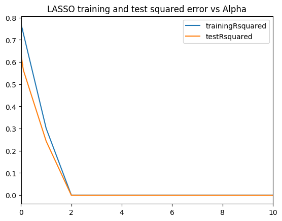
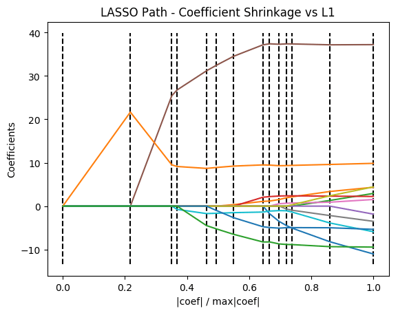
The plot below shows how the 13 coefficients for the 13 predictors vary when lambda is increased. The x-axis includes log (lambda). We can see that increasing lambda from $10^{2}$ to $10^{6}$ significantly shrinks the coefficients. We can draw a vertical line from the x-axis and read the values of the 13 coefficients. Some of them will be close to zero

# Compute the cross validation error
cvRidge=cv.glmnet(X,y,alpha=0)

#Plot the cross validation error
plot(cvRidge, main="Ridge regression Cross Validation Error (10 fold)")

This gives the 10 fold Cross Validation Error with respect to log (lambda) As lambda increase the MSE increases

1.4a Ridge Regression – Python code

The coefficient shrinkage for Python can be plotted like R using Least Angle Regression model a.k.a. LARS package. This is included below

import numpy as np
import pandas as pd
import os
import matplotlib.pyplot as plt
from sklearn.model_selection import train_test_split


df = pd.read_csv("Boston.csv",encoding = "ISO-8859-1")
#Rename the columns
df.columns=["no","crimeRate","zone","indus","chasRiver","NO2","rooms","age",
              "distances","idxHighways","taxRate","teacherRatio","color","status","cost"]
X=df[["crimeRate","zone","indus","chasRiver","NO2","rooms","age",
              "distances","idxHighways","taxRate","teacherRatio","color","status"]]
y=df['cost']
from sklearn.preprocessing import MinMaxScaler
scaler = MinMaxScaler()

from sklearn.linear_model import Ridge
X_train, X_test, y_train, y_test = train_test_split(X, y,
                                                   random_state = 0)

# Scale the X_train and X_test
X_train_scaled = scaler.fit_transform(X_train)
X_test_scaled = scaler.transform(X_test)

# Fit a ridge regression with alpha=20
linridge = Ridge(alpha=20.0).fit(X_train_scaled, y_train)

# Print the training R squared
print('R-squared score (training): {:.3f}'
     .format(linridge.score(X_train_scaled, y_train)))
# Print the test Rsquared
print('R-squared score (test): {:.3f}'
     .format(linridge.score(X_test_scaled, y_test)))
print('Number of non-zero features: {}'
     .format(np.sum(linridge.coef_ != 0)))

trainingRsquared=[]
testRsquared=[]
# Plot the effect of alpha on the test Rsquared
print('Ridge regression: effect of alpha regularization parameter\n')
# Choose a list of alpha values
for this_alpha in [0.001,.01,.1,0, 1, 10, 20, 50, 100, 1000]:
    linridge = Ridge(alpha = this_alpha).fit(X_train_scaled, y_train)
    # Compute training rsquared
    r2_train = linridge.score(X_train_scaled, y_train)
    # Compute test rsqaured
    r2_test = linridge.score(X_test_scaled, y_test)
    num_coeff_bigger = np.sum(abs(linridge.coef_) > 1.0)
    trainingRsquared.append(r2_train)
    testRsquared.append(r2_test)
    
# Create a dataframe
alpha=[0.001,.01,.1,0, 1, 10, 20, 50, 100, 1000]    
trainingRsquared=pd.DataFrame(trainingRsquared,index=alpha)
testRsquared=pd.DataFrame(testRsquared,index=alpha)

# Plot training and test R squared as a function of alpha
df3=pd.concat([trainingRsquared,testRsquared],axis=1)
df3.columns=['trainingRsquared','testRsquared']

fig5=df3.plot()
fig5=plt.title('Ridge training and test squared error vs Alpha')
fig5.figure.savefig('fig5.png', bbox_inches='tight')

# Plot the coefficient shrinage using the LARS package

from sklearn import linear_model
# #############################################################################
# Compute paths

n_alphas = 200
alphas = np.logspace(0, 8, n_alphas)

coefs = []
for a in alphas:
    ridge = linear_model.Ridge(alpha=a, fit_intercept=False)
    ridge.fit(X_train_scaled, y_train)
    coefs.append(ridge.coef_)

# #############################################################################
# Display results

ax = plt.gca()

fig6=ax.plot(alphas, coefs)
fig6=ax.set_xscale('log')
fig6=ax.set_xlim(ax.get_xlim()[::-1])  # reverse axis
fig6=plt.xlabel('alpha')
fig6=plt.ylabel('weights')
fig6=plt.title('Ridge coefficients as a function of the regularization')
fig6=plt.axis('tight')
plt.savefig('fig6.png', bbox_inches='tight')

## R-squared score (training): 0.620
## R-squared score (test): 0.438
## Number of non-zero features: 13
## Ridge regression: effect of alpha regularization parameter

The plot below shows the training and test error when increasing the tuning or regularization parameter ‘alpha’

For Python the coefficient shrinkage with LARS must be viewed from right to left, where you have increasing alpha. As alpha increases the coefficients shrink to 0.

1.5 Lasso regularization

The Lasso is another form of regularization, also known as L1 regularization. Unlike the Ridge Regression where the coefficients of features which do not influence the target tend to zero, in the lasso regualrization the coefficients become 0. The general form of Lasso is as follows

$\sum_{i=1}^{n} (y_{i} - \beta_{0} - \sum_{j=1}^{p}\beta_jx_{ij})^{2} + \lambda \sum_{j=1}^{p}|\beta|$

1.5a Lasso regularization – R code

library(glmnet)
library(dplyr)
df=read.csv("Boston.csv",stringsAsFactors = FALSE) # Data from MASS - SL
names(df) <-c("no","crimeRate","zone","indus","charles","nox","rooms","age",
              "distances","highways","tax","teacherRatio","color","status","cost")
df1 <- df %>% dplyr::select("crimeRate","zone","indus","charles","nox","rooms","age",
                            "distances","highways","tax","teacherRatio","color","status","cost")

# Set X and y as matrices
X=as.matrix(df1[,1:13])
y=df1$cost

# Fit the lasso model
fitLasso <- glmnet(X,y)
# Plot the coefficient shrinkage as a function of log(lambda)
plot(fitLasso,xvar="lambda",label=TRUE,main="Lasso regularization - Coefficient shrinkage vs log lambda")

The plot below shows that in L1 regularization the coefficients actually become zero with increasing lambda

# Compute the cross validation error (10 fold)
cvLasso=cv.glmnet(X,y,alpha=0)
# Plot the cross validation error
plot(cvLasso)

This gives the MSE for the lasso model

1.5 b Lasso regularization – Python code

import numpy as np
import pandas as pd
import os
import matplotlib.pyplot as plt
from sklearn.model_selection import train_test_split
from sklearn.linear_model import Lasso
from sklearn.preprocessing import MinMaxScaler
from sklearn import linear_model

scaler = MinMaxScaler()
df = pd.read_csv("Boston.csv",encoding = "ISO-8859-1")
#Rename the columns
df.columns=["no","crimeRate","zone","indus","chasRiver","NO2","rooms","age",
              "distances","idxHighways","taxRate","teacherRatio","color","status","cost"]
X=df[["crimeRate","zone","indus","chasRiver","NO2","rooms","age",
              "distances","idxHighways","taxRate","teacherRatio","color","status"]]
y=df['cost']
X_train, X_test, y_train, y_test = train_test_split(X, y,
                                                   random_state = 0)

X_train_scaled = scaler.fit_transform(X_train)
X_test_scaled = scaler.transform(X_test)

linlasso = Lasso(alpha=0.1, max_iter = 10).fit(X_train_scaled, y_train)

print('Non-zero features: {}'
     .format(np.sum(linlasso.coef_ != 0)))
print('R-squared score (training): {:.3f}'
     .format(linlasso.score(X_train_scaled, y_train)))
print('R-squared score (test): {:.3f}\n'
     .format(linlasso.score(X_test_scaled, y_test)))
print('Features with non-zero weight (sorted by absolute magnitude):')

for e in sorted (list(zip(list(X), linlasso.coef_)),
                key = lambda e: -abs(e[1])):
    if e[1] != 0:
        print('\t{}, {:.3f}'.format(e[0], e[1]))
        

print('Lasso regression: effect of alpha regularization\n\
parameter on number of features kept in final model\n')

trainingRsquared=[]
testRsquared=[]
#for alpha in [0.01,0.05,0.1, 1, 2, 3, 5, 10, 20, 50]:
for alpha in [0.01,0.07,0.05, 0.1, 1,2, 3, 5, 10]:
    linlasso = Lasso(alpha, max_iter = 10000).fit(X_train_scaled, y_train)
    r2_train = linlasso.score(X_train_scaled, y_train)
    r2_test = linlasso.score(X_test_scaled, y_test)
    trainingRsquared.append(r2_train)
    testRsquared.append(r2_test)
    
alpha=[0.01,0.07,0.05, 0.1, 1,2, 3, 5, 10]    
#alpha=[0.01,0.05,0.1, 1, 2, 3, 5, 10, 20, 50]
trainingRsquared=pd.DataFrame(trainingRsquared,index=alpha)
testRsquared=pd.DataFrame(testRsquared,index=alpha)

df3=pd.concat([trainingRsquared,testRsquared],axis=1)
df3.columns=['trainingRsquared','testRsquared']

fig7=df3.plot()
fig7=plt.title('LASSO training and test squared error vs Alpha')
fig7.figure.savefig('fig7.png', bbox_inches='tight')

## Non-zero features: 7
## R-squared score (training): 0.726
## R-squared score (test): 0.561
## 
## Features with non-zero weight (sorted by absolute magnitude):
##  status, -18.361
##  rooms, 18.232
##  teacherRatio, -8.628
##  taxRate, -2.045
##  color, 1.888
##  chasRiver, 1.670
##  distances, -0.529
## Lasso regression: effect of alpha regularization
## parameter on number of features kept in final model
## 
## Computing regularization path using the LARS ...
## .C:\Users\Ganesh\ANACON~1\lib\site-packages\sklearn\linear_model\coordinate_descent.py:484: ConvergenceWarning: Objective did not converge. You might want to increase the number of iterations. Fitting data with very small alpha may cause precision problems.
##   ConvergenceWarning)

The plot below gives the training and test R squared error

1.5c Lasso coefficient shrinkage – Python code

To plot the coefficient shrinkage for Lasso the Least Angle Regression model a.k.a. LARS package. This is shown below

import numpy as np
import pandas as pd
import os
import matplotlib.pyplot as plt
from sklearn.model_selection import train_test_split
from sklearn.linear_model import Lasso
from sklearn.preprocessing import MinMaxScaler
from sklearn import linear_model
scaler = MinMaxScaler()
df = pd.read_csv("Boston.csv",encoding = "ISO-8859-1")
#Rename the columns
df.columns=["no","crimeRate","zone","indus","chasRiver","NO2","rooms","age",
              "distances","idxHighways","taxRate","teacherRatio","color","status","cost"]
X=df[["crimeRate","zone","indus","chasRiver","NO2","rooms","age",
              "distances","idxHighways","taxRate","teacherRatio","color","status"]]
y=df['cost']
X_train, X_test, y_train, y_test = train_test_split(X, y,
                                                   random_state = 0)

X_train_scaled = scaler.fit_transform(X_train)
X_test_scaled = scaler.transform(X_test)


print("Computing regularization path using the LARS ...")
alphas, _, coefs = linear_model.lars_path(X_train_scaled, y_train, method='lasso', verbose=True)

xx = np.sum(np.abs(coefs.T), axis=1)
xx /= xx[-1]

fig8=plt.plot(xx, coefs.T)

ymin, ymax = plt.ylim()
fig8=plt.vlines(xx, ymin, ymax, linestyle='dashed')
fig8=plt.xlabel('|coef| / max|coef|')
fig8=plt.ylabel('Coefficients')
fig8=plt.title('LASSO Path - Coefficient Shrinkage vs L1')
fig8=plt.axis('tight')
plt.savefig('fig8.png', bbox_inches='tight')

This plot show the coefficient shrinkage for lasso.

This 3rd part of the series covers the main ‘feature selection’ methods. I hope these posts serve as a quick and useful reference to ML code both for R and Python!

Stay tuned for further updates to this series!

Watch this space!

Practical Machine Learning with R and Python – Part 2

In this 2nd part of the series “Practical Machine Learning with R and Python – Part 2”, I continue where I left off in my first post Practical Machine Learning with R and Python – Part 2. In this post I cover the some classification algorithmns and cross validation. Specifically I touch
-Logistic Regression
-K Nearest Neighbors (KNN) classification
-Leave out one Cross Validation (LOOCV)
-K Fold Cross Validation
in both R and Python.

As in my initial post the algorithms are based on the following courses.

Statistical Learning, Prof Trevor Hastie & Prof Robert Tibesherani, Online Stanford
Applied Machine Learning in Python Prof Kevyn-Collin Thomson, University Of Michigan, Coursera

You can download this R Markdown file along with the data from Github. I hope these posts can be used as a quick reference in R and Python and Machine Learning.I have tried to include the coolest part of either course in this post.

The following classification problem is based on Logistic Regression. The data is an included data set in Scikit-Learn, which I have saved as csv and use it also for R. The fit of a classification Machine Learning Model depends on how correctly classifies the data. There are several measures of testing a model’s classification performance. They are

–Accuracy = TP + TN / (TP + TN + FP + FN) – Fraction of all classes correctly classified
–Precision = TP / (TP + FP) – Fraction of correctly classified positives among those classified as positive
– Recall = TP / (TP + FN) Also known as sensitivity, or True Positive Rate (True positive) – Fraction of correctly classified as positive among all positives in the data
– F1 = 2 * Precision * Recall / (Precision + Recall)

1a. Logistic Regression – R code

The caret and e1071 package is required for using the confusionMatrix call

source("RFunctions.R")
library(dplyr)
library(caret)
library(e1071)

# Read the data (from sklearn)
cancer <- read.csv("cancer.csv")
# Rename the target variable
names(cancer) <- c(seq(1,30),"output")
# Split as training and test sets
train_idx <- trainTestSplit(cancer,trainPercent=75,seed=5)
train <- cancer[train_idx, ]
test <- cancer[-train_idx, ]

# Fit a generalized linear logistic model, 
fit=glm(output~.,family=binomial,data=train,control = list(maxit = 50))

# Predict the output from the model
a=predict(fit,newdata=train,type="response")
# Set response >0.5 as 1 and <=0.5 as 0
b=ifelse(a>0.5,1,0)
# Compute the confusion matrix for training data
confusionMatrix(b,train$output)

## Confusion Matrix and Statistics
## 
##           Reference
## Prediction   0   1
##          0 154   0
##          1   0 272
##                                      
##                Accuracy : 1          
##                  95% CI : (0.9914, 1)
##     No Information Rate : 0.6385     
##     P-Value [Acc > NIR] : < 2.2e-16  
##                                      
##                   Kappa : 1          
##  Mcnemar's Test P-Value : NA         
##                                      
##             Sensitivity : 1.0000     
##             Specificity : 1.0000     
##          Pos Pred Value : 1.0000     
##          Neg Pred Value : 1.0000     
##              Prevalence : 0.3615     
##          Detection Rate : 0.3615     
##    Detection Prevalence : 0.3615     
##       Balanced Accuracy : 1.0000     
##                                      
##        'Positive' Class : 0          
##

m=predict(fit,newdata=test,type="response")
n=ifelse(m>0.5,1,0)
# Compute the confusion matrix for test output
confusionMatrix(n,test$output)

## Confusion Matrix and Statistics
## 
##           Reference
## Prediction  0  1
##          0 52  4
##          1  5 81
##                                           
##                Accuracy : 0.9366          
##                  95% CI : (0.8831, 0.9706)
##     No Information Rate : 0.5986          
##     P-Value [Acc > NIR] : <2e-16          
##                                           
##                   Kappa : 0.8677          
##  Mcnemar's Test P-Value : 1               
##                                           
##             Sensitivity : 0.9123          
##             Specificity : 0.9529          
##          Pos Pred Value : 0.9286          
##          Neg Pred Value : 0.9419          
##              Prevalence : 0.4014          
##          Detection Rate : 0.3662          
##    Detection Prevalence : 0.3944          
##       Balanced Accuracy : 0.9326          
##                                           
##        'Positive' Class : 0               
##

1b. Logistic Regression – Python code

import numpy as np
import pandas as pd
import os
import matplotlib.pyplot as plt
from sklearn.model_selection import train_test_split
from sklearn.linear_model import LogisticRegression
os.chdir("C:\\Users\\Ganesh\\RandPython")
from sklearn.datasets import make_classification, make_blobs

from sklearn.metrics import confusion_matrix
from matplotlib.colors import ListedColormap
from sklearn.datasets import load_breast_cancer
# Load the cancer data
(X_cancer, y_cancer) = load_breast_cancer(return_X_y = True)
X_train, X_test, y_train, y_test = train_test_split(X_cancer, y_cancer,
                                                   random_state = 0)
# Call the Logisitic Regression function
clf = LogisticRegression().fit(X_train, y_train)
fig, subaxes = plt.subplots(1, 1, figsize=(7, 5))
# Fit a model
clf = LogisticRegression().fit(X_train, y_train)

# Compute and print the Accuray scores
print('Accuracy of Logistic regression classifier on training set: {:.2f}'
     .format(clf.score(X_train, y_train)))
print('Accuracy of Logistic regression classifier on test set: {:.2f}'
     .format(clf.score(X_test, y_test)))
y_predicted=clf.predict(X_test)
# Compute and print confusion matrix
confusion = confusion_matrix(y_test, y_predicted)
from sklearn.metrics import accuracy_score, precision_score, recall_score, f1_score
print('Accuracy: {:.2f}'.format(accuracy_score(y_test, y_predicted)))
print('Precision: {:.2f}'.format(precision_score(y_test, y_predicted)))
print('Recall: {:.2f}'.format(recall_score(y_test, y_predicted)))
print('F1: {:.2f}'.format(f1_score(y_test, y_predicted)))

## Accuracy of Logistic regression classifier on training set: 0.96
## Accuracy of Logistic regression classifier on test set: 0.96
## Accuracy: 0.96
## Precision: 0.99
## Recall: 0.94
## F1: 0.97

2. Dummy variables

The following R and Python code show how dummy variables are handled in R and Python. Dummy variables are categorival variables which have to be converted into appropriate values before using them in Machine Learning Model For e.g. if we had currency as ‘dollar’, ‘rupee’ and ‘yen’ then the dummy variable will convert this as
dollar 0 0 0
rupee 0 0 1
yen 0 1 0

2a. Logistic Regression with dummy variables- R code

# Load the dummies library
library(dummies)

df <- read.csv("adult1.csv",stringsAsFactors = FALSE,na.strings = c(""," "," ?"))

# Remove rows which have NA
df1 <- df[complete.cases(df),]
dim(df1)

## [1] 30161    16

# Select specific columns
adult <- df1 %>% dplyr::select(age,occupation,education,educationNum,capitalGain,
                               capital.loss,hours.per.week,native.country,salary)
# Set the dummy data with appropriate values
adult1 <- dummy.data.frame(adult, sep = ".")

#Split as training and test
train_idx <- trainTestSplit(adult1,trainPercent=75,seed=1111)
train <- adult1[train_idx, ]
test <- adult1[-train_idx, ]

# Fit a binomial logistic regression
fit=glm(salary~.,family=binomial,data=train)

# Predict response
a=predict(fit,newdata=train,type="response")

# If response >0.5 then it is a 1 and 0 otherwise
b=ifelse(a>0.5,1,0)
confusionMatrix(b,train$salary)

## Confusion Matrix and Statistics
## 
##           Reference
## Prediction     0     1
##          0 16065  3145
##          1   968  2442
##                                           
##                Accuracy : 0.8182          
##                  95% CI : (0.8131, 0.8232)
##     No Information Rate : 0.753           
##     P-Value [Acc > NIR] : < 2.2e-16       
##                                           
##                   Kappa : 0.4375          
##  Mcnemar's Test P-Value : < 2.2e-16       
##                                           
##             Sensitivity : 0.9432          
##             Specificity : 0.4371          
##          Pos Pred Value : 0.8363          
##          Neg Pred Value : 0.7161          
##              Prevalence : 0.7530          
##          Detection Rate : 0.7102          
##    Detection Prevalence : 0.8492          
##       Balanced Accuracy : 0.6901          
##                                           
##        'Positive' Class : 0               
##

# Compute and display confusion matrix
m=predict(fit,newdata=test,type="response")

## Warning in predict.lm(object, newdata, se.fit, scale = 1, type =
## ifelse(type == : prediction from a rank-deficient fit may be misleading

n=ifelse(m>0.5,1,0)
confusionMatrix(n,test$salary)

## Confusion Matrix and Statistics
## 
##           Reference
## Prediction    0    1
##          0 5263 1099
##          1  357  822
##                                           
##                Accuracy : 0.8069          
##                  95% CI : (0.7978, 0.8158)
##     No Information Rate : 0.7453          
##     P-Value [Acc > NIR] : < 2.2e-16       
##                                           
##                   Kappa : 0.4174          
##  Mcnemar's Test P-Value : < 2.2e-16       
##                                           
##             Sensitivity : 0.9365          
##             Specificity : 0.4279          
##          Pos Pred Value : 0.8273          
##          Neg Pred Value : 0.6972          
##              Prevalence : 0.7453          
##          Detection Rate : 0.6979          
##    Detection Prevalence : 0.8437          
##       Balanced Accuracy : 0.6822          
##                                           
##        'Positive' Class : 0               
##

2b. Logistic Regression with dummy variables- Python code

Pandas has a get_dummies function for handling dummies

import numpy as np
import pandas as pd
import os
import matplotlib.pyplot as plt
from sklearn.model_selection import train_test_split
from sklearn.linear_model import LogisticRegression
from sklearn.metrics import confusion_matrix
from sklearn.metrics import accuracy_score, precision_score, recall_score, f1_score
# Read data
df =pd.read_csv("adult1.csv",encoding="ISO-8859-1",na_values=[""," "," ?"])
# Drop rows with NA
df1=df.dropna()
print(df1.shape)
# Select specific columns
adult = df1[['age','occupation','education','educationNum','capitalGain','capital-loss', 
             'hours-per-week','native-country','salary']]

X=adult[['age','occupation','education','educationNum','capitalGain','capital-loss', 
             'hours-per-week','native-country']]
# Set approporiate values for dummy variables
X_adult=pd.get_dummies(X,columns=['occupation','education','native-country'])
y=adult['salary']

X_adult_train, X_adult_test, y_train, y_test = train_test_split(X_adult, y,
                                                   random_state = 0)
clf = LogisticRegression().fit(X_adult_train, y_train)

# Compute and display Accuracy and Confusion matrix
print('Accuracy of Logistic regression classifier on training set: {:.2f}'
     .format(clf.score(X_adult_train, y_train)))
print('Accuracy of Logistic regression classifier on test set: {:.2f}'
     .format(clf.score(X_adult_test, y_test)))
y_predicted=clf.predict(X_adult_test)
confusion = confusion_matrix(y_test, y_predicted)
print('Accuracy: {:.2f}'.format(accuracy_score(y_test, y_predicted)))
print('Precision: {:.2f}'.format(precision_score(y_test, y_predicted)))
print('Recall: {:.2f}'.format(recall_score(y_test, y_predicted)))
print('F1: {:.2f}'.format(f1_score(y_test, y_predicted)))

## (30161, 16)
## Accuracy of Logistic regression classifier on training set: 0.82
## Accuracy of Logistic regression classifier on test set: 0.81
## Accuracy: 0.81
## Precision: 0.68
## Recall: 0.41
## F1: 0.51

3a – K Nearest Neighbors Classification – R code

The Adult data set is taken from UCI Machine Learning Repository

source("RFunctions.R")
df <- read.csv("adult1.csv",stringsAsFactors = FALSE,na.strings = c(""," "," ?"))
# Remove rows which have NA
df1 <- df[complete.cases(df),]
dim(df1)

## [1] 30161    16

# Select specific columns
adult <- df1 %>% dplyr::select(age,occupation,education,educationNum,capitalGain,
                               capital.loss,hours.per.week,native.country,salary)
# Set dummy variables
adult1 <- dummy.data.frame(adult, sep = ".")

#Split train and test as required by KNN classsification model
train_idx <- trainTestSplit(adult1,trainPercent=75,seed=1111)
train <- adult1[train_idx, ]
test <- adult1[-train_idx, ]
train.X <- train[,1:76]
train.y <- train[,77]
test.X <- test[,1:76]
test.y <- test[,77]

# Fit a model for 1,3,5,10 and 15 neighbors
cMat <- NULL
neighbors <-c(1,3,5,10,15)
for(i in seq_along(neighbors)){
    fit =knn(train.X,test.X,train.y,k=i)
    table(fit,test.y)
    a<-confusionMatrix(fit,test.y)
    cMat[i] <- a$overall[1]
    print(a$overall[1])
}

##  Accuracy 
## 0.7835831 
##  Accuracy 
## 0.8162047 
##  Accuracy 
## 0.8089113 
##  Accuracy 
## 0.8209787 
##  Accuracy 
## 0.8184591

#Plot the Accuracy for each of the KNN models
df <- data.frame(neighbors,Accuracy=cMat)
ggplot(df,aes(x=neighbors,y=Accuracy)) + geom_point() +geom_line(color="blue") +
    xlab("Number of neighbors") + ylab("Accuracy") +
    ggtitle("KNN regression - Accuracy vs Number of Neighors (Unnormalized)")

3b – K Nearest Neighbors Classification – Python code

import numpy as np
import pandas as pd
import os
import matplotlib.pyplot as plt
from sklearn.model_selection import train_test_split
from sklearn.metrics import confusion_matrix
from sklearn.metrics import accuracy_score, precision_score, recall_score, f1_score
from sklearn.neighbors import KNeighborsClassifier
from sklearn.preprocessing import MinMaxScaler

# Read data
df =pd.read_csv("adult1.csv",encoding="ISO-8859-1",na_values=[""," "," ?"])
df1=df.dropna()
print(df1.shape)
# Select specific columns
adult = df1[['age','occupation','education','educationNum','capitalGain','capital-loss', 
             'hours-per-week','native-country','salary']]

X=adult[['age','occupation','education','educationNum','capitalGain','capital-loss', 
             'hours-per-week','native-country']]
             
#Set values for dummy variables
X_adult=pd.get_dummies(X,columns=['occupation','education','native-country'])
y=adult['salary']

X_adult_train, X_adult_test, y_train, y_test = train_test_split(X_adult, y,
                                                   random_state = 0)
                                                   
# KNN classification in Python requires the data to be scaled. 
# Scale the data
scaler = MinMaxScaler()
X_train_scaled = scaler.fit_transform(X_adult_train)
# Apply scaling to test set also
X_test_scaled = scaler.transform(X_adult_test)
# Compute the KNN model for 1,3,5,10 & 15 neighbors
accuracy=[]
neighbors=[1,3,5,10,15]
for i in neighbors:
    knn = KNeighborsClassifier(n_neighbors = i)
    knn.fit(X_train_scaled, y_train)
    accuracy.append(knn.score(X_test_scaled, y_test))
    print('Accuracy test score: {:.3f}'
        .format(knn.score(X_test_scaled, y_test)))

# Plot the models with the Accuracy attained for each of these models    
fig1=plt.plot(neighbors,accuracy)
fig1=plt.title("KNN regression - Accuracy vs Number of neighbors")
fig1=plt.xlabel("Neighbors")
fig1=plt.ylabel("Accuracy")
fig1.figure.savefig('foo1.png', bbox_inches='tight')

## (30161, 16)
## Accuracy test score: 0.749
## Accuracy test score: 0.779
## Accuracy test score: 0.793
## Accuracy test score: 0.804
## Accuracy test score: 0.803

Output image:

4 MPG vs Horsepower

The following scatter plot shows the non-linear relation between mpg and horsepower. This will be used as the data input for computing K Fold Cross Validation Error

4a MPG vs Horsepower scatter plot – R Code

df=read.csv("auto_mpg.csv",stringsAsFactors = FALSE) # Data from UCI
df1 <- as.data.frame(sapply(df,as.numeric))

df2 <- df1 %>% dplyr::select(cylinder,displacement, horsepower,weight, acceleration, year,mpg)
df3 <- df2[complete.cases(df2),]
ggplot(df3,aes(x=horsepower,y=mpg)) + geom_point() + xlab("Horsepower") + 
    ylab("Miles Per gallon") + ggtitle("Miles per Gallon vs Hosrsepower")

4b MPG vs Horsepower scatter plot – Python Code

import numpy as np
import pandas as pd
import os
import matplotlib.pyplot as plt
autoDF =pd.read_csv("auto_mpg.csv",encoding="ISO-8859-1")
autoDF.shape
autoDF.columns
autoDF1=autoDF[['mpg','cylinder','displacement','horsepower','weight','acceleration','year']]
autoDF2 = autoDF1.apply(pd.to_numeric, errors='coerce')
autoDF3=autoDF2.dropna()
autoDF3.shape
#X=autoDF3[['cylinder','displacement','horsepower','weight']]
X=autoDF3[['horsepower']]
y=autoDF3['mpg']

fig11=plt.scatter(X,y)
fig11=plt.title("KNN regression - Accuracy vs Number of neighbors")
fig11=plt.xlabel("Neighbors")
fig11=plt.ylabel("Accuracy")
fig11.figure.savefig('foo11.png', bbox_inches='tight')

5 K Fold Cross Validation

K Fold Cross Validation is a technique in which the data set is divided into K Folds or K partitions. The Machine Learning model is trained on K-1 folds and tested on the Kth fold i.e.
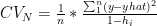
we will have K-1 folds for training data and 1 for testing the ML model. Since we can partition this as $C_{1}^{K}$ or K choose 1, there will be K such partitions. The K Fold Cross
Validation estimates the average validation error that we can expect on a new unseen test data.

The formula for K Fold Cross validation is as follows

$MSE_{K} = \frac{\sum (y-yhat)^{2}}{n_{K}}$
and
$n_{K} = \frac{N}{K}$
and
$CV_{K} = \sum_{K=1}^{K} (\frac{n_{K}}{N}) MSE_{K}$

where $n_{K}$ is the number of elements in partition ‘K’ and N is the total number of elements
$CV_{K} =\sum_{K=1}^{K} MSE_{K}$

$CV_{K} =\frac{\sum_{K=1}^{K} MSE_{K}}{K}$
Leave Out one Cross Validation (LOOCV) is a special case of K Fold Cross Validation where N-1 data points are used to train the model and 1 data point is used to test the model. There are N such paritions of N-1 & 1 that are possible. The mean error is measured The Cross Valifation Error for LOOCV is

$CV_{N} = \frac{1}{n} *\frac{\sum_{1}^{n}(y-yhat)^{2}}{1-h_{i}}$
where $h_{i}$ is the diagonal hat matrix

see [Statistical Learning]

The above formula is also included in this blog post

It took me a day and a half to implement the K Fold Cross Validation formula. I think it is correct. In any case do let me know if you think it is off

5a. Leave out one cross validation (LOOCV) – R Code

R uses the package ‘boot’ for performing Cross Validation error computation

library(boot)
library(reshape2)
# Read data
df=read.csv("auto_mpg.csv",stringsAsFactors = FALSE) # Data from UCI
df1 <- as.data.frame(sapply(df,as.numeric))

# Select complete cases
df2 <- df1 %>% dplyr::select(cylinder,displacement, horsepower,weight, acceleration, year,mpg)
df3 <- df2[complete.cases(df2),]
set.seed(17)
cv.error=rep(0,10)
# For polynomials 1,2,3... 10 fit a LOOCV model
for (i in 1:10){
    glm.fit=glm(mpg~poly(horsepower,i),data=df3)
    cv.error[i]=cv.glm(df3,glm.fit)$delta[1]
    
}
cv.error

##  [1] 24.23151 19.24821 19.33498 19.42443 19.03321 18.97864 18.83305
##  [8] 18.96115 19.06863 19.49093

# Create and display a plot
folds <- seq(1,10)
df <- data.frame(folds,cvError=cv.error)
ggplot(df,aes(x=folds,y=cvError)) + geom_point() +geom_line(color="blue") +
    xlab("Degree of Polynomial") + ylab("Cross Validation Error") +
    ggtitle("Leave one out Cross Validation - Cross Validation Error vs Degree of Polynomial")

5b. Leave out one cross validation (LOOCV) – Python Code

In Python there is no available function to compute Cross Validation error and we have to compute the above formula. I have done this after several hours. I think it is now in reasonable shape. Do let me know if you think otherwise. For LOOCV I use the K Fold Cross Validation with K=N

import numpy as np
import pandas as pd
import os
import matplotlib.pyplot as plt
from sklearn.linear_model import LinearRegression
from sklearn.cross_validation import train_test_split, KFold
from sklearn.preprocessing import PolynomialFeatures
from sklearn.metrics import mean_squared_error
# Read data
autoDF =pd.read_csv("auto_mpg.csv",encoding="ISO-8859-1")
autoDF.shape
autoDF.columns
autoDF1=autoDF[['mpg','cylinder','displacement','horsepower','weight','acceleration','year']]
autoDF2 = autoDF1.apply(pd.to_numeric, errors='coerce')
# Remove rows with NAs
autoDF3=autoDF2.dropna()
autoDF3.shape
X=autoDF3[['horsepower']]
y=autoDF3['mpg']

# For polynomial degree 1,2,3... 10
def computeCVError(X,y,folds):
    deg=[]
    mse=[]
    degree1=[1,2,3,4,5,6,7,8,9,10]
    
    nK=len(X)/float(folds)
    xval_err=0
    # For degree 'j'
    for j in degree1: 
        # Split as 'folds'
        kf = KFold(len(X),n_folds=folds)
        for train_index, test_index in kf:
            # Create the appropriate train and test partitions from the fold index
            X_train, X_test = X.iloc[train_index], X.iloc[test_index]
            y_train, y_test = y.iloc[train_index], y.iloc[test_index]  

            # For the polynomial degree 'j'
            poly = PolynomialFeatures(degree=j)        
            # Transform the X_train and X_test
            X_train_poly = poly.fit_transform(X_train)
            X_test_poly = poly.fit_transform(X_test)
            # Fit a model on the transformed data
            linreg = LinearRegression().fit(X_train_poly, y_train)
            # Compute yhat or ypred
            y_pred = linreg.predict(X_test_poly)   
            # Compute MSE * n_K/N
            test_mse = mean_squared_error(y_test, y_pred)*float(len(X_train))/float(len(X))     
            # Add the test_mse for this partition of the data
            mse.append(test_mse)
        # Compute the mean of all folds for degree 'j'   
        deg.append(np.mean(mse))
        
    return(deg)


df=pd.DataFrame()
print(len(X))
# Call the function once. For LOOCV K=N. hence len(X) is passed as number of folds
cvError=computeCVError(X,y,len(X))

# Create and plot LOOCV
df=pd.DataFrame(cvError)
fig3=df.plot()
fig3=plt.title("Leave one out Cross Validation - Cross Validation Error vs Degree of Polynomial")
fig3=plt.xlabel("Degree of Polynomial")
fig3=plt.ylabel("Cross validation Error")
fig3.figure.savefig('foo3.png', bbox_inches='tight')

6a K Fold Cross Validation – R code

Here K Fold Cross Validation is done for 4, 5 and 10 folds using the R package boot and the glm package

library(boot)
library(reshape2)
set.seed(17)
#Read data
df=read.csv("auto_mpg.csv",stringsAsFactors = FALSE) # Data from UCI
df1 <- as.data.frame(sapply(df,as.numeric))

df2 <- df1 %>% dplyr::select(cylinder,displacement, horsepower,weight, acceleration, year,mpg)
df3 <- df2[complete.cases(df2),]
a=matrix(rep(0,30),nrow=3,ncol=10)
set.seed(17)
# Set the folds as 4,5 and 10
folds<-c(4,5,10)
for(i in seq_along(folds)){
    cv.error.10=rep(0,10)
    for (j in 1:10){
        # Fit a generalized linear model
        glm.fit=glm(mpg~poly(horsepower,j),data=df3)
        # Compute K Fold Validation error
        a[i,j]=cv.glm(df3,glm.fit,K=folds[i])$delta[1]
        
    }
    
}

# Create and display the K Fold Cross Validation Error
b <- t(a)
df <- data.frame(b)
df1 <- cbind(seq(1,10),df)
names(df1) <- c("PolynomialDegree","4-fold","5-fold","10-fold")

df2 <- melt(df1,id="PolynomialDegree")
ggplot(df2) + geom_line(aes(x=PolynomialDegree, y=value, colour=variable),size=2) +
    xlab("Degree of Polynomial") + ylab("Cross Validation Error") +
    ggtitle("K Fold Cross Validation - Cross Validation Error vs Degree of Polynomial")

6b. K Fold Cross Validation – Python code

The implementation of K-Fold Cross Validation Error has to be implemented and I have done this below. There is a small discrepancy in the shapes of the curves with the R plot above. Not sure why!

import numpy as np
import pandas as pd
import os
import matplotlib.pyplot as plt
from sklearn.linear_model import LinearRegression
from sklearn.cross_validation import train_test_split, KFold
from sklearn.preprocessing import PolynomialFeatures
from sklearn.metrics import mean_squared_error
# Read data
autoDF =pd.read_csv("auto_mpg.csv",encoding="ISO-8859-1")
autoDF.shape
autoDF.columns
autoDF1=autoDF[['mpg','cylinder','displacement','horsepower','weight','acceleration','year']]
autoDF2 = autoDF1.apply(pd.to_numeric, errors='coerce')
# Drop NA rows
autoDF3=autoDF2.dropna()
autoDF3.shape
#X=autoDF3[['cylinder','displacement','horsepower','weight']]
X=autoDF3[['horsepower']]
y=autoDF3['mpg']

# Create Cross Validation function
def computeCVError(X,y,folds):
    deg=[]
    mse=[]
    # For degree 1,2,3,..10
    degree1=[1,2,3,4,5,6,7,8,9,10]
    
    nK=len(X)/float(folds)
    xval_err=0
    for j in degree1: 
        # Split the data into 'folds'
        kf = KFold(len(X),n_folds=folds)
        for train_index, test_index in kf:
            # Partition the data acccording the fold indices generated
            X_train, X_test = X.iloc[train_index], X.iloc[test_index]
            y_train, y_test = y.iloc[train_index], y.iloc[test_index]  

            # Scale the X_train and X_test as per the polynomial degree 'j'
            poly = PolynomialFeatures(degree=j)             
            X_train_poly = poly.fit_transform(X_train)
            X_test_poly = poly.fit_transform(X_test)
            # Fit a polynomial regression
            linreg = LinearRegression().fit(X_train_poly, y_train)
            # Compute yhat or ypred
            y_pred = linreg.predict(X_test_poly)  
            # Compute MSE *(nK/N)
            test_mse = mean_squared_error(y_test, y_pred)*float(len(X_train))/float(len(X))  
            # Append to list for different folds
            mse.append(test_mse)
        # Compute the mean for poylnomial 'j' 
        deg.append(np.mean(mse))
        
    return(deg)

# Create and display a plot of K -Folds
df=pd.DataFrame()
for folds in [4,5,10]:
    cvError=computeCVError(X,y,folds)
    #print(cvError)
    df1=pd.DataFrame(cvError)
    df=pd.concat([df,df1],axis=1)
    #print(cvError)
    
df.columns=['4-fold','5-fold','10-fold']
df=df.reindex([1,2,3,4,5,6,7,8,9,10])
df
fig2=df.plot()
fig2=plt.title("K Fold Cross Validation - Cross Validation Error vs Degree of Polynomial")
fig2=plt.xlabel("Degree of Polynomial")
fig2=plt.ylabel("Cross validation Error")
fig2.figure.savefig('foo2.png', bbox_inches='tight')

output

This concludes this 2nd part of this series. I will look into model tuning and model selection in R and Python in the coming parts. Comments, suggestions and corrections are welcome!
To be continued….
Watch this space!

Also see

To see all posts see Index of posts

Practical Machine Learning with R and Python – Part 1

Introduction

This is the 1st part of a series of posts I intend to write on some common Machine Learning Algorithms in R and Python. In this first part I cover the following Machine Learning Algorithms

Univariate Regression
Multivariate Regression
Polynomial Regression
K Nearest Neighbors Regression

The code includes the implementation in both R and Python. This series of posts are based on the following 2 MOOC courses I did at Stanford Online and at Coursera

Statistical Learning, Prof Trevor Hastie & Prof Robert Tibesherani, Online Stanford
Applied Machine Learning in Python Prof Kevyn-Collin Thomson, University Of Michigan, Coursera

I have used the data sets from UCI Machine Learning repository(Communities and Crime and Auto MPG). I also use the Boston data set from MASS package

While coding in R and Python I found that there were some aspects that were more convenient in one language and some in the other. For example, plotting the fit in R is straightforward in R, while computing the R squared, splitting as Train & Test sets etc. are already available in Python. In any case, these minor inconveniences can be easily be implemented in either language.

R squared computation in R is computed as follows
$RSS=\sum (y-yhat)^{2}$
$TSS= \sum(y-mean(y))^{2}$
$Rsquared- 1-\frac{RSS}{TSS}$

Note: You can download this R Markdown file and the associated data sets from Github at MachineLearning-RandPython
Note 1: This post was created as an R Markdown file in RStudio which has a cool feature of including R and Python snippets. The plot of matplotlib needs a workaround but otherwise this is a real cool feature of RStudio!

1.1a Univariate Regression – R code

Here a simple linear regression line is fitted between a single input feature and the target variable

# Source in the R function library
source("RFunctions.R")

# Read the Boston data file
df=read.csv("Boston.csv",stringsAsFactors = FALSE) # Data from MASS - Statistical Learning

# Split the data into training and test sets (75:25)
train_idx <- trainTestSplit(df,trainPercent=75,seed=5)
train <- df[train_idx, ]
test <- df[-train_idx, ]

# Fit a linear regression line between 'Median value of owner occupied homes' vs 'lower status of 
# population'
fit=lm(medv~lstat,data=df)
# Display details of fir
summary(fit)

## 
## Call:
## lm(formula = medv ~ lstat, data = df)
## 
## Residuals:
##     Min      1Q  Median      3Q     Max 
## -15.168  -3.990  -1.318   2.034  24.500 
## 
## Coefficients:
##             Estimate Std. Error t value Pr(>|t|)    
## (Intercept) 34.55384    0.56263   61.41   <2e-16 ***
## lstat       -0.95005    0.03873  -24.53   <2e-16 ***
## ---
## Signif. codes:  0 '***' 0.001 '**' 0.01 '*' 0.05 '.' 0.1 ' ' 1
## 
## Residual standard error: 6.216 on 504 degrees of freedom
## Multiple R-squared:  0.5441, Adjusted R-squared:  0.5432 
## F-statistic: 601.6 on 1 and 504 DF,  p-value: < 2.2e-16

# Display the confidence intervals
confint(fit)

##                 2.5 %     97.5 %
## (Intercept) 33.448457 35.6592247
## lstat       -1.026148 -0.8739505

plot(df$lstat,df$medv, xlab="Lower status (%)",ylab="Median value of owned homes ($1000)", main="Median value of homes ($1000) vs Lowe status (%)")
abline(fit)
abline(fit,lwd=3)
abline(fit,lwd=3,col="red")

rsquared=Rsquared(fit,test,test$medv)
sprintf("R-squared for uni-variate regression (Boston.csv)  is : %f", rsquared)

## [1] "R-squared for uni-variate regression (Boston.csv)  is : 0.556964"

1.1b Univariate Regression – Python code

import numpy as np
import pandas as pd
import os
import matplotlib.pyplot as plt
from sklearn.model_selection import train_test_split
from sklearn.linear_model import LinearRegression
#os.chdir("C:\\software\\machine-learning\\RandPython")

# Read the CSV file
df = pd.read_csv("Boston.csv",encoding = "ISO-8859-1")
# Select the feature variable
X=df['lstat']

# Select the target 
y=df['medv']

# Split into train and test sets (75:25)
X_train, X_test, y_train, y_test = train_test_split(X, y,random_state = 0)
X_train=X_train.values.reshape(-1,1)
X_test=X_test.values.reshape(-1,1)

# Fit a linear model
linreg = LinearRegression().fit(X_train, y_train)

# Print the training and test R squared score
print('R-squared score (training): {:.3f}'.format(linreg.score(X_train, y_train)))
print('R-squared score (test): {:.3f}'.format(linreg.score(X_test, y_test)))
     
# Plot the linear regression line
fig=plt.scatter(X_train,y_train)

# Create a range of points. Compute yhat=coeff1*x + intercept and plot
x=np.linspace(0,40,20)
fig1=plt.plot(x, linreg.coef_ * x + linreg.intercept_, color='red')
fig1=plt.title("Median value of homes ($1000) vs Lowe status (%)")
fig1=plt.xlabel("Lower status (%)")
fig1=plt.ylabel("Median value of owned homes ($1000)")
fig.figure.savefig('foo.png', bbox_inches='tight')
fig1.figure.savefig('foo1.png', bbox_inches='tight')
print "Finished"

## R-squared score (training): 0.571
## R-squared score (test): 0.458
## Finished

1.2a Multivariate Regression – R code

# Read crimes data
crimesDF <- read.csv("crimes.csv",stringsAsFactors = FALSE)

# Remove the 1st 7 columns which do not impact output
crimesDF1 <- crimesDF[,7:length(crimesDF)]

# Convert all to numeric
crimesDF2 <- sapply(crimesDF1,as.numeric)

# Check for NAs
a <- is.na(crimesDF2)
# Set to 0 as an imputation
crimesDF2[a] <-0
#Create as a dataframe
crimesDF2 <- as.data.frame(crimesDF2)
#Create a train/test split
train_idx <- trainTestSplit(crimesDF2,trainPercent=75,seed=5)
train <- crimesDF2[train_idx, ]
test <- crimesDF2[-train_idx, ]

# Fit a multivariate regression model between crimesPerPop and all other features
fit <- lm(ViolentCrimesPerPop~.,data=train)

# Compute and print R Squared
rsquared=Rsquared(fit,test,test$ViolentCrimesPerPop)
sprintf("R-squared for multi-variate regression (crimes.csv)  is : %f", rsquared)

## [1] "R-squared for multi-variate regression (crimes.csv)  is : 0.653940"

1.2b Multivariate Regression – Python code

import numpy as np
import pandas as pd
import os
import matplotlib.pyplot as plt
from sklearn.model_selection import train_test_split
from sklearn.linear_model import LinearRegression
# Read the data
crimesDF =pd.read_csv("crimes.csv",encoding="ISO-8859-1")
#Remove the 1st 7 columns
crimesDF1=crimesDF.iloc[:,7:crimesDF.shape[1]]
# Convert to numeric
crimesDF2 = crimesDF1.apply(pd.to_numeric, errors='coerce')
# Impute NA to 0s
crimesDF2.fillna(0, inplace=True)

# Select the X (feature vatiables - all)
X=crimesDF2.iloc[:,0:120]

# Set the target
y=crimesDF2.iloc[:,121]

X_train, X_test, y_train, y_test = train_test_split(X, y,random_state = 0)
# Fit a multivariate regression model
linreg = LinearRegression().fit(X_train, y_train)

# compute and print the R Square
print('R-squared score (training): {:.3f}'.format(linreg.score(X_train, y_train)))
print('R-squared score (test): {:.3f}'.format(linreg.score(X_test, y_test)))

## R-squared score (training): 0.699
## R-squared score (test): 0.677

1.3a Polynomial Regression – R

For Polynomial regression , polynomials of degree 1,2 & 3 are used and R squared is computed. It can be seen that the quadaratic model provides the best R squared score and hence the best fit

 # Polynomial degree 1
df=read.csv("auto_mpg.csv",stringsAsFactors = FALSE) # Data from UCI
df1 <- as.data.frame(sapply(df,as.numeric))

# Select key columns
df2 <- df1 %>% select(cylinder,displacement, horsepower,weight, acceleration, year,mpg)
df3 <- df2[complete.cases(df2),]

# Split as train and test sets
train_idx <- trainTestSplit(df3,trainPercent=75,seed=5)
train <- df3[train_idx, ]
test <- df3[-train_idx, ]

# Fit a model of degree 1
fit <- lm(mpg~. ,data=train)
rsquared1 <-Rsquared(fit,test,test$mpg)
sprintf("R-squared for Polynomial regression of degree 1 (auto_mpg.csv)  is : %f", rsquared1)

## [1] "R-squared for Polynomial regression of degree 1 (auto_mpg.csv)  is : 0.763607"

# Polynomial degree 2 - Quadratic
x = as.matrix(df3[1:6])
# Make a  polynomial  of degree 2 for feature variables before split
df4=as.data.frame(poly(x,2,raw=TRUE))
df5 <- cbind(df4,df3[7])

# Split into train and test set
train_idx <- trainTestSplit(df5,trainPercent=75,seed=5)
train <- df5[train_idx, ]
test <- df5[-train_idx, ]

# Fit the quadratic model
fit <- lm(mpg~. ,data=train)
# Compute R squared
rsquared2=Rsquared(fit,test,test$mpg)
sprintf("R-squared for Polynomial regression of degree 2 (auto_mpg.csv)  is : %f", rsquared2)

## [1] "R-squared for Polynomial regression of degree 2 (auto_mpg.csv)  is : 0.831372"

#Polynomial degree 3
x = as.matrix(df3[1:6])
# Make polynomial of degree 4  of feature variables before split
df4=as.data.frame(poly(x,3,raw=TRUE))
df5 <- cbind(df4,df3[7])
train_idx <- trainTestSplit(df5,trainPercent=75,seed=5)

train <- df5[train_idx, ]
test <- df5[-train_idx, ]
# Fit a model of degree 3
fit <- lm(mpg~. ,data=train)
# Compute R squared
rsquared3=Rsquared(fit,test,test$mpg)
sprintf("R-squared for Polynomial regression of degree 2 (auto_mpg.csv)  is : %f", rsquared3)

## [1] "R-squared for Polynomial regression of degree 2 (auto_mpg.csv)  is : 0.773225"

df=data.frame(degree=c(1,2,3),Rsquared=c(rsquared1,rsquared2,rsquared3))
# Make a plot of Rsquared and degree
ggplot(df,aes(x=degree,y=Rsquared)) +geom_point() + geom_line(color="blue") +
    ggtitle("Polynomial regression - R squared vs Degree of polynomial") +
    xlab("Degree") + ylab("R squared")

1.3a Polynomial Regression – Python

For Polynomial regression , polynomials of degree 1,2 & 3 are used and R squared is computed. It can be seen that the quadaratic model provides the best R squared score and hence the best fit

import numpy as np
import pandas as pd
import os
import matplotlib.pyplot as plt
from sklearn.model_selection import train_test_split
from sklearn.linear_model import LinearRegression
from sklearn.preprocessing import PolynomialFeatures
autoDF =pd.read_csv("auto_mpg.csv",encoding="ISO-8859-1")
autoDF.shape
autoDF.columns
# Select key columns
autoDF1=autoDF[['mpg','cylinder','displacement','horsepower','weight','acceleration','year']]
# Convert columns to numeric
autoDF2 = autoDF1.apply(pd.to_numeric, errors='coerce')
# Drop NAs
autoDF3=autoDF2.dropna()
autoDF3.shape
X=autoDF3[['cylinder','displacement','horsepower','weight','acceleration','year']]
y=autoDF3['mpg']

# Polynomial degree 1
X_train, X_test, y_train, y_test = train_test_split(X, y,random_state = 0)
linreg = LinearRegression().fit(X_train, y_train)
print('R-squared score - Polynomial degree 1 (training): {:.3f}'.format(linreg.score(X_train, y_train)))
# Compute R squared     
rsquared1 =linreg.score(X_test, y_test)
print('R-squared score - Polynomial degree 1 (test): {:.3f}'.format(linreg.score(X_test, y_test)))

# Polynomial degree 2
poly = PolynomialFeatures(degree=2)
X_poly = poly.fit_transform(X)
X_train, X_test, y_train, y_test = train_test_split(X_poly, y,random_state = 0)
linreg = LinearRegression().fit(X_train, y_train)

# Compute R squared
print('R-squared score - Polynomial degree 2 (training): {:.3f}'.format(linreg.score(X_train, y_train)))
rsquared2 =linreg.score(X_test, y_test)
print('R-squared score - Polynomial degree 2 (test): {:.3f}\n'.format(linreg.score(X_test, y_test)))

#Polynomial degree 3

poly = PolynomialFeatures(degree=3)
X_poly = poly.fit_transform(X)
X_train, X_test, y_train, y_test = train_test_split(X_poly, y,random_state = 0)
linreg = LinearRegression().fit(X_train, y_train)
print('(R-squared score -Polynomial degree 3  (training): {:.3f}'
     .format(linreg.score(X_train, y_train)))
# Compute R squared     
rsquared3 =linreg.score(X_test, y_test)
print('R-squared score Polynomial degree 3 (test): {:.3f}\n'.format(linreg.score(X_test, y_test)))
degree=[1,2,3]
rsquared =[rsquared1,rsquared2,rsquared3]
fig2=plt.plot(degree,rsquared)
fig2=plt.title("Polynomial regression - R squared vs Degree of polynomial")
fig2=plt.xlabel("Degree")
fig2=plt.ylabel("R squared")
fig2.figure.savefig('foo2.png', bbox_inches='tight')
print "Finished plotting and saving"

## R-squared score - Polynomial degree 1 (training): 0.811
## R-squared score - Polynomial degree 1 (test): 0.799
## R-squared score - Polynomial degree 2 (training): 0.861
## R-squared score - Polynomial degree 2 (test): 0.847
## 
## (R-squared score -Polynomial degree 3  (training): 0.933
## R-squared score Polynomial degree 3 (test): 0.710
## 
## Finished plotting and saving

1.4 K Nearest Neighbors

The code below implements KNN Regression both for R and Python. This is done for different neighbors. The R squared is computed in each case. This is repeated after performing feature scaling. It can be seen the model fit is much better after feature scaling. Normalization refers to

$X_{normalized} = \frac{X-min(X)}{max(X-min(X))}$

Another technique that is used is Standardization which is

$X_{standardized} = \frac{X-mean(X)}{sd(X)}$

1.4a K Nearest Neighbors Regression – R( Unnormalized)

The R code below does not use feature scaling

# KNN regression requires the FNN package
df=read.csv("auto_mpg.csv",stringsAsFactors = FALSE) # Data from UCI
df1 <- as.data.frame(sapply(df,as.numeric))

df2 <- df1 %>% select(cylinder,displacement, horsepower,weight, acceleration, year,mpg)
df3 <- df2[complete.cases(df2),]

# Split train and test
train_idx <- trainTestSplit(df3,trainPercent=75,seed=5)
train <- df3[train_idx, ]
test <- df3[-train_idx, ]
#  Select the feature variables
train.X=train[,1:6]
# Set the target for training
train.Y=train[,7]
# Do the same for test set
test.X=test[,1:6]
test.Y=test[,7]

rsquared <- NULL
# Create a list of neighbors
neighbors <-c(1,2,4,8,10,14)
for(i in seq_along(neighbors)){
    # Perform a KNN regression fit
    knn=knn.reg(train.X,test.X,train.Y,k=neighbors[i])
    # Compute R sqaured
    rsquared[i]=knnRSquared(knn$pred,test.Y)
}

# Make a dataframe for plotting
df <- data.frame(neighbors,Rsquared=rsquared)
# Plot the number of neighors vs the R squared
ggplot(df,aes(x=neighbors,y=Rsquared)) + geom_point() +geom_line(color="blue") +
    xlab("Number of neighbors") + ylab("R squared") +
    ggtitle("KNN regression - R squared vs Number of Neighors (Unnormalized)")

1.4b K Nearest Neighbors Regression – Python( Unnormalized)

The Python code below does not use feature scaling

import numpy as np
import pandas as pd
import os
import matplotlib.pyplot as plt
from sklearn.model_selection import train_test_split
from sklearn.linear_model import LinearRegression
from sklearn.preprocessing import PolynomialFeatures
from sklearn.neighbors import KNeighborsRegressor
autoDF =pd.read_csv("auto_mpg.csv",encoding="ISO-8859-1")
autoDF.shape
autoDF.columns
autoDF1=autoDF[['mpg','cylinder','displacement','horsepower','weight','acceleration','year']]
autoDF2 = autoDF1.apply(pd.to_numeric, errors='coerce')
autoDF3=autoDF2.dropna()
autoDF3.shape
X=autoDF3[['cylinder','displacement','horsepower','weight','acceleration','year']]
y=autoDF3['mpg']

# Perform a train/test split
X_train, X_test, y_train, y_test = train_test_split(X, y, random_state = 0)
# Create a list of neighbors
rsquared=[]
neighbors=[1,2,4,8,10,14]
for i in neighbors:
        # Fit a KNN model
        knnreg = KNeighborsRegressor(n_neighbors = i).fit(X_train, y_train)
        # Compute R squared
        rsquared.append(knnreg.score(X_test, y_test))
        print('R-squared test score: {:.3f}'
        .format(knnreg.score(X_test, y_test)))
# Plot the number of neighors vs the R squared        
fig3=plt.plot(neighbors,rsquared)
fig3=plt.title("KNN regression - R squared vs Number of neighbors(Unnormalized)")
fig3=plt.xlabel("Neighbors")
fig3=plt.ylabel("R squared")
fig3.figure.savefig('foo3.png', bbox_inches='tight')
print "Finished plotting and saving"

## R-squared test score: 0.527
## R-squared test score: 0.678
## R-squared test score: 0.707
## R-squared test score: 0.684
## R-squared test score: 0.683
## R-squared test score: 0.670
## Finished plotting and saving

1.4c K Nearest Neighbors Regression – R( Normalized)

It can be seen that R squared improves when the features are normalized.

df=read.csv("auto_mpg.csv",stringsAsFactors = FALSE) # Data from UCI
df1 <- as.data.frame(sapply(df,as.numeric))

df2 <- df1 %>% select(cylinder,displacement, horsepower,weight, acceleration, year,mpg)
df3 <- df2[complete.cases(df2),]

# Perform MinMaxScaling of feature variables 
train.X.scaled=MinMaxScaler(train.X)
test.X.scaled=MinMaxScaler(test.X)

# Create a list of neighbors
rsquared <- NULL
neighbors <-c(1,2,4,6,8,10,12,15,20,25,30)
for(i in seq_along(neighbors)){
    # Fit a KNN model
    knn=knn.reg(train.X.scaled,test.X.scaled,train.Y,k=i)
    # Compute R ssquared
    rsquared[i]=knnRSquared(knn$pred,test.Y)
    
}

df <- data.frame(neighbors,Rsquared=rsquared)
# Plot the number of neighors vs the R squared 
ggplot(df,aes(x=neighbors,y=Rsquared)) + geom_point() +geom_line(color="blue") +
    xlab("Number of neighbors") + ylab("R squared") +
    ggtitle("KNN regression - R squared vs Number of Neighors(Normalized)")

1.4d K Nearest Neighbors Regression – Python( Normalized)

R squared improves when the features are normalized with MinMaxScaling

import numpy as np
import pandas as pd
import os
import matplotlib.pyplot as plt
from sklearn.model_selection import train_test_split
from sklearn.linear_model import LinearRegression
from sklearn.preprocessing import PolynomialFeatures
from sklearn.neighbors import KNeighborsRegressor
from sklearn.preprocessing import MinMaxScaler
autoDF =pd.read_csv("auto_mpg.csv",encoding="ISO-8859-1")
autoDF.shape
autoDF.columns
autoDF1=autoDF[['mpg','cylinder','displacement','horsepower','weight','acceleration','year']]
autoDF2 = autoDF1.apply(pd.to_numeric, errors='coerce')
autoDF3=autoDF2.dropna()
autoDF3.shape
X=autoDF3[['cylinder','displacement','horsepower','weight','acceleration','year']]
y=autoDF3['mpg']

# Perform a train/ test  split
X_train, X_test, y_train, y_test = train_test_split(X, y, random_state = 0)
# Use MinMaxScaling
scaler = MinMaxScaler()
X_train_scaled = scaler.fit_transform(X_train)
# Apply scaling on test set
X_test_scaled = scaler.transform(X_test)

# Create a list of neighbors
rsquared=[]
neighbors=[1,2,4,6,8,10,12,15,20,25,30]
for i in neighbors:
    # Fit a KNN model
    knnreg = KNeighborsRegressor(n_neighbors = i).fit(X_train_scaled, y_train)
    # Compute R squared
    rsquared.append(knnreg.score(X_test_scaled, y_test))
    print('R-squared test score: {:.3f}'
        .format(knnreg.score(X_test_scaled, y_test)))

# Plot the number of neighors vs the R squared 
fig4=plt.plot(neighbors,rsquared)
fig4=plt.title("KNN regression - R squared vs Number of neighbors(Normalized)")
fig4=plt.xlabel("Neighbors")
fig4=plt.ylabel("R squared")
fig4.figure.savefig('foo4.png', bbox_inches='tight')
print "Finished plotting and saving"

## R-squared test score: 0.703
## R-squared test score: 0.810
## R-squared test score: 0.830
## R-squared test score: 0.838
## R-squared test score: 0.834
## R-squared test score: 0.828
## R-squared test score: 0.827
## R-squared test score: 0.826
## R-squared test score: 0.816
## R-squared test score: 0.815
## R-squared test score: 0.809
## Finished plotting and saving

Conclusion

In this initial post I cover the regression models when the output is continous. I intend to touch upon other Machine Learning algorithms.
Comments, suggestions and corrections are welcome.

Watch this this space!

To be continued….

To see all posts see Index of posts

My travels through the realms of Data Science, Machine Learning, Deep Learning and (AI)

Then felt I like some watcher of the skies

When a new planet swims into his ken;

Or like stout Cortez when with eagle eyes

He star’d at the Pacific—and all his men

Look’d at each other with a wild surmise—

Silent, upon a peak in Darien.

On First Looking into Chapman’s Homer by John Keats

The above excerpt from John Keat’s poem captures the the exhilaration that one experiences, when discovering something for the first time. This also summarizes to some extent my own as enjoyment while pursuing Data Science, Machine Learning and the like.

I decided to write this post, as occasionally youngsters approach me and ask me where they should start their adventure in Data Science & Machine Learning. There are other times, when the ‘not-so-youngsters’ want to know what their next step should be after having done some courses. This post includes my travels through the domains of Data Science, Machine Learning, Deep Learning and (soon to be done AI).

By no means, am I an authority in this field, which is ever-widening and almost bottomless, yet I would like to share some of my experiences in this fascinating field. I include a short review of the courses I have done below. I also include alternative routes through courses which I did not do, but are probably equally good as well. Feel free to pick and choose any course or set of courses. Alternatively, you may prefer to read books or attend bricks-n-mortar classes, In any case, I hope the list below will provide you with some overall direction.

All my learning in the above domains have come from MOOCs and I restrict myself to the top 3 MOOCs, or in my opinion, ‘the original MOOCs’, namely Coursera, edX or Udacity, but may throw in some courses from other online sites if they are only available there. I would recommend these 3 MOOCs over the other numerous online courses and also over face-to-face classroom courses for the following reasons. These MOOCs

Are taken by world class colleges and the lectures are delivered by top class Professors who have a great depth of knowledge and a wealth of experience
The Professors, besides delivering quality content, also point out to important tips, tricks and traps
You can revisit lectures in online courses anytime to refresh your memory
Lectures are usually short between 8 -15 mins (Personally, my attention span is around 15-20 mins at a time!)

Here is a fair warning and something quite obvious. No amount of courses, lectures or books will help if you don’t put it to use through some language like Octave, R or Python.

The journey
My trip through Data Science, Machine Learning started with an off-chance remark,about 3 years ago, from an old friend of mine who spoke to me about having done a few courses at Coursera, and really liked it. He further suggested that I should try. This was the final push which set me sailing into this vast domain.

I have included the list of the courses I have done over the past 5 years (37+ certifications completed and another 9 audited-listened only without doing the assignments). For each of the courses I have included a short review of the course, whether I think the course is mandatory, the language in which the course is based on, and finally whether I have done the course myself etc. I have also included alternative courses, which I may have not done, but which I think are equally good. Finally, I suggest some courses which I have heard of and which are very good and worth taking.

1. Machine Learning, Stanford, Prof Andrew Ng, Coursera
(Requirement: Mandatory, Language:Octave,Status:Completed)
This course provides an excellent foundation to build your Machine Learning citadel on. The course covers the mathematical details of linear, logistic and multivariate regression. There is also a good coverage of topics like Neural Networks, SVMs, Anamoly Detection, underfitting, overfitting, regularization etc. Prof Andrew Ng presents the material in a very lucid manner. It is a great course to start with. It would be a good idea to brush up some basics of linear algebra, matrices and a little bit of calculus, specifically computing the local maxima/minima. You should be able to take this course even if you don’t know Octave as the Prof goes over the key aspects of the language.

2. Statistical Learning, Prof Trevor Hastie & Prof Robert Tibesherani, Online Stanford– (Requirement:Mandatory, Language:R, Status;Completed) –
The course includes linear and polynomial regression, logistic regression. Details also include cross-validation and the bootstrap methods, how to do model selection and regularization (ridge and lasso). It also touches on non-linear models, generalized additive models, boosting and SVMs. Some unsupervised learning methods are also discussed. The 2 Professors take turns in delivering lectures with a slight touch of humor.

3a. Data Science Specialization: Prof Roger Peng, Prof Brian Caffo & Prof Jeff Leek, John Hopkins University (Requirement: Option A, Language: R Status: Completed)
This is a comprehensive 10 module specialization based on R. This Specialization gives a very broad overview of Data Science and Machine Learning. The modules cover R programming, Statistical Inference, Practical Machine Learning, how to build R products and R packages and finally has a very good Capstone project on NLP

3b. Applied Data Science with Python Specialization: University of Michigan (Requirement: Option B, Language: Python, Status: Not done)
In this specialization I only did the Applied Machine Learning in Python (Prof Kevyn-Collin Thomson). This is a very good course that covers a lot of Machine Learning algorithms(linear, logistic, ridge, lasso regression, knn, SVMs etc. Also included are confusion matrices, ROC curves etc. This is based on Python’s Scikit Learn

3c. Machine Learning Specialization, University Of Washington (Requirement:Option C, Language:Python, Status : Not completed). This appears to be a very good Specialization in Python

4. Statistics with R Specialization, Duke University (Requirement: Useful and a must know, Language R, Status:Not Completed)
I audited (listened only) to the following 2 modules from this Specialization.
a.Inferential Statistics
b.Linear Regression and Modeling
Both these courses are taught by Prof Mine Cetikya-Rundel who delivers her lessons with extraordinary clarity. Her lectures are filled with many examples which she walks you through in great detail

5.Bayesian Statistics: From Concept to Data Analysis: Univ of California, Santa Cruz (Requirement: Optional, Language : R, Status:Completed)
This is an interesting course and provides an alternative point of view to frequentist approach

6. Data Science and Engineering with Spark, University of California, Berkeley, Prof Antony Joseph, Prof Ameet Talwalkar, Prof Jon Bates
(Required: Mandatory for Big Data, Status:Completed, Language; pySpark)
This specialization contains 3 modules
a.Introduction to Apache Spark
b.Distributed Machine Learning with Apache Spark
c.Big Data Analysis with Apache Spark

This is an excellent course for those who want to make an entry into Distributed Machine Learning. The exercises are fairly challenging and your code will predominantly be made of map/reduce and lambda operations as you process data that is distributed across Spark RDDs. I really liked the part where the Prof shows how a matrix multiplication on a single machine is of the order of O(nd^2+d^3) (which is the basis of Machine Learning) is reduced to O(nd^2) by taking outer products on data which is distributed.

7. Deep Learning Prof Andrew Ng, Younes Bensouda Mourri, Kian Katanforoosh : Requirement:Mandatory,Language:Python, Tensorflow Status:Completed)

This course had 5 Modules which start from the fundamentals of Neural Networks, their derivation and vectorized Python implementation. The specialization also covers regularization, optimization techniques, mini batch normalization, Convolutional Neural Networks, Recurrent Neural Networks, LSTMs applied to a wide variety of real world problems

The modules are
a. Neural Networks and Deep Learning
In this course Prof Andrew Ng explains differential calculus, linear algebra and vectorized Python implementations of Deep Learning algorithms. The derivation for back-propagation is done and then the Prof shows how to compute a multi-layered DL network
b.Improving Deep Neural Networks: Hyperparameter tuning, Regularization and Optimization
Deep Neural Networks can be very flexible, and come with a lots of knobs (hyper-parameters) to tune with. In this module, Prof Andrew Ng shows a systematic way to tune hyperparameters and by how much should one tune. The course also covers regularization(L1,L2,dropout), gradient descent optimization and batch normalization methods. The visualizations used to explain the momentum method, RMSprop, Adam,LR decay and batch normalization are really powerful and serve to clarify the concepts. As an added bonus,the module also includes a great introduction to Tensorflow.
c.Structuring Machine Learning Projects
A very good module with useful tips, tricks and traps that need to be considered while working on Machine Learning and Deep Learning projects
d. Convolutional Neural Networks
This domain has a lot of really cool ideas, where images represented as 3D volumes, are compressed and stretched longitudinally before applying a multi-layered deep learning neural network to this thin slice for performing classification,detection etc. The Prof provides a glimpse into this fascinating world of image classification, detection andl neural art transfer with frameworks like Keras and Tensorflow.
e. Sequence Models
In this module covers in good detail concepts like RNNs, GRUs, LSTMs, word embeddings, beam search and attention model.

8. Neural Networks for Machine Learning, Prof Geoffrey Hinton,University of Toronto
(Requirement: Mandatory, Language;Octave, Status:Completed)
This is a broad course which starts from the basic of Perceptrons, all the way to Boltzman Machines, RNNs, CNNS, LSTMs etc The course also covers regularisation, learning rate decay, momentum method etc

9.Probabilistic Graphical Models, Stanford Prof Daphne Koller(Language:Octave, Status: Partially completed)
This has 3 courses
a.Probabilistic Graphical Models 1: Representation – Done
b.Probabilistic Graphical Models 2: Inference – To do
c.Probabilistic Graphical Models 3: Learning – To do
This course discusses how a system, which can be represented as a complex interaction
of probability distributions, will behave. This is probably the toughest course I did. I did manage to get through the 1st module, While I felt that grasped a few things, I did not wholly understand the import of this. However I feel this is an important domain and I will definitely revisit this in future

10. Reinforcement Specialization : University of Alberta, Prof Adam White and Prof Martha White
(Requirement: Very important, Language;Python, Status: Partially Completed)
This is a set of 4 courses. I did the first 2 of the 4. Reinforcement Learning appears deceptively simple, but it is anything but simple. Definitely a very critical area to learn.

a.Fundamentals of Reinforcement Learning: This course discusses Markov models, value functions and Bellman equations and dynamic programming.
b.Sample based learning Learning methods: This course touches on Monte Carlo methods, Temporal Difference methods, Q Learning etc.

Reinforcement Learning is a must-have in your AI arsenal.

11. Tensorflow in Practice Specialization – Prof Laurence Moroney – Deep Learning.AI
(Requirement: Important, Language;Python, Status: Completed)
This is a good course but definitely do the Deep Learning Specialization by Prof Andrew Ng
There are 4 courses in this Specialization. I completed all 4 courses. They are fairly straight forward
a. Introduction to TensorFlow – This course introduces you to Tensorflow, image recognition with brute-force method
b. Convolutional Neural Networks in Tensorflow – This course touches on how to build a CNN, image augmentation, transfer learning and multi-class classification
c. Natural Language Processing in Tensorflow – Word embeddings, sentiment analysis, LSTMs, RNNs are discussed.
d. Sequences, time series and prediction – This course discusses using RNNs for time series, auto correlation

12. Natural Language Processing Specialization – Prof Younes Bensouda, Lukasz Kaiser from DeepLearning.AI
(Requirement: Very Important, Language;Python, Status: Partially Completed)
This is the latest specialization from Deep Learning.AI. I have completed the first 2 courses
a.Natural Language Processing with Classification and Vector Spaces -The first course deals with sentiment analysis with Naive Bayes, vector space models, capturing dependencies using PCA etc
b. Natural Language Processing with Probabilistic Models – In this course techniques for auto correction, Markov models and Viterbi algorithm for Parts of Speech tagging, auto completion and word embedding are discussed.

13. Mining Massive Data Sets Prof Jure Leskovec, Prof Anand Rajaraman and ProfJeff Ullman. Online Stanford, Status Partially done.,
I did quickly audit this course, a year back, when it used to be in Coursera. It now seems to have moved to Stanford online. But this is a very good course that discusses key concepts of Mining Big Data of the order a few Petabytes

14. Introduction to Artificial Intelligence, Prof Sebastian Thrun & Prof Peter Norvig, Udacity
This is a really good course. I have started on this course a couple of times and somehow gave up. Will revisit to complete in future. Quite extensive in its coverage.Touches BFS,DFS, A-Star, PGM, Machine Learning etc.

15.Deep Learning (with TensorFlow), Vincent Vanhoucke, Principal Scientist at Google Brain.
Got started on this one and abandoned some time back. In my to do list though

16. Generative AI with LLMs

My learning journey is based on Lao Tzu’s dictum of ‘A good traveler has no fixed plans and is not intent on arriving’. You could have a goal and try to plan your courses accordingly.
And so my journey continues…

I hope you find this list useful.
Have a great journey ahead!!!

R vs Python: Different similarities and similar differences

A debate about which language is better suited for Datascience, R or Python, can set off diehard fans of these languages into a tizzy. This post tries to look at some of the different similarities and similar differences between these languages. To a large extent the ease or difficulty in learning R or Python is subjective. I have heard that R has a steeper learning curve than Python and also vice versa. This probably depends on the degree of familiarity with the languuge To a large extent both R an Python do the same thing in just slightly different ways and syntaxes. The ease or the difficulty in the R/Python construct’s largely is in the ‘eyes of the beholder’ nay, programmer’ we could say. I include my own experience with the languages below.

1. R data types

R has the following data types

Character
Integer
Numeric
Logical
Complex
Raw

Python has several data types

Int
float
Long
Complex and so on

2. R Vector vs Python List

A common data type in R is the vector. Python has a similar data type, the list

# R vectors
a<-c(4,5,1,3,4,5)
print(a[3])

## [1] 1

print(a[3:4]) # R does not always need the explicit print.

## [1] 1 3

#R type of variable
print(class(a))

## [1] "numeric"

# Length of a
print(length(a))

## [1] 6

# Python lists
a=[4,5,1,3,4,5] # 
print(a[2]) # Some python IDEs require the explicit print
print(a[2:5])
print(type(a))
# Length of a
print(len(a))

## 1
## [1, 3, 4]
## 
## 6

2a. Other data types – Python

Python also has certain other data types like the tuple, dictionary etc as shown below. R does not have as many of the data types, nevertheless we can do everything that Python does in R

# Python tuple
b = (4,5,7,8)
print(b)


#Python dictionary
c={'name':'Ganesh','age':54,'Work':'Professional'}
print(c)
#Print type of variable c

## (4, 5, 7, 8)
## {'name': 'Ganesh', 'age': 54, 'Work': 'Professional'}

2.Type of Variable

To know the type of the variable in R we use ‘class’, In Python the corresponding command is ‘type’

#R - Type of variable
a<-c(4,5,1,3,4,5)
print(class(a))

## [1] "numeric"

#Python - Print type of tuple a
a=[4,5,1,3,4,5]
print(type(a))
b=(4,3,"the",2)
print(type(b))

## 
##

3. Length

To know length in R, use length()

#R - Length of vector
# Length of a
a<-c(4,5,1,3,4,5)
print(length(a))

## [1] 6

To know the length of a list,tuple or dict we can use len()

# Python - Length of list , tuple etc
# Length of a
a=[4,5,1,3,4,5]
print(len(a))
# Length of b
b = (4,5,7,8)
print(len(b))

## 6
## 4

4. Accessing help

To access help in R we use the ‘?’ or the ‘help’ function

#R - Help - To be done in R console or RStudio
#?sapply
#help(sapply)

Help in python on any topic involves

#Python help - This can be done on a (I)Python console
#help(len)
#?len

5. Subsetting

The key difference between R and Python with regards to subsetting is that in R the index starts at 1. In Python it starts at 0, much like C,C++ or Java To subset a vector in R we use

#R - Subset
a<-c(4,5,1,3,4,8,12,18,1)
print(a[3])

## [1] 1

# To print a range or a slice. Print from the 3rd to the 5th element
print(a[3:6])

## [1] 1 3 4 8

Python also uses indices. The difference in Python is that the index starts from 0/

#Python - Subset
a=[4,5,1,3,4,8,12,18,1]
# Print the 4th element (starts from 0)
print(a[3])

# Print a slice from 4 to 6th element
print(a[3:6])

## 3
## [3, 4, 8]

6. Operations on vectors in R and operation on lists in Python

In R we can do many operations on vectors for e.g. element by element addition, subtraction, exponentation,product etc. as show

#R - Operations on vectors
a<- c(5,2,3,1,7)
b<- c(1,5,4,6,8)

#Element wise Addition
print(a+b)

## [1]  6  7  7  7 15

#Element wise subtraction
print(a-b)

## [1]  4 -3 -1 -5 -1

#Element wise product
print(a*b)

## [1]  5 10 12  6 56

# Exponentiating the elements of a vector
print(a^2)

## [1] 25  4  9  1 49

In Python to do this on lists we need to use the ‘map’ and the ‘lambda’ function as follows

# Python - Operations on list
a =[5,2,3,1,7]
b =[1,5,4,6,8]

#Element wise addition with map & lambda
print(list(map(lambda x,y: x+y,a,b)))
#Element wise subtraction
print(list(map(lambda x,y: x-y,a,b)))
#Element wise product
print(list(map(lambda x,y: x*y,a,b)))
# Exponentiating the elements of a list
print(list(map(lambda x: x**2,a)))

## [6, 7, 7, 7, 15]
## [4, -3, -1, -5, -1]
## [5, 10, 12, 6, 56]
## [25, 4, 9, 1, 49]

However if we create ndarrays from lists then we can do the element wise addition,subtraction,product, etc. like R. Numpy is really a powerful module with many, many functions for matrix manipulations

import numpy as np
a =[5,2,3,1,7]
b =[1,5,4,6,8]
a=np.array(a)
b=np.array(b)
#Element wise addition
print(a+b)
#Element wise subtraction
print(a-b)
#Element wise product
print(a*b)
# Exponentiating the elements of a list
print(a**2)

## [ 6  7  7  7 15]
## [ 4 -3 -1 -5 -1]
## [ 5 10 12  6 56]
## [25  4  9  1 49]

7. Getting the index of element

To determine the index of an element which satisifies a specific logical condition in R use ‘which’. In the code below the index of element which is equal to 1 is 4

# R - Which
a<- c(5,2,3,1,7)
print(which(a == 1))

## [1] 4

In Python array we can use np.where to get the same effect. The index will be 3 as the index starts from 0

# Python - np.where
import numpy as np
a =[5,2,3,1,7]
a=np.array(a)
print(np.where(a==1))

## (array([3], dtype=int64),)

8. Data frames

R, by default comes with a set of in-built datasets. There are some datasets which come with the SkiKit- Learn package

# R 
# To check built datasets use
#data() - In R console or in R Studio
#iris - Don't print to console

We can use the in-built data sets that come with Scikit package

#Python
import sklearn as sklearn
import pandas as pd
from sklearn import datasets
# This creates a Sklearn bunch
data = datasets.load_iris()
# Convert to Pandas dataframe
iris = pd.DataFrame(data.data, columns=data.feature_names)

9. Working with dataframes

With R you can work with dataframes directly. For more complex dataframe operations in R there are convenient packages like dplyr, reshape2 etc. For Python we need to use the Pandas package. Pandas is quite comprehensive in the list of things we can do with data frames The most common operations on a dataframe are

Check the size of the dataframe
Take a look at the top 5 or bottom 5 rows of dataframe
Check the content of the dataframe

a.Size

In R use dim()

#R - Size
dim(iris)

## [1] 150   5

For Python use .shape

#Python - size
import sklearn as sklearn
import pandas as pd
from sklearn import datasets
data = datasets.load_iris()
# Convert to Pandas dataframe
iris = pd.DataFrame(data.data, columns=data.feature_names)
iris.shape

b. Top & bottom 5 rows of dataframe

To know the top and bottom rows of a data frame we use head() & tail as shown below for R and Python

#R 
head(iris,5)

##   Sepal.Length Sepal.Width Petal.Length Petal.Width Species
## 1          5.1         3.5          1.4         0.2  setosa
## 2          4.9         3.0          1.4         0.2  setosa
## 3          4.7         3.2          1.3         0.2  setosa
## 4          4.6         3.1          1.5         0.2  setosa
## 5          5.0         3.6          1.4         0.2  setosa

tail(iris,5)

##     Sepal.Length Sepal.Width Petal.Length Petal.Width   Species
## 146          6.7         3.0          5.2         2.3 virginica
## 147          6.3         2.5          5.0         1.9 virginica
## 148          6.5         3.0          5.2         2.0 virginica
## 149          6.2         3.4          5.4         2.3 virginica
## 150          5.9         3.0          5.1         1.8 virginica

#Python
import sklearn as sklearn
import pandas as pd
from sklearn import datasets
data = datasets.load_iris()
# Convert to Pandas dataframe
iris = pd.DataFrame(data.data, columns=data.feature_names)
print(iris.head(5))
print(iris.tail(5))

##    sepal length (cm)  sepal width (cm)  petal length (cm)  petal width (cm)
## 0                5.1               3.5                1.4               0.2
## 1                4.9               3.0                1.4               0.2
## 2                4.7               3.2                1.3               0.2
## 3                4.6               3.1                1.5               0.2
## 4                5.0               3.6                1.4               0.2
##      sepal length (cm)  sepal width (cm)  petal length (cm)  petal width (cm)
## 145                6.7               3.0                5.2               2.3
## 146                6.3               2.5                5.0               1.9
## 147                6.5               3.0                5.2               2.0
## 148                6.2               3.4                5.4               2.3
## 149                5.9               3.0                5.1               1.8

c. Check the content of the dataframe

#R
summary(iris)

##   Sepal.Length    Sepal.Width     Petal.Length    Petal.Width   
##  Min.   :4.300   Min.   :2.000   Min.   :1.000   Min.   :0.100  
##  1st Qu.:5.100   1st Qu.:2.800   1st Qu.:1.600   1st Qu.:0.300  
##  Median :5.800   Median :3.000   Median :4.350   Median :1.300  
##  Mean   :5.843   Mean   :3.057   Mean   :3.758   Mean   :1.199  
##  3rd Qu.:6.400   3rd Qu.:3.300   3rd Qu.:5.100   3rd Qu.:1.800  
##  Max.   :7.900   Max.   :4.400   Max.   :6.900   Max.   :2.500  
##        Species  
##  setosa    :50  
##  versicolor:50  
##  virginica :50  
##                 
##                 
##

str(iris)

## 'data.frame':    150 obs. of  5 variables:
##  $ Sepal.Length: num  5.1 4.9 4.7 4.6 5 5.4 4.6 5 4.4 4.9 ...
##  $ Sepal.Width : num  3.5 3 3.2 3.1 3.6 3.9 3.4 3.4 2.9 3.1 ...
##  $ Petal.Length: num  1.4 1.4 1.3 1.5 1.4 1.7 1.4 1.5 1.4 1.5 ...
##  $ Petal.Width : num  0.2 0.2 0.2 0.2 0.2 0.4 0.3 0.2 0.2 0.1 ...
##  $ Species     : Factor w/ 3 levels "setosa","versicolor",..: 1 1 1 1 1 1 1 1 1 1 ...

#Python
import sklearn as sklearn
import pandas as pd
from sklearn import datasets
data = datasets.load_iris()
# Convert to Pandas dataframe
iris = pd.DataFrame(data.data, columns=data.feature_names)
print(iris.info())

## 
## RangeIndex: 150 entries, 0 to 149
## Data columns (total 4 columns):
## sepal length (cm)    150 non-null float64
## sepal width (cm)     150 non-null float64
## petal length (cm)    150 non-null float64
## petal width (cm)     150 non-null float64
## dtypes: float64(4)
## memory usage: 4.8 KB
## None

d. Check column names

#R
names(iris)

## [1] "Sepal.Length" "Sepal.Width"  "Petal.Length" "Petal.Width" 
## [5] "Species"

colnames(iris)

## [1] "Sepal.Length" "Sepal.Width"  "Petal.Length" "Petal.Width" 
## [5] "Species"

#Python
import sklearn as sklearn
import pandas as pd
from sklearn import datasets
data = datasets.load_iris()
# Convert to Pandas dataframe
iris = pd.DataFrame(data.data, columns=data.feature_names)
#Get column names
print(iris.columns)

## Index(['sepal length (cm)', 'sepal width (cm)', 'petal length (cm)',
##        'petal width (cm)'],
##       dtype='object')

e. Rename columns

In R we can assign a vector to column names

#R
colnames(iris) <- c("lengthOfSepal","widthOfSepal","lengthOfPetal","widthOfPetal","Species")
colnames(iris)

## [1] "lengthOfSepal" "widthOfSepal"  "lengthOfPetal" "widthOfPetal" 
## [5] "Species"

In Python we can assign a list to s.columns

#Python
import sklearn as sklearn
import pandas as pd
from sklearn import datasets
data = datasets.load_iris()
# Convert to Pandas dataframe
iris = pd.DataFrame(data.data, columns=data.feature_names)
iris.columns = ["lengthOfSepal","widthOfSepal","lengthOfPetal","widthOfPetal"]
print(iris.columns)

## Index(['lengthOfSepal', 'widthOfSepal', 'lengthOfPetal', 'widthOfPetal'], dtype='object')

f.Details of dataframe

#Python
import sklearn as sklearn
import pandas as pd
from sklearn import datasets
data = datasets.load_iris()
# Convert to Pandas dataframe
iris = pd.DataFrame(data.data, columns=data.feature_names)
print(iris.info())

## 
## RangeIndex: 150 entries, 0 to 149
## Data columns (total 4 columns):
## sepal length (cm)    150 non-null float64
## sepal width (cm)     150 non-null float64
## petal length (cm)    150 non-null float64
## petal width (cm)     150 non-null float64
## dtypes: float64(4)
## memory usage: 4.8 KB
## None

g. Subsetting dataframes

# R
#To subset a dataframe 'df' in R we use df[row,column] or df[row vector,column vector]
#df[row,column]
iris[3,4]

## [1] 0.2

#df[row vector, column vector]
iris[2:5,1:3]

##   lengthOfSepal widthOfSepal lengthOfPetal
## 2           4.9          3.0           1.4
## 3           4.7          3.2           1.3
## 4           4.6          3.1           1.5
## 5           5.0          3.6           1.4

#If we omit the row vector, then it implies all rows or if we omit the column vector
# then implies all columns for that row
iris[2:5,]

##   lengthOfSepal widthOfSepal lengthOfPetal widthOfPetal Species
## 2           4.9          3.0           1.4          0.2  setosa
## 3           4.7          3.2           1.3          0.2  setosa
## 4           4.6          3.1           1.5          0.2  setosa
## 5           5.0          3.6           1.4          0.2  setosa

# In R we can all specific columns by column names
iris$Sepal.Length[2:5]

## NULL

#Python
# To select an entire row we use .iloc. The index can be used with the ':'. If 
# .iloc[start row: end row]. If start row is omitted then it implies the beginning of
# data frame, if end row is omitted then it implies all rows till end
#Python
import sklearn as sklearn
import pandas as pd
from sklearn import datasets
data = datasets.load_iris()
# Convert to Pandas dataframe
iris = pd.DataFrame(data.data, columns=data.feature_names)
print(iris.iloc[3])
print(iris[:5])
# In python we can select columns by column name as follows
print(iris['sepal length (cm)'][2:6])
#If you want to select more than 2 columns then you must use the double '[[]]' since the 
# index is a list itself
print(iris[['sepal length (cm)','sepal width (cm)']][4:7])

## sepal length (cm)    4.6
## sepal width (cm)     3.1
## petal length (cm)    1.5
## petal width (cm)     0.2
## Name: 3, dtype: float64
##    sepal length (cm)  sepal width (cm)  petal length (cm)  petal width (cm)
## 0                5.1               3.5                1.4               0.2
## 1                4.9               3.0                1.4               0.2
## 2                4.7               3.2                1.3               0.2
## 3                4.6               3.1                1.5               0.2
## 4                5.0               3.6                1.4               0.2
## 2    4.7
## 3    4.6
## 4    5.0
## 5    5.4
## Name: sepal length (cm), dtype: float64
##    sepal length (cm)  sepal width (cm)
## 4                5.0               3.6
## 5                5.4               3.9
## 6                4.6               3.4

h. Computing Mean, Standard deviation

#R 
#Mean
mean(iris$lengthOfSepal)

## [1] 5.843333

#Standard deviation
sd(iris$widthOfSepal)

## [1] 0.4358663

#Python
#Mean
import sklearn as sklearn
import pandas as pd
from sklearn import datasets
data = datasets.load_iris()
# Convert to Pandas dataframe
iris = pd.DataFrame(data.data, columns=data.feature_names)
# Convert to Pandas dataframe
print(iris['sepal length (cm)'].mean())
#Standard deviation
print(iris['sepal width (cm)'].std())

## 5.843333333333335
## 0.4335943113621737

i. Boxplot

Boxplot can be produced in R using baseplot

#R
boxplot(iris$lengthOfSepal)

Matplotlib is a popular package in Python for plots

#Python
import sklearn as sklearn
import pandas as pd
import matplotlib.pyplot as plt
from sklearn import datasets
data = datasets.load_iris()
# Convert to Pandas dataframe
iris = pd.DataFrame(data.data, columns=data.feature_names)
img=plt.boxplot(iris['sepal length (cm)'])
plt.show(img)

j.Scatter plot

#R
plot(iris$widthOfSepal,iris$lengthOfSepal)

#Python
import matplotlib.pyplot as plt
import sklearn as sklearn
import pandas as pd
from sklearn import datasets
data = datasets.load_iris()
# Convert to Pandas dataframe
iris = pd.DataFrame(data.data, columns=data.feature_names)
img=plt.scatter(iris['sepal width (cm)'],iris['sepal length (cm)'])
#plt.show(img)

k. Read from csv file

#R
tendulkar= read.csv("tendulkar.csv",stringsAsFactors = FALSE,na.strings=c(NA,"-"))
#Dimensions of dataframe
dim(tendulkar)

## [1] 347  13

names(tendulkar)

##  [1] "X"          "Runs"       "Mins"       "BF"         "X4s"       
##  [6] "X6s"        "SR"         "Pos"        "Dismissal"  "Inns"      
## [11] "Opposition" "Ground"     "Start.Date"

Use pandas.read_csv() for Python

#Python
import pandas as pd
#Read csv
tendulkar= pd.read_csv("tendulkar.csv",na_values=["-"])
print(tendulkar.shape)
print(tendulkar.columns)

## (347, 13)
## Index(['Unnamed: 0', 'Runs', 'Mins', 'BF', '4s', '6s', 'SR', 'Pos',
##        'Dismissal', 'Inns', 'Opposition', 'Ground', 'Start Date'],
##       dtype='object')

l. Clean the dataframe in R and Python.

The following steps are done for R and Python
1.Remove rows with ‘DNB’
2.Remove rows with ‘TDNB’
3.Remove rows with absent
4.Remove the “*” indicating not out
5.Remove incomplete rows with NA for R or NaN in Python
6.Do a scatter plot

#R
# Remove rows with 'DNB'
a <- tendulkar$Runs != "DNB"
tendulkar <- tendulkar[a,]
dim(tendulkar)

## [1] 330  13

# Remove rows with 'TDNB'
b <- tendulkar$Runs != "TDNB"
tendulkar <- tendulkar[b,]

# Remove rows with absent
c <- tendulkar$Runs != "absent"
tendulkar <- tendulkar[c,]
dim(tendulkar)

## [1] 329  13

# Remove the "* indicating not out
tendulkar$Runs <- as.numeric(gsub("\\*","",tendulkar$Runs))
dim(tendulkar)

## [1] 329  13

# Select only complete rows - complete.cases()
c <- complete.cases(tendulkar)
#Subset the rows which are complete
tendulkar <- tendulkar[c,]
dim(tendulkar)

## [1] 327  13

# Do some base plotting - Scatter plot
plot(tendulkar$BF,tendulkar$Runs)

#Python 
import pandas as pd
import matplotlib.pyplot as plt
#Read csv
tendulkar= pd.read_csv("tendulkar.csv",na_values=["-"])
print(tendulkar.shape)
# Remove rows with 'DNB'
a=tendulkar.Runs !="DNB"
tendulkar=tendulkar[a]
print(tendulkar.shape)
# Remove rows with 'TDNB'
b=tendulkar.Runs !="TDNB"
tendulkar=tendulkar[b]
print(tendulkar.shape)
# Remove rows with absent
c= tendulkar.Runs != "absent"
tendulkar=tendulkar[c]
print(tendulkar.shape)
# Remove the "* indicating not out
tendulkar.Runs= tendulkar.Runs.str.replace(r"[*]","")
#Select only complete rows - dropna()
tendulkar=tendulkar.dropna()
print(tendulkar.shape)
tendulkar.Runs = tendulkar.Runs.astype(int)
tendulkar.BF = tendulkar.BF.astype(int)
#Scatter plot
plt.scatter(tendulkar.BF,tendulkar.Runs)

## (347, 13)
## (330, 13)
## (329, 13)
## (329, 13)
## (327, 13)

m.Chaining operations on dataframes

To chain a set of operations we need to use an R package like dplyr. Pandas does this The following operations are done on tendulkar data frame by dplyr for R and Pandas for Python below

Group by ground
Compute average runs in each ground
Arrange in descending order

#R
library(dplyr)
tendulkar1 <- tendulkar %>% group_by(Ground) %>% summarise(meanRuns= mean(Runs)) %>%
         arrange(desc(meanRuns))
head(tendulkar1,10)

## # A tibble: 10 × 2
##           Ground  meanRuns
##                 
## 1         Multan 194.00000
## 2          Leeds 193.00000
## 3  Colombo (RPS) 143.00000
## 4        Lucknow 142.00000
## 5          Dhaka 132.75000
## 6     Manchester  93.50000
## 7         Sydney  87.22222
## 8   Bloemfontein  85.00000
## 9     Georgetown  81.00000
## 10 Colombo (SSC)  77.55556

#Python
import pandas as pd
#Read csv
tendulkar= pd.read_csv("tendulkar.csv",na_values=["-"])
print(tendulkar.shape)
# Remove rows with 'DNB'
a=tendulkar.Runs !="DNB"
tendulkar=tendulkar[a]
# Remove rows with 'TDNB'
b=tendulkar.Runs !="TDNB"
tendulkar=tendulkar[b]
# Remove rows with absent
c= tendulkar.Runs != "absent"
tendulkar=tendulkar[c]
# Remove the "* indicating not out
tendulkar.Runs= tendulkar.Runs.str.replace(r"[*]","")

#Select only complete rows - dropna()
tendulkar=tendulkar.dropna()
tendulkar.Runs = tendulkar.Runs.astype(int)
tendulkar.BF = tendulkar.BF.astype(int)
tendulkar1= tendulkar.groupby('Ground').mean()['Runs'].sort_values(ascending=False)
print(tendulkar1.head(10))

## (347, 13)
## Ground
## Multan           194.000000
## Leeds            193.000000
## Colombo (RPS)    143.000000
## Lucknow          142.000000
## Dhaka            132.750000
## Manchester        93.500000
## Sydney            87.222222
## Bloemfontein      85.000000
## Georgetown        81.000000
## Colombo (SSC)     77.555556
## Name: Runs, dtype: float64

9. Functions

product <- function(a,b){
  c<- a*b
  c
}
product(5,7)

## [1] 35

def product(a,b):
  c = a*b
  return c
  
print(product(5,7))

## 35

Conclusion

Personally, I took to R, much like a ‘duck takes to water’. I found the R syntax very simple and mostly intuitive. R packages like dplyr, ggplot2, reshape2, make the language quite irrestible. R is weakly typed and has only numeric and character types as opposed to the full fledged data types in Python.

Python, has too many bells and whistles, which can be a little bewildering to the novice. It is possible that they may be useful as one becomes more experienced with the language. Also I found that installing Python packages sometimes gives errors with Python versions 2.7 or 3.6. This will leave you scrambling to google to find how to fix these problems. These can be quite frustrating. R on the other hand makes installing R packages a breeze.

Anyway, this is my current opinion, and like all opinions, may change in the course of time. Let’s see!

I may write a follow up post with more advanced features of R and Python. So do keep checking! Long live R! Viva la Python!

Note: This post was created using RStudio’s RMarkdown which allows you to embed R and Python code snippets. It works perfectly, except that matplotlib’s pyplot does not display.

Also see
1. My book ‘Deep Learning from first principles:Second Edition’ now on Amazon
2. Dabbling with Wiener filter using OpenCV
3. My book ‘Practical Machine Learning in R and Python: Third edition’ on Amazon
4. Design Principles of Scalable, Distributed Systems
5. Re-introducing cricketr! : An R package to analyze performances of cricketers
6. Natural language processing: What would Shakespeare say?
7. Brewing a potion with Bluemix, PostgreSQL, Node.js in the cloud
8. Simulating an Edge Shape in Android
To see all posts click Index of posts

More book, more cricket! 2nd edition of my books now on Amazon

a) Cricket analytics with cricketr
b) Beaten by sheer pace – Cricket analytics with yorkr
is now available on Amazon, both as Paperback and Kindle versions.

The Kindle versions are just $4.99 for both books. Pick up your copies today!!!

A) Cricket analytics with cricketr: Second Edition

Click here ‘Cricket analytics with cricketr: Second Edition‘

You can download the latest PDF version of the book at ‘Cricket analytics with cricketr and cricpy: Analytics harmony with R and Python-6th edition‘

B) Beaten by sheer pace: Cricket analytics with yorkr(2nd edition)

Click here Beaten by sheer pace! Cricket analytics with yorkr

Pick up your copies today!!!

My 3 video presentations on “Essential R”

In this post I include my 3 video presentations on the topic “Essential R”. In these 3 presentations I cover the entire landscape of R. I cover the following

R Language – The essentials
Key R Packages (dplyr, lubridate, ggplot2, etc.)
How to create R Markdown and share reports
A look at Shiny apps
How to create a simple R package

You can download the relevant slide deck and practice code at Essential R

Essential R – Part 1
This video cover basic R data types – character, numeric, vectors, matrices, lists and data frames. It also touches on how to subset these data types

Essential R – Part 2
This video continues on how to subset dataframes (the most important data type) and some important packages. It also presents one of the most important job of a Data Scientist – that of cleaning and shaping the data. This is done with an example unclean data frame. It also touches on some key operations of dplyr like select, filter, arrange, summarise and mutate. Other packages like lubridate, quantmod are also included. This presentation also shows how to use base plot and ggplot2

Essential R – Part 3
This final session covers R Markdown , and touches on some of the key markdown elements. There is a brief overview of a simple Shiny app. Finally this presentation also shows the key steps to create an R package

These 3 R sessions cover most of the basic R topics that we tend to use in a our day-to-day R way of life. With this you should be able to hit the ground running!

Hope you enjoy these video presentation and also hope you have an even greater time with R!

Check out my 2 books on cricket, a) Cricket analytics with cricketr b) Beaten by sheer pace – Cricket analytics with yorkr, now available in both paperback & kindle versions on Amazon!!! Pick up your copies today!

Also see
1. Introducing QCSimulator: A 5-qubit quantum computing simulator in R
2. Computer Vision: Ramblings on derivatives, histograms and contours
3. Designing a Social Web Portal
4. Revisiting Whats up, Watson – Using Watson’s Question and Answer with Bluemix – Part 2
5. Re-introducing cricketr! : An R package to analyze performances of cricketers

To see all my posts click – Index of posts

cricketr flexes new muscles: The final analysis

Twas brillig, and the slithy toves
Did gyre and gimble in the wabe:
All mimsy were the borogoves,
And the mome raths outgrabe.

       Jabberwocky by Lewis Carroll

No analysis of cricket is complete, without determining how players would perform in the host country. Playing Test cricket on foreign pitches, in the host country, is a ‘real test’ for both batsmen and bowlers. Players, who can perform consistently both on domestic and foreign pitches are the genuinely ‘class’ players. Player performance on foreign pitches lets us differentiate the paper tigers, and home ground bullies among batsmen. Similarly, spinners who perform well, only on rank turners in home ground or pace bowlers who can only swing and generate bounce on specially prepared pitches are neither genuine spinners nor real pace bowlers.

So this post, helps in identifying those with real strengths, and those who play good only when the conditions are in favor, in home grounds. This post brings a certain level of finality to the analysis of players with my R package ‘cricketr’

Besides, I also meant ‘final analysis’ in the literal sense, as I intend to take a long break from cricket analysis/analytics and focus on some other domains like Neural Networks, Deep Learning and Spark.

If you are passionate about cricket, and love analyzing cricket performances, then check out my racy book on cricket ‘Cricket analytics with cricketr and cricpy – Analytics harmony with R & Python’! This book discusses and shows how to use my R package ‘cricketr’ and my Python package ‘cricpy’ to analyze batsmen and bowlers in all formats of the game (Test, ODI and T20). The paperback is available on Amazon at $21.99 and the kindle version at $9.99/Rs 449/-. A must read for any cricket lover! Check it out!!

You can download the latest PDF version of the book at ‘Cricket analytics with cricketr and cricpy: Analytics harmony with R and Python-6th edition‘

Untitled

As already mentioned, my R package ‘cricketr’ uses the statistics info available in ESPN Cricinfo Statsguru. You should be able to install the package from CRAN and use many of the functions available in the package. Please be mindful of ESPN Cricinfo Terms of Use

Important note 1: The latest release of ‘cricketr’ now includes the ability to analyze performances of teams now!! See Cricketr adds team analytics to its repertoire!!!

Important note 2 : Cricketr can now do a more fine-grained analysis of players, see Cricketr learns new tricks : Performs fine-grained analysis of players

Important note 3: Do check out the python avatar of cricketr, ‘cricpy’ in my post ‘Introducing cricpy:A python package to analyze performances of cricketers”

(Note: This page is also hosted at RPubs as cricketrFinalAnalysis. You can download the PDF file at cricketrFinalAnalysis.

Important note: Do check out my other posts using cricketr at cricketr-posts

For getting data of a player against a particular country for the match played in the host country, I just had to add 2 extra parameters to the getPlayerData() function. The cricketr package has been updated with the changed functions for getPlayerData() – Tests, getPlayerDataOD() – ODI and getPlayerDataTT() for the Twenty20s. The updated functions will be available in cricketr Version -0.0.14

The data for the following players have already been obtained with the new, changed getPlayerData() function and have been saved as *.csv files. I will be re-using these files, instead of getting them all over again. Hence the getPlayerData() lines have been commented below

library(cricketr)

1. Performance of a batsman against a host ountry in the host country

For e.g We can the get the data for Sachin Tendulkar for matches played against Australia and in Australia Here opposition=2 and host =2 indicate that the opposition is Australia and the host country is also Australia

#tendulkarAus=getPlayerData(35320,opposition=2,host=2,file="tendulkarVsAusInAus.csv",type="batting")

All cricketr functions can be used with this data frame, as before. All the charts show the performance of Tendulkar in Australia against Australia.

par(mfrow=c(2,3))
par(mar=c(4,4,2,2))
batsman4s("./data/tendulkarVsAusInAus.csv","Tendulkar")
batsman6s("./data/tendulkarVsAusInAus.csv","Tendulkar")
batsmanRunsRanges("./data/tendulkarVsAusInAus.csv","Tendulkar")
batsmanDismissals("./data/tendulkarVsAusInAus.csv","Tendulkar")
batsmanAvgRunsGround("./data/tendulkarVsAusInAus.csv","Tendulkar")
batsmanMovingAverage("./data/tendulkarVsAusInAus.csv","Tendulkar")

dev.off()

## null device 
##           1

2. Relative performances of international batsmen against England in England

While we can analyze the performance of a player against an opposition in some host country, I wanted to compare the relative performances of players, to see how players from different nations play in a host country which is not their home ground.

The following lines gets player’s data of matches played in England and against England.The Oval, Lord’s are famous for generating some dangerous swing and bounce. I chose the following players

Sir Don Bradman (Australia)
Steve Waugh (Australia)
Rahul Dravid (India)
Vivian Richards (West Indies)
Sachin Tendulkar (India)

#tendulkarEng=getPlayerData(35320,opposition=1,host=1,file="tendulkarVsEngInEng.csv",type="batting")
#bradmanEng=getPlayerData(4188,opposition=1,host=1,file="bradmanVsEngInEng.csv",type="batting")
#srwaughEng=getPlayerData(8192,opposition=1,host=1,file="srwaughVsEngInEng.csv",type="batting")
#dravidEng=getPlayerData(28114,opposition=1,host=1,file="dravidVsEngInEng.csv",type="batting")
#vrichardEng=getPlayerData(52812,opposition=1,host=1,file="vrichardsEngInEng.csv",type="batting")

frames <- list("./data/tendulkarVsEngInEng.csv","./data/bradmanVsEngInEng.csv","./data/srwaughVsEngInEng.csv",
               "./data/dravidVsEngInEng.csv","./data/vrichardsEngInEng.csv")
names <- list("S Tendulkar","D Bradman","SR Waugh","R Dravid","Viv Richards")

The Lords and the Oval in England are some of the best pitches in the world. Scoring on these pitches and weather conditions, where there is both swing and bounce really requires excellent batting skills. It can be easily seen that Don Bradman stands heads and shoulders over everybody else, averaging close a cumulative average of 100+. He is followed by Viv Richards, who averages around ~60. Interestingly in English conditions, Rahul Dravid edges out Sachin Tendulkar.

relativeBatsmanCumulativeAvgRuns(frames,names)

# The other 2 plots on relative strike rate and cumulative average strike rate,
shows Viv Richards really  blasts the bowling. Viv Richards has a strike rate 
of 70, while Bradman 62+, followed by Tendulkar.
relativeBatsmanSR(frames,names)

relativeBatsmanCumulativeStrikeRate(frames,names)

3. Relative performances of international batsmen against Australia in Australia

The following players from these countries were chosen

Sachin Tendulkar (India)
Viv Richard (West Indies)
David Gower (England)
Jacques Kallis (South Africa)
Alastair Cook (Emgland)

frames <- list("./data/tendulkarVsAusInAus.csv","./data/vrichardsVAusInAus.csv","./data/dgowerVsAusInAus.csv",
               "./data/kallisVsAusInAus.csv","./data/ancookVsWIInWI.csv")
names <- list("S Tendulkar","Viv Richards","David Gower","J Kallis","AN Cook")

Alastair Cook of England has fantastic cumulative average of 55+ on the pitches of Australia. There is a dip towards the end, but we cannot predict whether it would have continued. AN Cook is followed by Tendulkar who has a steady average of 50+ runs, after which there is Viv Richards.

relativeBatsmanCumulativeAvgRuns(frames,names)

#With respect to cumulative or relative strike rate Viv Richards is a class apart.He seems to really
#tear into bowlers. David Gower has an excellent strike rate and is followed by Tendulkar
relativeBatsmanSR(frames,names)

relativeBatsmanCumulativeStrikeRate(frames,names)

4. Relative performances of international batsmen against India in India

While England & Australia are famous for bouncy tracks with swing, Indian pitches are renowed for being extraordinary turners. Also India has always thrown up world class spinners, from the spin quartet of BS Chandraskehar, Bishen Singh Bedi, EAS Prasanna, S Venkatraghavan, to the times of dangerous Anil Kumble, and now to the more recent Ravichander Ashwon and Harbhajan Singh.

A batsmen who can score runs in India against Indian spinners has to be really adept in handling all kinds of spin.

While Clive Lloyd & Alvin Kallicharan had the best performance against India, they have not been included as ESPN Cricinfo had many of the columns missing.

So I chose the following international players for the analysis against India

Hashim Amla (South Africa)
Alastair Cook (England)
Matthew Hayden (Australia)
Viv Richards (West Indies)

frames <- list("./data/amlaVsIndInInd.csv","./data/ancookVsIndInInd.csv","./data/mhaydenVsIndInInd.csv",
               "./data/vrichardsVsIndInInd.csv")
names <- list("H Amla","AN Cook","M Hayden","Viv Riachards")

Excluding Clive Lloyd & Alvin Kallicharan the next best performer against India is Hashim Amla,followed by Alastair Cook, Viv Richards.

relativeBatsmanCumulativeAvgRuns(frames,names)

#With respect to strike rate, there is no contest when Viv Richards is around. He is clearly the best 
#striker of the ball regardless of whether it is the pacy wickets of 
#Australia/England or the spinning tracks of the subcontinent. After 
#Viv Richards, Hayden and Alastair Cook have good cumulative strike rates
#in India
relativeBatsmanSR(frames,names)

relativeBatsmanCumulativeStrikeRate(frames,names)

5. All time greats of Indian batting

I couldn’t resist checking out how the top Indian batsmen perform when playing in host countries So here is a look at how the top Indian batsmen perform against different host countries

6. Top Indian batsmen against Australia in Australia

The following Indian batsmen were chosen

Sunil Gavaskar
Sachin Tendulkar
Virat Kohli
Virendar Sehwag
VVS Laxman

frames <- list("./data/tendulkarVsAusInAus.csv","./data/gavaskarVsAusInAus.csv","./data/kohliVsAusInAus.csv",
               "./data/sehwagVsAusInAus.csv","./data/vvslaxmanVsAusInAus.csv")
names <- list("S Tendulkar","S Gavaskar","V Kohli","V Sehwag","VVS Laxman")

Virat Kohli has the best overall performance against Australia, with a current cumulative average of 60+ runs for the total number of innings played by him (15). With 15 matches the 2nd best is Virendar Sehwag, followed by VVS Laxman. Tendulkar maintains a cumulative average of 48+ runs for an excess of 30+ innings.

relativeBatsmanCumulativeAvgRuns(frames,names)

# Sehwag leads the strike rate against host Australia, followed by 
# Tendulkar in Australia and then Kohli
relativeBatsmanSR(frames,names)

relativeBatsmanCumulativeStrikeRate(frames,names)

7. Top Indian batsmen against England in England

The top Indian batmen’s performances against England are shown below

Rahul Dravid
Dilip Vengsarkar
Rahul Dravid
Sourav Ganguly
Virat Kohli

frames <- list("./data/tendulkarVsEngInEng.csv","./data/dravidVsEngInEng.csv","./data/vengsarkarVsEngInEng.csv",
               "./data/gangulyVsEngInEng.csv","./data/gavaskarVsEngInEng.csv","./data/kohliVsEngInEng.csv")
names <- list("S Tendulkar","R Dravid","D Vengsarkar","S Ganguly","S Gavaskar","V Kohli")

Rahul Dravid has the best performance against England and edges out Tendulkar. He is followed by Tendulkar and then Sourav Ganguly. Note:Incidentally Virat Kohli’s performance against England in England so far has been extremely poor and he averages around 13-15 runs per innings. However he has a long way to go and I hope he catches up. In any case it will be an uphill climb for Kohli in England.

relativeBatsmanCumulativeAvgRuns(frames,names)

#Tendulkar, Ganguly and Dravid have the best strike rate and in that order.
relativeBatsmanSR(frames,names)

relativeBatsmanCumulativeStrikeRate(frames,names)

8. Top Indian batsmen against West Indies in West Indies

frames <- list("./data/tendulkarVsWInWI.csv","./data/dravidVsWInWI.csv","./data/vvslaxmanVsWIInWI.csv",
               "./data/gavaskarVsWIInWI.csv")
names <- list("S Tendulkar","R Dravid","VVS Laxman","S Gavaskar")

Against the West Indies Sunil Gavaskar is heads and shoulders above the rest. Gavaskar has a very impressive cumulative average against West Indies

relativeBatsmanCumulativeAvgRuns(frames,names)

# VVS Laxman followed by  Tendulkar & then Dravid have a very 
# good strike rate against the West Indies
relativeBatsmanCumulativeStrikeRate(frames,names)

9. World’s best spinners on tracks suited for pace & bounce

In this part I compare the performances of the top 3 spinners in recent years and check out how they perform on surfaces that are known for pace, and bounce. I have taken the following 3 spinners

Anil Kumble (India)
M Muralitharan (Sri Lanka)
Shane Warne (Australia)

#kumbleEng=getPlayerData(30176  ,opposition=3,host=3,file="kumbleVsEngInEng.csv",type="bowling")
#muraliEng=getPlayerData(49636  ,opposition=3,host=3,file="muraliVsEngInEng.csv",type="bowling")
#warneEng=getPlayerData(8166  ,opposition=3,host=3,file="warneVsEngInEng.csv",type="bowling")

10. Top international spinners against England in England

frames <- list("./data/kumbleVsEngInEng.csv","./data/muraliVsEngInEng.csv","./data/warneVsEngInEng.csv")
names <- list("Anil KUmble","M Muralitharan","Shane Warne")

Against England and in England, Muralitharan shines with a cumulative average of nearly 5 wickets per match with a peak of almost 8 wickets. Shane Warne has a steady average at 5 wickets and then Anil Kumble.

relativeBowlerCumulativeAvgWickets(frames,names)

# The order relative cumulative Economy rate, Warne has the best figures,followed by Anil Kumble. Muralitharan
# is much more expensive.
relativeBowlerCumulativeAvgEconRate(frames,names)

11. Top international spinners against South Africa in South Africa

frames <- list("./data/kumbleVsSAInSA.csv","./data/muraliVsSAInSA.csv","./data/warneVsSAInSA.csv")
names <- list("Anil Kumble","M Muralitharan","Shane Warne")

In South Africa too, Muralitharan has the best wicket taking performance averaging about 4 wickets. Warne averages around 3 wickets and Kumble around 2 wickets

relativeBowlerCumulativeAvgWickets(frames,names)

# Muralitharan is expensive in South Africa too, while Kumble and Warne go neck-to-neck in the economy rate.
# Kumble edges out Warne and has a better cumulative average economy rate
relativeBowlerCumulativeAvgEconRate(frames,names)

11. Top international pacers against India in India

As a final analysis I check how the world’s pacers perform in India against India. India pitches are supposed to be flat devoid of bounce, while being terrific turners. Hence Indian pitches are more suited to spin bowling than pace bowling. This is changing these days.

The best performers against India in India are mostly the deadly pacemen of yesteryears

For this I have chosen the following bowlers

Courtney Walsh (West Indies)
Andy Roberts (West Indies)
Malcolm Marshall
Glenn McGrath

#cawalshInd=getPlayerData(53216  ,opposition=6,host=6,file="cawalshVsIndInInd.csv",type="bowling")
#arobertsInd=getPlayerData(52817  ,opposition=6,host=6,file="arobertsIndInInd.csv",type="bowling")
#mmarshallInd=getPlayerData(52419  ,opposition=6,host=6,file="mmarshallVsIndInInd.csv",type="bowling")
#gmccgrathInd=getPlayerData(6565  ,opposition=6,host=6,file="mccgrathVsIndInInd.csv",type="bowling")

frames <- list("./data/cawalshVsIndInInd.csv","./data/arobertsIndInInd.csv","./data/mmarshallVsIndInInd.csv",
               "./data/mccgrathVsIndInInd.csv")
names <- list("C Walsh","A Roberts","M Marshall","G McGrath")

Courtney Walsh has the best performance, followed by Andy Roberts followed by Andy Roberts and then Malcom Marshall who tips ahead of Glenn McGrath

relativeBowlerCumulativeAvgWickets(frames,names)

#On the other hand McGrath has the best economy rate, followed by A Roberts and then Courtney Walsh
relativeBowlerCumulativeAvgEconRate(frames,names)

12. ODI performance of a player against a specific country in the host country

This gets the data for MS Dhoni in ODI matches against Australia and in Australia

#dhoniAusODI=getPlayerDataOD(28081,opposition=2,host=2,file="dhoniVsAusInAusODI.csv",type="batting")

13. Twenty 20 performance of a player against a specific country in the host country

#dhoniAusTT=getPlayerDataOD(28081,opposition=2,host=2,file="dhoniVsAusInAusTT.csv",type="batting")

All the ODI and Twenty20 functions of cricketr can be used on the above dataframes of MS Dhoni.

Some key observations

Here are some key observations

At the top of the batting spectrum is Don Bradman with a very impressive average 100-120 in matches played in England and Australia. Unfortunately there weren’t matches he played in other countries and different pitches. 2.Viv Richard has the best cumulative strike rate overall.
Muralitharan strikes more often than Kumble or Warne even in pitches at ENgland, South Africa and West Indies. However Muralitharan is also the most expensive
Warne and Kumble have a much better economy rate than Muralitharan.
Sunil Gavaskar has an extremely impressive performance in West Indies.
Rahul Dravid performs much better than Tendulkar in both England and West Indies.
Virat Kohli has the best performance against Australia so far and hope he maintains his stellar performance followed by Sehwag. However Kohli’s performance in England has been very poor
West Indies batsmen and bowlers seem to thrive on Indian pitches, with Clive Lloyd and Alvin Kalicharan at the top of the list.

1. Splines

1.1a Fit a 4th degree polynomial – R code

1.1b Fit a 4th degree polynomial – Python code

1.1c Fit a B-Spline – R Code

1.1d Fit a Natural Spline – R Code

1.1.e Fit a Smoothing Spline – R code

1.1e Splines – Python

1.2 Generalized Additiive models (GAMs)

1.2a Generalized Additive Models (GAMs) – R Code

1.2b Generalized Additive Models (GAMs) – Python Code

1.3 Tree based Machine Learning Models

Bagging, Random Forest and Gradient Boosting

1.31a Decision Trees – R Code

1.31b Decision Trees – Cross Validation – R Code

1.31c Decision Trees – Python Code

1.31d Decision Trees – Cross Validation – Python Code

1.4a Random Forest – R code

1.4b Random Forest-OOB and Cross Validation Error – R code

1.4c Random Forest – Python code

1.4d Random Forest – Cross Validation and OOB Error – Python code

1.5a Boosting – R code

1.5b Cross Validation Boosting – R code

1.5c Boosting – Python code

1.5c Cross Validation Boosting – Python code

Rate this:

Share:

1.1a. Linear SVM – R code

1.1b Linear SVM – Python code

1.2 Dummy classifier

1.2a Dummy classifier – R code

1.2b Dummy classifier – Python code

1.3a – Radial SVM (un-normalized) – R code

1.4b – Radial SVM (un-normalized) – Python code

1.5a – Radial SVM (Normalized) -R Code

1.5b – Radial SVM (normalized) – Python

1.6a Validation curve – R code

1.6b Validation curve – Python

1.7a Validation Curve (Preventing data leakage) – Python code

1.8 a Decision trees – R code

1.8 b Decision trees – Python code

1.9a Feature importance – R code

1.9b Feature importance – Python code

1.10a Precision-Recall, ROC curves & AUC- R code

1.10b Precision-Recall, ROC curves & AUC- Python code

1.10c Precision-Recall, ROC curves & AUC- Python code

Conclusion

Rate this:

Share:

1.1a Linear Regression – R code

1.1a Best Fit – R code

1.1b Best fit (Exhaustive Search ) – Python code

1.2 Forward fit

1.2a Forward fit – R code

1.2b Forward fit with Cross Validation – R code

1.2c Forward fit – Python code

1.3 Backward Fit

1.3a Backward fit – R code

1.3b Backward fit – Python code

1.3c Sequential Floating Forward Selection (SFFS) – Python code

1.3d Sequential Floating Backward Selection (SFBS) – Python code

1.4 Ridge regression

1.4a Ridge Regression – R code

1.4a Ridge Regression – Python code

1.5 Lasso regularization

1.5a Lasso regularization – R code

1.5 b Lasso regularization – Python code

1.5c Lasso coefficient shrinkage – Python code

Rate this:

Share:

1a. Logistic Regression – R code

1b. Logistic Regression – Python code

2. Dummy variables

2a. Logistic Regression with dummy variables- R code

2b. Logistic Regression with dummy variables- Python code

3a – K Nearest Neighbors Classification – R code

3b – K Nearest Neighbors Classification – Python code

4 MPG vs Horsepower

4a MPG vs Horsepower scatter plot – R Code

4b MPG vs Horsepower scatter plot – Python Code

5 K Fold Cross Validation