Introducing QCSimulator: A 5-qubit quantum computing simulator in R

Introduction

My 5-qubit Quantum Computing Simulator,QCSimulator, is finally ready, and here it is! I have been able to successfully complete this simulator by working through a fair amount of material. To a large extent, the simulator is easy, if one understands how to solve the quantum circuit. However the theory behind quantum computing itself, is quite formidable, and I hope to scale this mountain over a period of time.

QCSimulator is now on CRAN!!!

The code for the QCSimulator package is also available at Github QCSimulator. This post has also been published at Rpubs as QCSimulator and can be downloaded as a PDF document at QCSimulator.pdf

Disclaimer: This article represents the author’s viewpoint only and doesn’t necessarily represent IBM’s positions, strategies or opinions

install.packages("QCSimulator")
library(QCSimulator)
library(ggplot2)

1. Initialize the environment and set global variables

Here I initialize the environment with global variables and then display a few of them.

rm(list=ls())
#Call the init function to initialize the environment and create global variables
init()

# Display some of global variables in environment
ls()

##  [1] "I16"     "I2"      "I4"      "I8"      "q0_"     "q00_"    "q000_"  
##  [8] "q0000_"  "q00000_" "q00001_" "q0001_"  "q00010_" "q00011_" "q001_"  
## [15] "q0010_"  "q00100_" "q00101_" "q0011_"  "q00110_" "q00111_" "q01_"   
## [22] "q010_"   "q0100_"  "q01000_" "q01001_" "q0101_"  "q01010_" "q01011_"
## [29] "q011_"   "q0110_"  "q01100_" "q01101_" "q0111_"  "q01111_" "q1_"    
## [36] "q10_"    "q100_"   "q1000_"  "q10000_" "q10001_" "q1001_"  "q10010_"
## [43] "q10011_" "q101_"   "q1010_"  "q10100_" "q10101_" "q1011_"  "q10110_"
## [50] "q10111_" "q11_"    "q110_"   "q1100_"  "q11000_" "q11001_" "q1101_" 
## [57] "q11010_" "q11011_" "q111_"   "q1110_"  "q11100_" "q11101_" "q1111_" 
## [64] "q11110_" "q11111_"

#1. 2 x 2 Identity matrix 
I2

##      [,1] [,2]
## [1,]    1    0
## [2,]    0    1

#2. 8 x 8 Identity matrix 
I8

##      [,1] [,2] [,3] [,4] [,5] [,6] [,7] [,8]
## [1,]    1    0    0    0    0    0    0    0
## [2,]    0    1    0    0    0    0    0    0
## [3,]    0    0    1    0    0    0    0    0
## [4,]    0    0    0    1    0    0    0    0
## [5,]    0    0    0    0    1    0    0    0
## [6,]    0    0    0    0    0    1    0    0
## [7,]    0    0    0    0    0    0    1    0
## [8,]    0    0    0    0    0    0    0    1

#3. Qubit |00>
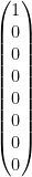
q00_

##      [,1]
## [1,]    1
## [2,]    0
## [3,]    0
## [4,]    0

#4. Qubit |010>
q010_

##      [,1]
## [1,]    0
## [2,]    0
## [3,]    1
## [4,]    0
## [5,]    0
## [6,]    0
## [7,]    0
## [8,]    0

#5. Qubit |0100>
q0100_

##       [,1]
##  [1,]    0
##  [2,]    0
##  [3,]    0
##  [4,]    0
##  [5,]    1
##  [6,]    0
##  [7,]    0
##  [8,]    0
##  [9,]    0
## [10,]    0
## [11,]    0
## [12,]    0
## [13,]    0
## [14,]    0
## [15,]    0
## [16,]    0

#6. Qubit 10010
q10010_

##       [,1]
##  [1,]    0
##  [2,]    0
##  [3,]    0
##  [4,]    0
##  [5,]    0
##  [6,]    0
##  [7,]    0
##  [8,]    0
##  [9,]    0
## [10,]    0
## [11,]    0
## [12,]    0
## [13,]    0
## [14,]    0
## [15,]    0
## [16,]    0
## [17,]    0
## [18,]    0
## [19,]    1
## [20,]    0
## [21,]    0
## [22,]    0
## [23,]    0
## [24,]    0
## [25,]    0
## [26,]    0
## [27,]    0
## [28,]    0
## [29,]    0
## [30,]    0
## [31,]    0
## [32,]    0

The QCSimulator implements the following gates

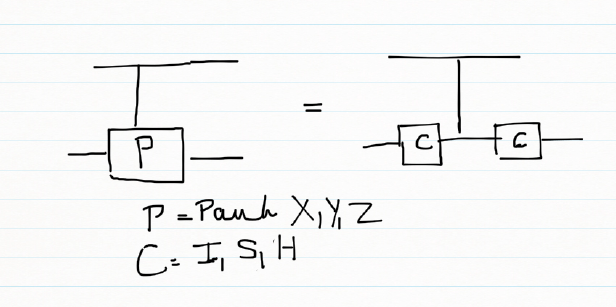
Pauli X,Y,Z, S,S’, T, T’ gates
Rotation , Hadamard,CSWAP,Toffoli gates
2,3,4,5 qubit CNOT gates e.g CNOT2_01,CNOT3_20,CNOT4_13 etc
Toffoli State,SWAPQ0Q1

2. To display the unitary matrix of gates

To check the unitary matrix of gates, we need to pass the appropriate identity matrix as an argument. Hence below the qubit gates require a 2 x 2 unitary matrix and the 2 & 3 qubit CNOT gates require a 4 x 4 and 8 x 8 identity matrix respectively

PauliX(I2)

##      [,1] [,2]
## [1,]    0    1
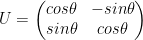
## [2,]    1    0

Hadamard(I2)

##           [,1]       [,2]
## [1,] 0.7071068  0.7071068
## [2,] 0.7071068 -0.7071068

S1Gate(I2)

##      [,1] [,2]
## [1,] 1+0i 0+0i
## [2,] 0+0i 0-1i

CNOT2_10(I4)

##      [,1] [,2] [,3] [,4]
## [1,]    1    0    0    0
## [2,]    0    0    0    1
## [3,]    0    0    1    0
## [4,]    0    1    0    0

CNOT3_20(I8)

##      [,1] [,2] [,3] [,4] [,5] [,6] [,7] [,8]
## [1,]    1    0    0    0    0    0    0    0
## [2,]    0    0    0    0    0    1    0    0
## [3,]    0    0    1    0    0    0    0    0
## [4,]    0    0    0    0    0    0    0    1
## [5,]    0    0    0    0    1    0    0    0
## [6,]    0    1    0    0    0    0    0    0
## [7,]    0    0    0    0    0    0    1    0
## [8,]    0    0    0    1    0    0    0    0

3. Compute the inner product of vectors

For example of phi = 1/2|0> + sqrt(3)/2|1> and si= 1/sqrt(2)(10> + |1>) then the inner product is the dot product of the vectors

phi = matrix(c(1/2,sqrt(3)/2),nrow=2,ncol=1)
si = matrix(c(1/sqrt(2),1/sqrt(2)),nrow=2,ncol=1)
angle= innerProduct(phi,si)
cat("Angle between vectors is:",angle)

## Angle between vectors is: 15

4. Compute the dagger function for a gate

The gate dagger computes and displays the transpose of the complex conjugate of the matrix

TGate(I2)

##      [,1]                 [,2]
## [1,] 1+0i 0.0000000+0.0000000i
## [2,] 0+0i 0.7071068+0.7071068i

GateDagger(TGate(I2))

##      [,1]                 [,2]
## [1,] 1+0i 0.0000000+0.0000000i
## [2,] 0+0i 0.7071068-0.7071068i

5. Invoking gates in series

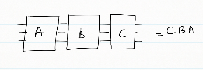
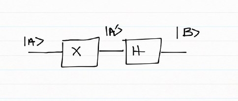
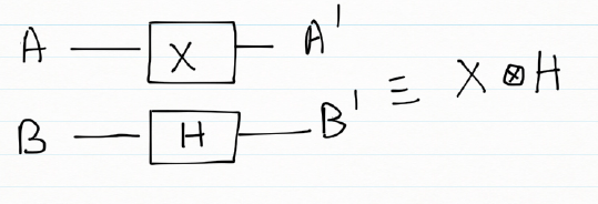
The Quantum gates can be chained by passing each preceding Quantum gate as the argument. The final gate in the chain will have the qubit or the identity matrix passed to it.

# Call in reverse order
# Superposition states
# |+> state
Hadamard(q0_)

##           [,1]
## [1,] 0.7071068
## [2,] 0.7071068

# |-> ==> H x Z 
PauliZ(Hadamard(q0_))

##            [,1]
## [1,]  0.7071068
## [2,] -0.7071068

# (+i) Y ==> H x  S 
 SGate(Hadamard(q0_))

##                      [,1]
## [1,] 0.7071068+0.0000000i
## [2,] 0.0000000+0.7071068i

# (-i)Y ==> H x S1
 S1Gate(Hadamard(q0_))

##                      [,1]
## [1,] 0.7071068+0.0000000i
## [2,] 0.0000000-0.7071068i

# Q1 -- TGate- Hadamard
Q1 = Hadamard(TGate(I2))

6. More gates in series

TGate of depth 2

The Quantum circuit for a TGate of Depth 2 is

Q0 — Hadamard-TGate-Hadamard-TGate-SGate-Measurement as shown in IBM’s Quantum Experience Composer

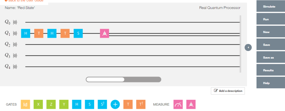
Implementing the quantum gates in series in reverse order we have

# Invoking this in reverse order we get
a = SGate(TGate(Hadamard(TGate(Hadamard(q0_)))))
result=measurement(a)

plotMeasurement(result)

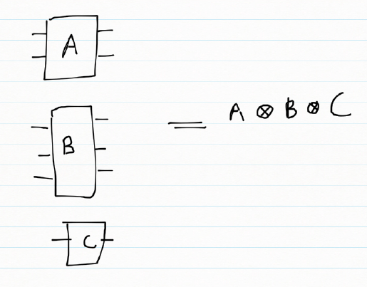
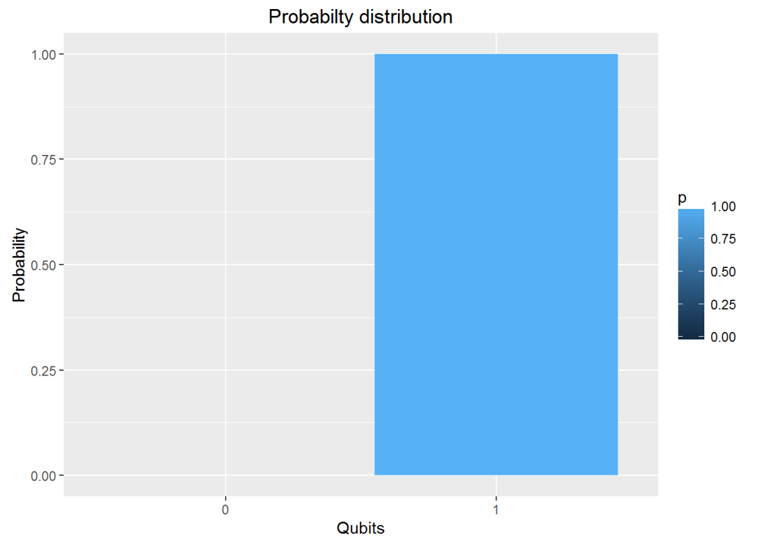
7. Invoking gates in parallel

To obtain the results of gates in parallel we have to take the Tensor Product Note:In the TensorProduct invocation the Identity matrix is passed as an argument to get the unitary matrix of the gate. Q0 – Hadamard-Measurement Q1 – Identity- Measurement

# 
a = TensorProd(Hadamard(I2),I2)
b = DotProduct(a,q00_)
plotMeasurement(measurement(b))

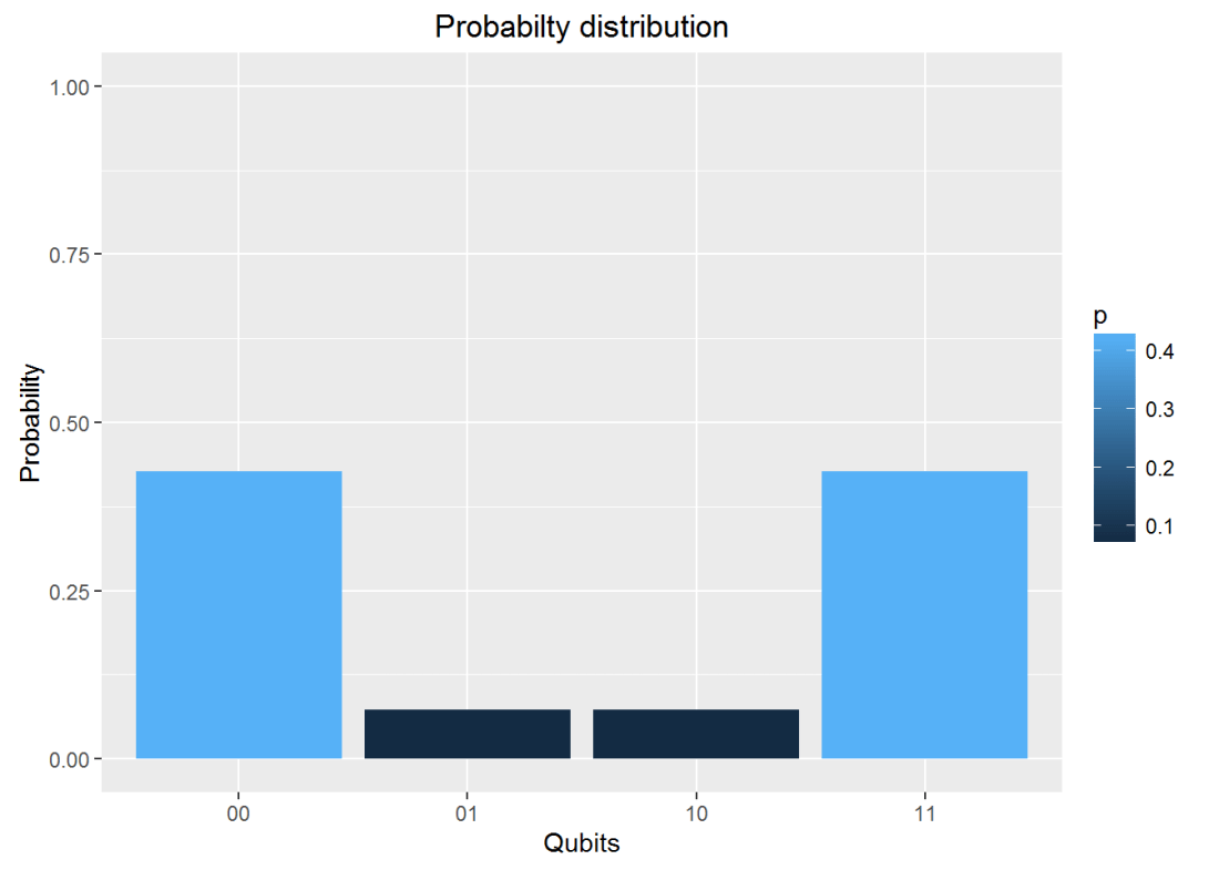
a = TensorProd(PauliZ(I2),Hadamard(I2))
b = DotProduct(a,q00_)
plotMeasurement(measurement(b))

8. Measurement

The measurement of a Quantum circuit can be obtained using the measurement function. Consider the following Quantum circuit
Q0 – H-T-H-T-S-H-T-H-T-H-T-H-S-Measurement where H – Hadamard gate, T – T Gate and S- S Gate

a = SGate(Hadamard(TGate(Hadamard(TGate(Hadamard(TGate(Hadamard(SGate(TGate(Hadamard(TGate(Hadamard(I2)))))))))))))
measurement(a)

##          0        1
## v 0.890165 0.109835

9. Plot measurement

Using the same example as above Q0 – H-T-H-T-S-H-T-H-T-H-T-H-S-Measurement where H – Hadamard gate, T – T Gate and S- S Gate we can plot the measurement

a = SGate(Hadamard(TGate(Hadamard(TGate(Hadamard(TGate(Hadamard(SGate(TGate(Hadamard(TGate(Hadamard(I2)))))))))))))
result = measurement(a)
plotMeasurement(result)

10. Evaluating a Quantum Circuit

The above procedures for evaluating a quantum gates in series and parallel can be used to evalute more complex quantum circuits where the quantum gates are in series and in parallel.

Here is an evaluation of one such circuit, the Bell ZQ state using the QCSimulator (from IBM’s Quantum Experience)

# 1st composite
a = TensorProd(Hadamard(I2),I2)
# Output of CNOT
b = CNOT2_01(a)
# 2nd series
c=Hadamard(TGate(Hadamard(SGate(I2))))
#3rd composite
d= TensorProd(I2,c)
# Output of 2nd composite
e = DotProduct(b,d)
#Action of quantum circuit on |00>
f = DotProduct(e,q00_)
result= measurement(f)
plotMeasurement(result)

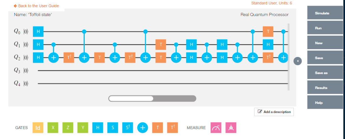
11. Toffoli State

This circuit for this comes from IBM’s Quantum Experience. This circuit is available in the package. This is how the state was constructed. This circuit is shown below

The implementation of the above circuit in QCSimulator is as below

  # Computation of the Toffoli State
    H=1/sqrt(2) * matrix(c(1,1,1,-1),nrow=2,ncol=2)
    I=matrix(c(1,0,0,1),nrow=2,ncol=2)

    # 1st composite
    # H x H x H
    a = TensorProd(TensorProd(H,H),H)
    # 1st CNOT
    a1= CNOT3_12(a)

    # 2nd composite
    # I x I x T1Gate
    b = TensorProd(TensorProd(I,I),T1Gate(I))
    b1 = DotProduct(b,a1)
    c = CNOT3_02(b1)

    # 3rd composite
    # I x I x TGate
    d = TensorProd(TensorProd(I,I),TGate(I))
    d1 = DotProduct(d,c)
    e = CNOT3_12(d1)

    # 4th composite
    # I x I x T1Gate
    f = TensorProd(TensorProd(I,I),T1Gate(I))
    f1 = DotProduct(f,e)
    g = CNOT3_02(f1)

    #5th composite
    # I x T x T
    h = TensorProd(TensorProd(I,TGate(I)),TGate(I))
    h1 = DotProduct(h,g)
    i = CNOT3_12(h1)

    #6th composite
    # I x H x H
    j = TensorProd(TensorProd(I,Hadamard(I)),Hadamard(I))
    j1 = DotProduct(j,i)
    k = CNOT3_12(j1)

    # 7th composite
    # I x H x H
    l = TensorProd(TensorProd(I,Hadamard(I)),Hadamard(I))
    l1 = DotProduct(l,k)
    m = CNOT3_12(l1)
    n = CNOT3_02(m)

    #8th composite
    # T x H x T1
    o = TensorProd(TensorProd(TGate(I),Hadamard(I)),T1Gate(I))
    o1 = DotProduct(o,n)
    p = CNOT3_02(o1)
    result = measurement(p)
    plotMeasurement(result)

12. GHZ YYX measurement

Here is another Quantum circuit, namely the entangled GHZ YYX state. This is

and is implemented in QCSimulator as

# Composite 1
a = TensorProd(TensorProd(Hadamard(I2),Hadamard(I2)),PauliX(I2))
b= CNOT3_12(a)
c= CNOT3_02(b)
# Composite 2
d= TensorProd(TensorProd(Hadamard(I2),Hadamard(I2)),Hadamard(I2))
e= DotProduct(d,c)
#Composite 3
f= TensorProd(TensorProd(S1Gate(I2),S1Gate(I2)),Hadamard(I2))
g= DotProduct(f,e)
#Composite 4
i= TensorProd(TensorProd(Hadamard(I2),Hadamard(I2)),I2)
j = DotProduct(i,g)
result=measurement(j)
plotMeasurement(result)

Conclusion

The 5 qubit Quantum Computing Simulator is now fully functional. I hope to add more gates and functionality in the months to come.

Feel free to install the package from Github and give it a try.

Disclaimer: This article represents the author’s viewpoint only and doesn’t necessarily represent IBM’s positions, strategies or opinions

References

My other posts on Quantum Computing

You may also like
For more posts on other topics like Cloud Computing, IBM Bluemix, Distributed Computing, OpenCV, R, cricket please check my Index of posts

Taking a closer look at Quantum gates and their operations

This post is a continuation of my earlier post ‘Exploring Quantum gate operations with QCSimulator’. Here I take a closer look at more quantum gates and their operations, besides implementing these new gates in my Quantum Computing simulator, the QCSimulator in R.

Disclaimer: This article represents the author’s viewpoint only and doesn’t necessarily represent IBM’s positions, strategies or opinions

In quantum circuits, gates are unitary matrices which operate on 1,2 or 3 qubit systems which are represented as below

1 qubit
|0> = $\begin{pmatrix}1\\0\end{pmatrix}$ and |1> = $\begin{pmatrix}0\\1\end{pmatrix}$

2 qubits
|0> $\otimes$ |0> = $\begin{pmatrix}1\\ 0\\ 0\\0\end{pmatrix}$
|0> $\otimes$ |1> = $\begin{pmatrix}0\\ 1\\ 0\\0\end{pmatrix}$
|1> $\otimes$ |o> = $\begin{pmatrix}0\\ 0\\ 1\\0\end{pmatrix}$
|1> $\otimes$ |1> = $\begin{pmatrix}0\\ 0\\ 0\\1\end{pmatrix}$

3 qubits
|0> $\otimes$ |0> $\otimes$ |0> = $\begin{pmatrix}1\\ 0\\0\\ 0\\ 0\\0\\ 0\\0\end{pmatrix}$
|0> $\otimes$ |0> $\otimes$ |1> = $\begin{pmatrix}0\\ 1\\0\\ 0\\ 0\\0\\ 0\\0\end{pmatrix}$
|0> $\otimes$ |1> $\otimes$ |0> = $\begin{pmatrix}0\\ 0\\1\\ 0\\ 0\\0\\ 0\\0\end{pmatrix}$
…
…
|1> $\otimes$ |1> $\otimes$ |1> = $\begin{pmatrix}0\\ 0\\0\\ 0\\ 0\\0\\ 0\\1\end{pmatrix}$
Hence single qubit is represented as 2 x 1 matrix, 2 qubit as 4 x 1 matrix and 3 qubit as 8 x 1 matrix

1) Composing Quantum gates in series
When quantum gates are connected in a series. The overall effect of the these quantum gates in series is obtained my taking the dot product of the unitary gates in reverse. For e.g.

In the following picture the effect of the quantum gates A,B,C is the dot product of the gates taken reverse order
result = C . B . A

This overall action of the 3 quantum gates can be represented by a single ‘transfer’ matrix which is the dot product of the gates

If we had a Pauli X followed by a Hadamard gate the combined effect of these gates on the inputs can be deduced by constructing a truth table

Input	Pauli X – Output A’	Hadamard – Output B
\|0>	\|1>	1/√2(\|0> – \|1>)
\|1>	\|0>	1/√2(\|0> + \|1>)

|0> -> 1/√2(|0> – |1>)
|1> -> 1/√2(|0> + |1>)
which is
$\begin{pmatrix}1\\0\end{pmatrix}$ ->1/√2 $\begin{pmatrix}1\\0\end{pmatrix}$ – $\begin{pmatrix}0\\1\end{pmatrix}$ = 1/√2 $\begin{pmatrix}1\\-1\end{pmatrix}$
$\begin{pmatrix}0\\1\end{pmatrix}$ ->1/√2 $\begin{pmatrix}1\\0\end{pmatrix}$ + $\begin{pmatrix}0\\1\end{pmatrix}$ = 1/√2 $\begin{pmatrix}1\\1\end{pmatrix}$
Therefore the ‘transfer’ matrix can be written as
T = 1/√2 $\begin{pmatrix}1 & 1\\ -1 & 1\end{pmatrix}$

2)Quantum gates in parallel
When quantum gates are in parallel then the composite effect of the gates can be obtained by taking the tensor product of the quantum gates.

If we consider the combined action of a Pauli X gate and a Hadamard gate in parallel

A	B	A’	B’
\|0>	\|0>	\|1>	1/√2(\|0> + \|1>)
\|0>	\|1>	\|1>	1/√2(\|0> – \|1>)
\|1>	\|0>	\|0>	1/√2(\|0> + \|1>)
\|1>	\|1>	\|0>	1/√2(\|0> – \|1>)

|00> => |1> $\otimes$ 1/√2(|0> + |1>) = 1/√2 (|10> + |11>)
|01> => |1> $\otimes$ 1/√2(|0> – |1>) = 1/√2 (|10> – |11>)
|10> => |0> $\otimes$ 1/√2(|0> + |1>) = 1/√2 (|00> + |01>)
|11> => |0> $\otimes$ 1/√2(|0> – |1>) = 1/√2 (|10> – |11>)

|00> = $\begin{pmatrix}1\\ 0\\ 0\\0\end{pmatrix}$ =>1/√2 $\begin{pmatrix} 0\\ 0\\ 1\\ 1\end{pmatrix}$
|01> = $\begin{pmatrix}0\\ 1\\ 0\\0\end{pmatrix}$ =>1/√2 $\begin{pmatrix} 0\\ 0\\ 1\\ -1\end{pmatrix}$
|10> = $\begin{pmatrix}0\\ 0\\ 1\\0\end{pmatrix}$ =>1/√2 $\begin{pmatrix} 1\\ 0\\ 1\\ -1\end{pmatrix}$
|11> = $\begin{pmatrix}0\\ 0\\ 0\\1\end{pmatrix}$ =>1/√2 $\begin{pmatrix} 1\\ 0\\ -1\\ -1\end{pmatrix}$

Here are more Quantum gates
a) Rotation gate
$U = \begin{pmatrix}cos\theta & -sin\theta\\ sin\theta & cos\theta\end{pmatrix}$

b) Toffoli gate
The Toffoli gate flips the 3^rd qubit if the 1^st and 2^nd qubit are |1>

Toffoli gate
Input	Output
\|000>	\|000>
\|001>	\|001>
\|010>	\|010>
\|011>	\|011>
\|100>	\|100>
\|101>	\|101>
\|110>	\|111>
\|111>	\|110>

c) Fredkin gate
The Fredkin gate swaps the 2^nd and 3^rd qubits if the 1^st qubit is |1>

Fredkin gate
Input	Output
\|000>	\|000>
\|001>	\|001>
\|010>	\|010>
\|011>	\|011>
\|100>	\|100>
\|101>	\|110>
\|110>	\|101>
\|111>	\|111>

d) Controlled U gate
A controlled U gate can be represented as
controlled U = $\begin{pmatrix}1 & 0 & 0 & 0\\ 0 &1 &0 & 0\\ 0 &0 &u11 &u12 \\ 0 & 0 &u21 &u22 \end{pmatrix}$ – (A)
where U = $\begin{pmatrix}u11 &u12 \\ u21 & u22\end{pmatrix}$

e) Controlled Pauli gates
Controlled Pauli gates are created based on the following identities. The CNOT gate is a controlled Pauli X gate where controlled U is a Pauli X gate and matches the CNOT unitary matrix. Pauli gates can be constructed using

a) H x X x H = Z &
H x H = I

b) S x X x S1
S x S1 = I

the controlled Pauli X, Y , Z are contructed using the CNOT for the controlled X in the above identities
In general a controlled Pauli gate can be created as below

f) CPauliX
Here C is the 2 x2 Identity matrix. Simulating this in my QCSimulator
CPauliX I=matrix(c(1,0,0,1),nrow=2,ncol=2) # Compute 1st composite a = TensorProd(I,I) b = CNOT2_01(a) # Compute 1st composite c = TensorProd(I,I) #Take dot product d = DotProduct(c,b) #Take dot product with qubit e = DotProduct(d,q) e }

Implementing the above with I, S, H gives Pauli X, Y and Z as seen below

library(QCSimulator)
I4=matrix(c(1,0,0,0,
            0,1,0,0,
            0,0,1,0,
            0,0,0,1),nrow=4,ncol=4)

#Controlled Pauli X
CPauliX(I4)

##      [,1] [,2] [,3] [,4]
## [1,]    1    0    0    0
## [2,]    0    1    0    0
## [3,]    0    0    0    1
## [4,]    0    0    1    0

#Controlled Pauli Y
CPauliY(I4)

##      [,1] [,2] [,3] [,4]
## [1,] 1+0i 0+0i 0+0i 0+0i
## [2,] 0+0i 1+0i 0+0i 0+0i
## [3,] 0+0i 0+0i 0+0i 0-1i
## [4,] 0+0i 0+0i 0+1i 0+0i

#Controlled Pauli Z
CPauliZ(I4)

##      [,1] [,2] [,3] [,4]
## [1,]    1    0    0    0
## [2,]    0    1    0    0
## [3,]    0    0    1    0
## [4,]    0    0    0   -1

g) CSWAP gate

q00=matrix(c(1,0,0,0),nrow=4,ncol=1)
q01=matrix(c(0,1,0,0),nrow=4,ncol=1)
q10=matrix(c(0,0,1,0),nrow=4,ncol=1)
q11=matrix(c(0,0,0,1),nrow=4,ncol=1)
CSWAP(q00)

##      [,1]
## [1,]    1
## [2,]    0
## [3,]    0
## [4,]    0

#Swap qubits 
CSWAP(q01)

##      [,1]
## [1,]    0
## [2,]    0
## [3,]    1
## [4,]    0

#Swap qubits 
CSWAP(q10)

##      [,1]
## [1,]    0
## [2,]    1
## [3,]    0
## [4,]    0

CSWAP(q11)

##      [,1]
## [1,]    0
## [2,]    0
## [3,]    0
## [4,]    1

h) Toffoli state
The Toffoli state creates a 3 qubit entangled state 1/2(|000> + |001> + |100> + |111>)

Simulating the Toffoli state in IBM Quantum Experience we get

h) Implementation of Toffoli state in QCSimulator

#ToffoliState 
    # Computation of the Toffoli State
    H=1/sqrt(2) * matrix(c(1,1,1,-1),nrow=2,ncol=2)
    I=matrix(c(1,0,0,1),nrow=2,ncol=2)

    # 1st composite
    # H x H x H
    a = TensorProd(TensorProd(H,H),H)
    # 1st CNOT
    a1= CNOT3_12(a)

    # 2nd composite
    # I x I x T1Gate
    b = TensorProd(TensorProd(I,I),T1Gate(I))
    b1 = DotProduct(b,a1)
    c = CNOT3_02(b1)

    # 3rd composite
    # I x I x TGate
    d = TensorProd(TensorProd(I,I),TGate(I))
    d1 = DotProduct(d,c)
    e = CNOT3_12(d1)

    # 4th composite
    # I x I x T1Gate
    f = TensorProd(TensorProd(I,I),T1Gate(I))
    f1 = DotProduct(f,e)
    g = CNOT3_02(f1)

    #5th composite
    # I x T x T
    h = TensorProd(TensorProd(I,TGate(I)),TGate(I))
    h1 = DotProduct(h,g)
    i = CNOT3_12(h1)

    #6th composite
    # I x H x H
    j = TensorProd(TensorProd(I,Hadamard(I)),Hadamard(I))
    j1 = DotProduct(j,i)
    k = CNOT3_12(j1)

    # 7th composite
    # I x H x H
    l = TensorProd(TensorProd(I,Hadamard(I)),Hadamard(I))
    l1 = DotProduct(l,k)
    m = CNOT3_12(l1)
    n = CNOT3_02(m)

    #8th composite
    # T x H x T1
    o = TensorProd(TensorProd(TGate(I),Hadamard(I)),T1Gate(I))
    o1 = DotProduct(o,n)
    p = CNOT3_02(o1)
    result = measurement(p)
    plotMeasurement(result)

The measurement is identical to the that of IBM Quantum Experience

Conclusion: This post looked at more Quantum gates. I have implemented all the gates in my QCSimulator which I hope to release in a couple of months.

Disclaimer: This article represents the author’s viewpoint only and doesn’t necessarily represent IBM’s positions, strategies or opinions

References
1. http://www1.gantep.edu.tr/~koc/qc/chapter4.pdf
2. http://iontrap.umd.edu/wp-content/uploads/2016/01/Quantum-Gates-c2.pdf
3. https://quantumexperience.ng.bluemix.net/

Also see
1. Venturing into IBM’s Quantum Experience
2. Going deeper into IBM’s Quantum Experience!
3. A primer on Qubits, Quantum gates and Quantum Operations
4. Exploring Quantum gate operations with QCSimulator

Take a look at my other posts at
1. Index of posts

Exploring Quantum Gate operations with QCSimulator

Introduction: Ever since I was initiated into Quantum Computing, through IBM’s Quantum Experience I have been hooked. My initial encounter with domain made me very excited and all wound up. The reason behind this, I think, is because there is an air of mystery around ‘Quantum’ anything. After my early rush with the Quantum Experience, I have deliberately slowed down to digest the heady stuff.

This post also includes my early prototype of a Quantum Computing Simulator( QCSimulator) which I am creating in R. I hope to have a decent Quantum Computing simulator available, in the next couple of months. The ideas for this simulator are based on IBM’s Quantum Experience and the lectures on Quantum Mechanics and Quantum Computation by Prof Umesh Vazirani from University of California at Berkeley at edX. This calls to this simulator have been included in R Markdown file and has been published at RPubs as Quantum Computing Simulator

Disclaimer: This article represents the author’s viewpoint only and doesn’t necessarily represent IBM’s positions, strategies or opinions

In this post I explore quantum gate operations

A) Quantum Gates
Quantum gates are represented as a n x n unitary matrix. In mathematics, a complex square matrix U is unitary if its conjugate transpose U^ǂ is also its inverse – that is, if
U^ǂU =U U^ǂ=I

a) Clifford Gates
The following gates are known as Clifford Gates and are represented as the unitary matrix below

1. Pauli X
$\begin{pmatrix}0&1\\1&0\end{pmatrix}$

2.Pauli Y
$\begin{pmatrix}0&-i\\i&0\end{pmatrix}$

3. Pauli Z
$\begin{pmatrix}1&0\\0&-1\end{pmatrix}$

4. Hadamard
1/√2 $\begin{pmatrix}1 & 1\\ 1 & -1\end{pmatrix}$

5. S Gate
$\begin{pmatrix}1 & 0\\ 0 & i\end{pmatrix}$

6. S1 Gate
$\begin{pmatrix}1 & 0\\ 0 & -i\end{pmatrix}$

7. CNOT
$\begin{pmatrix}1 & 0 & 0 &0 \\ 0 & 1 & 0 &0 \\ 0& 0 & 0&1 \\ 0 & 0 & 1 & 0\end{pmatrix}$

b) Non-Clifford Gate
The following are the non-Clifford gates
1. Toffoli Gate
T = $\begin{pmatrix}1 & 0\\ 0 & e^{^{i\prod /4}}\end{pmatrix}$

2. Toffoli1 Gate
T1 = $\begin{pmatrix}1 & 0\\ 0 & e^{^{-i\prod /4}}\end{pmatrix}$

B) Evolution of a 1 qubit Quantum System
The diagram below shows how a 1 qubit system evolves on the application of Quantum Gates.

C) Evolution of a 2 Qubit System
The following diagram depicts the evolution of a 2 qubit system. The 4 different maximally entangled states can be obtained by using a Hadamard and a CNOT gate to |00>, |01>, |10> & |11> resulting in the entangled states Φ⁺, Ψ⁺, Φ^–, Ψ^–respectively

D) Verifying Unitary’ness
XX^ǂ = X^ǂX= I
TT^ǂ = T^ǂT=I
SS^ǂ = S^ǂS=I
The U^ǂ function in the simulator is
U^ǂ = GateDagger(U)

E) A look at some Simulator functions
The unitary functions for the Clifford and non-Clifford gates have been implemented functions. The unitary functions can be chained together by invoking each successive Gate as argument to the function.

1. Creating the dagger function
HDagger = GateDagger(Hadamard)
HDagger x Hadamard
TDagger = GateDagger(TGate)
TDagger x TGate

##           [,1]       [,2]
## [1,] 0.7071068  0.7071068
## [2,] 0.7071068 -0.7071068

HDagger = GateDagger(H)
HDagger

##           [,1]       [,2]
## [1,] 0.7071068  0.7071068
## [2,] 0.7071068 -0.7071068

HDagger %*% H

##      [,1] [,2]
## [1,]    1    0
## [2,]    0    1

##      [,1]                 [,2]
## [1,] 1+0i 0.0000000+0.0000000i
## [2,] 0+0i 0.7071068+0.7071068i

TDagger = GateDagger(T)
TDagger

##      [,1]                 [,2]
## [1,] 1+0i 0.0000000+0.0000000i
## [2,] 0+0i 0.7071068-0.7071068i

TDagger %*% T

##      [,1] [,2]
## [1,] 1+0i 0+0i
## [2,] 0+0i 1+0i

2. Angle between 2 vectors – Inner product
The angle between 2 vectors can be obtained by taking the inner product between the vectors

#1. a is the diagonal vector 1/2 |0> + 1/2 |1> and b = q0 = |0>
diagonal <-  matrix(c(1/sqrt(2),1/sqrt(2)),nrow=2,ncol=1)
q0=matrix(c(1,0),nrow=2,ncol=1)
innerProduct(diagonal,q0)

##      [,1]
## [1,]   45

#2. a = 1/2|0> + sqrt(3)/2|1> and  b= 1/sqrt(2) |0> + 1/sqrt(2) |1>
a = matrix(c(1/2,sqrt(3)/2),nrow=2,ncol=1)
b = matrix(c(1/sqrt(2),1/sqrt(2)),nrow=2,ncol=1)
innerProduct(a,b)

##      [,1]
## [1,]   15

3. Chaining Quantum Gates
For e.g.
H x q0
S x H x q0 == > SGate(Hadamard(q0))

Or
H x S x S x H x q0 == > Hadamard(SGate(SGate(Hadamard))))

# H x q0
Hadamard(q0)

##           [,1]
## [1,] 0.7071068
## [2,] 0.7071068

# S x H x q0
SGate(Hadamard(q0))

##                      [,1]
## [1,] 0.7071068+0.0000000i
## [2,] 0.0000000+0.7071068i

# H x S x S x H x q0
Hadamard(SGate(SGate(Hadamard(q0))))

##      [,1]
## [1,] 0+0i
## [2,] 1+0i

# S x T x H x T x H x q0
SGate(TGate(Hadamard(TGate(Hadamard(q0)))))

##                      [,1]
## [1,] 0.8535534+0.3535534i
## [2,] 0.1464466+0.3535534i

4. Measurement
The output of Quantum Gate operations can be measured with
measurement(a)
measurement(q0)
measurement(Hadamard(q0))
a=SGate(TGate(Hadamard(TGate(Hadamard(I)))))
measurement(a)
measurement(SGate(TGate(Hadamard(TGate(Hadamard(I))))))

measurement(q0)

##   0 1
## v 1 0

measurement(Hadamard(q0))

##     0   1
## v 0.5 0.5

a <- SGate(TGate(Hadamard(TGate(Hadamard(q0)))))
measurement(a)

##           0         1
## v 0.8535534 0.1464466

5. Plot the measurements

plotMeasurement(q1)

plotMeasurement(Hadamard(q0))

a = measurement(SGate(TGate(Hadamard(TGate(Hadamard(q0))))))
plotMeasurement(a)

6. Using the QCSimulator for one of the Bell tests
Here I compute the following measurement of Bell state ZW with the QCSimulator

When this is simulated on IBM’s Quantum Experience the result is

Below I simulate the same on my R based QCSimulator

# Compute the effect of the Composite H gate with the Identity matrix (I)
a=kronecker(H,I,"*")
a

##           [,1]      [,2]       [,3]       [,4]
## [1,] 0.7071068 0.0000000  0.7071068  0.0000000
## [2,] 0.0000000 0.7071068  0.0000000  0.7071068
## [3,] 0.7071068 0.0000000 -0.7071068  0.0000000
## [4,] 0.0000000 0.7071068  0.0000000 -0.7071068

# Compute the applcation of CNOT on this result
b = CNOT(a)
b

##           [,1]      [,2]       [,3]       [,4]
## [1,] 0.7071068 0.0000000  0.7071068  0.0000000
## [2,] 0.0000000 0.7071068  0.0000000  0.7071068
## [3,] 0.0000000 0.7071068  0.0000000 -0.7071068
## [4,] 0.7071068 0.0000000 -0.7071068  0.0000000

# Obtain the result of CNOT on q00
c = b %*% q00
c

##           [,1]
## [1,] 0.7071068
## [2,] 0.0000000
## [3,] 0.0000000
## [4,] 0.7071068

# Compute the effect of the composite HxTxHxS gates and the Identity matrix(I) for measurement
d=Hadamard(TGate(Hadamard(SGate(I))))
e=kronecker(I, d,"*")

# Applying  the composite gate on the output 'c'
f = e %*% c
# Measure the output
g <- measurement(f)
g

##          00        01        10        11
## v 0.4267767 0.0732233 0.0732233 0.4267767

#Plot the measurement
plotMeasurement(g)

aa
which is exactly the result obtained with IBM’s Quantum Experience!

Conclusion : In this post I dwell on 1 and 2-qubit quantum gates and explore their operation. I have started to construct a R based Quantum Computing Simulator. I hope to have a reasonable simulator in the next couple of months. Let’s see.

Watch this space!

Disclaimer: This article represents the author’s viewpoint only and doesn’t necessarily represent IBM’s positions, strategies or opinions

References
1. IBM Quantum Experience – User Guide
2. Quantum Mechanics and Quantum Conputing, UC Berkeley

Also see
1. Venturing into IBM’s Quantum Experience
2. Going deeper into IBM’s Quantum Experience!
3. A primer on Qubits, Quantum gates and Quantum Operations

For more posts see
Index of posts

Re-introducing cricketr! : An R package to analyze performances of cricketers

In this post I re-introduce R package cricketr. I have added 8 new functions to my R package cricketr, available from version cricketr_0.0.13 namely

batsmanCumulativeAverageRuns
batsmanCumulativeStrikeRate
bowlerCumulativeAvgEconRate
bowlerCumulativeAvgWicketRate
relativeBatsmanCumulativeAvgRuns
relativeBatsmanCumulativeStrikeRate
relativeBowlerCumulativeAvgWickets
relativeBowlerCumulativeAvgEconRate

This post updates my earlier post Introducing cricketr:An R package for analyzing performances of cricketrs

Yet all experience is an arch wherethro’
Gleams that untravell’d world whose margin fades
For ever and forever when I move.
How dull it is to pause, to make an end,
To rust unburnish’d, not to shine in use!
Ulysses by Alfred Tennyson

Introduction

This is an initial post in which I introduce a cricketing package ‘cricketr’ which I have created. This package was a natural culmination to my earlier posts on cricket and my finishing 10 modules of Data Science Specialization, from John Hopkins University at Coursera. The thought of creating this package struck me some time back, and I have finally been able to bring this to fruition.

So here it is. My R package ‘cricketr!!!’

If you are passionate about cricket, and love analyzing cricket performances, then check out my racy book on cricket ‘Cricket analytics with cricketr and cricpy – Analytics harmony with R & Python’! This book discusses and shows how to use my R package ‘cricketr’ and my Python package ‘cricpy’ to analyze batsmen and bowlers in all formats of the game (Test, ODI and T20). The paperback is available on Amazon at $21.99 and the kindle version at $9.99/Rs 449/-. A must read for any cricket lover! Check it out!!

You can download the latest PDF version of the book at ‘Cricket analytics with cricketr and cricpy: Analytics harmony with R and Python-6th edition‘

Untitled

This package uses the statistics info available in ESPN Cricinfo Statsguru. The current version of this package can handle all formats of the game including Test, ODI and Twenty20 cricket.

You should be able to install the package from GitHub and use many of the functions available in the package. Please be mindful of ESPN Cricinfo Terms of Use

Important note 1: The latest release of ‘cricketr’ now includes the ability to analyze performances of teams now!! See Cricketr adds team analytics to its repertoire!!!

Important note 2 : Cricketr can now do a more fine-grained analysis of players, see Cricketr learns new tricks : Performs fine-grained analysis of players

Important note 3: Do check out the python avatar of cricketr, ‘cricpy’ in my post ‘Introducing cricpy:A python package to analyze performances of cricketers”

Note: This page is also hosted as a GitHub page at cricketr

This post is also hosted on Rpubs at Reintroducing cricketr. You can also down the pdf version of this post at reintroducing_cricketr.pdf

(Take a look at my short video tutorial on my R package cricketr on Youtube – R package cricketr – A short tutorial)

Do check out my interactive Shiny app implementation using the cricketr package – Sixer – R package cricketr’s new Shiny avatar

Also see my 2nd book “Beaten by sheer pace” based on my R package yorkr which is now available in paperback and kindle versions at Amazon

Note: If you would like to do a similar analysis for a different set of batsman and bowlers, you can clone/download my skeleton cricketr template from Github (which is the R Markdown file I have used for the analysis below). You will only need to make appropriate changes for the players you are interested in. Just a familiarity with R and R Markdown only is needed.

The cricketr package

The cricketr package has several functions that perform several different analyses on both batsman and bowlers. The package has functions that plot percentage frequency runs or wickets, runs likelihood for a batsman, relative run/strike rates of batsman and relative performance/economy rate for bowlers are available.

Other interesting functions include batting performance moving average, forecast and a function to check whether the batsman/bowler is in in-form or out-of-form.

The data for a particular player can be obtained with the getPlayerData() function from the package. To do this you will need to go to ESPN CricInfo Player and type in the name of the player for e.g Ricky Ponting, Sachin Tendulkar etc. This will bring up a page which have the profile number for the player e.g. for Sachin Tendulkar this would be http://www.espncricinfo.com/india/content/player/35320.html. Hence, Sachin’s profile is 35320. This can be used to get the data for Tendulkar as shown below

The cricketr package is now available from CRAN!!!. You should be able to install directly with

# Install from CRAN
if (!require("cricketr")){ 
    install.packages("cricketr",lib = "c:/test") 
} 
library(cricketr)

Getting help from cricketr

?getPlayerData

## 
## getPlayerData(profile, opposition='', host='', dir='./data', file='player001.csv', type='batting', homeOrAway=[1, 2], result=[1, 2, 4], create=True)
##     Get the player data from ESPN Cricinfo based on specific inputs and store in a file in a given directory
##     
##     Description
##     
##     Get the player data given the profile of the batsman. The allowed inputs are home,away or both and won,lost or draw of matches. The data is stored in a .csv file in a directory specified. This function also returns a data frame of the player
##     
##     Usage
##     
##     getPlayerData(profile,opposition="",host="",dir="./data",file="player001.csv",
##     type="batting", homeOrAway=c(1,2),result=c(1,2,4))
##     Arguments
##     
##     profile     
##     This is the profile number of the player to get data. This can be obtained from http://www.espncricinfo.com/ci/content/player/index.html. Type the name of the player and click search. This will display the details of the player. Make a note of the profile ID. For e.g For Sachin Tendulkar this turns out to be http://www.espncricinfo.com/india/content/player/35320.html. Hence the profile for Sachin is 35320
##     opposition  
##     The numerical value of the opposition country e.g.Australia,India, England etc. The values are Australia:2,Bangladesh:25,England:1,India:6,New Zealand:5,Pakistan:7,South Africa:3,Sri Lanka:8, West Indies:4, Zimbabwe:9
##     host        
##     The numerical value of the host country e.g.Australia,India, England etc. The values are Australia:2,Bangladesh:25,England:1,India:6,New Zealand:5,Pakistan:7,South Africa:3,Sri Lanka:8, West Indies:4, Zimbabwe:9
##     dir 
##     Name of the directory to store the player data into. If not specified the data is stored in a default directory "./data". Default="./data"
##     file        
##     Name of the file to store the data into for e.g. tendulkar.csv. This can be used for subsequent functions. Default="player001.csv"
##     type        
##     type of data required. This can be "batting" or "bowling"
##     homeOrAway  
##     This is a vector with either 1,2 or both. 1 is for home 2 is for away
##     result      
##     This is a vector that can take values 1,2,4. 1 - won match 2- lost match 4- draw
##     Details
##     
##     More details can be found in my short video tutorial in Youtube https://www.youtube.com/watch?v=q9uMPFVsXsI
##     
##     Value
##     
##     Returns the player's dataframe
##     
##     Note
##     
##     Maintainer: Tinniam V Ganesh <tvganesh.85@gmail.com>
##     
##     Author(s)
##     
##     Tinniam V Ganesh
##     
##     References
##     
##     http://www.espncricinfo.com/ci/content/stats/index.html
##     https://gigadom.wordpress.com/
##     
##     See Also
##     
##     getPlayerDataSp
##     
##     Examples
##     
##     ## Not run: 
##     # Both home and away. Result = won,lost and drawn
##     tendulkar = getPlayerData(35320,dir=".", file="tendulkar1.csv",
##     type="batting", homeOrAway=c(1,2),result=c(1,2,4))
##     
##     # Only away. Get data only for won and lost innings
##     tendulkar = getPlayerData(35320,dir=".", file="tendulkar2.csv",
##     type="batting",homeOrAway=c(2),result=c(1,2))
##     
##     # Get bowling data and store in file for future
##     kumble = getPlayerData(30176,dir=".",file="kumble1.csv",
##     type="bowling",homeOrAway=c(1),result=c(1,2))
##     
##     #Get the Tendulkar's Performance against Australia in Australia
##     tendulkar = getPlayerData(35320, opposition = 2,host=2,dir=".", 
##     file="tendulkarVsAusInAus.csv",type="batting")

The cricketr package includes some pre-packaged sample (.csv) files. You can use these sample to test functions as shown below

# Retrieve the file path of a data file installed with cricketr
pathToFile ,"Sachin Tendulkar")

Alternatively, the cricketr package can be installed from GitHub with

if (!require("cricketr")){ 
    library(devtools) 
    install_github("tvganesh/cricketr") 
}
library(cricketr)

The pre-packaged files can be accessed as shown above.
To get the data of any player use the function getPlayerData()

tendulkar <- getPlayerData(35320,dir="..",file="tendulkar.csv",type="batting",homeOrAway=c(1,2),
                           result=c(1,2,4))

Important Note This needs to be done only once for a player. This function stores the player’s data in a CSV file (for e.g. tendulkar.csv as above) which can then be reused for all other functions. Once we have the data for the players many analyses can be done. This post will use the stored CSV file obtained with a prior getPlayerData for all subsequent analyses

Sachin Tendulkar’s performance – Basic Analyses

The 3 plots below provide the following for Tendulkar

Frequency percentage of runs in each run range over the whole career
Mean Strike Rate for runs scored in the given range
A histogram of runs frequency percentages in runs ranges

par(mfrow=c(1,3))
par(mar=c(4,4,2,2))
batsmanRunsFreqPerf("./tendulkar.csv","Sachin Tendulkar")
batsmanMeanStrikeRate("./tendulkar.csv","Sachin Tendulkar")
batsmanRunsRanges("./tendulkar.csv","Sachin Tendulkar")

dev.off()

## null device 
##           1

More analyses

par(mfrow=c(1,3))
par(mar=c(4,4,2,2))
batsman4s("./tendulkar.csv","Tendulkar")
batsman6s("./tendulkar.csv","Tendulkar")
batsmanDismissals("./tendulkar.csv","Tendulkar")

3D scatter plot and prediction plane

The plots below show the 3D scatter plot of Sachin’s Runs versus Balls Faced and Minutes at crease. A linear regression model is then fitted between Runs and Balls Faced + Minutes at crease

battingPerf3d("./tendulkar.csv","Sachin Tendulkar")

Average runs at different venues

The plot below gives the average runs scored by Tendulkar at different grounds. The plot also displays the number of innings at each ground as a label at x-axis. It can be seen Tendulkar did great in Colombo (SSC), Melbourne ifor matches overseas and Mumbai, Mohali and Bangalore at home

batsmanAvgRunsGround("./tendulkar.csv","Sachin Tendulkar")

Average runs against different opposing teams

This plot computes the average runs scored by Tendulkar against different countries. The x-axis also gives the number of innings against each team

batsmanAvgRunsOpposition("./tendulkar.csv","Tendulkar")

Highest Runs Likelihood

The plot below shows the Runs Likelihood for a batsman. For this the performance of Sachin is plotted as a 3D scatter plot with Runs versus Balls Faced + Minutes at crease using. K-Means. The centroids of 3 clusters are computed and plotted. In this plot. Sachin Tendulkar’s highest tendencies are computed and plotted using K-Means

batsmanRunsLikelihood("./tendulkar.csv","Sachin Tendulkar")

## Summary of  Sachin Tendulkar 's runs scoring likelihood
## **************************************************
## 
## There is a 16.51 % likelihood that Sachin Tendulkar  will make  139 Runs in  251 balls over 353  Minutes 
## There is a 58.41 % likelihood that Sachin Tendulkar  will make  16 Runs in  31 balls over  44  Minutes 
## There is a 25.08 % likelihood that Sachin Tendulkar  will make  66 Runs in  122 balls over 167  Minutes

A look at the Top 4 batsman – Tendulkar, Kallis, Ponting and Sangakkara

The batsmen with the most hundreds in test cricket are

Sachin Tendulkar :Average:53.78,100’s – 51, 50’s – 68
Jacques Kallis : Average: 55.47, 100’s – 45, 50’s – 58
Ricky Ponting : Average: 51.85, 100’s – 41 , 50’s – 62
Kumara Sangakarra: Average: 58.04 ,100’s – 38 , 50’s – 52

in that order.

The following plots take a closer at their performances. The box plots show the mean (red line) and median (blue line). The two ends of the boxplot display the 25th and 75th percentile.

Box Histogram Plot

This plot shows a combined boxplot of the Runs ranges and a histogram of the Runs Frequency. The calculated Mean differ from the stated means possibly because of data cleaning. Also not sure how the means were arrived at ESPN Cricinfo for e.g. when considering not out..

batsmanPerfBoxHist("./tendulkar.csv","Sachin Tendulkar")

batsmanPerfBoxHist("./kallis.csv","Jacques Kallis")

batsmanPerfBoxHist("./ponting.csv","Ricky Ponting")

batsmanPerfBoxHist("./sangakkara.csv","K Sangakkara")

Contribution to won and lost matches

The plot below shows the contribution of Tendulkar, Kallis, Ponting and Sangakarra in matches won and lost. The plots show the range of runs scored as a boxplot (25th & 75th percentile) and the mean scored. The total matches won and lost are also printed in the plot.

All the players have scored more in the matches they won than the matches they lost. Ricky Ponting is the only batsman who seems to have more matches won to his credit than others. This could also be because he was a member of strong Australian team

For the next 2 functions below you will have to use the getPlayerDataSp() function. I
have commented this as I already have these files

tendulkarsp

par(mfrow=c(2,2))
par(mar=c(4,4,2,2))
batsmanContributionWonLost("tendulkarsp.csv","Tendulkar")
batsmanContributionWonLost("kallissp.csv","Kallis")
batsmanContributionWonLost("pontingsp.csv","Ponting")
batsmanContributionWonLost("sangakkarasp.csv","Sangakarra")

dev.off()

## null device 
##           1

Performance at home and overseas

From the plot below it can be seen
Tendulkar has more matches overseas than at home and his performance is consistent in all venues at home or abroad. Ponting has lesser innings than Tendulkar and has an equally good performance at home and overseas.Kallis and Sangakkara’s performance abroad is lower than the performance at home.

This function also requires the use of getPlayerDataSp() as shown above

par(mfrow=c(2,2))
par(mar=c(4,4,2,2))
batsmanPerfHomeAway("tendulkarsp.csv","Tendulkar")
batsmanPerfHomeAway("kallissp.csv","Kallis")
batsmanPerfHomeAway("pontingsp.csv","Ponting")
batsmanPerfHomeAway("sangakkarasp.csv","Sangakarra")
dev.off()

dev.off()

## null device 
##           1

Moving Average of runs in career

Take a look at the Moving Average across the career of the Top 4. Clearly . Kallis and Sangakkara have a few more years of great batting ahead. They seem to average on 50. . Tendulkar and Ponting definitely show a slump in the later years

par(mfrow=c(2,2))
par(mar=c(4,4,2,2))
batsmanMovingAverage("./tendulkar.csv","Sachin Tendulkar")
batsmanMovingAverage("./kallis.csv","Jacques Kallis")
batsmanMovingAverage("./ponting.csv","Ricky Ponting")
batsmanMovingAverage("./sangakkara.csv","K Sangakkara")

dev.off()

## null device 
##           1

Cumulative Average runs of batsman in career

This function provides the cumulative average runs of the batsman over the career. Tendulkar averages around 50, while Sangakkarra touches 55 towards the end of his career

par(mfrow=c(2,2))
par(mar=c(4,4,2,2))
batsmanCumulativeAverageRuns("./tendulkar.csv","Tendulkar")

batsmanCumulativeAverageRuns("./kallis.csv","Kallis")

batsmanCumulativeAverageRuns("./ponting.csv","Ponting")

batsmanCumulativeAverageRuns("./sangakkara.csv","Sangakkara")

dev.off()

## null device 
##           1

Cumulative Average strike rate of batsman in career

This function gives the cumulative strike rate of the batsman over the career

par(mfrow=c(2,2))
par(mar=c(4,4,2,2))
batsmanCumulativeStrikeRate("./tendulkar.csv","Tendulkar")

batsmanCumulativeStrikeRate("./kallis.csv","Kallis")

batsmanCumulativeStrikeRate("./ponting.csv","Ponting")

batsmanCumulativeStrikeRate("./sangakkara.csv","Sangakkara")

dev.off()

## null device 
##           1

Future Runs forecast

Here are plots that forecast how the batsman will perform in future. In this case 90% of the career runs trend is uses as the training set. the remaining 10% is the test set.

A Holt-Winters forecating model is used to forecast future performance based on the 90% training set. The forecated runs trend is plotted. The test set is also plotted to see how close the forecast and the actual matches

Take a look at the runs forecasted for the batsman below.

Tendulkar’s forecasted performance seems to tally with his actual performance with an average of 50
Kallis the forecasted runs are higher than the actual runs he scored
Ponting seems to have a good run in the future
Sangakkara has a decent run in the future averaging 50 runs

par(mfrow=c(2,2))
par(mar=c(4,4,2,2))
batsmanPerfForecast("./tendulkar.csv","Sachin Tendulkar")
batsmanPerfForecast("./kallis.csv","Jacques Kallis")
batsmanPerfForecast("./ponting.csv","Ricky Ponting")
batsmanPerfForecast("./sangakkara.csv","K Sangakkara")

dev.off()

## null device 
##           1

Relative Mean Strike Rate plot

The plot below compares the Mean Strike Rate of the batsman for each of the runs ranges of 10 and plots them. The plot indicate the following Range 0 – 50 Runs – Ponting leads followed by Tendulkar Range 50 -100 Runs – Ponting followed by Sangakkara Range 100 – 150 – Ponting and then Tendulkar

frames <- list("./tendulkar.csv","./kallis.csv","ponting.csv","sangakkara.csv")
names <- list("Tendulkar","Kallis","Ponting","Sangakkara")
relativeBatsmanSR(frames,names)

Relative Runs Frequency plot

The plot below gives the relative Runs Frequency Percetages for each 10 run bucket. The plot below show

Sangakkara leads followed by Ponting

frames <- list("./tendulkar.csv","./kallis.csv","ponting.csv","sangakkara.csv")
names <- list("Tendulkar","Kallis","Ponting","Sangakkara")
relativeRunsFreqPerf(frames,names)

Relative cumulative average runs in career

The plot below compares the relative cumulative runs of the batsmen over the career. While Tendulkar seems to lead over the others with a cumulative average of 50, we can see that Sangakkara goes over everybody else between 180-220th inning. It is likely that Sangakkarra may have overtaken Tendulkar if he had played more

frames <- list("./tendulkar.csv","./kallis.csv","ponting.csv","sangakkara.csv")
names <- list("Tendulkar","Kallis","Ponting","Sangakkara")
relativeBatsmanCumulativeAvgRuns(frames,names)

Relative cumulative average strike rate in career

As seen in earlier charts Ponting has the best overall strike rate, followed by Sangakkara and then Tendulkar

frames <- list("./tendulkar.csv","./kallis.csv","ponting.csv","sangakkara.csv")
names <- list("Tendulkar","Kallis","Ponting","Sangakkara")
relativeBatsmanCumulativeStrikeRate(frames,names)

Check Batsman In-Form or Out-of-Form

The below computation uses Null Hypothesis testing and p-value to determine if the batsman is in-form or out-of-form. For this 90% of the career runs is chosen as the population and the mean computed. The last 10% is chosen to be the sample set and the sample Mean and the sample Standard Deviation are caculated.

The Null Hypothesis (H0) assumes that the batsman continues to stay in-form where the sample mean is within 95% confidence interval of population mean The Alternative (Ha) assumes that the batsman is out of form the sample mean is beyond the 95% confidence interval of the population mean.

A significance value of 0.05 is chosen and p-value us computed If p-value >= .05 – Batsman In-Form If p-value < 0.05 – Batsman Out-of-Form

Note Ideally the p-value should be done for a population that follows the Normal Distribution. But the runs population is usually left skewed. So some correction may be needed. I will revisit this later

This is done for the Top 4 batsman

checkBatsmanInForm("./tendulkar.csv","Sachin Tendulkar")

## *******************************************************************************************
## 
## Population size: 294  Mean of population: 50.48 
## Sample size: 33  Mean of sample: 32.42 SD of sample: 29.8 
## 
## Null hypothesis H0 : Sachin Tendulkar 's sample average is within 95% confidence interval 
##         of population average
## Alternative hypothesis Ha : Sachin Tendulkar 's sample average is below the 95% confidence
##         interval of population average
## 
## [1] "Sachin Tendulkar 's Form Status: Out-of-Form because the p value: 0.000713  is less than alpha=  0.05"
## *******************************************************************************************

checkBatsmanInForm("./kallis.csv","Jacques Kallis")

## *******************************************************************************************
## 
## Population size: 240  Mean of population: 47.5 
## Sample size: 27  Mean of sample: 47.11 SD of sample: 59.19 
## 
## Null hypothesis H0 : Jacques Kallis 's sample average is within 95% confidence interval 
##         of population average
## Alternative hypothesis Ha : Jacques Kallis 's sample average is below the 95% confidence
##         interval of population average
## 
## [1] "Jacques Kallis 's Form Status: In-Form because the p value: 0.48647  is greater than alpha=  0.05"
## *******************************************************************************************

checkBatsmanInForm("./ponting.csv","Ricky Ponting")

## *******************************************************************************************
## 
## Population size: 251  Mean of population: 47.5 
## Sample size: 28  Mean of sample: 36.25 SD of sample: 48.11 
## 
## Null hypothesis H0 : Ricky Ponting 's sample average is within 95% confidence interval 
##         of population average
## Alternative hypothesis Ha : Ricky Ponting 's sample average is below the 95% confidence
##         interval of population average
## 
## [1] "Ricky Ponting 's Form Status: In-Form because the p value: 0.113115  is greater than alpha=  0.05"
## *******************************************************************************************

checkBatsmanInForm("./sangakkara.csv","K Sangakkara")

## *******************************************************************************************
## 
## Population size: 193  Mean of population: 51.92 
## Sample size: 22  Mean of sample: 71.73 SD of sample: 82.87 
## 
## Null hypothesis H0 : K Sangakkara 's sample average is within 95% confidence interval 
##         of population average
## Alternative hypothesis Ha : K Sangakkara 's sample average is below the 95% confidence
##         interval of population average
## 
## [1] "K Sangakkara 's Form Status: In-Form because the p value: 0.862862  is greater than alpha=  0.05"
## *******************************************************************************************

3D plot of Runs vs Balls Faced and Minutes at Crease

The plot is a scatter plot of Runs vs Balls faced and Minutes at Crease. A prediction plane is fitted

par(mfrow=c(1,2))
par(mar=c(4,4,2,2))
battingPerf3d("./tendulkar.csv","Tendulkar")
battingPerf3d("./kallis.csv","Kallis")
par(mfrow=c(1,2))
par(mar=c(4,4,2,2))
battingPerf3d("./ponting.csv","Ponting")
battingPerf3d("./sangakkara.csv","Sangakkara")
dev.off()

## null device 
##           1

Predicting Runs given Balls Faced and Minutes at Crease

A multi-variate regression plane is fitted between Runs and Balls faced +Minutes at crease. A sample sequence of Balls Faced(BF) and Minutes at crease (Mins) is setup as shown below. The fitted model is used to predict the runs for these values

BF <- seq( 10, 400,length=15)
Mins <- seq(30,600,length=15)
newDF <- data.frame(BF,Mins)
tendulkar <- batsmanRunsPredict("./tendulkar.csv","Tendulkar",newdataframe=newDF)
kallis <- batsmanRunsPredict("./kallis.csv","Kallis",newdataframe=newDF)
ponting <- batsmanRunsPredict("./ponting.csv","Ponting",newdataframe=newDF)
sangakkara <- batsmanRunsPredict("./sangakkara.csv","Sangakkara",newdataframe=newDF)

The fitted model is then used to predict the runs that the batsmen will score for a given Balls faced and Minutes at crease. It can be seen Ponting has the will score the highest for a given Balls Faced and Minutes at crease.

Ponting is followed by Tendulkar who has Sangakkara close on his heels and finally we have Kallis. This is intuitive as we have already seen that Ponting has a highest strike rate.

batsmen <-cbind(round(tendulkar$Runs),round(kallis$Runs),round(ponting$Runs),round(sangakkara$Runs))
colnames(batsmen) <- c("Tendulkar","Kallis","Ponting","Sangakkara")
newDF <- data.frame(round(newDF$BF),round(newDF$Mins))
colnames(newDF) <- c("BallsFaced","MinsAtCrease")
predictedRuns <- cbind(newDF,batsmen)
predictedRuns

##    BallsFaced MinsAtCrease Tendulkar Kallis Ponting Sangakkara
## 1          10           30         7      6       9          2
## 2          38           71        23     20      25         18
## 3          66          111        39     34      42         34
## 4          94          152        54     48      59         50
## 5         121          193        70     62      76         66
## 6         149          234        86     76      93         82
## 7         177          274       102     90     110         98
## 8         205          315       118    104     127        114
## 9         233          356       134    118     144        130
## 10        261          396       150    132     161        146
## 11        289          437       165    146     178        162
## 12        316          478       181    159     194        178
## 13        344          519       197    173     211        194
## 14        372          559       213    187     228        210
## 15        400          600       229    201     245        226

Checkout my book ‘Deep Learning from first principles Second Edition- In vectorized Python, R and Octave’. My book is available on Amazon as paperback ($18.99) and in kindle version($9.99/Rs449).

You may also like my companion book “Practical Machine Learning with R and Python:Second Edition- Machine Learning in stereo” available in Amazon in paperback($12.99) and Kindle($9.99/Rs449) versions.

Analysis of Top 3 wicket takers

The top 3 wicket takes in test history are
1. M Muralitharan:Wickets: 800, Average = 22.72, Economy Rate – 2.47
2. Shane Warne: Wickets: 708, Average = 25.41, Economy Rate – 2.65
3. Anil Kumble: Wickets: 619, Average = 29.65, Economy Rate – 2.69

How do Anil Kumble, Shane Warne and M Muralitharan compare with one another with respect to wickets taken and the Economy Rate. The next set of plots compute and plot precisely these analyses.

Wicket Frequency Plot

This plot below computes the percentage frequency of number of wickets taken for e.g 1 wicket x%, 2 wickets y% etc and plots them as a continuous line

par(mfrow=c(1,3))
par(mar=c(4,4,2,2))
bowlerWktsFreqPercent("./kumble.csv","Anil Kumble")
bowlerWktsFreqPercent("./warne.csv","Shane Warne")
bowlerWktsFreqPercent("./murali.csv","M Muralitharan")

dev.off()

## null device 
##           1

Wickets Runs plot

par(mfrow=c(1,3))
par(mar=c(4,4,2,2))
bowlerWktsRunsPlot("./kumble.csv","Kumble")
bowlerWktsRunsPlot("./warne.csv","Warne")
bowlerWktsRunsPlot("./murali.csv","Muralitharan")

dev.off()

## null device 
##           1

Average wickets at different venues

The plot gives the average wickets taken by Muralitharan at different venues. Muralitharan has taken an average of 8 and 6 wickets at Oval & Wellington respectively in 2 different innings. His best performances are at Kandy and Colombo (SSC)

bowlerAvgWktsGround("./murali.csv","Muralitharan")

Average wickets against different opposition

The plot gives the average wickets taken by Muralitharan against different countries. The x-axis also includes the number of innings against each team

bowlerAvgWktsOpposition("./murali.csv","Muralitharan")

Wickets taken moving average

From th eplot below it can be see 1. Shane Warne’s performance at the time of his retirement was still at a peak of 3 wickets 2. M Muralitharan seems to have become ineffective over time with his peak years being 2004-2006 3. Anil Kumble also seems to slump down and become less effective.

par(mfrow=c(1,3))
par(mar=c(4,4,2,2))
bowlerMovingAverage("./kumble.csv","Anil Kumble")
bowlerMovingAverage("./warne.csv","Shane Warne")
bowlerMovingAverage("./murali.csv","M Muralitharan")

dev.off()

## null device 
##           1

Cumulative average wickets taken

The plots below give the cumulative average wickets taken by the bowlers

par(mfrow=c(1,3))
par(mar=c(4,4,2,2))
bowlerCumulativeAvgWickets("./kumble.csv","Kumble")

bowlerCumulativeAvgWickets("./warne.csv","Warne")

bowlerCumulativeAvgWickets("./murali.csv","Muralitharan")

dev.off()

## null device 
##           1

Cumulative average economy rate

The plots below give the cumulative average economy rate of the bowlers

par(mfrow=c(1,3))
par(mar=c(4,4,2,2))
bowlerCumulativeAvgEconRate("./kumble.csv","Kumble")

bowlerCumulativeAvgEconRate("./warne.csv","Warne")

bowlerCumulativeAvgEconRate("./murali.csv","Muralitharan")

dev.off()

## null device 
##           1

Future Wickets forecast

Here are plots that forecast how the bowler will perform in future. In this case 90% of the career wickets trend is used as the training set. the remaining 10% is the test set.

A Holt-Winters forecating model is used to forecast future performance based on the 90% training set. The forecated wickets trend is plotted. The test set is also plotted to see how close the forecast and the actual matches

Take a look at the wickets forecasted for the bowlers below. – Shane Warne and Muralitharan have a fairly consistent forecast – Kumble forecast shows a small dip

par(mfrow=c(1,3))
par(mar=c(4,4,2,2))
bowlerPerfForecast("./kumble.csv","Anil Kumble")
bowlerPerfForecast("./warne.csv","Shane Warne")
bowlerPerfForecast("./murali.csv","M Muralitharan")

dev.off()

## null device 
##           1

Contribution to matches won and lost

The plot below is extremely interesting
1. Kumble wickets range from 2 to 4 wickets in matches wons with a mean of 3
2. Warne wickets in won matches range from 1 to 4 with more matches won. Clearly there are other bowlers contributing to the wins, possibly the pacers
3. Muralitharan wickets range in winning matches is more than the other 2 and ranges ranges 3 to 5 and clearly had a hand (pun unintended) in Sri Lanka’s wins

As discussed above the next 2 charts require the use of getPlayerDataSp()

kumblesp

par(mfrow=c(1,3))
par(mar=c(4,4,2,2))
bowlerContributionWonLost("kumblesp.csv","Kumble")
bowlerContributionWonLost("warnesp.csv","Warne")
bowlerContributionWonLost("muralisp.csv","Murali")

dev.off()

## null device 
##           1

Performance home and overseas

From the plot below it can be seen that Kumble & Warne have played more matches overseas than Muralitharan. Both Kumble and Warne show an average of 2 wickers overseas, Murali on the other hand has an average of 2.5 wickets overseas but a slightly less number of matches than Kumble & Warne

par(mfrow=c(1,3))
par(mar=c(4,4,2,2))
bowlerPerfHomeAway("kumblesp.csv","Kumble")
bowlerPerfHomeAway("warnesp.csv","Warne")
bowlerPerfHomeAway("muralisp.csv","Murali")

dev.off()

## null device 
##           1

Relative Wickets Frequency Percentage

The Relative Wickets Percentage plot shows that M Muralitharan has a large percentage of wickets in the 3-8 wicket range

frames <- list("./kumble.csv","./murali.csv","warne.csv")
names <- list("Anil KUmble","M Muralitharan","Shane Warne")
relativeBowlingPerf(frames,names)

Relative Economy Rate against wickets taken

Clearly from the plot below it can be seen that Muralitharan has the best Economy Rate among the three

frames <- list("./kumble.csv","./murali.csv","warne.csv")
names <- list("Anil KUmble","M Muralitharan","Shane Warne")
relativeBowlingER(frames,names)

Relative cumulative average wickets of bowlers in career

The plot below shows that Murali has the best cumulative average wickets taken followed by Kumble and then Warne

frames <- list("./kumble.csv","./murali.csv","warne.csv")
names <- list("Anil KUmble","M Muralitharan","Shane Warne")
relativeBowlerCumulativeAvgWickets(frames,names)

Relative cumulative average economy rate of bowlers

Muralitharan has the best economy rate followed by Warne and then Kumble

frames <- list("./kumble.csv","./murali.csv","warne.csv")
names <- list("Anil KUmble","M Muralitharan","Shane Warne")
relativeBowlerCumulativeAvgEconRate(frames,names)

Check for bowler in-form/out-of-form

The below computation uses Null Hypothesis testing and p-value to determine if the bowler is in-form or out-of-form. For this 90% of the career wickets is chosen as the population and the mean computed. The last 10% is chosen to be the sample set and the sample Mean and the sample Standard Deviation are caculated.

The Null Hypothesis (H0) assumes that the bowler continues to stay in-form where the sample mean is within 95% confidence interval of population mean The Alternative (Ha) assumes that the bowler is out of form the sample mean is beyond the 95% confidence interval of the population mean.

A significance value of 0.05 is chosen and p-value us computed If p-value >= .05 – Batsman In-Form If p-value < 0.05 – Batsman Out-of-Form

Note: The check for the form status of the bowlers indicate 1. That both Kumble and Muralitharan were out of form. This also shows in the moving average plot 2. Warne is still in great form and could have continued for a few more years. Too bad we didn’t see the magic later

checkBowlerInForm("./kumble.csv","Anil Kumble")

## *******************************************************************************************
## 
## Population size: 212  Mean of population: 2.69 
## Sample size: 24  Mean of sample: 2.04 SD of sample: 1.55 
## 
## Null hypothesis H0 : Anil Kumble 's sample average is within 95% confidence interval 
##         of population average
## Alternative hypothesis Ha : Anil Kumble 's sample average is below the 95% confidence
##         interval of population average
## 
## [1] "Anil Kumble 's Form Status: Out-of-Form because the p value: 0.02549  is less than alpha=  0.05"
## *******************************************************************************************

checkBowlerInForm("./warne.csv","Shane Warne")

## *******************************************************************************************
## 
## Population size: 240  Mean of population: 2.55 
## Sample size: 27  Mean of sample: 2.56 SD of sample: 1.8 
## 
## Null hypothesis H0 : Shane Warne 's sample average is within 95% confidence interval 
##         of population average
## Alternative hypothesis Ha : Shane Warne 's sample average is below the 95% confidence
##         interval of population average
## 
## [1] "Shane Warne 's Form Status: In-Form because the p value: 0.511409  is greater than alpha=  0.05"
## *******************************************************************************************

checkBowlerInForm("./murali.csv","M Muralitharan")

## *******************************************************************************************
## 
## Population size: 207  Mean of population: 3.55 
## Sample size: 23  Mean of sample: 2.87 SD of sample: 1.74 
## 
## Null hypothesis H0 : M Muralitharan 's sample average is within 95% confidence interval 
##         of population average
## Alternative hypothesis Ha : M Muralitharan 's sample average is below the 95% confidence
##         interval of population average
## 
## [1] "M Muralitharan 's Form Status: Out-of-Form because the p value: 0.036828  is less than alpha=  0.05"
## *******************************************************************************************

dev.off()

## null device 
##           1

Key Findings

The plots above capture some of the capabilities and features of my cricketr package. Feel free to install the package and try it out. Please do keep in mind ESPN Cricinfo’s Terms of Use.
Here are the main findings from the analysis above

Analysis of Top 4 batsman

The analysis of the Top 4 test batsman Tendulkar, Kallis, Ponting and Sangakkara show the folliwing

Sangakkara has the highest average, followed by Tendulkar, Kallis and then Ponting.
Ponting has the highest strike rate followed by Tendulkar,Sangakkara and then Kallis
The predicted runs for a given Balls faced and Minutes at crease is highest for Ponting, followed by Tendulkar, Sangakkara and Kallis
The moving average for Tendulkar and Ponting shows a downward trend while Kallis and Sangakkara retired too soon
Tendulkar was out of form about the time of retirement while the rest were in-form. But this result has to be taken along with the moving average plot. Ponting was clearly on the way out.
The home and overseas performance indicate that Tendulkar is the clear leader. He has the highest number of matches played overseas and his performance has been consistent. He is followed by Ponting, Kallis and finally Sangakkara

Analysis of Top 3 legs spinners

The analysis of Anil Kumble, Shane Warne and M Muralitharan show the following

Muralitharan has the highest wickets and best economy rate followed by Warne and Kumble
Muralitharan has higher wickets frequency percentage between 3 to 8 wickets
Muralitharan has the best Economy Rate for wickets between 2 to 7
The moving average plot shows that the time was up for Kumble and Muralitharan but Warne had a few years ahead
The check for form status shows that Muralitharan and Kumble time was over while Warne still in great form
Kumble’s has more matches abroad than the other 2, yet Kumble averages of 3 wickets at home and 2 wickets overseas liek Warne . Murali has played few matches but has an average of 4 wickets at home and 3 wickets overseas.

Final thoughts

Here are my final thoughts

Batting

Among the 4 batsman Tendulkar, Kallis, Ponting and Sangakkara the clear leader is Tendulkar for the following reasons

Tendulkar has the highest test centuries and runs of all time.Tendulkar’s average is 2nd to Sangakkara, Tendulkar’s predicted runs for a given Balls faced and Minutes at Crease is 2nd and is behind Ponting. Also Tendulkar’s performance at home and overseas are consistent throughtout despite the fact that he has a highest number of overseas matches
Ponting takes the 2nd spot with the 2nd highest number of centuries, 1st in Strike Rate and 2nd in home and away performance.
The 3rd spot goes to Sangakkara, with the highest average, 3rd highest number of centuries, reasonable run frequency percentage in different run ranges. However he has a fewer number of matches overseas and his performance overseas is significantly lower than at home
Kallis has the 2nd highest number of centuries but his performance overseas and strike rate are behind others
Finally Kallis and Sangakkara had a few good years of batting still left in them (pity they retired!) while Tendulkar and Ponting’s time was up
While Tendulkars cumulative average stays around 50 runs, Sangakkara briefly overtakes Tendulkar towards the end of his career. Sangakkara may have finished with a better average if he had played for a few more years
Ponting has the best overall strike rate followed by Sangakkara

Bowling

Muralitharan leads the way followed closely by Warne and finally Kumble. The reasons are

Muralitharan has the highest number of test wickets with the best Wickets percentage and the best Economy Rate. Murali on average gas taken 4 wickets at home and 3 wickets overseas
Warne follows Murali in the highest wickets taken, however Warne has less matches overseas than Murali and average 3 wickets home and 2 wickets overseas
Kumble has the 3rd highest wickets, with 3 wickets on an average at home and 2 wickets overseas. However Kumble has played more matches overseas than the other two. In that respect his performance is great. Also Kumble has played less matches at home otherwise his numbers would have looked even better.
Also while Kumble and Muralitharan’s career was on the decline , Warne was going great and had a couple of years ahead.
Muralitharan has the best cumulative wicket rate and economy rate. Kumble has a better wicket rate than Warne but is more expensive than Warne

You can download this analysis at Introducing cricketrYou can download this analysis at Re-Introducing cricketr

Important note: Do check out my other posts using cricketr at cricketr-posts

Also see

1.Introducing cricket package yorkr-Part1:Beaten by sheer pace!.
2.yorkr pads up for the Twenty20s: Part 1- Analyzing team“s match performance.
3.yorkr crashes the IPL party !Part 1
4.Introducing cricketr! : An R package to analyze performances of cricketers
5.Beaten by sheer pace! Cricket analytics with yorkr in paperback and Kindle versions
6. Cricket analytics with cricketr in paperback and Kindle versions

Beaten by sheer pace! Cricket analytics with yorkr in paperback and Kindle versions

My book “Beaten by sheer pace! Cricket analytics with yorkr” is now available in paperback and Kindle versions. The paperback is available from Amazon (US, UK and Europe) for $ 54.95. The Kindle version can be downloaded from the Kindle store for $4.99 (Rs 332/-). Do pick up your copy. It should be a good read for a Sunday afternoon.

This book of mine contains my posts based on my R package ‘yorkr’ now in CRAN. The package yorkr uses the data from Cricsheet (http://cricsheet.org/) and can perform analysis of ODI and T20 matches. yorkr can analyze teams against a specific opposition or all oppositions, besides providing details on batsmen or bowlers individual performances The analyses include team batting partnerships, performances of batsmen against bowlers, bowlers against batsmen, bowlers best performances etc. Individual analyses of batsmen strike rate, cumulative average, bowler economy rate, bowler moving average etc can be performances

The book includes the following chapters based on my R package yorkr.

CONTENTS
Preface
Foreword
1.Introducing cricket package yorkr: Part 1- Beaten by sheer pace!
2.Introducing cricket package yorkr: Part 2-Trapped leg before wicket!
3.Introducing cricket package yorkr: Part 3-Foxed by flight!
4.Introducing cricket package yorkr:Part 4-In the block hole!
5.yorkr pads up for the Twenty20s: Part 1- Analyzing team’s match performance!
6.yorkr pads up for the Twenty20s: Part 2-Head to head confrontation between teams
7.yorkr pads up for the Twenty20s:Part 3:Overall team performance against all oppositions!
8.yorkr pads up for Twenty20s:Part 4- Individual batting and bowling performances!
9.yorkr crashes the IPL party ! – Part 1
10.yorkr crashes the IPL party! – Part 2
11.yorkr crashes the IPL party! – Part 3!
12.yorkr crashes the IPL party! – Part 4
13.yorkr ranks IPL batsmen and bowlers
14.yorkr ranks T20 batsmen and bowlers
15.yorkr ranks ODI batsmen and bowlers
16.yorkr is generic!
Important links
Afterword
Other books by author
About the author

Checkout my interactive Shiny apps GooglyPlus (plots & tables) and Googly (only plots) which can be used to analyze IPL players, teams and matches.

Beaten by sheer pace – Cricket analytics with yorkr

My ebook “Beaten by sheer pace – Cricket analytics with yorkr’ has been published in Leanpub. You can now download the book (hot off the press!) for all formats to your favorite device (mobile, iPad, tablet, Kindle) from the Leanpub “Beaten by sheer pace!”. The book has been published in the following formats namely

PDF (for your computer)
EPUB (for iPad or tablets. Save the file cricketAnalyticsWithYorkr.epub to Google Drive/Dropbox and choose “Open in” iBooks for iPad)
MOBI (for Kindle. For this format, I suggest that you download & install SendToKindle for PC/Mac. You can then right click the downloaded cricketAnalyticsWithYorkr.mobi and choose SendToKindle. You will need to login to your Kindle account)

From Leanpub
Leanpub uses a variable pricing model. I have priced the book attractively (I think!). You can choose a price between FREE (limited time offer!) to $4.99 . The link is “Beaten by sheer pace!”

This format works with all type Kindle device, Kindle app, Android tablet, iPad.

Checkout my interactive Shiny apps GooglyPlus (plots & tables) and Googly (only plots) which can be used to analyze IPL players, teams and matches.

yorkr is generic!

The features and functionality in my yorkr package is now complete. My R package yorkr, is totally generic, which means that the R package can be used for all ODI, T20 matches. Hence yorkr can be used for professional or amateur ODI and T20 matches. The R package can be used for both men and women ODI, T20 international or domestic matches. The main requirement is, that the match data be created as a Yaml file in the format Cricsheet (Required yaml format for the match data).

If you are passionate about cricket, and love analyzing cricket performances, then check out my 2 racy books on cricket! In my books, I perform detailed yet compact analysis of performances of both batsmen, bowlers besides evaluating team & match performances in Tests , ODIs, T20s & IPL. You can buy my books on cricket from Amazon at $12.99 for the paperback and $4.99/$6.99 respectively for the kindle versions. The books can be accessed at Cricket analytics with cricketr and Beaten by sheer pace-Cricket analytics with yorkr A must read for any cricket lover! Check it out!!

$4.99/Rs 320 and $6.99/Rs448 respectively

I have successfully used my R functions for the Indian Premier League (IPL) matches with changes only to the convertAllYamlFiles2RDataFramesXX (please see posts below)

The convertAllYamlFiles2RDataframes &convertAllYamlFiles2RDataFramesT20 will have to be customized for the names of the teams playing in the domestic professional or amateur matches. All other classes of functions namely Class1, Class2, Class 3 and Class 4 as discussed in my post Introducing cricket package yorkr-Part 1: Beaten by sheer pace can be used as is without any changes.

There are numerous professional & amateur T20 matches that are played around the world. Here are a list of domestic T20 tournaments that are played around the world (from Wikipedia). The yorkr package can be used for any of these matches once the match data is saved as yaml as mentioned above.

So do go ahead and have fun, analyzing cricket performances with yorkr!

Please take a look at my posts on how to use yorkr for ODI, Twenty20 matches.

Introducing cricket package yorkr:Part 1- Beaten by sheer pace!
2. Introducing cricket package yorkr:Part 2- Trapped leg before wicket!
3. Introducing cricket package yorkr:Part 3- foxed by flight!
4. Introducing cricket package yorkr:Part 4-In the block hole!
5. yorkr pads up for the Twenty20s: Part 1- Analyzing team”s match performance
6. yorkr pads up for the Twenty20s: Part 2-Head to head confrontation between teams
7. yorkr pads up for the Twenty20s:Part 3:Overall team performance against all oppositions!
8. yorkr pads up for Twenty20s:Part 4- Individual batting and bowling performances!
9. yorkr crashes the IPL party ! – Part 1
10. yorkr crashes the IPL party! – Part 2
11. yorkr crashes the IPL party! – Part 3
12. yorkr crashes the IPL party! – Part 4
13. yorkr ranks IPL batsmen and bowlers
14. yorkr ranks T20 batsmen and bowlers
15. yorkr ranks ODI batsmen and bowlers

yorkr ranks ODI batsmen and bowlers

This is the last and final post in which yorkr ranks ODI batsmen and bowlers. These are based on match data from Cricsheet. The ranking is done on

average runs and average strike rate for batsmen and
average wickets and average economy rate for bowlers.

nd $4.99/Rs 320 and $6.99/Rs448 respectively

This post has also been published in RPubs RankODIPlayers. You can download this as a pdf file at RankODIPlayers.pdf.

Checkout my interactive Shiny apps GooglyPlus (plots & tables) and Googly (only plots) which can be used to analyze IPL players, teams and matches.

You can take a look at the code at rankODIPlayers (available in yorkr_0.0.5)

rm(list=ls())
library(yorkr)
library(dplyr)
source("rankODIBatsmen.R")
source("rankODIBowlers.R")

Rank ODI batsmen

The top 3 ODI batsmen are hashim Amla (SA), Matther Hayden(Aus) & Virat Kohli (Ind) . Note: For ODI a a cutoff of at least 50 matches played was chosen.

ODIBatsmanRank <- rankODIBatsmen()
as.data.frame(ODIBatsmanRank[1:30,])

##            batsman matches meanRuns    meanSR
## 1          HM Amla     185 51.96216  84.15508
## 2        ML Hayden      79 50.08861  81.20646
## 3          V Kohli     279 48.51971  78.55197
## 4   AB de Villiers     253 47.93676  95.05561
## 5     SR Tendulkar     151 45.82119  79.62311
## 6         S Dhawan     116 45.03448  81.54043
## 7         V Sehwag     167 44.49102 106.27563
## 8          JE Root     111 43.64865  81.66054
## 9        Q de Kock      85 43.61176  82.55235
## 10       IJL Trott     113 43.36283  70.69761
## 11   KC Sangakkara     293 42.81911  75.10420
## 12      TM Dilshan     283 41.76678  89.70360
## 13   KS Williamson     146 41.24658  73.49267
## 14   S Chanderpaul      93 40.07527  70.59613
## 15        HH Gibbs      75 40.00000  79.03813
## 16     Salman Butt      57 39.85965  59.29807
## 17    Anamul Haque      58 39.72414  56.45224
## 18      RT Ponting     238 38.88235  71.94294
## 19       JH Kallis     136 38.77941  67.17794
## 20        MS Dhoni     328 38.57927  90.30555
## 21      MJ Guptill     199 38.54774  73.88090
## 22       DA Warner     138 38.52174  87.24978
## 23 Mohammad Yousuf      94 38.44681  72.69851
## 24        JD Ryder      66 38.40909  91.29667
## 25       GJ Bailey     133 38.38346  75.74519
## 26       G Gambhir     209 37.83254  75.15483
## 27      AJ Strauss     122 37.80328  71.54844
## 28       MJ Clarke     301 37.67442  69.78415
## 29       SR Watson     274 37.08029  83.46489
## 30        AJ Finch     103 36.36893  79.49845

Rank ODI bowlers

The top 3 ODI bowlers are R J Harris (Aus), MJ Henry(NZ) and MA Starc(Aus). Mohammed Shami is 4th and Amit Mishra is 8th A cutoff of 20 matches was considered for bowlers

ODIBowlersRank <- rankODIBowlers()

## [1] 35072     3
## [1] "C:/software/cricket-package/york-test/yorkrData/ODI/ODI-matches"

as.data.frame(ODIBowlersRank[1:30,])

##               bowler matches meanWickets   meanER
## 1  Mustafizur Rahman      56    4.000000 4.293214
## 2           JH Davey      53    3.528302 4.455094
## 3          RJ Harris      94    3.276596 4.361489
## 4           MA Starc     208    3.144231 4.425865
## 5           MJ Henry      88    3.125000 4.961250
## 6         A Flintoff     139    2.956835 4.283022
## 7           A Mishra     106    2.886792 4.365849
## 8     Mohammed Shami     144    2.777778 5.609306
## 9     MJ McClenaghan     165    2.751515 5.640424
## 10          CJ McKay     230    2.704348       NA
## 11       MF Maharoof     114    2.701754 4.427018
## 12       Imran Tahir     156    2.660256 4.461923
## 13        BAW Mendis     234    2.641026 4.532308
## 14     RK Kleinveldt      54    2.629630 4.306667
## 15      Arafat Sunny      62    2.612903 4.103226
## 16         JE Taylor     156    2.602564 5.115192
## 17           AJ Hall      55    2.600000 3.879091
## 18        WD Parnell     129    2.596899 5.477597
## 19         CR Woakes     129    2.596899 5.340620
## 20      DE Bollinger     152    2.592105 4.282763
## 21        Wahab Riaz     206    2.567961 5.431748
## 22        PJ Cummins     148    2.567568 5.715405
## 23         R Rampaul     173    2.549133 4.726590
## 24      Taskin Ahmed      56    2.535714 5.325357
## 25          DW Steyn     292    2.534247 4.534007
## 26      JR Hazlewood      64    2.531250 4.392500
## 27        Abdur Rauf      84    2.523810 4.786667
## 28           SW Tait     141    2.517730 5.173191
## 29      Hamid Hassan     106    2.509434 4.686038
## 30        SL Malinga     419    2.498807 4.968974

Hope you have fun with my yorkr package.!

Important note: Do check out my other posts using yorkr at yorkr-posts

yorkr ranks T20 batsmen and bowlers

Here is another short post which ranks T20 batsmen and bowlers. These are based on match data from Cricsheet. The ranking is done on

average runs and average strike rate for batsmen and
average wickets and average economy rate for bowlers.

.99/Rs 320 and $6.99/Rs448 respectively

This post has also been published in RPubs RankT20Players. You can download this as a pdf file at RankT20Players.pdf.

Checkout my interactive Shiny apps GooglyPlus (plots & tables) and Googly (only plots) which can be used to analyze IPL players, teams and matches.

You can take a look at the code at rankT20Players (available in yorkr_0.0.5)

rm(list=ls())
library(yorkr)
library(dplyr)
source("rankT20Batsmen.R")
source("rankT20Bowlers.R")

Rank T20 batsmen

Virat Kohli (Ind), Chris Gayle (WI) and Kevin Pietersen (Eng) top the T20 rankings. Virat Kohli stands tall among the batsmen with a average of 39.1935, followed by Chris Gayle who has an average of 32.69 and finally Kevin Pietersen.

Note: For T20 a cutoff of at least 30 matches played was chosen.

T20BatsmanRank <- rankT20Batsmen()
as.data.frame(T20BatsmanRank[1:30,])

##             batsman matches meanRuns   meanSR
## 1           V Kohli      31 39.19355 128.8371
## 2          CH Gayle      43 32.69767 119.6467
## 3      KP Pietersen      37 32.43243 138.6732
## 4     KS Williamson      31 32.25806 130.1255
## 5  Mohammad Shahzad      33 31.66667 115.4582
## 6       BB McCullum      69 30.98551 126.0610
## 7        MJ Guptill      54 30.83333 120.0669
## 8          AD Hales      37 30.75676 115.3511
## 9       H Masakadza      38 29.26316 109.6182
## 10         GC Smith      32 27.59375 114.1831
## 11        DA Warner      56 27.53571 123.2209
## 12        JP Duminy      58 26.84483 117.3952
## 13 DPMD Jayawardene      51 26.47059 112.4257
## 14        SR Watson      50 26.30000 118.9464
## 15    KC Sangakkara      52 26.23077 112.4665
## 16       TM Dilshan      66 26.18182 102.5683
## 17         SK Raina      43 25.90698 124.3044
## 18        RG Sharma      41 25.68293 123.3983
## 19        G Gambhir      36 25.66667 117.5764
## 20     Yuvraj Singh      41 25.12195 119.5846
## 21    Misbah-ul-Haq      32 25.09375 106.6762
## 22       EJG Morgan      52 24.71154 121.1462
## 23       MN Samuels      40 24.35000 105.8547
## 24       MEK Hussey      30 24.03333 129.1250
## 25    Ahmed Shehzad      41 23.82927 100.8805
## 26  Shakib Al Hasan      40 23.35000 109.3798
## 27          HM Amla      30 23.33333 111.2513
## 28         CL White      45 22.73333       NA
## 29      LMP Simmons      33 22.54545       NA
## 30       Umar Akmal      69 22.20290 108.3590

Rank T20 bowlers

The top 3 T20 bowlers are BAW Mendis (SL) Umar Gul (Pak) and Steyn(SA). R Ashwin is 13th. As with batsmen, a minimum of 30 matches played was taken into consideration.

T20BowlersRank <- rankT20Bowlers()
as.data.frame(T20BowlersRank[1:30,])

##             bowler matches meanWickets   meanER
## 1       BAW Mendis      36   1.6944444 6.581111
## 2         Umar Gul      57   1.5964912 7.306842
## 3         DW Steyn      38   1.5526316 6.407632
## 4      Saeed Ajmal      63   1.4920635 6.316190
## 5       SL Malinga      59   1.4576271 7.163898
## 6       TG Southee      37   1.4054054 8.840000
## 7       MG Johnson      30   1.4000000 7.080667
## 8         GP Swann      38   1.3947368 6.576842
## 9      JW Dernbach      33   1.3636364 8.550303
## 10        M Morkel      39   1.3333333 7.384872
## 11 Shakib Al Hasan      37   1.2972973 6.648649
## 12       SP Narine      32   1.2500000 5.757812
## 13        R Ashwin      33   1.2424242 7.247273
## 14 KMDN Kulasekara      42   1.2380952 6.938095
## 15       SCJ Broad      55   1.2363636 7.832182
## 16      WD Parnell      34   1.2058824 8.227941
## 17        KD Mills      41   1.1951220 8.077317
## 18      DL Vettori      34   1.1470588 5.708235
## 19   Shahid Afridi      85   1.1294118 6.748000
## 20       SR Watson      44   1.1136364 8.015227
## 21   Sohail Tanvir      48   1.1041667 7.354167
## 22   Sohail Tanvir      48   1.1041667 7.354167
## 23     NL McCullum      56   1.0535714 7.246964
## 24     NLTC Perera      34   1.0294118 8.916471
## 25         J Botha      39   1.0256410 6.647436
## 26        DJ Bravo      45   1.0222222 8.630000
## 27   Mohammad Nabi      32   0.9687500 7.208437
## 28       DJG Sammy      55   0.8909091 7.899818
## 29 Mohammad Hafeez      56   0.8392857 6.996964
## 30      AD Mathews      44   0.7954545 6.827727

Conclusion

As expected Virat Kohli stands head and shoulders above the rest. Hamid Hasan and Mohammed Shami figuring the top T20 bowlers was a bit of a surprise to me.

Important note: Do check out my other posts using yorkr at yorkr-posts

Watch this space!

yorkr ranks IPL batsmen and bowlers

Here is a short post which ranks IPL batsmen and bowlers. These are based on match data from Cricsheet. Ranking batsmen and bowlers in IPL is more challenging as the players can belong to different teams in different years. Hence I create a combined data frame of the batsmen and bowlers regardless of their IPL teams and calculate a) average runs and average strike rate for batsmen and c) average wickets and d) average economy rate for bowlers.

I will be doing this ranking for T20 and ODI batting and bowling performances shortly.

This post has also been published in RPubs RankIPLPlayers. You can download this as a pdf file at RankIPLPlayers.pdf.

You can take a look at the code at rankIPLPlayers (should be available in yorkr_0.0.5)

Checkout my interactive Shiny apps GooglyPlus (plots & tables) and Googly (only plots) which can be used to analyze IPL players, teams and matches.

The results are slightly surprising

rm(list=ls())
library(yorkr)
library(dplyr)
setwd("C:/software/cricket-package/cricsheet/cleanup/IPL/rank")
source("rankIPLBatsmen.R")
source("rankIPLBowlers.R")

Rank IPL batsmen

Chris Gayle, MEK Hussey and Shane Watson are top 3 IPL batsmen. Gayle towers over the others in mean runs and mean strike rate. Surprisingly Ajinkya Rahane is the top Indian T20 batsman, if we leave out Sachin Tendulkar (who tops India yet again!). The other top IPL T20 batsmen are Raina, Gambhir, Rohit Sharma in that order. Virat Kohli comes a distant 14th.

iplBatsmanRank <- rankIPLBatsmen()
as.data.frame(iplBatsmanRank[1:30,])

##             batsman matches meanRuns    meanSR
## 1          CH Gayle     128 40.00781 144.92188
## 2        MEK Hussey      64 33.57812 107.23500
## 3         SR Watson      75 31.46667 129.97733
## 4      SR Tendulkar     127 29.74803 108.86622
## 5         AM Rahane      77 29.14286 101.40065
## 6         DA Warner     134 29.10448 118.38313
## 7         JP Duminy      94 28.77660 124.61702
## 8          SK Raina     128 28.62500 122.12656
## 9         G Gambhir     210 28.13810 108.78090
## 10        RG Sharma     181 28.07182 118.57801
## 11         DR Smith      78 27.82051 119.64462
## 12      BB McCullum      98 27.81633 114.91255
## 13         S Dhawan     109 27.74312 112.21000
## 14          V Kohli     188 27.56915 113.81261
## 15   AB de Villiers     150 27.46000 136.70860
## 16         R Dravid     104 27.02885 107.78923
## 17        JH Kallis     167 26.54491  94.65641
## 18         V Sehwag     174 26.39655 140.29011
## 19       RV Uthappa     166 26.27711 120.48506
## 20       SC Ganguly      86 25.98837  96.39849
## 21     AC Gilchrist      81 25.77778 122.69074
## 22    KC Sangakkara      70 25.67143 112.97529
## 23         MS Dhoni     119 25.29412 130.99832
## 24       TM Dilshan      82 24.13415 101.12634
## 25          M Vijay      96 23.92708 102.01771
## 26        AT Rayudu     146 23.63014 117.91000
## 27 DPMD Jayawardene     109 22.95413 110.73862
## 28        MK Pandey     105 22.71429        NA
## 29     Yuvraj Singh     112 22.48214 114.51018
## 30      S Badrinath      66 22.22727 114.97061

Rank IPL bowlers

The top 3 IPL T20 bowlers are SL Malinga,SP Narine and DJ Bravo.

Don’t get hung up on the decimals in the average wickets for the bowlers. All it implies is that if 2 bowlers have average wickets of 1.0 and 1.5, it implies that in 2 matches the 1st bowler will take 2 wickets and the 2nd bowler will take 3 wickets.

iplBowlersRank <- rankIPLBowlers()
as.data.frame(iplBowlersRank[1:30,])

##             bowler matches meanWickets   meanER
## 1       SL Malinga      96    1.645833 6.545208
## 2        SP Narine      54    1.555556 5.967593
## 3         DJ Bravo      58    1.517241 7.929310
## 4         M Morkel      37    1.405405 7.626216
## 5        IK Pathan      40    1.400000 7.579250
## 6         RP Singh      42    1.357143 7.966429
## 7         MM Patel      31    1.354839 7.282581
## 8  Shakib Al Hasan      32    1.343750 6.911250
## 9    R Vinay Kumar      63    1.317460 8.342540
## 10       MM Sharma      46    1.304348 7.740652
## 11         P Awana      33    1.303030 8.325758
## 12        MM Patel      30    1.300000 7.569667
## 13          Z Khan      41    1.292683 7.735854
## 14        A Mishra      43    1.255814 7.226512
## 15         PP Ojha      53    1.245283 7.268679
## 16     JP Faulkner      40    1.225000 8.502250
## 17     DS Kulkarni      32    1.156250 8.372188
## 18        UT Yadav      46    1.152174 8.394783
## 19        A Kumble      41    1.146341 6.567073
## 20       JA Morkel      73    1.136986 8.131370
## 21        SK Warne      53    1.132075 7.277170
## 22 Harbhajan Singh     107    1.102804 7.014953
## 23        L Balaji      34    1.088235 7.186176
## 24        R Ashwin      92    1.065217 6.812391
## 25        AR Patel      31    1.064516 7.137097
## 26  M Muralitharan      39    1.051282 6.470256
## 27         P Kumar      36    1.027778 8.148056
## 28       PP Chawla      85    1.023529 8.017765
## 29       SR Watson      67    1.014925 7.695224
## 30        DJ Bravo      30    1.000000 7.966333

Conclusion: The results are somewhat surprising. The ranking was based on data from Cricsheet. The data in this site are available from 2008-2015. I hope to do this ranking for T20 and ODIs shortly

Important note: Do check out my other posts using yorkr at yorkr-posts

Watch this space!

Introduction

1. Initialize the environment and set global variables

2. To display the unitary matrix of gates

3. Compute the inner product of vectors

4. Compute the dagger function for a gate

5. Invoking gates in series

6. More gates in series

TGate of depth 2

7. Invoking gates in parallel

8. Measurement

9. Plot measurement

10. Evaluating a Quantum Circuit

11. Toffoli State

12. GHZ YYX measurement

Conclusion

Rate this:

Share:

Rate this:

Share:

Rate this:

Share:

Introduction

The cricketr package

Getting help from cricketr

Sachin Tendulkar’s performance – Basic Analyses

More analyses

3D scatter plot and prediction plane

Average runs at different venues

Average runs against different opposing teams

Highest Runs Likelihood

A look at the Top 4 batsman – Tendulkar, Kallis, Ponting and Sangakkara

Box Histogram Plot

Contribution to won and lost matches

Performance at home and overseas

Moving Average of runs in career

Cumulative Average runs of batsman in career

Cumulative Average strike rate of batsman in career

Future Runs forecast

Relative Mean Strike Rate plot

Relative Runs Frequency plot

Relative cumulative average runs in career

Relative cumulative average strike rate in career

Check Batsman In-Form or Out-of-Form

3D plot of Runs vs Balls Faced and Minutes at Crease

Predicting Runs given Balls Faced and Minutes at Crease

Analysis of Top 3 wicket takers

Wicket Frequency Plot

Wickets Runs plot

Average wickets at different venues

Average wickets against different opposition

Wickets taken moving average

Cumulative average wickets taken

Cumulative average economy rate

Future Wickets forecast

Contribution to matches won and lost

Performance home and overseas

Relative Wickets Frequency Percentage

Relative Economy Rate against wickets taken

Relative cumulative average wickets of bowlers in career

Relative cumulative average economy rate of bowlers

Check for bowler in-form/out-of-form

Key Findings

Analysis of Top 4 batsman

Analysis of Top 3 legs spinners

Final thoughts

Batting

Bowling

Rate this:

Share:

Rate this:

Share:

Rate this:

Share:

Rate this:

Share:

Rank ODI batsmen

Rank ODI bowlers

Rate this:

Share:

Rank T20 batsmen