The Pale Blue Dot
“From this distant vantage point, the Earth might not seem of any particular interest. But for us, it’s different. Consider again that dot. That’s here, that’s home, that’s us. On it everyone you love, everyone you know, everyone you ever heard of, every human being who ever was, lived out their lives. The aggregate of our joy and suffering, thousands of confident religions, ideologies, and economic doctrines, every hunter and forager, every hero and coward, every creator and destroyer of civilization, every king and peasant, every young couple in love, every mother and father, hopeful child, inventor and explorer, every teacher of morals, every corrupt politician, every “superstar,” every “supreme leader,” every saint and sinner in the history of our species lived there—on the mote of dust suspended in a sunbeam.”
Carl Sagan
Tensorflow and Keras are Deep Learning frameworks that really simplify a lot of things to the user. If you are familiar with Machine Learning and Deep Learning concepts then Tensorflow and Keras are really a playground to realize your ideas. In this post I show how you can get started with Tensorflow in both Python and R
Tensorflow in Python
For tensorflow in Python, I found Google’s Colab an ideal environment for running your Deep Learning code. This is an Google’s research project where you can execute your code on GPUs, TPUs etc
Tensorflow in R (RStudio)
To execute tensorflow in R (RStudio) you need to install tensorflow and keras as shown below
In this post I show how to get started with Tensorflow and Keras in R.
# Install Tensorflow in RStudio
#install_tensorflow()
# Install Keras
#install_packages("keras")
library(tensorflow)
libary(keras)
This post takes 3 different Machine Learning problems and uses the
Tensorflow/Keras framework to solve it
Note:
You can view the Google Colab notebook at Tensorflow in Python
The RMarkdown file has been published at RPubs and can be accessed
at Getting started with Tensorflow in R
 Checkout my book ‘Deep Learning from first principles: Second Edition – In vectorized Python, R and Octave’. My book starts with the implementation of a simple 2-layer Neural Network and works its way to a generic L-Layer Deep Learning Network, with all the bells and whistles. The derivations have been discussed in detail. The code has been extensively commented and included in its entirety in the Appendix sections. My book is available on Amazon as paperback ($14.99) and in kindle version($9.99/Rs449).
1. Multivariate regression with Tensorflow – Python
This code performs multivariate regression using Tensorflow and keras on the advent of Parkinson disease through sound recordings see Parkinson Speech Dataset with Multiple Types of Sound Recordings Data Set . The clinician’s motorUPDRS score has to be predicted from the set of features
# Import tensorflow
import tensorflow as tf
from tensorflow import keras
#Get the data rom the UCI Machine Learning repository
dataset = keras.utils.get_file("parkinsons_updrs.data", "https://archive.ics.uci.edu/ml/machine-learning-databases/parkinsons/telemonitoring/parkinsons_updrs.data")
# Read the CSV file
import pandas as pd
parkinsons = pd.read_csv(dataset, na_values = "?", comment='\t',
                      sep=",", skipinitialspace=True)
print(parkinsons.shape)
print(parkinsons.columns)
#Check if there are any NAs in the rows
parkinsons.isna().sum()
# Drop the columns subject number as it is not relevant
parkinsons1=parkinsons.drop(['subject#'],axis=1)

# Create dummy variables for sex (M/F)
parkinsons2=pd.get_dummies(parkinsons1,columns=['sex'])
parkinsons2.head()

Out[4]
age test_time motor_UPDRS total_UPDRS Jitter(%) Jitter(Abs) Jitter:RAP Jitter:PPQ5 Jitter:DDP Shimmer Shimmer(dB) Shimmer:APQ3 Shimmer:APQ5 Shimmer:APQ11 Shimmer:DDA NHR HNR RPDE DFA PPE sex_0 sex_1
0 72 5.6431 28.199 34.398 0.00662 0.000034 0.00401 0.00317 0.01204 0.02565 0.230 0.01438 0.01309 0.01662 0.04314 0.014290 21.640 0.41888 0.54842 0.16006 1 0
1 72 12.6660 28.447 34.894 0.00300 0.000017 0.00132 0.00150 0.00395 0.02024 0.179 0.00994 0.01072 0.01689 0.02982 0.011112 27.183 0.43493 0.56477 0.10810 1 0
2 72 19.6810 28.695 35.389 0.00481 0.000025 0.00205 0.00208 0.00616 0.01675 0.181 0.00734 0.00844 0.01458 0.02202 0.020220 23.047 0.46222 0.54405 0.21014 1 0
3 72 25.6470 28.905 35.810 0.00528 0.000027 0.00191 0.00264 0.00573 0.02309 0.327 0.01106 0.01265 0.01963 0.03317 0.027837 24.445 0.48730 0.57794 0.33277 1 0
4 72 33.6420 29.187 36.375 0.00335 0.000020 0.00093 0.00130 0.00278 0.01703 0.176 0.00679 0.00929 0.01819 0.02036 0.011625 26.126 0.47188 0.56122 0.19361 1 0
# Create a training and test data set with 80%/20%
train_dataset = parkinsons2.sample(frac=0.8,random_state=0)
test_dataset = parkinsons2.drop(train_dataset.index)

# Select columns
train_dataset1= train_dataset[['age', 'test_time', 'Jitter(%)', 'Jitter(Abs)',
       'Jitter:RAP', 'Jitter:PPQ5', 'Jitter:DDP', 'Shimmer', 'Shimmer(dB)',
       'Shimmer:APQ3', 'Shimmer:APQ5', 'Shimmer:APQ11', 'Shimmer:DDA', 'NHR',
       'HNR', 'RPDE', 'DFA', 'PPE', 'sex_0', 'sex_1']]
test_dataset1= test_dataset[['age','test_time', 'Jitter(%)', 'Jitter(Abs)',
       'Jitter:RAP', 'Jitter:PPQ5', 'Jitter:DDP', 'Shimmer', 'Shimmer(dB)',
       'Shimmer:APQ3', 'Shimmer:APQ5', 'Shimmer:APQ11', 'Shimmer:DDA', 'NHR',
       'HNR', 'RPDE', 'DFA', 'PPE', 'sex_0', 'sex_1']]
# Generate the statistics of the columns for use in normalization of the data
train_stats = train_dataset1.describe()
train_stats = train_stats.transpose()
train_stats
age 4700.0 64.792766 8.870401 36.000000 58.000000 65.000000 72.000000 85.000000
test_time 4700.0 93.399490 53.630411 -4.262500 46.852250 93.405000 139.367500 215.490000
Jitter(%) 4700.0 0.006136 0.005612 0.000830 0.003560 0.004900 0.006770 0.099990
Jitter(Abs) 4700.0 0.000044 0.000036 0.000002 0.000022 0.000034 0.000053 0.000396
Jitter:RAP 4700.0 0.002969 0.003089 0.000330 0.001570 0.002235 0.003260 0.057540
Jitter:PPQ5 4700.0 0.003271 0.003760 0.000430 0.001810 0.002480 0.003460 0.069560
Jitter:DDP 4700.0 0.008908 0.009267 0.000980 0.004710 0.006705 0.009790 0.172630
Shimmer 4700.0 0.033992 0.025922 0.003060 0.019020 0.027385 0.039810 0.268630
Shimmer(dB) 4700.0 0.310487 0.231016 0.026000 0.175000 0.251000 0.363250 2.107000
Shimmer:APQ3 4700.0 0.017125 0.013275 0.001610 0.009190 0.013615 0.020562 0.162670
Shimmer:APQ5 4700.0 0.020151 0.016848 0.001940 0.010750 0.015785 0.023733 0.167020
Shimmer:APQ11 4700.0 0.027508 0.020270 0.002490 0.015630 0.022685 0.032713 0.275460
Shimmer:DDA 4700.0 0.051375 0.039826 0.004840 0.027567 0.040845 0.061683 0.488020
NHR 4700.0 0.032116 0.060206 0.000304 0.010827 0.018403 0.031452 0.748260
HNR 4700.0 21.704631 4.288853 1.659000 19.447750 21.973000 24.445250 37.187000
RPDE 4700.0 0.542549 0.100212 0.151020 0.471235 0.543490 0.614335 0.966080
DFA 4700.0 0.653015 0.070446 0.514040 0.596470 0.643285 0.710618 0.865600
PPE 4700.0 0.219559 0.091506 0.021983 0.156470 0.205340 0.264017 0.731730
sex_0 4700.0 0.681489 0.465948 0.000000 0.000000 1.000000 1.000000 1.000000
sex_1 4700.0 0.318511 0.465948 0.000000 0.000000 0.000000 1.000000 1.000000
# Create the target variable
train_labels = train_dataset.pop('motor_UPDRS')
test_labels = test_dataset.pop('motor_UPDRS')
# Normalize the data by subtracting the mean and dividing by the standard deviation
def normalize(x):
  return (x - train_stats['mean']) / train_stats['std']

# Create normalized training and test data
normalized_train_data = normalize(train_dataset1)
normalized_test_data = normalize(test_dataset1)
# Create a Deep Learning model with keras
model = tf.keras.Sequential([
    keras.layers.Dense(6, activation=tf.nn.relu, input_shape=[len(train_dataset1.keys())]),
    keras.layers.Dense(9, activation=tf.nn.relu),
    keras.layers.Dense(6,activation=tf.nn.relu),
    keras.layers.Dense(1)
  ])

# Use the Adam optimizer with a learning rate of 0.01
optimizer=keras.optimizers.Adam(lr=.01, beta_1=0.9, beta_2=0.999, epsilon=None, decay=0.0, amsgrad=False)

# Set the metrics required to be Mean Absolute Error and Mean Squared Error.For regression, the loss is mean_squared_error
model.compile(loss='mean_squared_error',
                optimizer=optimizer,
                metrics=['mean_absolute_error', 'mean_squared_error'])
# Create a model
history=model.fit(
  normalized_train_data, train_labels,
  epochs=1000, validation_data = (normalized_test_data,test_labels), verbose=0)
hist = pd.DataFrame(history.history)
hist['epoch'] = history.epoch
hist.tail()
def plot_history(history):
  hist = pd.DataFrame(history.history)
  hist['epoch'] = history.epoch

  plt.figure()
  plt.xlabel('Epoch')
  plt.ylabel('Mean Abs Error')
  plt.plot(hist['epoch'], hist['mean_absolute_error'],
           label='Train Error')
  plt.plot(hist['epoch'], hist['val_mean_absolute_error'],
           label = 'Val Error')
  plt.ylim([2,5])
  plt.legend()

  plt.figure()
  plt.xlabel('Epoch')
  plt.ylabel('Mean Square Error ')
  plt.plot(hist['epoch'], hist['mean_squared_error'],
           label='Train Error')
  plt.plot(hist['epoch'], hist['val_mean_squared_error'],
           label = 'Val Error')
  plt.ylim([10,40])
  plt.legend()
  plt.show()


plot_history(history)
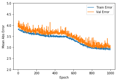

Observation
It can be seen that the mean absolute error is on an average about +/- 4.0. The validation error also is about the same. This can be reduced by playing around with the hyperparamaters and increasing the number of iterations
1a. Multivariate Regression in Tensorflow – R
# Install Tensorflow in RStudio
#install_tensorflow()
# Install Keras
#install_packages("keras")
library(tensorflow)library(keras)
library(dplyr)library(dummies)## dummies-1.5.6 provided by Decision Patternslibrary(tensorflow)
library(keras)Multivariate regression
This code performs multivariate regression using Tensorflow and keras on the advent of Parkinson disease through sound recordings see Parkinson Speech Dataset with Multiple Types of Sound Recordings Data Set. The clinician’s motorUPDRS score has to be predicted from the set of features.
Read the data
# Download the Parkinson's data from UCI Machine Learning repository
dataset <- read.csv("https://archive.ics.uci.edu/ml/machine-learning-databases/parkinsons/telemonitoring/parkinsons_updrs.data")

# Set the column names
names(dataset) <- c("subject","age", "sex", "test_time","motor_UPDRS","total_UPDRS","Jitter","Jitter.Abs",
                 "Jitter.RAP","Jitter.PPQ5","Jitter.DDP","Shimmer", "Shimmer.dB", "Shimmer.APQ3",
                 "Shimmer.APQ5","Shimmer.APQ11","Shimmer.DDA", "NHR","HNR", "RPDE", "DFA","PPE")

# Remove the column 'subject' as it is not relevant to analysis
dataset1 <- subset(dataset, select = -c(subject))

# Make the column 'sex' as a factor for using dummies
dataset1$sex=as.factor(dataset1$sex)
# Add dummy variables for categorical cariable 'sex'
dataset2 <- dummy.data.frame(dataset1, sep = ".")
## Warning in model.matrix.default(~x - 1, model.frame(~x - 1), contrasts =
## FALSE): non-list contrasts argument ignoreddataset3 <- na.omit(dataset2)Split the data as training and test in 80/20
## Split data 80% training and 20% test
sample_size <- floor(0.8 * nrow(dataset3))

## set the seed to make your partition reproducible
set.seed(12)
train_index <- sample(seq_len(nrow(dataset3)), size = sample_size)

train_dataset <- dataset3[train_index, ]
test_dataset <- dataset3[-train_index, ]

train_data <- train_dataset %>% select(sex.0,sex.1,age, test_time,Jitter,Jitter.Abs,Jitter.PPQ5,Jitter.DDP,
                              Shimmer, Shimmer.dB,Shimmer.APQ3,Shimmer.APQ11,
                              Shimmer.DDA,NHR,HNR,RPDE,DFA,PPE)

train_labels <- select(train_dataset,motor_UPDRS)
test_data <- test_dataset %>% select(sex.0,sex.1,age, test_time,Jitter,Jitter.Abs,Jitter.PPQ5,Jitter.DDP,
                              Shimmer, Shimmer.dB,Shimmer.APQ3,Shimmer.APQ11,
                              Shimmer.DDA,NHR,HNR,RPDE,DFA,PPE)
test_labels <- select(test_dataset,motor_UPDRS)
Normalize the data
 # Normalize the data by subtracting the mean and dividing by the standard deviation
normalize<-function(x) {
  y<-(x - mean(x)) / sd(x)
  return(y)
}

normalized_train_data <-apply(train_data,2,normalize)
# Convert to matrix
train_labels <- as.matrix(train_labels)
normalized_test_data <- apply(test_data,2,normalize)
test_labels <- as.matrix(test_labels)
Create the Deep Learning Model
model <- keras_model_sequential()
model %>%
  layer_dense(units = 6, activation = 'relu', input_shape = dim(normalized_train_data)[2]) %>%
  layer_dense(units = 9, activation = 'relu') %>%
  layer_dense(units = 6, activation = 'relu') %>%
  layer_dense(units = 1)

# Set the metrics required to be Mean Absolute Error and Mean Squared Error.For regression, the loss is
# mean_squared_error
model %>% compile(
  loss = 'mean_squared_error',
  optimizer = optimizer_rmsprop(),
  metrics = c('mean_absolute_error','mean_squared_error')
)

# Fit the model
# Use the test data for validation
history <- model %>% fit(
  normalized_train_data, train_labels,
  epochs = 30, batch_size = 128,
  validation_data = list(normalized_test_data,test_labels)
)
Plot mean squared error, mean absolute error and loss for training data and test data
plot(history)
Fig1

2. Binary classification in Tensorflow – Python
This is a simple binary classification problem from UCI Machine Learning repository and deals with data on Breast cancer from the Univ. of Wisconsin Breast Cancer Wisconsin (Diagnostic) Data Set bold text
import tensorflow as tf
from tensorflow import keras
import pandas as pd
# Read the data set from UCI ML site
dataset_path = keras.utils.get_file("breast-cancer-wisconsin.data", "https://archive.ics.uci.edu/ml/machine-learning-databases/breast-cancer-wisconsin/breast-cancer-wisconsin.data")
raw_dataset = pd.read_csv(dataset_path, sep=",", na_values = "?", skipinitialspace=True,)
dataset = raw_dataset.copy()

#Check for Null and drop
dataset.isna().sum()
dataset = dataset.dropna()
dataset.isna().sum()

# Set the column names
dataset.columns = ["id","thickness",	"cellsize",	"cellshape","adhesion","epicellsize",
                    "barenuclei","chromatin","normalnucleoli","mitoses","class"]
dataset.head()
Downloading data from https://archive.ics.uci.edu/ml/machine-learning-databases/breast-cancer-wisconsin/breast-cancer-wisconsin.data
24576/19889 [=====================================] - 0s 1us/step
id	thickness	cellsize	cellshape	adhesion	epicellsize	barenuclei	chromatin	normalnucleoli	mitoses	class
0	1002945	5	4	4	5	7	10.0	3	2	1	2
1	1015425	3	1	1	1	2	2.0	3	1	1	2
2	1016277	6	8	8	1	3	4.0	3	7	1	2
3	1017023	4	1	1	3	2	1.0	3	1	1	2
4	1017122	8	10	10	8	7	10.0	9	7	1	4
# Create a training/test set in the ratio 80/20
train_dataset = dataset.sample(frac=0.8,random_state=0)
test_dataset = dataset.drop(train_dataset.index)

# Set the training and test set
train_dataset1= train_dataset[['thickness','cellsize','cellshape','adhesion',
                'epicellsize', 'barenuclei', 'chromatin', 'normalnucleoli','mitoses']]
test_dataset1=test_dataset[['thickness','cellsize','cellshape','adhesion',
                'epicellsize', 'barenuclei', 'chromatin', 'normalnucleoli','mitoses']]
# Generate the stats for each column to be used for normalization
train_stats = train_dataset1.describe()
train_stats = train_stats.transpose()
train_stats
# Create target variables
train_labels = train_dataset.pop('class')
test_labels = test_dataset.pop('class')
# Set the target variables as 0 or 1
train_labels[train_labels==2] =0 # benign
train_labels[train_labels==4] =1 # malignant

test_labels[test_labels==2] =0 # benign
test_labels[test_labels==4] =1 # malignant
# Normalize by subtracting mean and dividing by standard deviation
def normalize(x):
  return (x - train_stats['mean']) / train_stats['std']

# Convert columns to numeric
train_dataset1 = train_dataset1.apply(pd.to_numeric)
test_dataset1 = test_dataset1.apply(pd.to_numeric)

# Normalize
normalized_train_data = normalize(train_dataset1)
normalized_test_data = normalize(test_dataset1)
# Create a model
model = tf.keras.Sequential([
    keras.layers.Dense(6, activation=tf.nn.relu, input_shape=[len(train_dataset1.keys())]),
    keras.layers.Dense(9, activation=tf.nn.relu),
    keras.layers.Dense(6,activation=tf.nn.relu),
    keras.layers.Dense(1)
  ])

# Use the RMSProp optimizer
optimizer = tf.keras.optimizers.RMSprop(0.01)

# Since this is binary classification use binary_crossentropy
model.compile(loss='binary_crossentropy',
                optimizer=optimizer,
                metrics=['acc'])


# Fit a model
history=model.fit(
  normalized_train_data, train_labels,
  epochs=1000, validation_data=(normalized_test_data,test_labels), verbose=0)
hist = pd.DataFrame(history.history)
hist['epoch'] = history.epoch
hist.tail()
# Plot training and test accuracy
plt.plot(history.history['acc'])
plt.plot(history.history['val_acc'])
plt.title('model accuracy')
plt.ylabel('accuracy')
plt.xlabel('epoch')
plt.legend(['train', 'test'], loc='upper left')
plt.ylim([0.9,1])
plt.show()


# Plot training and test loss
plt.plot(history.history['loss'])
plt.plot(history.history['val_loss'])
plt.title('model loss')
plt.ylabel('loss')
plt.xlabel('epoch')
plt.legend(['train', 'test'], loc='upper left')
plt.ylim([0,0.5])
plt.show()
# Plot training and test loss
plt.plot(history.history['loss'])
plt.plot(history.history['val_loss'])
plt.title('model loss')
plt.ylabel('loss')
plt.xlabel('epoch')
plt.legend(['train', 'test'], loc='upper left')
plt.ylim([0,0.5])
plt.show()

2a. Binary classification in Tensorflow -R
This is a simple binary classification problem from UCI Machine Learning repository and deals with data on Breast cancer from the Univ. of Wisconsin Breast Cancer Wisconsin (Diagnostic) Data Set
# Read the data for Breast cancer (Wisconsin)
dataset <- read.csv("https://archive.ics.uci.edu/ml/machine-learning-databases/breast-cancer-wisconsin/breast-cancer-wisconsin.data")

# Rename the columns
names(dataset) <- c("id","thickness",   "cellsize", "cellshape","adhesion","epicellsize",
                    "barenuclei","chromatin","normalnucleoli","mitoses","class")

# Remove the columns id and class
dataset1 <- subset(dataset, select = -c(id, class))
dataset2 <- na.omit(dataset1)

# Convert the column to numeric
dataset2$barenuclei <- as.numeric(dataset2$barenuclei)
Normalize the data
train_data <-apply(dataset2,2,normalize)
train_labels <- as.matrix(select(dataset,class))

# Set the target variables as 0 or 1 as it binary classification
train_labels[train_labels==2,]=0
train_labels[train_labels==4,]=1
Create the Deep Learning model
model <- keras_model_sequential()
model %>%
  layer_dense(units = 6, activation = 'relu', input_shape = dim(train_data)[2]) %>%
  layer_dense(units = 9, activation = 'relu') %>%
  layer_dense(units = 6, activation = 'relu') %>%
  layer_dense(units = 1)

# Since this is a binary classification we use binary cross entropy
model %>% compile(
  loss = 'binary_crossentropy',
  optimizer = optimizer_rmsprop(),
  metrics = c('accuracy')  # Metrics is accuracy
)
Fit the model. Use 20% of data for validation
history <- model %>% fit(
  train_data, train_labels,
  epochs = 30, batch_size = 128,
  validation_split = 0.2
)
Plot the accuracy and loss for training and validation data
plot(history)

3. MNIST in Tensorflow – Python
This takes the famous MNIST handwritten digits . It ca be seen that Tensorflow and Keras make short work of this famous problem of the late 1980s
# Download MNIST data
mnist=tf.keras.datasets.mnist
# Set training and test data and labels
(training_images,training_labels),(test_images,test_labels)=mnist.load_data()

print(training_images.shape)
print(test_images.shape)
# Plot a sample image from MNIST and show contents
import matplotlib.pyplot as plt
plt.imshow(training_images[1])
print(training_images[1])
[[ 0 0 0 0 0 0 0 0 0 0 0 0 0 0 0 0 0 0
0 0 0 0 0 0 0 0 0 0]
[ 0 0 0 0 0 0 0 0 0 0 0 0 0 0 0 0 0 0
0 0 0 0 0 0 0 0 0 0]
[ 0 0 0 0 0 0 0 0 0 0 0 0 0 0 0 0 0 0
0 0 0 0 0 0 0 0 0 0]
[ 0 0 0 0 0 0 0 0 0 0 0 0 0 0 0 0 0 0
0 0 0 0 0 0 0 0 0 0]
[ 0 0 0 0 0 0 0 0 0 0 0 0 0 0 0 51 159 253
159 50 0 0 0 0 0 0 0 0]
[ 0 0 0 0 0 0 0 0 0 0 0 0 0 0 48 238 252 252
252 237 0 0 0 0 0 0 0 0]
[ 0 0 0 0 0 0 0 0 0 0 0 0 0 54 227 253 252 239
233 252 57 6 0 0 0 0 0 0]
[ 0 0 0 0 0 0 0 0 0 0 0 10 60 224 252 253 252 202
84 252 253 122 0 0 0 0 0 0]
[ 0 0 0 0 0 0 0 0 0 0 0 163 252 252 252 253 252 252
96 189 253 167 0 0 0 0 0 0]
[ 0 0 0 0 0 0 0 0 0 0 51 238 253 253 190 114 253 228
47 79 255 168 0 0 0 0 0 0]
[ 0 0 0 0 0 0 0 0 0 48 238 252 252 179 12 75 121 21
0 0 253 243 50 0 0 0 0 0]
[ 0 0 0 0 0 0 0 0 38 165 253 233 208 84 0 0 0 0
0 0 253 252 165 0 0 0 0 0]
[ 0 0 0 0 0 0 0 7 178 252 240 71 19 28 0 0 0 0
0 0 253 252 195 0 0 0 0 0]
[ 0 0 0 0 0 0 0 57 252 252 63 0 0 0 0 0 0 0
0 0 253 252 195 0 0 0 0 0]
[ 0 0 0 0 0 0 0 198 253 190 0 0 0 0 0 0 0 0
0 0 255 253 196 0 0 0 0 0]
[ 0 0 0 0 0 0 76 246 252 112 0 0 0 0 0 0 0 0
0 0 253 252 148 0 0 0 0 0]
[ 0 0 0 0 0 0 85 252 230 25 0 0 0 0 0 0 0 0
7 135 253 186 12 0 0 0 0 0]
[ 0 0 0 0 0 0 85 252 223 0 0 0 0 0 0 0 0 7
131 252 225 71 0 0 0 0 0 0]
[ 0 0 0 0 0 0 85 252 145 0 0 0 0 0 0 0 48 165
252 173 0 0 0 0 0 0 0 0]
[ 0 0 0 0 0 0 86 253 225 0 0 0 0 0 0 114 238 253
162 0 0 0 0 0 0 0 0 0]
[ 0 0 0 0 0 0 85 252 249 146 48 29 85 178 225 253 223 167
56 0 0 0 0 0 0 0 0 0]
[ 0 0 0 0 0 0 85 252 252 252 229 215 252 252 252 196 130 0
0 0 0 0 0 0 0 0 0 0]
[ 0 0 0 0 0 0 28 199 252 252 253 252 252 233 145 0 0 0
0 0 0 0 0 0 0 0 0 0]
[ 0 0 0 0 0 0 0 25 128 252 253 252 141 37 0 0 0 0
0 0 0 0 0 0 0 0 0 0]
[ 0 0 0 0 0 0 0 0 0 0 0 0 0 0 0 0 0 0
0 0 0 0 0 0 0 0 0 0]
[ 0 0 0 0 0 0 0 0 0 0 0 0 0 0 0 0 0 0
0 0 0 0 0 0 0 0 0 0]
[ 0 0 0 0 0 0 0 0 0 0 0 0 0 0 0 0 0 0
0 0 0 0 0 0 0 0 0 0]
[ 0 0 0 0 0 0 0 0 0 0 0 0 0 0 0 0 0 0
0 0 0 0 0 0 0 0 0 0]]

# Normalize the images by dividing by 255.0
training_images = training_images/255.0
test_images = test_images/255.0

# Create a Sequential Keras model
model = tf.keras.models.Sequential([tf.keras.layers.Flatten(),
                                   tf.keras.layers.Dense(1024,activation=tf.nn.relu),
                                   tf.keras.layers.Dense(10,activation=tf.nn.softmax)])
model.compile(optimizer='adam',loss='sparse_categorical_crossentropy',metrics=['accuracy'])
history=model.fit(training_images,training_labels,validation_data=(test_images, test_labels), epochs=5, verbose=1)
Train on 60000 samples, validate on 10000 samples
Epoch 1/5
60000/60000 [==============================] - 17s 291us/sample - loss: 0.0020 - acc: 0.9999 - val_loss: 0.0719 - val_acc: 0.9810
Epoch 2/5
60000/60000 [==============================] - 17s 284us/sample - loss: 0.0021 - acc: 0.9998 - val_loss: 0.0705 - val_acc: 0.9821
Epoch 3/5
60000/60000 [==============================] - 17s 286us/sample - loss: 0.0017 - acc: 0.9999 - val_loss: 0.0729 - val_acc: 0.9805
Epoch 4/5
60000/60000 [==============================] - 17s 284us/sample - loss: 0.0014 - acc: 0.9999 - val_loss: 0.0762 - val_acc: 0.9804
Epoch 5/5
60000/60000 [==============================] - 17s 280us/sample - loss: 0.0015 - acc: 0.9999 - val_loss: 0.0735 - val_acc: 0.9812
Fig 1

Fig 2

MNIST in Tensorflow – R
The following code uses Tensorflow to learn MNIST’s handwritten digits ### Load MNIST data
mnist <- dataset_mnist()
x_train <- mnist$train$x
y_train <- mnist$train$y
x_test <- mnist$test$x
y_test <- mnist$test$y
Reshape and rescale
# Reshape the array
x_train <- array_reshape(x_train, c(nrow(x_train), 784))
x_test <- array_reshape(x_test, c(nrow(x_test), 784))
# Rescale
x_train <- x_train / 255
x_test <- x_test / 255
Convert out put to One Hot encoded format
y_train <- to_categorical(y_train, 10)
y_test <- to_categorical(y_test, 10)
Fit the model
Use the softmax activation for recognizing 10 digits and categorical cross entropy for loss
model <- keras_model_sequential()
model %>%
  layer_dense(units = 256, activation = 'relu', input_shape = c(784)) %>%
  layer_dense(units = 128, activation = 'relu') %>%
  layer_dense(units = 10, activation = 'softmax') # Use softmax

model %>% compile(
  loss = 'categorical_crossentropy',
  optimizer = optimizer_rmsprop(),
  metrics = c('accuracy')
)
Fit the model
Note: A smaller number of epochs has been used. For better performance increase number of epochs
history <- model %>% fit(
  x_train, y_train,
  epochs = 5, batch_size = 128,
  validation_data = list(x_test,y_test)
)
Plot the accuracy and loss for training and test data
plot(history)

Conclusion
This post shows how to use Tensorflow and Keras in both Python & R
Hope you have fun with Tensorflow!!
You may also like
1. My book ‘Practical Machine Learning in R and Python: Third edition’ on Amazon
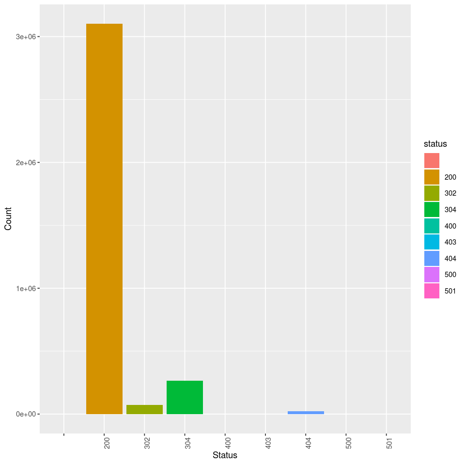
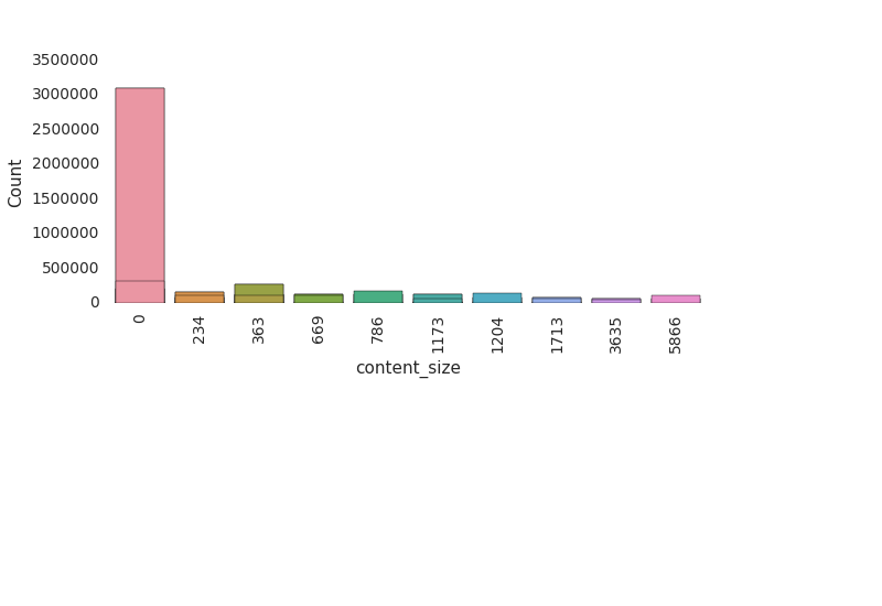
2. Big Data-4: Webserver log analysis with RDDs, Pyspark, SparkR and SparklyR
3. Deep Learning from first principles in Python, R and Octave – Part 5
4. Bend it like Bluemix, MongoDB using Auto-scale – Part 1!
5. A primer on Qubits, Quantum gates and Quantum Operations
6. Deblurring with OpenCV: Weiner filter reloaded
7. Introducing cricketr! : An R package to analyze performances of cricketers
8. Simulating a Web Joint in Android
9. Pitching yorkpy … short of good length to IPL – Part 1
To see all posts click Index of posts


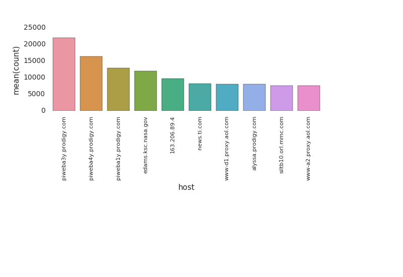
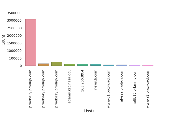


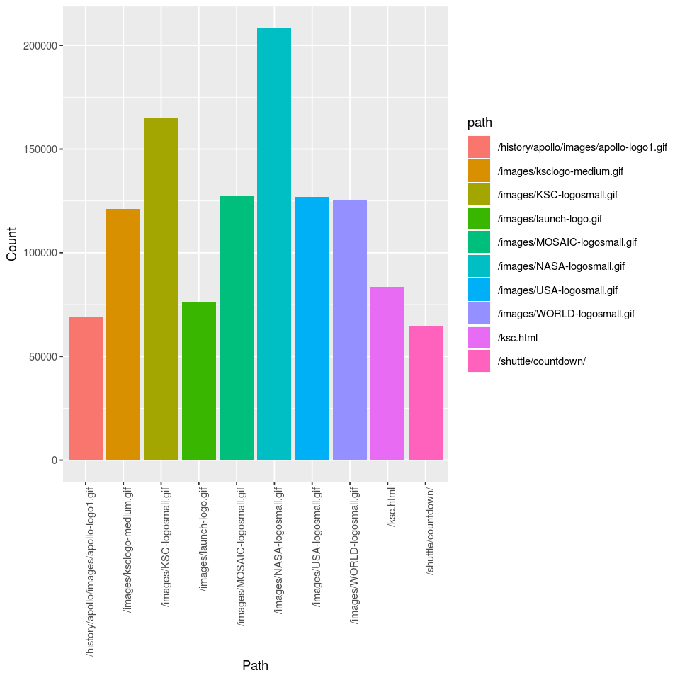


1.1 Read NASA Web server logs
Read the logs files from NASA for the months Jul 95 and Aug 95