How to program – Some essential tips

If one follows the arrow of time from the early 1980s to the present day, the number of programming problems have not only proliferated but have also become more difficult. Fortunately  programming in itself has  become more manageable with massive increases in computing horsepower, smarter tools and instant availability of information on the internet, typically with the click of a mouse.

Learning to program is no easy task, but can be done with the right mix of attitude, curiosity and interest. Becoming adept at programming, however, is something else. An interesting essay in this context is Peter Norvig’s ‘Teach yourself programming in 10 years’

Back in the 1980s when I wrote my first Fortran program on my college Mainframe, programming was a lengthy exercise, spanning several days.

1

My first program was to plot a sine wave of characters on a computer printout. Running this program required the following several steps

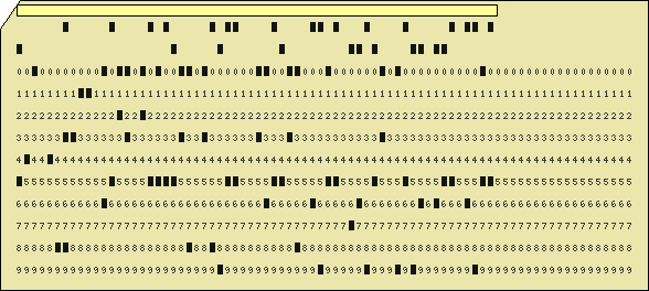
  1. Enter the program on a teletype terminal and create a stack of Hollerith (punched) cards
  2. Submit the stack of cards to the computer center
  3. The computer center would do a batch execute in the evening on the Mainframe
  4. God forbid, if your program has a syntax error. If you did find an error, go back to step 1, the next day.
  5. Assuming everything is fine, the computer center would run your program and your output (printout) would be placed in the appropriate pigeon hole which you would need to pick up the next day.

The whole exercise to write a small-sized program could take anywhere between a couple of days to a whole week.

In the early 1990s things got a little better where one could code, compile, link and execute sitting at one’s desk. However while the programming itself got much simpler than before, certain tasks were still difficult.  Till the late 90s programs of any sort had to be written using a regular text editor (vi , emacs etc.)  You would then have to go through the process of compiling, linking and executing.

An angry compiler would typically spew forth venom at missing semi-colons, undeclared variables, and uninitialized values. This would happen till you are able to iron out all syntax errors.  Then you would link, get undefined symbols and have to include appropriate libraries etc. And then finally you would execute your code, only to have it crash. The process of debugging would then start.

Luckily technology has made life a whole lot easier except for the last step where you could still  run into an execution errors . In these days an IDE (Interactive Development Environment) like Eclipse will flag syntax errors, missing definitions/declarations etc. as you write your code. Moreover Eclipse can also indicate which libraries (imports) you would need to include in your package for it to build. The only missing step in IDEs of these days is the ability to predict possible execution errors in your program.  I wouldn’t be surprised, if in future, like Microsoft Word,  the IDE is able to tell you if a programming construct does not make sense.

So things have gotten a lot easier for the programmer. The following tips for are particularly useful as you progress along in programming

  1. These days when you are learning a new programming language it is not necessary to know the language from cover to cover by reading a book. In those days when we learnt C it was necessary to know everything from bit structures, macros, pragma etc. The reason being that every syntax or execution error one had to rush to get the textbook and thumb through it for the answer. Not so, in these days of Google. You have the world’s library at your fingertips.
  2. To get started it is necessary to learn just the most important programming constructs of the language say structure, class, car, cdr besides the usual suspects like loops, conditions and case constructs
  3. Download and install an IDE for the language. In most case Eclipse will work
  4. Try to write a simple program and test out your code.
  5. To do any sort of programming these days you will necessarily need to make 3 friends
    1. Google
    2. Stackoverflow
    3. Git & GitHub
  6. Honing your Googling skills is very important. There are answers to almost any sort of programming problems out there. You would be surprised to know that there are many others who did exactly the same stupid mistake that you did out there. Also googling will take you to interesting tutorials, blogs, articles that discuss different aspects of the programming language and the problem you are trying to solve
  7. Stackoverflow is really a God send to all programmers. There are so many questions on so many aspects of every programming language on earth there. If you spend time searching Stackoverflow you are bound to find answers, code snippets that you can readily use in your code
  8. Post your questions in stackoverflow when you don’t find the answers there. You are bound to get quick answers. Thanks to the gamification of Stackoverflow (points, upvotes,badges  etc) that has been created on Stackoverflow.
  9. Git & GitHub: I would suggest that you download and install GitHub for Windows. This will provide you with version control on your desktop. You can modify code while being to switch back to an earlier version with Git. Read up a good tutorial on Git for Windows
  10. Once you have working code you push it onto GitHub and share with other programmers

Now that you have the basic setup here are few other extremely important tips

  1. The most important criteria for programming is ‘attitude’. Initially you are bound to get frustrated, angry, irritated etc. But it is necessary to look at the errors that you get with the right attitude. Know that an error is telling you something. Usually the answers to your mistake are in the ‘error message’ itself. Look at it closely and try to understand it. You will learn a lot more when you learn from errors than from copy-pasting from somebody else’s code, even if works right the first time around!
  2. Make sure you do something different each time. As Einstein said “ If you keep doing the same thing, you will keep getting the same result’
  3. There are different ways to debug your code. You could use the debugger and single step through the code and keep checking the values of the variables. I personally prefer print statements to localize where things are going wrong. I then try to narrow down the problem to a few lines of code and try to take it apart.

Hopefully the above tips are useful. Programming can be creative activity and will be indispensable in our future.

Above all have fun coding, there are so many possibilities these days!

Also see

1. Programming languages in layman’s language
2. The common alphabet of programming languages
3. The mind of the programmer
4. Programming Zen and now – Some essential tips -2 

You may also like
1. A crime map of India in R: Crimes against women
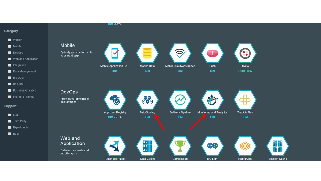
2.  What’s up Watson? Using IBM Watson’s QAAPI with Bluemix, NodeExpress – Part 1
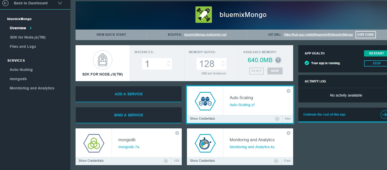
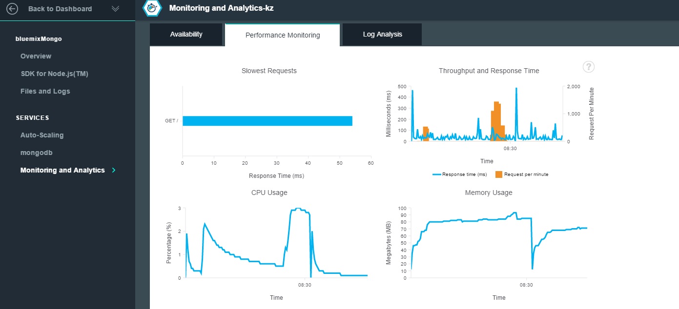
3.  Bend it like Bluemix, MongoDB with autoscaling – Part 2
4. Informed choices through Machine Learning : Analyzing Kohli, Tendulkar and Dravid
5. Thinking Web Scale (TWS-3): Map-Reduce – Bring compute to data
6. Deblurring with OpenCV:Weiner filter reloaded

Programming Zen and now – Some essential tips-2

Applying the principles of Machine Learning

While working with multivariate regression there are certain essential principles that must be applied to ensure the correctness of the solution while being able to pick the most optimum solution. This is all the more important when the problem has a large number of features. In this post I apply these important principles to a regression data set which I was able to pull of the internet. This data set was taken from the UCI Machine Learning repository and deals with Boston housing data.  The housing data provides the cost of house in Boston suburbs given the number of rooms, the connectivity to main highways, and crime rate in the area and several other data.  There are a total of 506 data points in this data set with a total of 13 features.

This seemed a reasonable dataset to start to try out the principles of Machine Learning I had picked up from Coursera’s ML course.

Out of a total of 13 features 2 features ’ZN’ and ‘CHAS’ proximity to  Charles river were dropped as the values were mostly zero in these columns . The remaining 11 features were used to map to the output variable of the price.

The following key rules have been applied on the

  • The dataset was divided into training samples (60%), cross-validation set (20%) and test set (20%) using a random index
  • Try out different polynomial functions while performing gradient descent to determine the theta values
  • Different combinations of ‘alpha’ learning rate and ‘lambda’ the regularization parameter were tried while performing gradient descent
  • The error rate is then calculated on the cross-validation and test set
  • The theta values that were obtained for the lowest cost for a polynomial was used to compute and plot the learning curve for the different polynomials against increasing number of training and cross-validation test samples to check for bias and variance.
  • The plot of the cost versus the polynomial degree was plotted to obtain the best fit polynomial for the data set.

A multivariate regression hypothesis can be represented as

hθ(x) = θ0 + θ1x1 + θ2x2 + θ3x3 + θ4x4 + …
And the cost can is determined as
J(θ0, θ1, θ2, θ3..) = 1/2m ∑ (hΘ (xi) -yi)2
The implementation was done using Octave. As in my previous posts some functions have not been include to comply with Coursera’s Honor Code. The code can be cloned from GitHub at machine-learning-principles

a) housing compute.m. In this module I perform gradient descent for different polynomial degrees and check the error that is obtained when using the computed theta on the cross validation and test set

max_degrees =4;
J_history = zeros(max_degrees, 1);
Jcv_history = zeros(max_degrees, 1);
for degree = 1:max_degrees;
[J Jcv alpha lambda] = train_samples(randidx, training,cross_validation,test_data,degree);
end;

b) train_samples.m – This module uses gradient descent to check the best fit for a given polynomial degree for different combinations of alpha (learning rate) and lambda( regularization).

for i = 1:length(alpha_arr),
for j = 1:length(lambda_arr)
alpha = alpha_arr{i};
lambda= lambda_arr{j};
% Perform Gradient descent
% Compute error for training sample for computed theta values
% Compute the error rate for the cross validation samples
% Compute the error rate against the test set
end;
end;

c) cross_validation.m – This module uses the theta values to compute cost for the cross validation set

d) test-samples.m – This modules computes the error when using the trained theta on the test set

e) poly.m – This module constructs polynomial vectors based on the degree as follows
function [x] = poly(xinput, n)
x = [];
for i= 1:n
xtemp = xinput .^i;
x = [x xtemp];
end;

e) learning_curve.m – The learning curve module plots the error rate for increasing number of training and cross validation samples. This is done as follows. For the theta with the lowest cost as determined by gradient descent
for i from 1 to 100

  • Compute the error for ‘i’ training samples
  • Compute the error for ‘i’ cross-validation
  • Plot the learning curve to determine the bias and variance of the polynomial fit

This is included below
for i = 1: 100
xsample = xtrain(1:i,:);
ysample = ytrain(1:i,:);
size(xsample);
size(ysample);
[xsample] = poly(xsample,degree);
xsample= [ones(i, 1) xsample];
[c d] = size(xsample);
theta = zeros(d, 1);
% Minimize using fmincg
J = computeCost(xsample, ysample, theta);
Jtrain(i) = J;
xsample_cv = xcv(1:i,:);
ysample_cv = ycv(1:i,:);
[xsample_cv] = poly(xsample_cv,degree);
xsample_cv= [ones(i, 1) xsample_cv];
J_cv = computeCost(xsample_cv, ysample_cv,theta)
Jcv(i) = J_cv;
end;

Finally a plot is done been different lambda and the cost.

The results are included below

A) Polynomial degree 1
Convergence graph
convergence-1

Learning curve
learning-curve-1

The above figure does show a stronger bias. Note: the learning curve was done with around 100 samples
B) Polynomial degree 2

Convergence graph
convergence-2

Learning curve
learning-curve-2

The learning curve for degree 2 shows a stronger variance.

C) Polynomial degree 3
Convergence graph

convergence-3

Learning curve
learning-curve-3

D) Polynomial degree 4
Convergence graph
convergence-4

E) Learning curve
learning-curve-4

This plot is useful to determine which polynomial degree will give the best fit for the dataset and the lowest cost

degree-cost-1

Clearly from the above it can be seen that degree 2 will give a good fit for the data set.

F) Lambda vs Cost function
lambda-cost-1

The above code demonstrates some key principles while performing multivariate regression
The code can be cloned from GitHub at machine-learning-principles

Informed choices through Machine Learning-2: Pitting together Kumble, Kapil, Chandra

Continuing my earlier ‘innings’, of test driving my knowledge in Machine Learning acquired via Coursera,  I now turn my attention towards the bowling performances of our Indian bowling heroes. In this post I give a slightly different ‘spin’ to the bowling analysis and hope I can ‘swing’ your opinion based on my assessment.

I guess that is enough of my cricketing ‘double-speak’ for now and I will get down to the real business of my bowling analysis!

If you are passionate about cricket, and love analyzing cricket performances, then check out my 2 racy books on cricket! In my books, I perform detailed yet compact analysis of performances of both batsmen, bowlers besides evaluating team & match performances in Tests , ODIs, T20s & IPL. You can buy my books on cricket from Amazon at $12.99 for the paperback and $4.99/$6.99 respectively for the kindle versions. The books can be accessed at Cricket analytics with cricketr  and Beaten by sheer pace-Cricket analytics with yorkr  A must read for any cricket lover! Check it out!!

1


As in my earlier post Informed choices through Machine Learning – Analyzing Kohli, Tendulkar and Dravid ,the first part of the post has my analyses and the latter part has the details of the implementation of the algorithm. Feel free to read the first part and either scan or skip the latter.

To perform this analysis I have skipped the data on our recent crop of new bowlers. The reason being that data is scant on these bowlers, besides they also seem to have a relatively shorter shelf life (hope there are a couple of finds in this Australian tour of Dec 2014). For the analyses I have chosen B S Chandrasekhar, Kapil Dev Anil Kumble. My rationale as to why I chose the above 3

B S Chandrasekhar also known as “Chandra’ was one of the most lethal leg spinners in the late 1970’s. He had a very dangerous combination of fast leg breaks, searing tops spins interspersed with the  occasional googly. On many occasions he would leave most batsmen completely clueless.

Kapil Nikhanj Dev, the Haryana Hurricane who could outwit the most technically sound batsmen  through some really clever bowling. His variations were almost always effective and he would achieve the vital breakthrough outsmarting the opponent.

And finally Anil Kumble, I chose Kumble because in my opinion he is truly the embodiment of the ‘thinking’ bowler. Many times I have seen Kumble repeatedly beat batsmen. It was like he was telling the batsman ‘check’ as he bowled faster leg breaks, flippers, a straighter delivery or top spins before finally crashing into the wickets or trapping the batsmen. It felt he was saying ‘checkmate dude!’

I have taken the data for the 3 bowlers from ESPN Cricinfo. Only the Test matches were considered for the analyses. All tests against all oppositions both at home and away were included

The assumptions taken and basis of the computation is included below
a.The data is based on the following 2 input variables a) Overs bowled b) Runs given. The output variable is ‘Wickets taken’

b.To my surprise I found that in the late 1970’s when BS Chandrasekhar used to bowl, an over had 8 balls for matches in Australia. So, I had to normalize this data for Chandra to make it on par with the others. Hence for Chandra where the overs were made up of 8 balls the overs was calculated as follows
Overs (O) = (Overs * 8)/6

c.The Economy rate E was calculated as below
E = Overs/runs was chosen as input variable to take into account fewer runs given by the bowler

d.The output variable was re-calculated as Strike Rate (SR) to determine the ‘bowling effectiveness’
Strike Rate = Wickets/Overs
(not be confused with a batsman’s strike rate batsman strike rate = runs/ balls faced)

e.Hence the analysis is based on
f(O,E) = SR
An outline of the Octave code and the data used can be cloned from GitHub at ml-bowling-analyze

 1. Surface of Bowling Effectiveness (SBE)
In my earlier post I was able to fit a ‘prediction plane’ based on the minutes at crease, balls faced versus the runs scored. But in this case a plane did not make sense as the wickets can only range from 0 – 10 and in most cases averaging between 3 and 5. So I plot the best fitting 3-D surface over the predicted hypothesis function. The steps performed are

1) The data for the different  bowlers were cleaned with data which indicated (DNB – Did not bowl)
2) The Economy Rate (E) = Runs given/Overs and Strike Rate(SR) = Wickets/overs were calculated.
3) The product of Overs (O), and Economy(E) were stored as Over_Economy(OE)
4) The hypothesis function was computed as h(O, E, OE) = y
5) Theta was calculated using the Normal Equation. The Surface of Bowling Effectiveness( SBE) was then plotted. The plots for each of the bowler is shown below

Here are the plots

A) Anil Kumble
The  data of Kumble, based on Overs bowled & Economy rate versus the Strike Rate is plotted as a 3-D scatter plot (pink crosses). The best fit as determined by solving the optimum theta using the Normal Equation is plotted as 3-D surface shown below.
kumble-1
The 3-D surface is what I have termed as ‘Surface of Bowling Effectiveness (SBE)’ as it depicts bowlers overall effectiveness as it plots the overs (O), ‘economy rate’ E against predicted ‘strike rate’ SR.
Here is another view
kumble-2
The theta values obtained for Kumble are
Theta =
0.104208
-0.043769
-0.016305
0.011949

And the cost at this theta is
Cost Function J = 0.0046269

B) B S Chandrasekhar
Here are the best optimal surface plot for Chandra with the data on O,E vs SR plotted as a 3D scatter plot.  Note: The dataset for  Chandrasekhar is smaller compared to the other two.
chandra-1Another view for Chandra
chandra-2

Theta values for B S Chandrasekhar are
Theta =
0.095780
-0.025377
-0.024847
0.023415
and the cost is
Cost Function J = 0.0032980

c) Kapil Dev
The plots  for Kapil
kapil-1
Another view of SBE for Kapil
kapil-2
The Theta values and cost function for Kapil are
Theta =
0.090219
0.027725
0.023894
-0.021434
Cost Function J = 0.0035123

2. Predicting wickets
In the previous section the optimum theta with the lowest Cost Function J was calculated. Based on the value of theta, the wickets that will be taken by a bowler can be computed as the product of the hypothesis function and theta. i.e.

y= h(x) * theta  => Strike Rate (SR) = [1 O E OE] * theta
Now predicted wickets can be calculated as

wickets = Strike rate(SR) * Overs(O)
This is done  for Kumble, Chandra and Kapil  for different combinations of Overs(O) and Economy(E) rate.

Here are the results
Predicted wickets for Anil Kumble
The plot of predicted wickets for Kumble is represented below
kumble-wickets-1
This can also be represented as a a table
kumble-wkts-tbl

Predicted wickets for B S Chandrasekhar
chandra-wickets-1
The table for Chandra
chandra-wkts-tbl
 Predicted wickets for Kapil Dev

The plot
kapil-wicket-2

The predicted table from the hypothesis function for Kapil Dev
kapil-wkts-tbl

Observation: A closer look at  the predicted wickets for Kapil, Kumble and B S Chandra shows an interesting aspect. The predicted number of wickets is higher for lower economy rates. With a little thought we can see bowlers on turning or pitches with a lot of movement can not only be more economical but can also be destructive and take a lot of wickets. Hence the higher wickets for lower economy rates!

Implementation details
In this post I have used the Normal Equation to get the optimal values of theta for local minimum of the Gradient function.  As mentioned above when I had run the 3D scatter plot fitting a 2D plane did not seem quite right. So I had to experiment with different polynomial equations first trying 2nd order, 3rd order and also the sqrt

I tried the following where ‘O is Overs, ‘E’ stands for Economy Rate and ‘SR’ the predicated Strike rate. Theta is the computed theta from the Normal Equation. The notation in  Matrix notation is shown below

i) A linear plane
SR = [1 O E] * theta

ii) Using the sqrt function
SR = [1 sqrt(O) sqrt(E)]  * theta

iii) Using 2nd order plynomial
SR = [1 O^2 E^2] * theta

iv) Using the 3rd order polynomial
SR = [1 O^3 E^3] * theta

v) Before finally settling on
SR = [1 O E OE] * theta

where OE  = O .* E

The last one seemed to give me the lowest cost and also seemed the most logical visual choice.

A good resource to play around with different functions and check out the shapes of combinations of variables and polynomial order of equation is at WolframAlpha: Plotting and Graphics

Note 1: The gradient descent with the Normal Equation has been performed on the entire data set (approx 220 for Kumble & Kapil) and 99 for Chandra. The proper process for verifying a Machine Learning algorithm is to split the data set into (60% training data, 20% cross validation data and 20% as the test set).  We need to validate the prediction function against the cross-validation set, fine tune it and finally ensure that it  fits  the test set samples well.  However, this split was not done as the data set itself was very low. The entire data set was used to perform the optimal surface fit

Note 2: The optimal theta values have been chosen with a feature vector that is of the form
[1 x y x .* y] The Surface of  Bowling Effectiveness’ has been plotted above. It may appear that there is a’high bias’ in the fit and an even better fit could be obtained by choosing higher order polynomials like
[1 x y x*y x^2 y^2 (x^2) .* y x  .* (y^2)] or
[1 x y x*y x^2 y^2 x^3 y^3]  etc
While we can get a better fit we could run into the problem of ‘high variance; and without the cross validation and test set we will not be able to verify the results, Hence the simpler option [1 x y x*y] was chosen

The Octave code outline and the data used can be cloned from GitHub at ml-bowling-analyze

 Conclusion:

1) Predicted wickets: The predicted number of wickets is higher at lower economy rates
2) Comparing performances: There are different ways of looking at the results. One possible way is to check for a particular number of overs and economy rate who is most effective. Here is one way. Taking a small slice from each bowler’s predicted wickets table for anm Economy Rate=4.0 the predicted wickets are

comp

From the above it does appear that Kapil is definitely more effective than the other two. However one could slice and dice in different ways, maybe the most economical for a given numbers and wickets combination or wickets taken in the least overs etc. Do add your thoughts. comments on my assessment or analysis

Also see
1. Analyzing cricket’s batting legends – Through the mirage with R
2. Masters of spin: Unraveling the web with R

You may also like
1. A peek into literacy in India:Statistical learning with R
2. A crime map of India in R: Crimes against women
3.  What’s up Watson? Using IBM Watson’s QAAPI with Bluemix, NodeExpress – Part 1

Informed choices through Machine Learning – Analyzing Kohli, Tendulkar and Dravid

Having just completed the highly stimulating & inspiring Stanford’s Machine Learning course at Coursera, by the incomparable Professor Andrew Ng I wanted to give my newly acquired knowledge a try. As a start, I decided to try my hand at  analyzing one of India’s fastest growing stars, namely Virat Kohli . For the data on Virat Kohli I used the ‘Statistics database’ at ESPN Cricinfo. To make matters more interesting,  I also pulled data on the iconic  Sachin Tendulkar and the Mr. Dependable,  Rahul Dravid.

If you are passionate about cricket, and love analyzing cricket performances, then check out my 2 racy books on cricket! In my books, I perform detailed yet compact analysis of performances of both batsmen, bowlers besides evaluating team & match performances in Tests , ODIs, T20s & IPL. You can buy my books on cricket from Amazon at $12.99 for the paperback and $4.99/$6.99 respectively for the kindle versions. The books can be accessed at Cricket analytics with cricketr  and Beaten by sheer pace-Cricket analytics with yorkr  A must read for any cricket lover! Check it out!!

1

(Also do check out my R package cricketr  Introducing cricketr! : An R package to analyze performances of cricketers and my interactive Shiny app implementation using my R package cricketr  – Sixer – R package cricketr’s new Shiny avatar )

Based on the data of these batsmen I perform some predictions with the help of machine learning algorithms. That I have a proclivity for prediction, is not surprising, considering the fact that my Dad was an astrologer who had reasonable success at this esoteric art. While he would be concerned with planetary positions, about Rahu in the 7th house being in the malefic etc., I on the other hand focus my  predictions on multivariate regression analysis and K-Means. The first part of my post gives the results of my analysis and some predictions for Kohli, Tendulkar and Dravid.

The second part of the post contains a brief outline of the implementation and not the actual details of implementation. This is ensure that I don’t violate Coursera’s Machine Learning’ Honor Code.

This code, data used and the output obtained  can be accessed at GitHub at ml-cricket-analysis

Analysis and prediction of Kohli, Tendulkar and Dravid with Machine Learning As mentioned above, I pulled the data for the 3 cricketers Virat Kohli, Sachin Tendulkar and Rahul Dravid. The data taken from Cricinfo database for the 3 batsman is based on  the following assumptions

  • Only ‘Minutes at Crease’ and ‘Balls Faced’ were taken as features against the output variable ‘Runs scored’
  • Only test matches were taken. This included both test ‘at home’ and ‘away tests’
  • The data was cleaned to remove any DNB (did not bat) values
  • No extra weightage was given to ‘not out’. So if Kohli made ‘28*’ 28 not out, this was taken to be 28 runs

 Regression Analysis for Virat Kohli There are 51 data points for Virat Kohli regarding Tests played. The data for Kohli is displayed as a 3D scatter plot where x-axis is ‘minutes’ and y-axis is ‘balls faced’. The vertical z-axis is the ‘runs scored’. Multivariate regression analysis was performed to find the best fitting plane for the runs scored based on the selected features of ‘minutes’ and ‘balls faced’.

This is based on minimizing the cost function and then performing gradient descent for 400 iterations to check for convergence. This plane is shown as the 3-D plane that provides the best fit for the data points for Kohli. The diagram below shows the prediction plane of  expected runs for a combination of ‘minutes at crease’ and ‘balls faced’. Here are 2 such plots for Virat Kohli. kohliAnother view of the prediction plane kohli-1 Prediction for Kohli I have also computed the predicted runs that will be scored by Kohli for different combinations of ‘minutes at crease’ and ‘balls faced’. As an example, from the table below, we can see that the predicted runs for Kohli   after being in the crease for 110 minutes  and facing 135 balls is 54 runs. kohli-score Regression analysis for Sachin Tendulkar There was a lot more data on Tendulkar and I was able to dump close to 329 data points. As before the ‘minutes at crease’, ‘balls faced’ vs ‘runs scored’ were plotted as a 3D scatter plot. The prediction plane is calculated using gradient descent and is shown as a plane in the diagram below srt Another view of this below srt-1 Predicted runs for Tendulkar The table below gives the predicted runs for Tendulkar for a combination of  time at crease and balls faced.  Hence,  Tendulkar will score 57 runs in 110 minutes after  facing 135 deliveries srt-score Regression Analysis for Rahul Dravid The same was done for ‘the Wall’ Dravid. The prediction plane is below dravid dravid-1 Predicted runs for Dravid The predicted runs for Dravid for combinations of batting time and balls faced is included below.  The predicted runs for Dravid after facing 135 deliveries in 110 minutes is 44. dravid-scoreFurther analysis While the ‘prediction plane’ was useful,  it somehow does not give a clear picture of how effective each batsman is. Clearly the 3D plots show at least 3 clusters for each batsman. For all batsmen, the clustering is densest near the origin, become less dense towards the middle and sparse on the other end. This is an indication during which session during their innings the batsman is most prone to get out. So I decided to perform K-Means clustering on the data for the 3 batsman. This gives the 3 general tendencies  for each batsman. The output is included below

K-Means for Virat The K-Means for Virat Kohli indicate the follow

Centroids found 255.000000 104.478261 19.900000
Centroids found 194.000000 80.000000 15.650000
Centroids found 103.000000 38.739130 7.000000

Analysis of Virat Kohli’s batting tendency
Kohli has a 45.098 percent tendency to bat for 104 minutes,  face 80 balls and score 38 runs
Kohli has a 39.216 percent tendency to bat for 19 minutes, face 15 balls and score 7 runs
Kohli has a 15.686 percent tendency to bat for 255 minutes, face 194 balls and score 103 runs

The computation of this included in the diagram below

kohli-kmeans

K-means for Sachin Tendulkar

The K-Means for Sachin Tendulkar indicate the following

Centroids found 166.132530 353.092593 43.748691
Centroids found 121.421687 250.666667 30.486911
Centroids found 65.180723 138.740741 15.748691

Analysis of Sachin Tendulkar’s performance

Tendulkar has a 58.232 percent tendency to bat for 43 minutes, face 30 balls and score 15 runs
Tendulkar has a 25.305 percent tendency to bat for 166 minutes, face 121 balls and score 65 runs
Tendulkar has a 16.463 percent tendency to bat for 353 minutes, face 250 balls and score 138 runs
srt-kmeans K-Means for Rahul Dravid

Centroids found 191.836364 409.000000 50.506024
Centroids found 137.381818 290.692308 34.493976
Centroids found 56.945455 131.500000 13.445783

Analysis of Rahul Dravid’s performance
Dravid has a 50.610 percent tendency to bat for 50 minutes,  face 34 balls and score 13 runs
Dravid has a 33.537 percent tendency to bat for 191 minutes,  face 137 balls and score 56 runs
Dravid has a 15.854 percent tendency to bat for 409 minutes, face 290 balls and score 131 runs
dravid-kmeans Some implementation details The entire analysis and coding was done with Octave 3.2.4. I have included the outline of the code for performing the multivariate regression. In essence the pseudo code for this

  1. Read the batsman data (Minutes, balls faced versus Runs scored)
  2. Calculate the cost
  3. Perform Gradient descent

The cost was plotted against the number of iterations to ensure convergence while performing gradient descent convergence-kohli Plot the 3-D plane that best fits the data
The outline of this code, data used and the output obtained  can be accessed at GitHub at ml-cricket-analysis

Conclusion: Comparing the results from the K-Means Tendulkar has around 48% to make a score greater than 60
Tendulkar has a 25.305 percent tendency to bat for 166 minutes, face 121 balls and score 65 runs
Tendulkar has a 16.463 percent tendency to bat for 353 minutes, face 250 balls and score 138 runs

And Dravid has a similar 48% tendency to score greater than 56 runs
Dravid has a 33.537 percent tendency to bat for 191 minutes,  face 137 balls and score 56 runs
Dravid has a 15.854 percent tendency to bat for 409 minutes, face 290 balls and score 131 runs

Kohli has around 45% to score greater than 38 runs
Kohli has a 45.098 percent tendency to bat for 104 minutes,  face 80 balls and score 38 runs

Also Kohli has a lesser percentage to score lower runs as against the other two
Kohli has a 39.216 percent tendency to bat for 19 minutes, face 15 balls and score 7 runs

The results must be looked in proper perspective as Kohli is just starting his career while the other 2 are veterans. Kohli has a long way to go and I am certain that he will blaze a trail of glory in the years to come!

Watch this space!

Also see
1. My book ‘Practical Machine Learning with R and Python’ on Amazon
2.Introducing cricketr! : An R package to analyze performances of cricketers
3.Informed choices with Machine Learning 2 – Pitting together Kumble, Kapil and Chandra
4. Analyzing cricket’s batting legends – Through the mirage with R
5. What’s up Watson? Using IBM Watson’s QAAPI with Bluemix, NodeExpress – Part 1
6. Bend it like Bluemix, MongoDB with autoscaling – Part 1


From developerWorks – What’s up, Watson? Using Watson QAAPI with Bluemix and NodeExpress

2

My post in IBM developer Works – What’s up, Watson? Using Watson QAAPI with Bluemix and NodeExpress

Create a Bluemix™ application that uses Watson’s Question and Answer API (QAAPI). IBM’s Watson is capable of understanding the nuances of the English language. Bluemix now includes eight services from Watson, including Concept Expansion, Language Identification, Machine Translation, and Question and Answer. For more information on Watson’s QAAPI and the many services that have been included in Bluemix, see Watson Services.

The current release of Bluemix Watson is a corpus of medical facts. Watson has been made to ingest medical documents in multiple formats (doc, pdf, html, text, and so on), and the user can pose medical questions to the Watson QAAPI.

This tutorial shows how to use the Watson Question and Answer API to make queries and get results of various types

n the application described in this tutorial, NodeExpress is used to create a web server and to post questions to Watson using REST APIs. Jade is used to format the results of Watson’s response.

For more details and the latest code please see my full article in IBM developerWorks What’s up, Watson? Using Watson QAAPI with Bluemix and NodeExpress

Bend it like Bluemix, MongoDB with auto-scaling – Part 3

In this last post of this series, I test the performance of Bluemix & MongoDB against  concurrent queries and deletes to the cloud based app with Mongo DB, with auto-scaling on. Before I started these series of tests I moved the Overload policy a couple of notches higher and made it scale out if  memory utilization > 75% for 120 secs and < 30% for 120 secs (from the earlier 55% memory utilization) as shown below.

27

The code for bluemixMongo app can be forked from Devops at bluemixMongo or can be cloned from GitHub at  bluemix-mongo-autoscale. The multi-mechanize scripts can be downloaded from GitHub at multi-mechanize     Before starting the testing I checked the current number of documents inserted by the concurrent inserts (see Bend it like Bluemix., MongoDB using Auto-scaling – Part 2). The total number as determined by checking the logs was 1380 17   Sure enough with the scaling policy change after 2 minutes the number of instanced dropped from 3 to 2

18

1. Querying the bluemixMongo app with Multi-mechanize

The Multi-mechanize Python script used for querying the bluemixMongo app simply invokes the app’s userlist URL (resp=br.open(“http://bluemixmongo.mybluemix.net/userlist/&#8221;)

v_user.py

def run(self):
# create a Browser instance
br = mechanize.Browser()
# don"t bother with robots.txt
br.set_handle_robots(False)
# start the timer
start_timer = time.time()
#print("Display userlist")
# Display 5 random documents
resp=br.open("http://bluemixmongo.mybluemix.net/userlist/")
assert("Example Mongo Page" in resp.get_data())
# stop the timer
latency = time.time() - start_timer
self.custom_timers["Userlist"] = latency
r = random.uniform(1, 2)
time.sleep(r)
self.custom_timers['Example_Timer'] = r

The configuration setup for this script creates 2 sets of 10 concurrent threads

config.cfg
run_time = 300
rampup = 0
results_ts_interval = 10
progress_bar = on
console_logging = off
xml_report = off
[user_group-1]
threads = 10
script = v_user.py
[user_group-2]
threads = 10
script = v_user.py

The corresponding userlist.js for querying the app is shown below. Here the query is constructed by creating a ‘RegularExpression’ with  a random Firstname, consisting of a random letter and a random number. Also the query is also limited to 5 documents.

function(callback)
{
// Display a random set of 5 records based on a regular expression made with random letter, number
var randnum = Math.floor((Math.random() * 10) + 1);
var alpha = ['A','B','C','D','E','F','G','H','I','J','K','L','M','N','O','P','Q','R','S','T','U','V','X','Y','Z'];
var randletter = alpha[Math.floor(Math.random() * alpha.length)];
var val =  randletter + ".*" + randnum + ".*";
// Limit the display to 5 documents
var results = collection.find({"FirstName": new RegExp(val)}).limit(5).toArray(function(err, items){
if(err) {
console.log(err + " Error getting items for display");
}
else {
res.render('userlist',
{ "userlist" : items
}); // end res.render
} //end else
db.close(); // Ensure that the open connection is closed
}); // end toArray function
callback(null, 'two');
}

2. Running the userlist query

The following screenshot shows the userlist query being executed concurrently with Multi-mechanize. Note that the number of  instances also drops down to 1

18

3. Deleting documents with Multi-mechanize

The multi-mechanize script for deleting a document is shown below. This script calls the URL with resp = br.open(“http://bluemixmongo.mybluemix.net/remuser&#8221;). No values are required to be entered into the form and the ‘submit’ is simulated.

v_user.py
def run(self):
# create a Browser instance
br = mechanize.Browser()
# don"t bother with robots.txt
br.set_handle_robots(False)
br.addheaders = [("User-agent", "Mozilla/5.0Compatible")]
# start the timer
start_timer = time.time()
# submit the request
resp = br.open("http://bluemixmongo.mybluemix.net/remuser")
#resp = br.open("http://localhost:3000/remuser")
resp.read()
# stop the timer
latency = time.time() - start_timer
# store the custom timer
self.custom_timers["Load_Front_Page"] = latency
# think-time
time.sleep(2)
# select first (zero-based) form on page
br.select_form(nr=0)
# set form field
br.form["firstname"] = ""
br.form["lastname"] = ""
br.form["mobile"] = ""
# start the timer
start_timer = time.time()
# submit the form
resp = br.submit()
resp.read()
print("Removed")
# stop the timer
latency = time.time() - start_timer
# store the custom timer
self.custom_timers["Delete"] = latency
# think-time
time.sleep(2)

config.cfg

The config file is set to start 2 sets of 10 concurrent threads and execute for 300 secs

[global]
run_time = 300
rampup = 0
results_ts_interval = 10
progress_bar = on
console_logging = off
xml_report = off
[user_group-1]
threads = 10
script = v_user.py
[user_group-2]
threads = 10
script = v_user.py
;

deleteuser.js

This Node.js script does a findOne() document and does a remove with the ‘justOne’ set to true

collection.findOne(function(err, item) {
// Delete just a single record
collection.remove(item, {justOne:true},(function (err, doc) {
if (err) {
// If it failed, return error
res.send("There was a problem removing the information to the database.");
}
else {
// If it worked redirect to userlist
res.location("userlist");
// And forward to success page
res.redirect("userlist");
}
}));
});
collection.find().toArray(function(err, items) {
console.log("Length =----------------" + items.length);
db.close();
});
callback(null, 'two');

4. Running the deleteuser multimechanize script

The output of the script executing and the reduction of the number of instances because of the change in the memory utilization policy is shown

21

5. Multi-mechanize

As mentioned in the previous posts

The multi-mechanize commands are executed as follows
To create a new project
multimech-newproject.exe userlist
This will create 2 folders a) results b) test_scripts and the file c) config.cfg. The v_user.py needs to be updated as required

To run the script
multimech-run.exe userlist

The details of the response times for the query is shown below .

All_Transactions_response_times_intervals


More details on latency and throughput for the queries and the deletes are included in the results folder of multi-mechanize    

6. Autoscaling The details of the auto-scaling service is shown below

a. Scaling Metric Statistics

22

b. Scaling history 23

7. Monitoring and Analytics (M & A) The output from M & A is shown  below


a. Performance Monitoring 24  

b. Log Analysis output The log analysis give a detailed report on the calls made to the app, the console log output and other useful information

25

The series of the 3 posts Bend it like Bluemix, MongoDB with auto-scaling demonstrated the ability of the cloud to expand and shrink based on the load on the cloud.An important requirement for Cloud Architects is design applications that can  scale horizontally without impacting the performance while keeping the costs optimum. The real challenge to auto-scaling is the need to make the application really distributed as opposed to the monolithic architectures we are generally used to.   I hope to write another post on creating simple distributed application later.

Hasta la Vista!

Also see
1.  Bend it like Bluemix, MongoDB with autoscaling – Part 1
2. Bend it like Bluemix, MongoDB with autoscaling – Part 2

You may like :
a) Latency, throughput implications for the cloud
b) The many faces of latency
c) Brewing a potion with Bluemix, PostgreSQL & Node.js in the cloud
d)  A Bluemix recipe with MongoDB and Node.js
e)Spicing up IBM Bluemix with MongoDB and NodeExpress
f) Rock N’ Roll with Bluemix, Cloudant & NodeExpress

Disclaimer: This article represents the author’s viewpoint only and doesn’t necessarily represent IBM’s positions, strategies or opinions

Bend it like Bluemix, MongoDB using Auto-scaling – Part 2!

This post takes off from my previous post Bend it like Bluemix, MongoDB using Auto-scale –  Part 1! In this post I generate traffic using Multi-Mechanize a performance test framework and check out the auto-scaling on Bluemix, besides also doing some rudimentary check on the latency and throughput for this test application. In this particular post I generate concurrent threads which insert documents into MongoDB.

Note: As mentioned in my earlier post this is more of a prototype and the typical situation when architecting cloud applications. Clearly I have not optimized my cloud app (bluemixMongo) for maximum efficiency. Also this a simple 2 tier application with a rudimentary Web interface and a NoSQL DB at This is more of a Proof of Concept (PoC) for the auto-scaling service on Bluemix.

As earlier mentioned the bluemixMongo app is a modification of my earlier post Spicing up a IBM Bluemix cloud app with MongoDB and NodeExpress. The bluemixMongo cloud app that was used for this auto-scaling test can be forked from Devops at bluemixMongo or from GitHib at bluemix-mongo-autoscale. The Multi-mechanize config file, scripts and results can be found at GitHub in multi-mechanize

The document to be inserted into MongoDB consists of 3 fields – Firstname, Lastname and Mobile. To simulate the insertion of records into MongoDB I created a Multi-Mechanize script that will generate random combination of letters and numbers for the First and Last names and a random 9 digit number for the mobile. The code for this script is shown below

1. The snippet below measure the latency for loading the ‘New User’ page

v_user.py
def run(self):
# create a Browser instance
br = mechanize.Browser()
# don"t bother with robots.txt
br.set_handle_robots(False)
print("Rendering new user")
br.addheaders = [("User-agent", "Mozilla/5.0Compatible")]
# start the timer
start_timer = time.time()
# submit the request
resp = br.open("http://bluemixmongo.mybluemix.net/newuser")
#resp = br.open("http://localhost:3000/newuser")
resp.read()
# stop the timer
latency = time.time() - start_timer
# store the custom timer
self.custom_timers["Load Add User Page"] = latency
# think-time
time.sleep(2)

The script also measures the time taken to submit the form containing the Firstname, Lastname and Mobile

# select first (zero-based) form on page
br.select_form(nr=0)
# Create random Firstname
a = (''.join(random.choice(string.ascii_uppercase) for i in range(5)))
b = (''.join(random.choice(string.digits) for i in range(5)))
firstname = a + b
# Create random Lastname
a = (''.join(random.choice(string.ascii_uppercase) for i in range(5)))
b = (''.join(random.choice(string.digits) for i in range(5)))
lastname = a + b
# Create a random mobile number
mobile = (''.join(random.choice(string.digits) for i in range(9)))
# set form field
br.form["firstname"] = firstname
br.form["lastname"] = lastname
br.form["mobile"] = mobile
# start the timer
start_timer = time.time()
# submit the form
resp = br.submit()
print("Submitted.")
resp.read()
# stop the timer
latency = time.time() - start_timer
# store the custom timer
self.custom_timers["Add User"] = latency

2. The config.cfg file is setup to generate 2 asynchronous thread pools of 10 threads for about 400 seconds

config.cfg
run_time = 400
rampup = 0
results_ts_interval = 10
progress_bar = on
console_logging = off
xml_report = off
[user_group-1]
threads = 10
script = v_user.py
[user_group-2]
threads = 10
script = v_user.py

3. The code to add a new user in the app (adduser.js) uses the ‘async’ Node module to enforce sequential processing.

adduser.js
async.series([
function(callback)
{
collection = db.collection('phonebook', function(error, response) {
if( error ) {
return; // Return immediately
}
else {
console.log("Connected to phonebook");
}
});
callback(null, 'one');
},
function(callback)
// Insert the record into the DB
collection.insert({
"FirstName" : FirstName,
"LastName" : LastName,
"Mobile" : Mobile
}, function (err, doc) {
if (err) {
// If it failed, return error
res.send("There was a problem adding the information to the database.");
}
else {
// If it worked, redirect to userlist - Display users
res.location("userlist");
// And forward to success page
res.redirect("userlist")
}
});
collection.find().toArray(function(err, items) {
console.log("**************************>>>>>>>Length =" + items.length);
db.close(); // Make sure that the open DB connection is close
});
callback(null, 'two');
}
]);

4. To checkout auto-scaling the instance memory was kept at 128 MB. Also the scale-up policy was memory based and based on the memory of the instance exceeding 55% of 128 MB for 120 secs. The scale up based on CPU utilization was to happen when the utilization exceed 80% for 300 secs.

6

5. Check the auto-scaling policy

7

6. Initially as seen there is just a single instance

9

7. At around 48% of the script with around 623 transactions the instance is increased by 1. Note that the available memory is decreased by 640 MB – 128 MB = 512 MB.

10

8. At around 1324 transactions another instance is added

Note: Bear in mind

a) The memory threshold was artificially brought down to 55% of 128 MB.b) The app itself is not optimized for maximum efficiency

12

9. The Metric Statistics tab for the Autoscaling service shows this memory breach and the trigger for autoscaling

13

10. The Scaling history Tab for the Auto-scaling service displays the scale-up and scale-down and the policy rules based on which the scaling happened

14

11. If you go to the results folder for the Multi-mechanize tool the response and throughput are captured.

The multi-mechanize commands are executed as follows
To create a new project
multimech-newproject.exe adduser
This will create 2 folders a) results b) test_scripts and the file c) config.cfg. The v_user.py needs to be updated as required

To run the script
multimech-run.exe adduser

12.The results are shown below

a) Load Add User page (Latency)

Load Add User Page_response_times_intervals

b) Load Add User (Throughput)

Load Add User Page_throughput

c)Load Add User (Latency)

Add User_response_times_intervals

d) Load Add User (Throughput)

Add User_throughput

The detailed results can be seen at GitHub at multi-mechanize

13. Check the Monitoring and Analytics Page

a) Availability

16

b) Performance monitoring

15

So once the auto-scaling happens the application can be fine-tuned and for performance. Obviously one could do it the other way around too.

As can be seen adding NoSQL Databases like MongoDB, Redis, Cloudant DB etc. Setting up the auto-scaling policy is also painless as seen above.

Of course the real challenge in cloud applications is to make them distributed and scalable while keeping the applications themselves lean and mean!

See also

Also see
1.  Bend it like Bluemix, MongoDB with autoscaling – Part 1
3. Bend it like Bluemix, MongoDB with autoscaling – Part 3

You may like :
a) Latency, throughput implications for the cloud
b) The many faces of latency
c) Brewing a potion with Bluemix, PostgreSQL & Node.js in the cloud
d)  A Bluemix recipe with MongoDB and Node.js
e)Spicing up IBM Bluemix with MongoDB and NodeExpress
f) Rock N’ Roll with Bluemix, Cloudant & NodeExpress

a) Latency, throughput implications for the cloud

b) The many faces of latency

c) Design principles of scalable, distributed systems

Disclaimer: This article represents the author’s viewpoint only and doesn’t necessarily represent IBM’s positions, strategies or opinions

Bend it like Bluemix, MongoDB using Auto-scale – Part 1!

In the next series of posts I turn on the heat on my cloud deployment in IBM Bluemix and check out the elastic nature of this PaaS offering. Handling traffic load and elastically expanding and contracting is what the cloud does best. This is  where the ‘rubber really meets the road”. In this series of posts I generate the traffic load using Multi –Mechanize a performance test framework created by Corey Goldberg.

This post is based on an earlier cloud app that I created on Bluemix namely Spicing up a IBM Bluemix Cloud app with MongoDB and NodeExpress. I had to make changes to this code to iron out issues while handling concurrent  inserts, displays and deletes issued from the multi-mechanize tool and also to manage the asynchronous nightmare of Nodejs.

The code for this Bluemix, MongoDB with Auto-scaling can be forked  from Devops at bluemixMongo. The code can also be cloned from GitHub at bluemix-mongo-autoscale

1.  To get started, fork the code from Devops at bluemixMongo. Then change the host name in manifest.yml to something unique and click the Build and Deploy button on the top right in the page.

26

1a.  Alternatively the code can be cloned from GitHub at bluemix-mongo-autoscale. From the directory where the code is cloned push the code using Cloud Foundry’s cf command as follows

cf login -a https://api.ng.bluemix.net

cf push bluemixMongo –p . –m 128M

2. Now add the MongoDB service and click ‘OK’ to restage the server.

3

3. Add the Monitoring and Analytics (M & A) and also the Auto-scaling service. The M& A gives a good report on the Availability, Performance logging, and also provides Logging Analysis. The Auto-scaling service is the service that allows the app to expand elastically to changing traffic loads.

4

4. You should see the bluemixMongo app running with 3 services MongoDB, Autoscaling and M&A

5

5. You should now be able click the bluemixMongo.mybluemix.net and check the application out.

6.Now you configure the Overload Policy (auto scaling) policy. This is a slightly contrived example and the scaling policy is set to scale up if the Memory exceeds 55%. (Typically the scale up would be configured for > 80% memory usage)

6

7. Now check the configured Auto-scaling policy

7

8. Change the Memory Quota as appropriate. In my case I have kept the memory quota as 128 MB. Note the available memory is 640 MB and hence allows up to 5 instances. (By the way it is also possible to set any other value like 100 MB).

5

9. Click the Monitoring and Analytics service and take a look at the output in the different tabs

8

10. Next you need to set up the Performance test tool – Multi mechanize. Multi-mechanize creates concurrent threads to generate the load on a Web site or service. It is based on Python which  makes it easy to modify the scripts for hitting a website, making a REST call or submitting a form.

To setup Multi-mechanize you also need additional packages like numpy  matplotlib etc as the tool generates traffic based on a user provided script, measures latency and throughput besides also generating graphs for these.

For a detailed steps for setup of Multi mechanize please follow the steps in Trying out multi-mechanize web performance and load testing framework. Note: I would suggest that you install Python 2.7.2 and not the later 3.x version as some of the packages are based on the 2.7 version which has a slightly different syntax for certain Python statements

In the next post I will run a traffic test on the bluemixMongo application using Multi-mechanize and observe how the cloud app responds to the load.

Watch this space!
Also see
Bend it like Bluemix, MongoDB with autoscaling – Part 2!
Bend it like Bluemix, MongoDB with autoscaling – Part 3

You may like :
a) Latency, throughput implications for the cloud
b) The many faces of latency
c) Brewing a potion with Bluemix, PostgreSQL & Node.js in the cloud
d)  A Bluemix recipe with MongoDB and Node.js
e)Spicing up IBM Bluemix with MongoDB and NodeExpress
f) Rock N’ Roll with Bluemix, Cloudant & NodeExpress

Disclaimer: This article represents the author’s viewpoint only and doesn’t necessarily represent IBM’s positions, strategies or opinions

Where is the Cloud Computing bus going?

delorean_19813Technological innovation patterns have often repeated themselves in history. So it is with Cloud Computing. Familiar patterns of change seem to emerge today

Here are some of main trends that I see in Cloud Computing

Advent of containers: Containers are the new hot topic in cloud computing. In virtualization guest OS’es run separately. Running separate guest OS over the hypervisor is associated with a lot of overhead for each of the heavy weight OS’es. Containers can be used as an alternative to OS-level virtualization to run multiple isolated systems on a single host. Containers within a single operating system are much more efficient being light weight while being able to provide the same level of isolation. Containers run the same kernel as the host. Here is an interesting article on containers Containers, not virtual machines are the future of the cloud.

In many ways this containers over VM innovation pattern is reminiscent of the advantages of lightweight ‘threads’ over the heavy and slow ‘process’ approach in the OS world.  It is inevitable that containers will eventually score over VMs

Open ‘something’ over proprietary’ness: Technology over the decades has always moved into an ‘open’ approach over proprietary solutions. Hence, for example, we have OpenStack for creating instances, provisioning storage, network to do many things that are being done separately by VMWare, Citrix, Hyper-V. The intent is to have a common approach over several disparate approaches. In the networking world there is OpenFlow which tries to have a uniform interface to the many different standards maintained by the Ciscos, Junipers and Brocades of the world.  There are also other technologies like OpenCV (Computer Vision processing), Open VPN (VPN protocol) etc. In all these approaches there is either to move to unify or to provide a layer over and above the disparate approaches.  I am not sure whether Openstack will prevail, only time will tell. I personally think we will move to a level abstraction that will be even above that of Open Stack.

Software Defined Everything: Cloud Computing started with the need to be able to provision computing resources through a user interface or the Web portal. This was made possible, thanks to virtualization. Users could now define and request computing resources. Soon this led to the need for being able to programmatically request storage. The trick in storage is to do ‘thin-provisioning’ or to provision resources that barely satisfies the needs of the application. The application will be able to request more storage programmatically. Not to be outdone, networking followed suit when Software Defined Networking became a reality when Stanford and University of California came with the Open Flow protocol. We have now entered into the era of Software Defined Datacenter. This is a dominant theme in Cloud Computing.

These are some of the predominant trends that are emerging in the Cloud Computing arena.

I have spent more than 2 decades of my career in telecom, implementing telecom protocols, starting in the mid-1980s. The mid 1980s was the time when digital switches started to emerge. This was followed by a spate of protocols and dizzying innovations like mobile telephony, ISDN, Intelligent Networks, Softswitch, UMTS,3G, HSDPA, LTE etc.

I personally think that Cloud computing, to use a very frayed and hackneyed term, is at a similar ‘inflexion point’. Trends are emerging and we will soon be caught in the maelstrom of rapid change and innovation.

In this post I am going to do a Marty McFly of the ‘Back to Future’ trilogy. I am going to set the clock of the Delorean DMC-12 to 2020 and ‘Whoosh…..’

21 Apr 2020:

It is 21 Apr 2020 and a sunny day.  Here is a look at the Cloud Computing landscape

  • The Organization of Cloud Computing Standards (OCCS) now sets and governs the standards for all Cloud Providers of the world
  • Common APIs govern provisioning of instances on the cloud regardless of the Cloud Provider. Instances are defined by RPE values, RAM and IOPS, LB, DNS requirements
  • Networking bandwidth, security and storage are also standards based
  • Enterprises use a ‘diffuse deployment’ strategy where the organization’s workloads are deployed to multiple cloud providers.
  • Workloads are Cloud Provider agnostic.
  • Enterprise applications themselves may span multiple cloud providers for e.g. the e-commerce in Cloud Provider 1, Analytics on HPC instances on Cloud Provider 2 and secure applications on Private Cloud of Cloud Provider 3. Appropriate contracts are maintained between the Cloud Providers for charging for the usage.
  • Algorithms are used by enterprises to deploy workloads to cloud providers. The algorithms match the SLA and cost requirements of the application with those offered by the cloud provider to minimize the cost while meeting the SLA requirements of the applications.
  • Compute, storage and networking costs fluctuate and enterprises use algorithms to optimize the deployment of workloads. Workloads are migrated to take advantage of these price changes
  • Consolidation and acquisitions happen at an alarming pace. Cloud providers, storage, network and HPC providers aslo compete fiercely
  • Cloud providers are swallowed by others and some lose out. The battle scene is bloody

Time to get back to Delorean. This time the clock on Delorean is set to 2025

18 Sep 2025

Today it is 18 Sep 2025, and it is sunny again, coincidentally.

  • Cloud Computing is dead, mate. These days technology has moved to ‘Cloud Computing in a box’.
  • The technology of these times are ‘Haze works’ where the computation happens in the stratosphere over the ether …

So much for looking into the future. It is now time to get back to the reality of VMs