Cricketr analyzes Ind-Aus faceoff in WTC 2023!!

“The unexamined life is not worth living.” – Socrates

“There is no easy way from the earth to the stars.” – Seneca

“If you want to go fast, go alone. If you want to go far, go together.” – African Proverb

1. Introduction

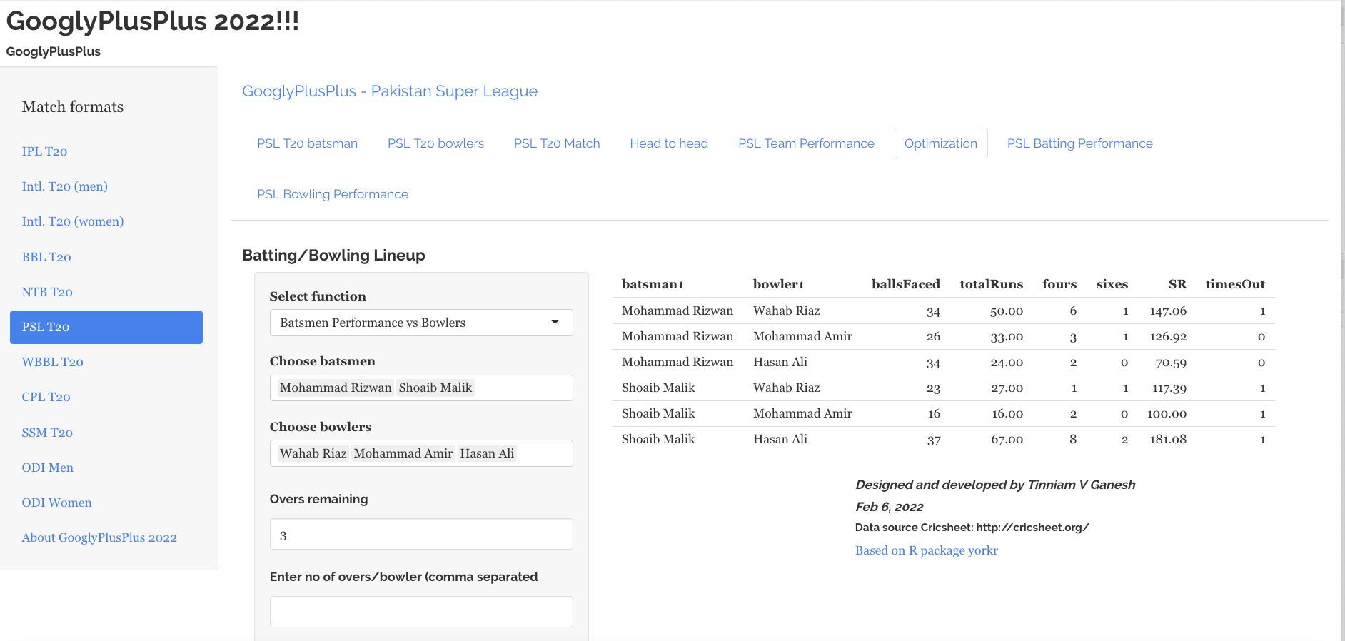
In this post, I put my R package cricketr to analyze the Indian and Australia World Test Championship (WTC) final squad ahead of the World Test Championship 2023.My R package cricketr had its birth on Jul 4, 2015. Cricketr uses data from Cricinfo.

You can download the latest PDF version of the book at ‘Cricket analytics with cricketr and cricpy: Analytics harmony with R and Python-6th edition‘

Indian squad

Rohit Sharma (Captain), Shubman Gill, Cheteshwar Pujara, Virat Kohli, Ajinkya Rahane, Ravindra Jadeja, Shardul Thakur, Mohd. Shami, Mohd. Siraj, Ishan Kishan (wk).

According to me, Ishan Kishan has more experience than KS Bharat, though Rishabh Pant would have been the ideal wicket keeper/left-handed batsman. I think Shardul Thakur would be handful in the English conditions. For a spinner it either Ashwin or Jadeja. Maybe the balance shifts in favor of Jadeja

Australian squad

Pat Cummins (capt), Alex Carey (wk), Cameron Green, Josh Hazlewood, Usman Khawaja, Marnus Labuschagne, Nathan Lyon, Todd Murphy, Steven Smith (vice-capt), Mitchell Starc, David Warner.

Not sure if Scott Boland would fill in, instead of Todd Murphy 1

Let me give you a lay-of-the-land (post) below

The post below is organized into the following parts

Analysis of Indian WTC batsmen from Jan 2016 – May 2023
Analysis of Indian WTC batsmen against Australia from Jan 2016 -May 2023
Analysis of Australian WTC batsmen from Jan 2016 – May 2023
Analysis of Australian WTC batsmen against India from Jan 2016 -May 2023
Analysis of Indian WTC bowlers from Jan 2016 – May 2023
Analysis of Indian WTC bowlers against Australia from Jan 2016 -May 2023
Analysis of Australian WTC bowlers from Jan 2016 – May 2023
Analysis of Australian WTC bowlers gainst India from Jan 2016 -May 2023
Team analysis of India and Australia

All the above analysis use data from ESPN Statsguru and use my R pakage cricketr

The data for the different players have been obtained using calls such as the ones below.

# Get Shubman Gill's batting data
#shubman <-getPlayerData(1070173,dir=".",file="shubman.csv",type="batting",homeOrAway=c(1,2), result=c(1,2,4))
#shubmansp <- getPlayerDataSp(1070173,tdir=".",tfile="shubmansp.csv",ttype="batting")

#Get Shubman Gill's data from Jan 2016 - May 2023
#df <-getPlayerDataHA(1070173,tfile="shubman1.csv",type="batting", matchType="Test")
#df1=getPlayerDataOppnHA(infile="shubman1.csv",outfile="shubmanTestAus.csv",startDate="2016-01-01",endDate="2023-05-01")

#Get Shubman Gills data from Jan 2016 - May 2023, against Australia
#df <-getPlayerDataHA(1070173,tfile="shubman1.csv",type="batting", matchType="Test")
#df1=getPlayerDataOppnHA(infile="shubman1.csv",outfile="shubmanTestAus.csv",opposition="Australia",startDate="2016-01-01",endDate="2023-05-01")

Note: To get data for bowlers we need to use the corresponding profile no and use type =‘bowling’. Details in my posts below

To do similar analysis please go through the following posts

Note 1: I will not be analysing each and every chart as the charts are quite self-explanatory

Note 2: I have had to tile charts together otherwise this will become a very, very long post. You are free to use my R package cricketr and check out for yourself ##3. Analysis of India WTC batsmen from Jan 2016 – May 2023

Findings

Kohli has the best average of 48+. India has won when Rohit and Rahane played well
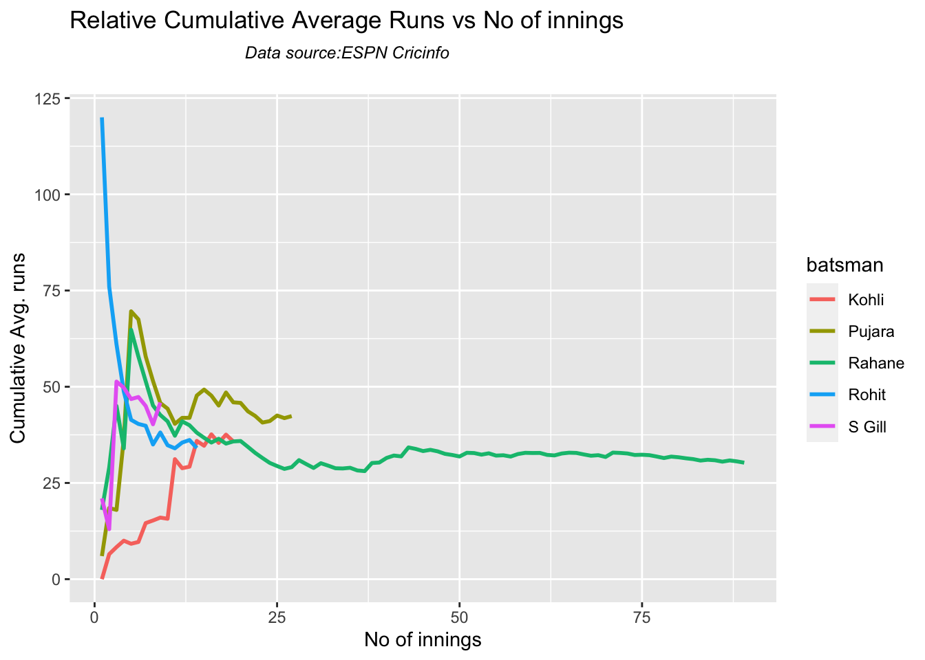
Kohli’s tops the list in cumulative average runs, followed by Pujara and Rohit is 3rd. Gill is on the upswing.
Against Australia Pujara has the best cumulative average runs record followed by Rahane, with Gill in hot pursuit. In the strike rate department Gill tops followed by Rohit and Rahane
Since 2016 Smith, Labuschagne has an average of 53+ since 2016!! Warner & Khwaja are at ~46
Australia has won matches when Smith, Warner and Khwaja have played well.
Labuschagne, Smith and C Green have good records against India. Indian bowlers will need to contain them
Ashwin has the highest wickets followed by Jadeja against all teams. Ashwin’s performance has dropped over the years, while Siraj has been becoming better
Jadeja has the best economy rate followed by Ashwin
Against Australia specifically Jadeja has the best record followed by Ashwin. Jadeja has the best economy against Australia, followed by Siraj, then Ashwin
Cummins, Starc and Lyons are the best performers for Australia. Hazzlewood, Cummins have the best economy against all opposition
Against India Lyon, Cummins and Hazzlewood have performed well
Hazzlewood, Lyon have a good economy rate against India
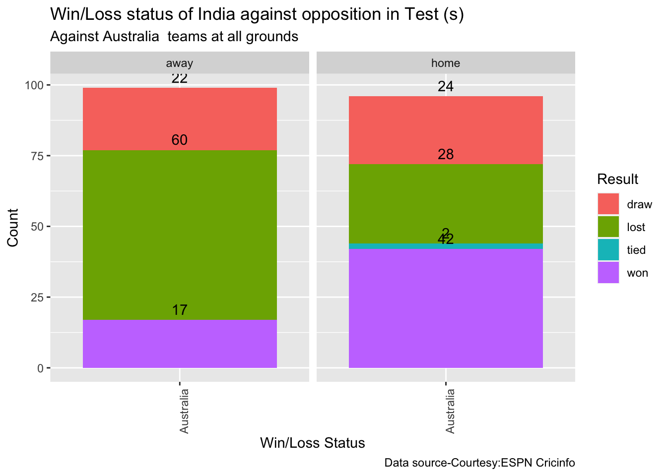
Against Australia India has won 17 times, lost 60 and drawn 22 in Australia. At home India won 42, tied 2, lost 28 and drawn 24
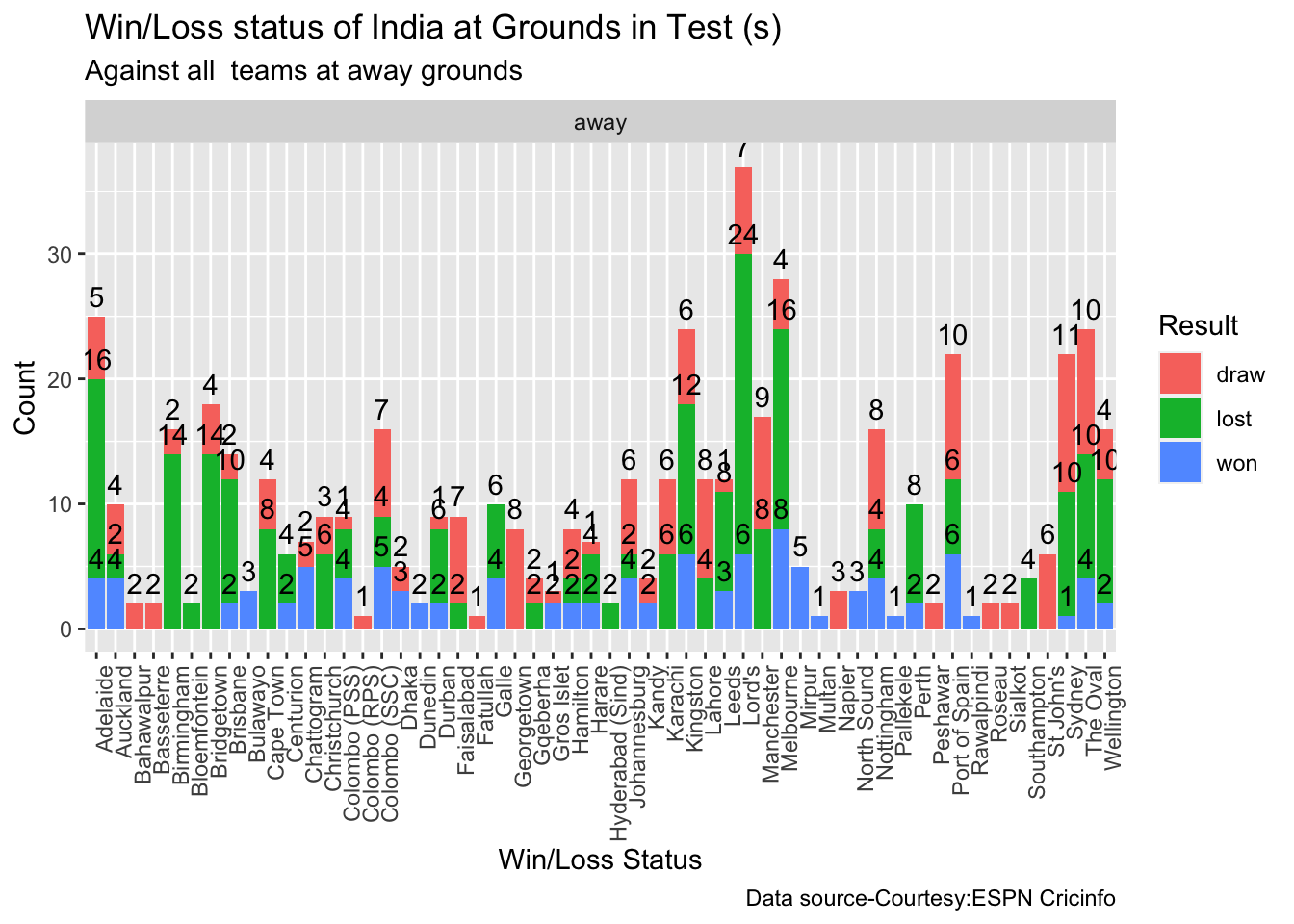
At the Oval where the World Test Championship is going to be held India has won 4, lost 10 and drawn 10.

Note 3: You can also read this post at Rpubs at ind-aus-WTC !! The formatting will be nicer!

Note 4: You can download this post as PDF to read at your leisure ind-aus-WTC.pdf

2. Install the cricketr package

if (!require("cricketr")){
    install.packages("cricketr",lib = "c:/test")
}
library(cricketr)

3a. Basic analysis

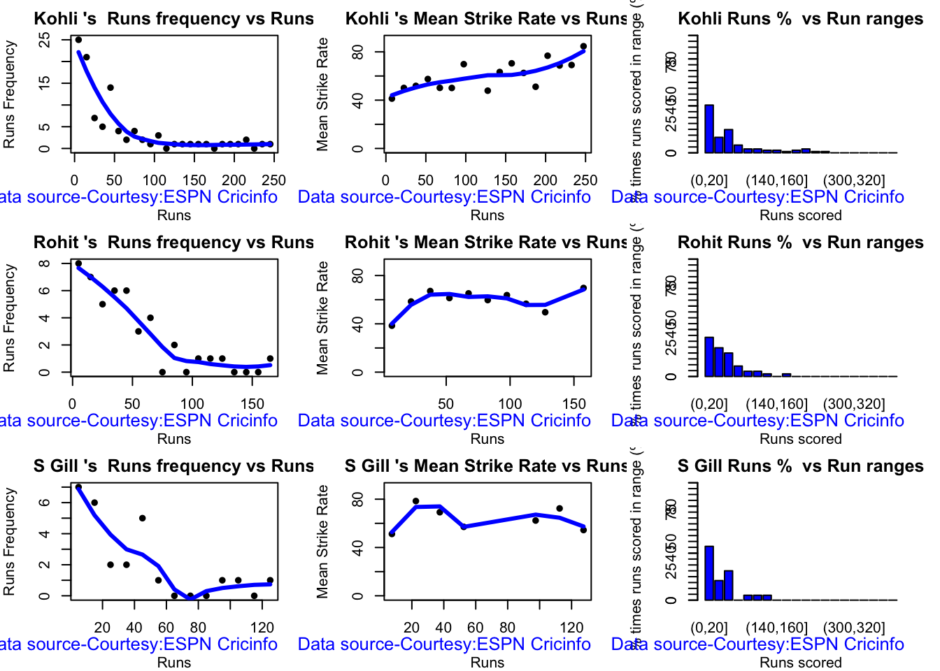
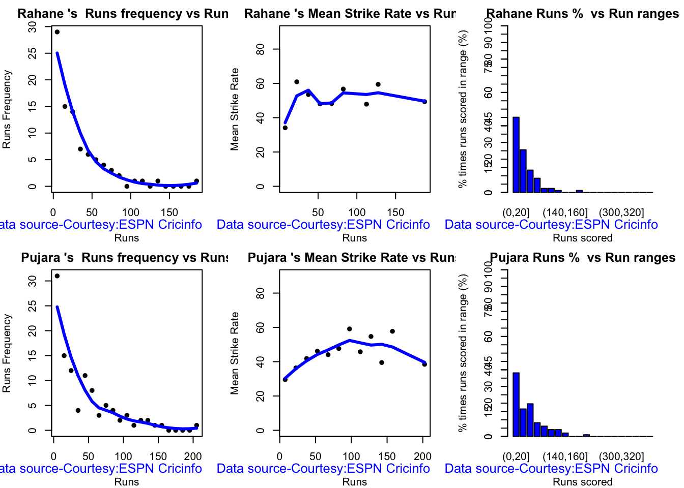
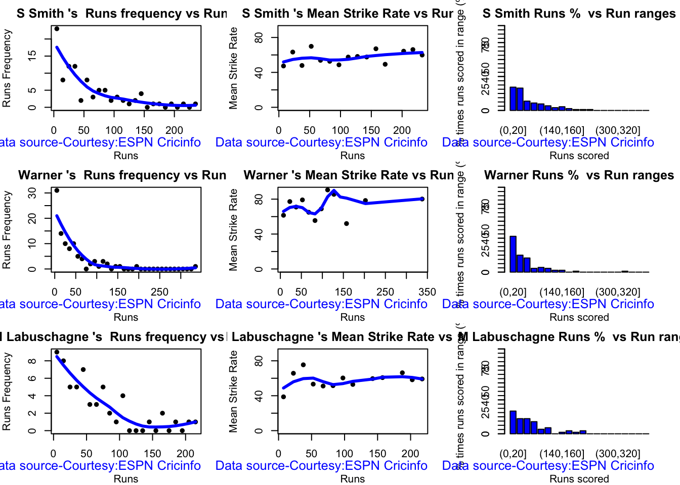
The analyses below include – Runs frequency plot – Mean strike rate – Run Ranges

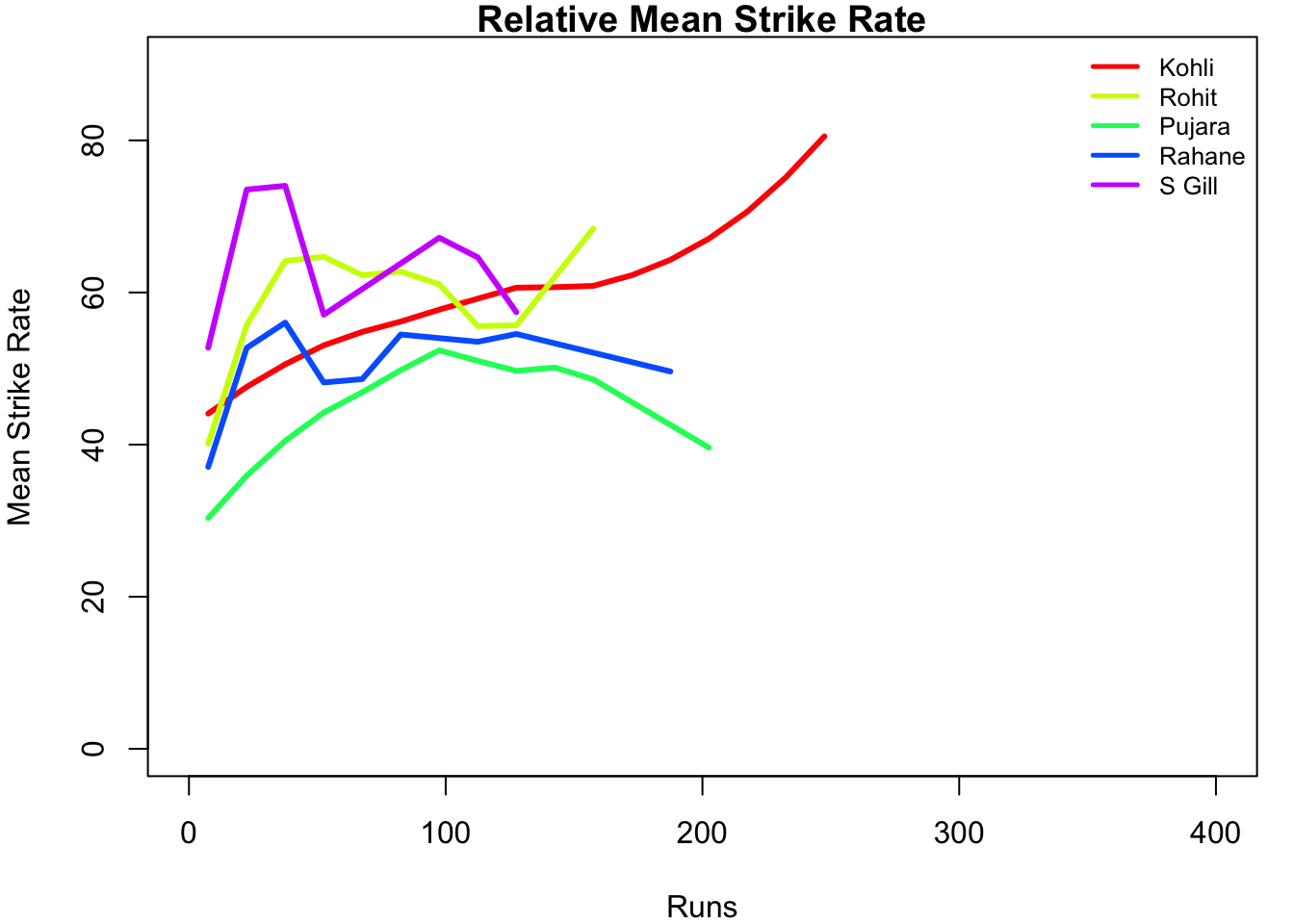
Kohli’s strike rate increases with increasing runs, while Gill’s seems to drop. So it is with Pujara & Rahane

par(mfrow=c(3,3))
par(mar=c(4,4,2,2))
batsmanRunsFreqPerf("kohliTest.csv","Kohli")
batsmanMeanStrikeRate("kohliTest.csv","Kohli")
batsmanRunsRanges("kohliTest.csv","Kohli")

batsmanRunsFreqPerf("rohitTest.csv","Rohit")
batsmanMeanStrikeRate("rohitTest.csv","Rohit")
batsmanRunsRanges("rohitTest.csv","Rohit")

batsmanRunsFreqPerf("shubmanTest.csv","S Gill")
batsmanMeanStrikeRate("shubmanTest.csv","S Gill")
batsmanRunsRanges("shubmanTest.csv","S Gill")

par(mfrow=c(2,3))
par(mar=c(4,4,2,2))
batsmanRunsFreqPerf("rahaneTest.csv","Rahane")
batsmanMeanStrikeRate("rahaneTest.csv","Rahane")
batsmanRunsRanges("rahaneTest.csv","Rahane")

batsmanRunsFreqPerf("pujaraTest.csv","Pujara")
batsmanMeanStrikeRate("pujaraTest.csv","Pujara")
batsmanRunsRanges("pujaraTest.csv","Pujara")

3b. More analyses

Kohli hits roughly 5 4s in his 50 versus Gill,Pujara who is able to smash 6 4s.

par(mfrow=c(3,3))
par(mar=c(4,4,2,2))

batsman4s("kohliTest.csv","Kohli")
batsman6s("kohliTest.csv","Kohli")
batsmanMeanStrikeRate("kohliTest.csv","Kohli")

batsman4s("rohitTest.csv","Rohit")
batsman6s("rohitTest.csv","Rohit")
batsmanMeanStrikeRate("rohitTest.csv","Rohit")

batsman4s("shubmanTest.csv","S Gill")
batsman6s("shubmanTest.csv","S Gill")
batsmanMeanStrikeRate("shubmanTest.csv","S Gill")

par(mfrow=c(2,3))
par(mar=c(4,4,2,2))

batsman4s("rahaneTest.csv","Rahane")
batsman6s("rahaneTest.csv","Rahane")
batsmanMeanStrikeRate("rahane.csv","Rahane")

batsman4s("pujaraTest.csv","Pujara")
batsman6s("pujaraTest.csv","Pujara")
batsmanMeanStrikeRate("pujaraTest.csv","Pujara")

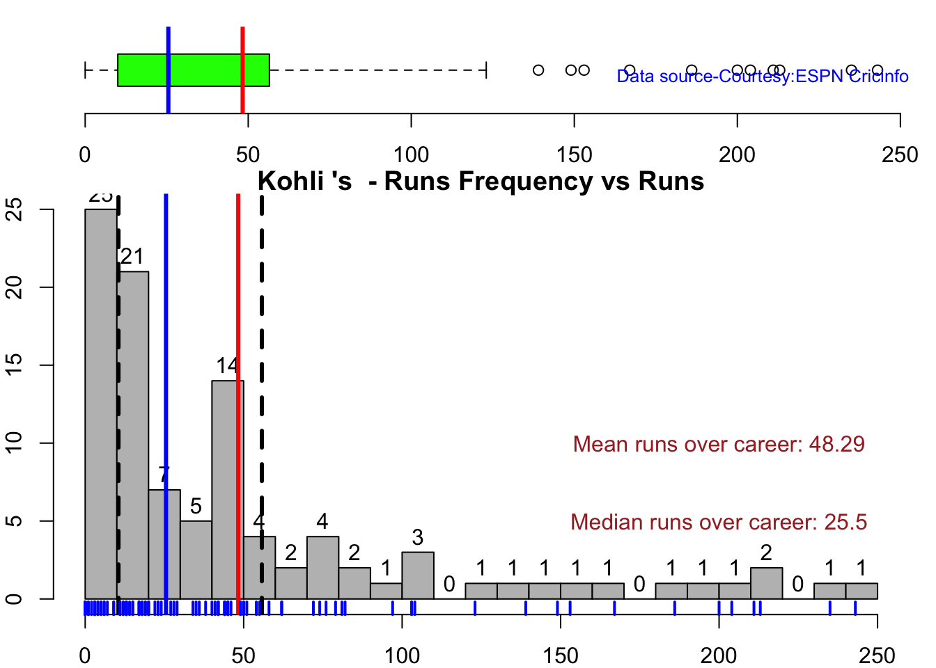
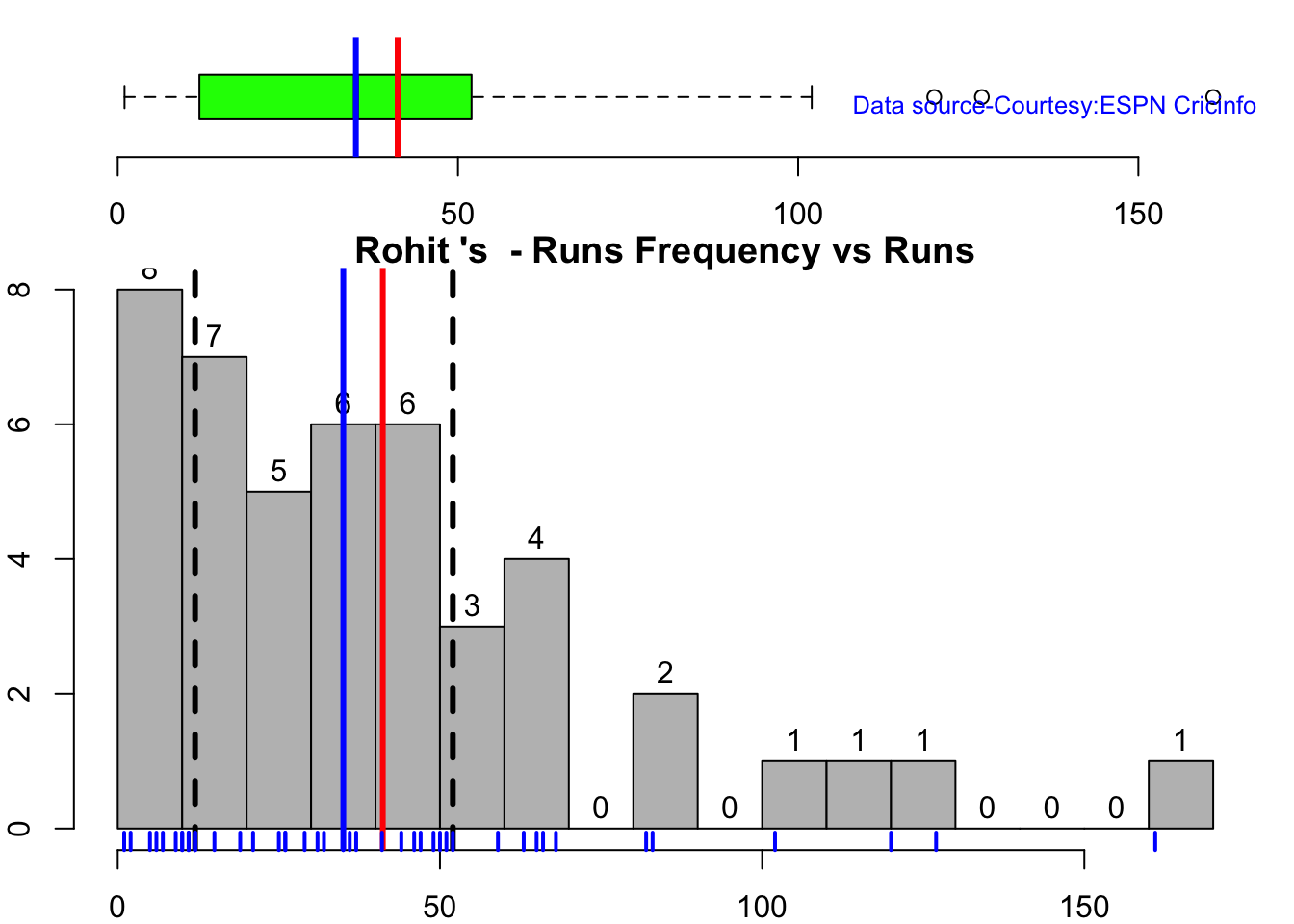
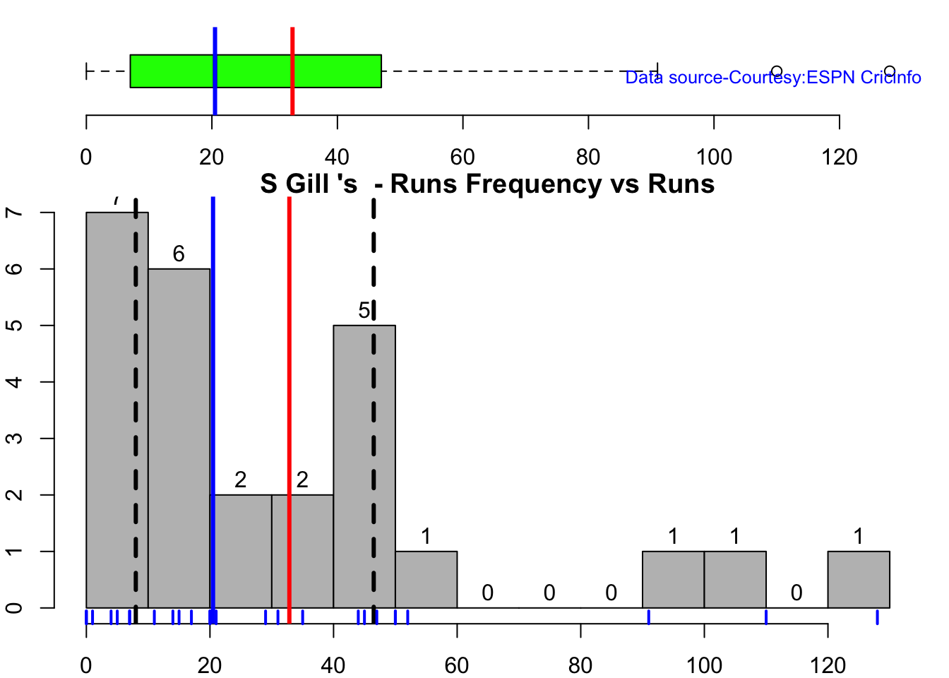
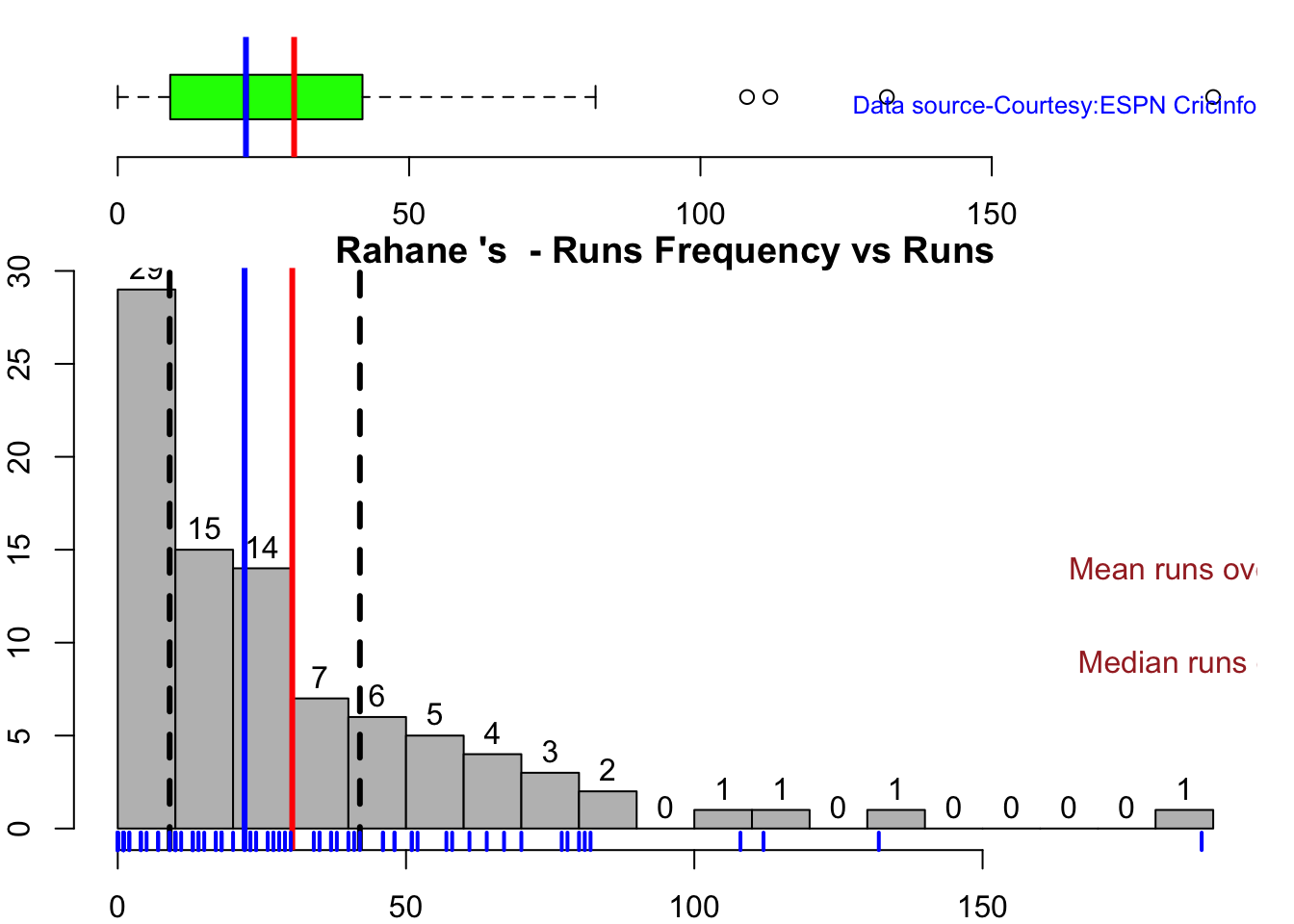
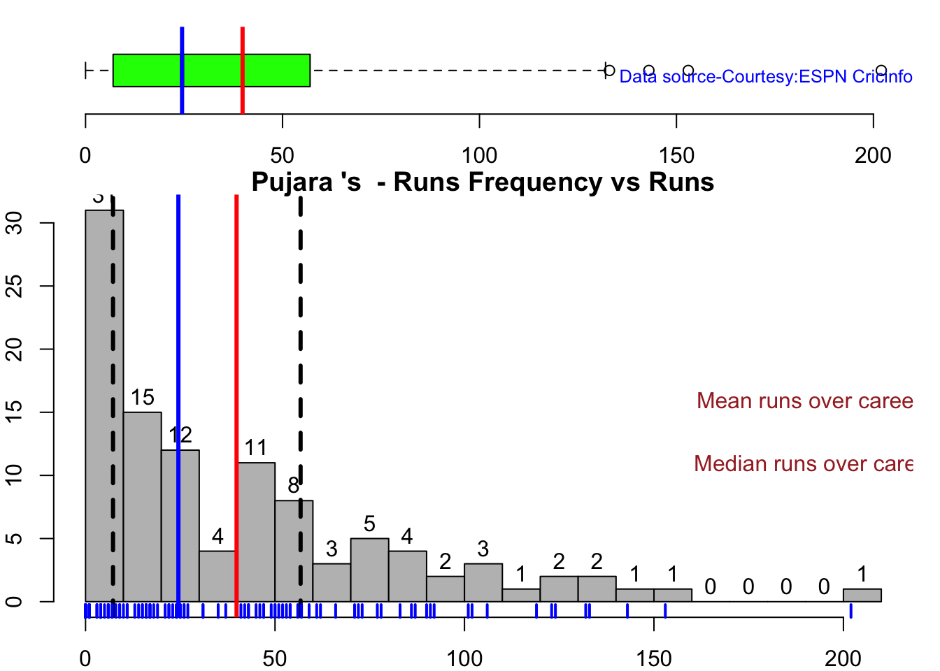
3c.Boxplot histogram plot

This plot shows a combined boxplot of the Runs ranges and a histog2ram of the Runs Frequency Kohli’s average is 48, while Rohit,Pujara is 40 with Rahane and Gill around 33.

batsmanPerfBoxHist("kohliTest.csv","Kohli")

batsmanPerfBoxHist("rohitTest.csv","Rohit")

batsmanPerfBoxHist("shubmanTest.csv","S Gill")

batsmanPerfBoxHist("rahaneTest.csv","Rahane")

batsmanPerfBoxHist("pujaraTest.csv","Pujara")

3d. Contribution to won and lost matches

For the functions below you will have to use the getPlayerDataSp() function. When Rohit Sharma and Pujara have played well India have tended to win more often

par(mfrow=c(2,2))
par(mar=c(4,4,2,2))

batsmanContributionWonLost("kohlisp.csv","Kohli")
batsmanContributionWonLost("rohitsp.csv","Rohit")
batsmanContributionWonLost("rahanesp.csv","Rahane")
batsmanContributionWonLost("pujarasp.csv","Pujara")

3e. Performance at home and overseas

This function also requires the use of getPlayerDataSp() as shown above. This can only be used for Test matches

par(mfrow=c(2,2))
par(mar=c(4,4,2,2))

batsmanPerfHomeAway("kohlisp.csv","Kohli")
batsmanPerfHomeAway("rohitsp.csv","Rohit")
batsmanPerfHomeAway("rahanesp.csv","Rahane")
batsmanPerfHomeAway("pujarasp.csv","Pujara")

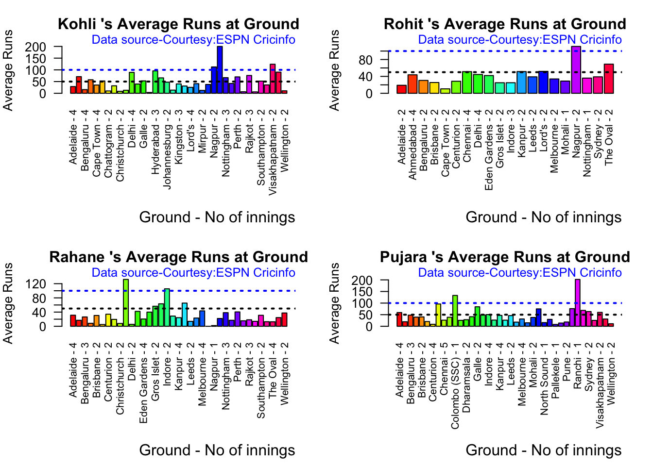
3f. Batsman average at different venues

par(mfrow=c(2,2))
par(mar=c(4,4,2,2))
batsmanAvgRunsGround("kohliTest.csv","Kohli")
batsmanAvgRunsGround("rohitTest.csv","Rohit")
batsmanAvgRunsGround("rahaneTest.csv","Rahane")
batsmanAvgRunsGround("pujaraTest.csv","Pujara")

3g. Batsman average against different opposition

par(mfrow=c(2,2))
par(mar=c(4,4,2,2))
batsmanAvgRunsOpposition("kohliTest.csv","Kohli")
batsmanAvgRunsOpposition("rohitTest.csv","Rohit")
batsmanAvgRunsOpposition("rahaneTest.csv","Rahane")
batsmanAvgRunsOpposition("pujaraTest.csv","Pujara")

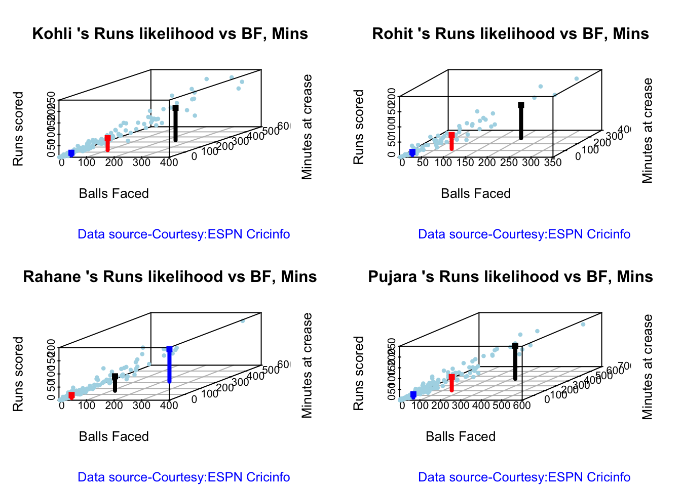
3h. Runs Likelihood of batsman

par(mfrow=c(2,2))
par(mar=c(4,4,2,2))
batsmanRunsLikelihood("kohli.csv","Kohli")

## Summary of  Kohli 's runs scoring likelihood
## **************************************************
## 
## There is a 52.91 % likelihood that Kohli  will make  12 Runs in  26 balls over 35  Minutes 
## There is a 30.81 % likelihood that Kohli  will make  52 Runs in  100 balls over  139  Minutes 
## There is a 16.28 % likelihood that Kohli  will make  142 Runs in  237 balls over 335  Minutes

batsmanRunsLikelihood("rohit.csv","Rohit")

## Summary of  Rohit 's runs scoring likelihood
## **************************************************
## 
## There is a 43.24 % likelihood that Rohit  will make  10 Runs in  21 balls over 32  Minutes 
## There is a 45.95 % likelihood that Rohit  will make  46 Runs in  85 balls over  124  Minutes 
## There is a 10.81 % likelihood that Rohit  will make  110 Runs in  199 balls over 282  Minutes

batsmanRunsLikelihood("rahane.csv","Rahane")

## Summary of  Rahane 's runs scoring likelihood
## **************************************************
## 
## There is a 7.75 % likelihood that Rahane  will make  124 Runs in  224 balls over 318  Minutes 
## There is a 62.02 % likelihood that Rahane  will make  12 Runs in  26 balls over  37  Minutes 
## There is a 30.23 % likelihood that Rahane  will make  55 Runs in  113 balls over 162  Minutes

batsmanRunsLikelihood("pujara.csv","Pujara")

## Summary of  Pujara 's runs scoring likelihood
## **************************************************
## 
## There is a 60.49 % likelihood that Pujara  will make  15 Runs in  38 balls over 55  Minutes 
## There is a 31.48 % likelihood that Pujara  will make  62 Runs in  142 balls over  204  Minutes 
## There is a 8.02 % likelihood that Pujara  will make  153 Runs in  319 balls over 445  Minutes

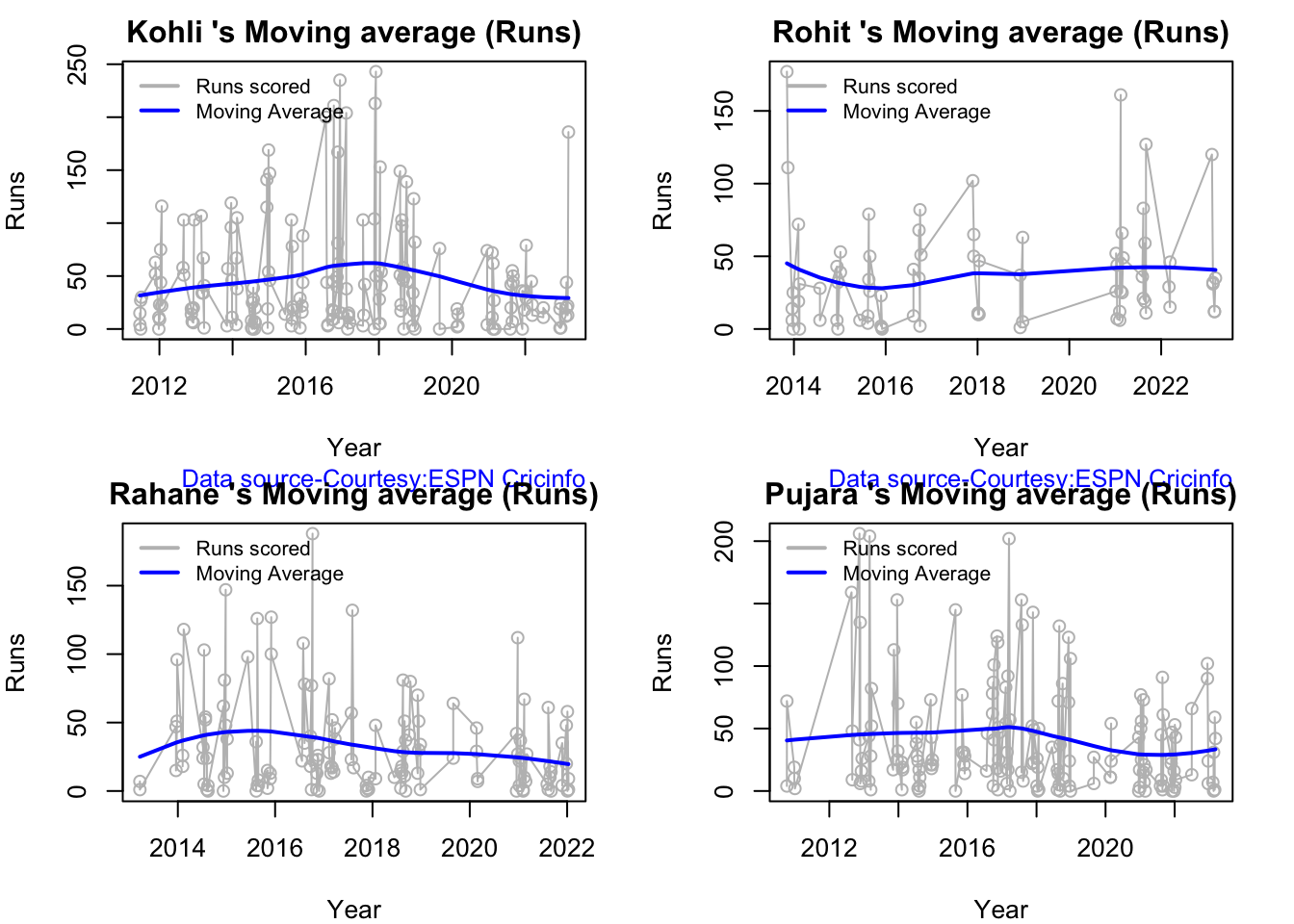
3h1. Moving average of batsman

Kohli’s moving average in tests seem to havw dropped after a peak in 2017, 2018. So it is with Rahane

par(mfrow=c(2,2))
par(mar=c(4,4,2,2))
batsmanMovingAverage("kohli.csv","Kohli")
batsmanMovingAverage("rohit.csv","Rohit")
batsmanMovingAverage("rahane.csv","Rahane")
batsmanMovingAverage("pujara.csv","Pujara")

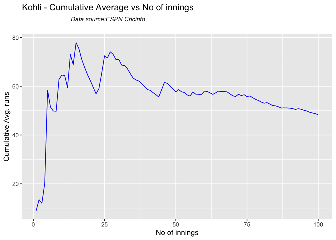
3i. Cumulative Average runs of batsman in career

Kohli’s cumulative average averages to ~48. Shubman Gill’s cumulative average is on the rise.

par(mfrow=c(2,2))
par(mar=c(4,4,2,2))
batsmanCumulativeAverageRuns("kohliTest.csv","Kohli")

batsmanCumulativeAverageRuns("rohitTest.csv","Rohit")

batsmanCumulativeAverageRuns("rahaneTest.csv","Rahane")

batsmanCumulativeAverageRuns("pujaraTest.csv","Pujara")

batsmanCumulativeAverageRuns("shubmanTest.csv","S Gill")

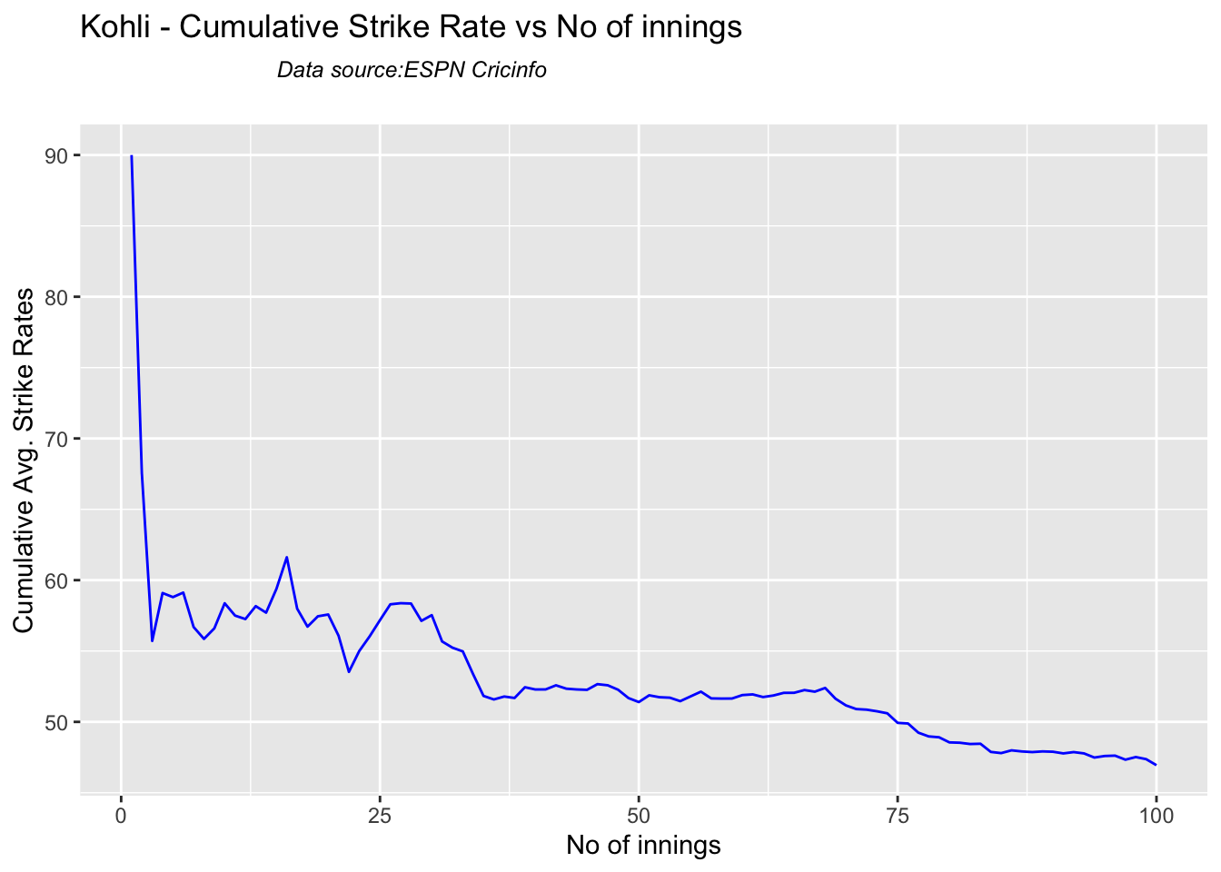
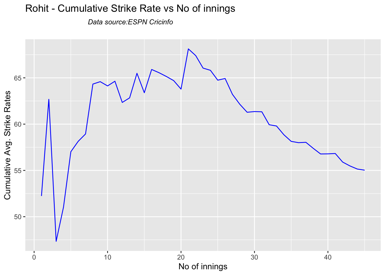
3j Cumulative Average strike rate of batsman in career

par(mfrow=c(2,2))
par(mar=c(4,4,2,2))

batsmanCumulativeStrikeRate("kohliTest.csv","Kohli")

batsmanCumulativeStrikeRate("rohitTest.csv","Rohit")

batsmanCumulativeStrikeRate("rahaneTest.csv","Rahane")

batsmanCumulativeStrikeRate("pujaraTest.csv","Pujara")

batsmanCumulativeStrikeRate("shubmanTest.csv","S Gill")

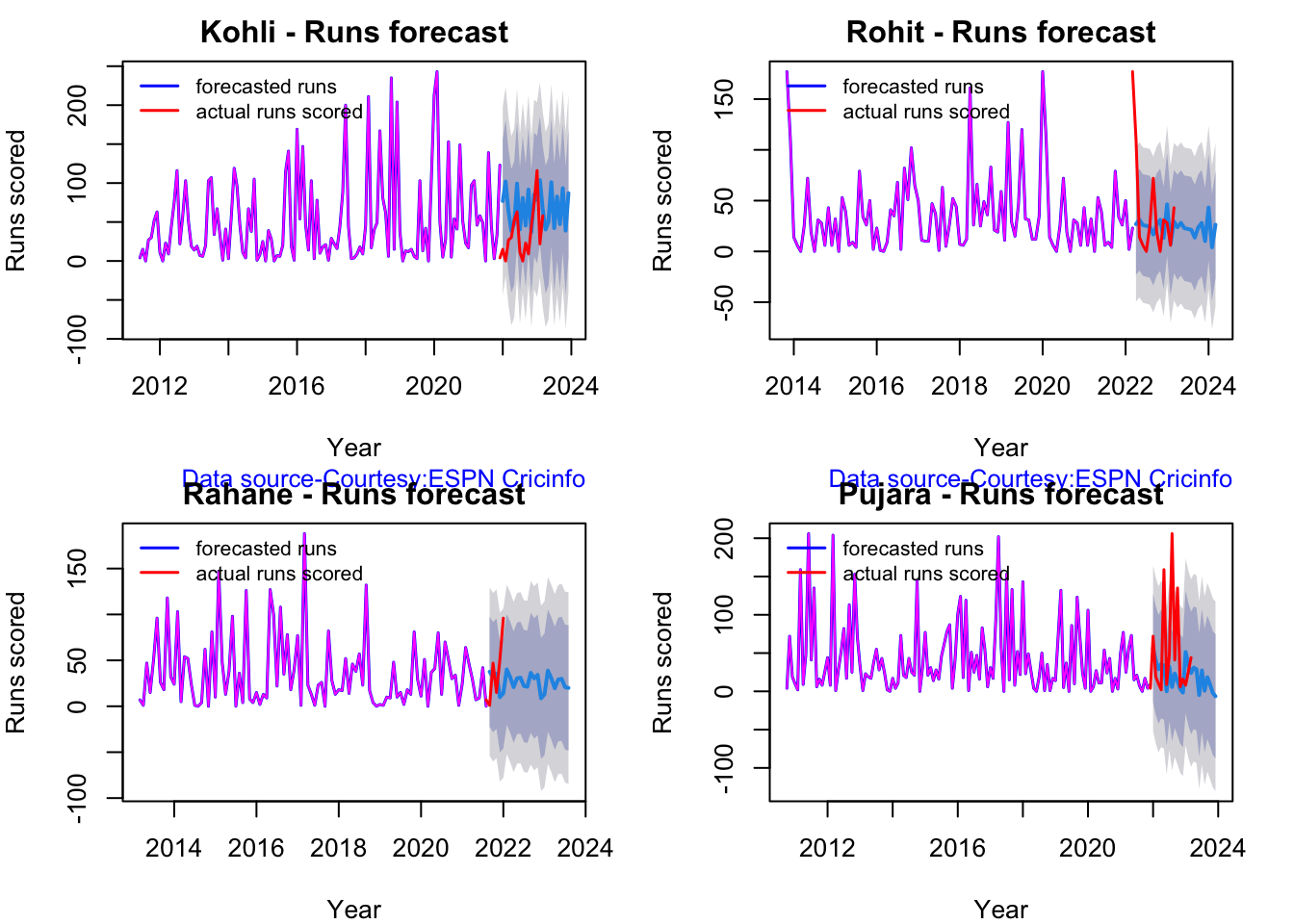
3k. Future Runs forecast

Here are plots that forecast how the batsman will perform in future. In this case 90% of the career runs trend is uses as the training set. the remaining 10% is the test set.

A Holt-Winters forecating model is used to forecast future performance based on the 90% training set. The forecated runs trend is plotted. The test set is also plotted to see how close the forecast and the actual matches

Take a look at the runs forecasted for the batsman below.

par(mfrow=c(2,2))
par(mar=c(4,4,2,2))

batsmanPerfForecast("kohli.csv","Kohli")
batsmanPerfForecast("rohit.csv","Rohit")
batsmanPerfForecast("rahane.csv","Rahane")
batsmanPerfForecast("pujara.csv","Pujara")

3l. Relative Mean Strike Rate plot

The plot below compares the Mean Strike Rate of the batsman for each of the runs ranges of 10 and plots them. The plot indicate the following

frames <- list("kohliTest.csv","rohitTest.csv","pujaraTest.csv","rahaneTest.csv","shubmanTest.csv")
names <- list("Kohli","Rohit","Pujara","Rahane","S Gill")
relativeBatsmanSR(frames,names)

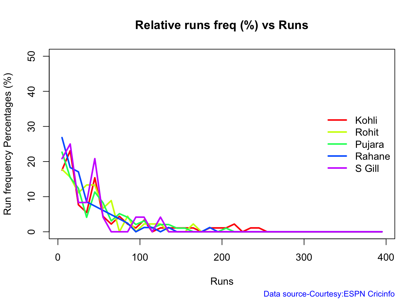
3m. Relative Runs Frequency plot

The plot below gives the relative Runs Frequency Percetages for each 10 run bucket. The plot below show

frames <- list("kohliTest.csv","rohitTest.csv","pujaraTest.csv","rahaneTest.csv","shubmanTest.csv")
names <- list("Kohli","Rohit","Pujara","Rahane","S Gill")
relativeRunsFreqPerf(frames,names)

3n. Relative cumulative average runs in career

Kohli’s tops the list, followed by Pujara and Rohit is 3rd. Gill is on the upswing. Hope he performs well.

frames <- list("kohliTest.csv","rohitTest.csv","pujaraTest.csv","rahaneTest.csv","shubmanTest.csv")
names <- list("Kohli","Rohit","Pujara","Rahane","S Gill")
relativeBatsmanCumulativeAvgRuns(frames,names)

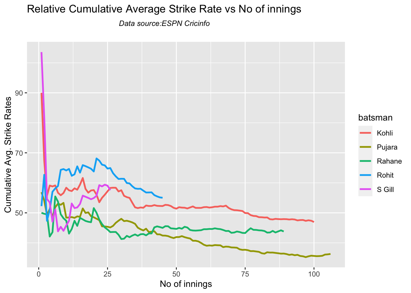
3o. Relative cumulative average strike rate in career

ROhit has the best strike rate followed by Kohli, with Shubman Gill ctaching up fast

frames <- list("kohliTest.csv","rohitTest.csv","pujaraTest.csv","rahaneTest.csv","shubmanTest.csv")
names <- list("Kohli","Rohit","Pujara","Rahane","S Gill")
relativeBatsmanCumulativeStrikeRate(frames,names)

3p. Check Batsman In-Form or Out-of-Form

The below computation uses Null Hypothesis testing and p-value to determine if the batsman is in-form or out-of-form. For this 90% of the career runs is chosen as the population and the mean computed. The last 10% is chosen to be the sample set and the sample Mean and the sample Standard Deviation are caculated.

The Null Hypothesis (H0) assumes that the batsman continues to stay in-form where the sample mean is within 95% confidence interval of population mean The Alternative (Ha) assumes that the batsman is out of form the sample mean is beyond the 95% confidence interval of the population mean.

A significance value of 0.05 is chosen and p-value us computed If p-value >= .05 – Batsman In-Form If p-value < 0.05 – Batsman Out-of-Form

Note Ideally the p-value should be done for a population that follows the Normal Distribution. But the runs population is usually left skewed. So some correction may be needed. I will revisit this later

This is done for the Top 4 batsman

checkBatsmanInForm("kohli.csv","Kohli")

## [1] "**************************** Form status of Kohli ****************************\n\n Population size: 154  Mean of population: 47.03 \n Sample size: 18  Mean of sample: 32.22 SD of sample: 42.45 \n\n Null hypothesis H0 : Kohli 's sample average is within 95% confidence interval of population average\n Alternative hypothesis Ha : Kohli 's sample average is below the 95% confidence interval of population average\n\n Kohli 's Form Status: In-Form because the p value: 0.078058  is greater than alpha=  0.05 \n *******************************************************************************************\n\n"

checkBatsmanInForm("rohit.csv","Rohit")

## [1] "**************************** Form status of Rohit ****************************\n\n Population size: 66  Mean of population: 37.03 \n Sample size: 8  Mean of sample: 37.88 SD of sample: 35.38 \n\n Null hypothesis H0 : Rohit 's sample average is within 95% confidence interval of population average\n Alternative hypothesis Ha : Rohit 's sample average is below the 95% confidence interval of population average\n\n Rohit 's Form Status: In-Form because the p value: 0.526254  is greater than alpha=  0.05 \n *******************************************************************************************\n\n"

checkBatsmanInForm("rahane.csv","Rahane")

## [1] "**************************** Form status of Rahane ****************************\n\n Population size: 116  Mean of population: 34.78 \n Sample size: 13  Mean of sample: 21.38 SD of sample: 21.96 \n\n Null hypothesis H0 : Rahane 's sample average is within 95% confidence interval of population average\n Alternative hypothesis Ha : Rahane 's sample average is below the 95% confidence interval of population average\n\n Rahane 's Form Status: Out-of-Form because the p value: 0.023244  is less than alpha=  0.05 \n *******************************************************************************************\n\n"

checkBatsmanInForm("pujara.csv","Pujara")

## [1] "**************************** Form status of Pujara ****************************\n\n Population size: 145  Mean of population: 41.93 \n Sample size: 17  Mean of sample: 33.24 SD of sample: 31.74 \n\n Null hypothesis H0 : Pujara 's sample average is within 95% confidence interval of population average\n Alternative hypothesis Ha : Pujara 's sample average is below the 95% confidence interval of population average\n\n Pujara 's Form Status: In-Form because the p value: 0.137319  is greater than alpha=  0.05 \n *******************************************************************************************\n\n"

checkBatsmanInForm("shubman.csv","S Gill")

## [1] "**************************** Form status of S Gill ****************************\n\n Population size: 23  Mean of population: 30.43 \n Sample size: 3  Mean of sample: 51.33 SD of sample: 66.88 \n\n Null hypothesis H0 : S Gill 's sample average is within 95% confidence interval of population average\n Alternative hypothesis Ha : S Gill 's sample average is below the 95% confidence interval of population average\n\n S Gill 's Form Status: In-Form because the p value: 0.687033  is greater than alpha=  0.05 \n *******************************************************************************************\n\n"

3q. Predicting Runs given Balls Faced and Minutes at Crease

A multi-variate regression plane is fitted between Runs and Balls faced +Minutes at crease.

BF <- seq( 10, 400,length=15)
Mins <- seq(30,600,length=15)
newDF <- data.frame(BF,Mins)
kohli1 <- batsmanRunsPredict("kohli.csv","Kohli",newdataframe=newDF)
rohit1 <- batsmanRunsPredict("rohit.csv","Rohit",newdataframe=newDF)
pujara1 <- batsmanRunsPredict("pujara.csv","Pujara",newdataframe=newDF)
rahane1 <- batsmanRunsPredict("rahane.csv","Rahane",newdataframe=newDF)
sgill1 <- batsmanRunsPredict("shubman.csv","S Gill",newdataframe=newDF)

batsmen <-cbind(round(kohli1$Runs),round(rohit1$Runs),round(pujara1$Runs),round(rahane1$Runs),round(sgill1$Runs))
colnames(batsmen) <- c("Kohli","Rohit","Pujara","Rahane","S Gill")
newDF <- data.frame(round(newDF$BF),round(newDF$Mins))
colnames(newDF) <- c("BallsFaced","MinsAtCrease")
predictedRuns <- cbind(newDF,batsmen)
predictedRuns

##    BallsFaced MinsAtCrease Kohli Rohit Pujara Rahane S Gill
## 1          10           30     6     3      3      2      7
## 2          38           71    24    19     16     17     24
## 3          66          111    41    35     29     31     40
## 4          94          152    58    51     42     45     56
## 5         121          193    76    66     55     59     73
## 6         149          234    93    82     68     74     89
## 7         177          274   110    98     80     88    106
## 8         205          315   128   114     93    102    122
## 9         233          356   145   129    106    116    139
## 10        261          396   163   145    119    130    155
## 11        289          437   180   161    132    145    171
## 12        316          478   197   177    144    159    188
## 13        344          519   215   192    157    173    204
## 14        372          559   232   208    170    187    221
## 15        400          600   249   224    183    202    237

4. Analysis of India WTC batsmen from Jan 2016 – May 2023 against Australia

4a. Relative cumulative average

Against Australia specifically between 2016 – 2023, Pujara has the best record followed by Rahane, with Gill in hot pursuit. Kohli and Rohit trail behind

frames <- list("kohliTestAus.csv","rohitTestAus.csv","pujaraTestAus.csv","rahaneTestAus.csv","shubmanTestAus.csv")
names <- list("Kohli","Rohit","Pujara","Rahane","S Gill")
relativeBatsmanCumulativeAvgRuns(frames,names)

4b. Relative cumulative average strike rate in career

In the Strike Rate department Gill tops followed by Rohit and Rahane

frames <- list("kohliTestAus.csv","rohitTestAus.csv","pujaraTestAus.csv","rahaneTestAus.csv","shubmanTestAus.csv")
names <- list("Kohli","Rohit","Pujara","Rahane","S Gill")
relativeBatsmanCumulativeStrikeRate(frames,names)

5. Analysis of Australia WTC batsmen from Jan 2016 – May 2023

5a Basic analyses

par(mfrow=c(3,3))
par(mar=c(4,4,2,2))
batsmanRunsFreqPerf("stevesmithTest.csv","S Smith")
batsmanMeanStrikeRate("stevesmithTest.csv","S Smith")
batsmanRunsRanges("stevesmithTest.csv","S Smith")

batsmanRunsFreqPerf("warnerTest.csv","Warner")
batsmanMeanStrikeRate("warnerTest.csv","Warner")
batsmanRunsRanges("warnerTest.csv","Warner")

batsmanRunsFreqPerf("labuschagneTest.csv","M Labuschagne")
batsmanMeanStrikeRate("labuschagneTest.csv","M Labuschagne")
batsmanRunsRanges("labuschagneTest.csv","M Labuschagne")

par(mfrow=c(2,3))
par(mar=c(4,4,2,2))
batsmanRunsFreqPerf("cgreenTest.csv","C Green")
batsmanMeanStrikeRate("cgreenTest.csv","C Green")
batsmanRunsRanges("cgreenTest.csv","C Green")

batsmanRunsFreqPerf("khwajaTest.csv","Khwaja")
batsmanMeanStrikeRate("khwajaTest.csv","Khwaja")
batsmanRunsRanges("khwajaTest.csv","Khwaja")

5b. More analyses

par(mfrow=c(3,3))
par(mar=c(4,4,2,2))
batsman4s("stevesmithTest.csv","S Smith")
batsman6s("stevesmithTest.csv","S Smith")
batsmanMeanStrikeRate("stevesmithTest.csv","S Smith")

batsman4s("warnerTest.csv","Warner")
batsman6s("warnerTest.csv","Warner")
batsmanMeanStrikeRate("warnerTest.csv","Warner")

batsman4s("labuschagneTest.csv","M Labuschagne")
batsman6s("labuschagneTest.csv","M Labuschagne")
batsmanMeanStrikeRate("labuschagneTest.csv","M Labuschagne")

par(mfrow=c(2,3))
par(mar=c(4,4,2,2))
batsman4s("cgreenTest.csv","C Green")
batsman6s("cgreenTest.csv","C Green")
batsmanMeanStrikeRate("cgreenTest.csv","C Green")

batsman4s("khwajaTest.csv","Khwaja")
batsman6s("khwajaTest.csv","Khwaja")
batsmanMeanStrikeRate("khwajaTest.csv","Khwaja")

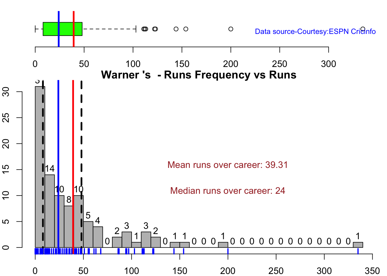
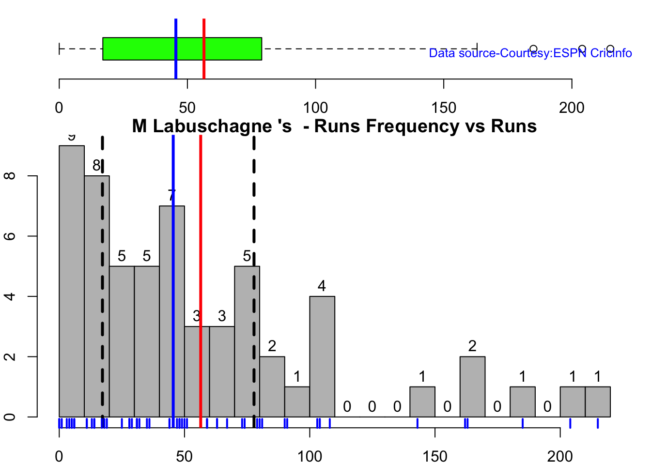
5c.Boxplot histogram plot

This plot shows a combined boxplot of the Runs ranges and a histog2ram of the Runs Frequency

Smith, Labuschagne has an average of 53+ since 2016!! Warner & Khwaja are at ~46

batsmanPerfBoxHist("stevesmithTest.csv","S Smith")

batsmanPerfBoxHist("warnerTest.csv","Warner")

batsmanPerfBoxHist("labuschagneTest.csv","M Labuschagne")

batsmanPerfBoxHist("cgreenTest.csv","C Green")

batsmanPerfBoxHist("khwajaTest.csv","Khwaja")

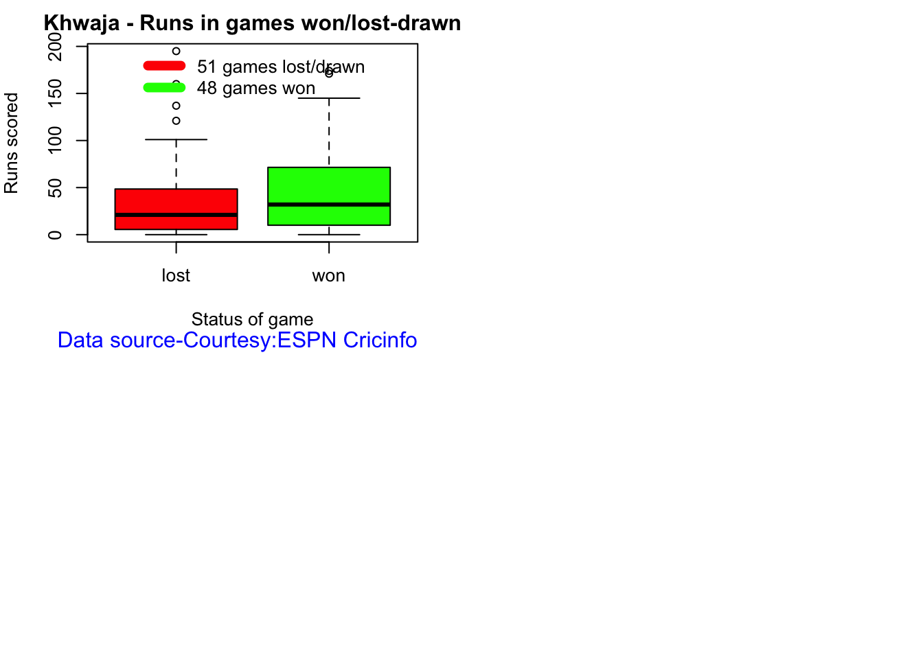
5d. Contribution to won and lost matches

For the 2 functions below you will have to use the getPlayerDataSp() function. Australia has won matches when Smith, Warner and Khwaja have played well.

par(mfrow=c(2,2))
par(mar=c(4,4,2,2))
batsmanContributionWonLost("stevesmithsp.csv","S Smith")
batsmanContributionWonLost("warnersp.csv","Warner")
batsmanContributionWonLost("labuschagnesp.csv","M Labuschagne")
batsmanContributionWonLost("cgreensp.csv","C Green")

batsmanContributionWonLost("khwajasp.csv","Khwaja")

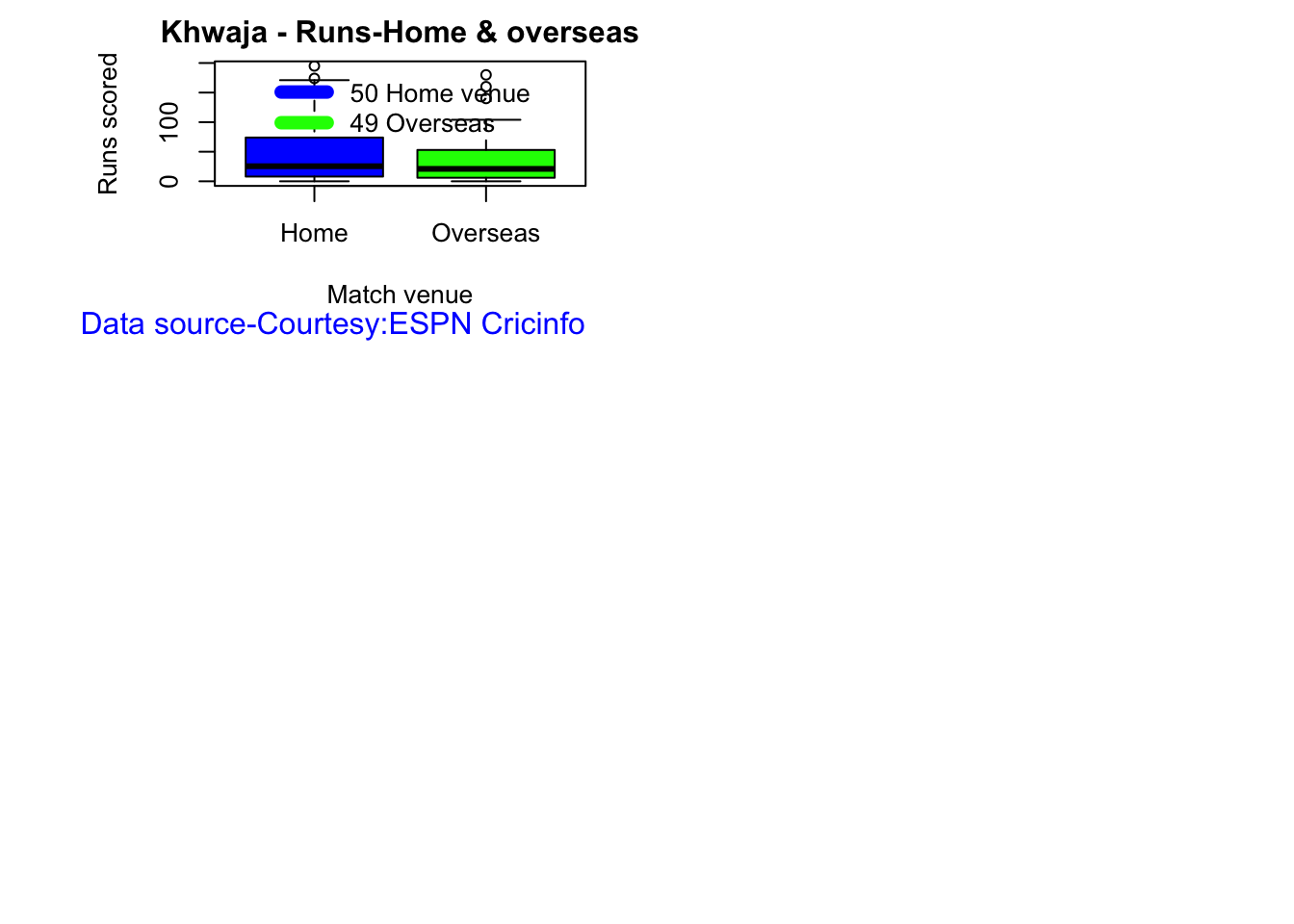
5e. Performance at home and overseas

This function also requires the use of getPlayerDataSp() as shown above. This can only be used for Test matches

par(mfrow=c(2,2))
par(mar=c(4,4,2,2))

batsmanPerfHomeAway("stevesmithsp.csv","S Smith")
batsmanPerfHomeAway("warnersp.csv","Warner")
batsmanPerfHomeAway("labuschagnesp.csv","M Labuschagne")
batsmanPerfHomeAway("cgreensp.csv","C Green")

batsmanPerfHomeAway("khwajasp.csv","Khwaja")

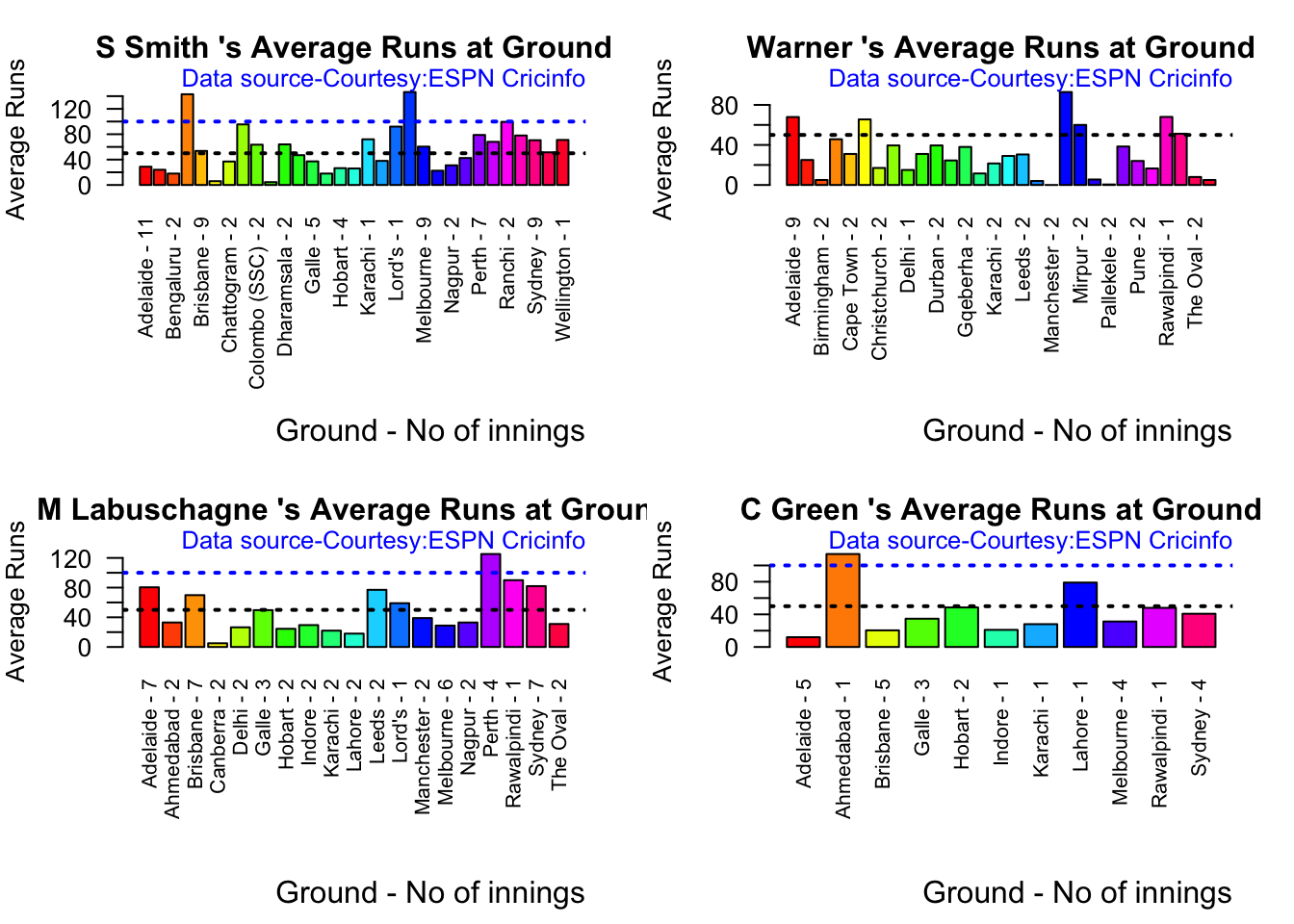
5f. Batsman average at different venues

par(mfrow=c(2,2))
par(mar=c(4,4,2,2))

batsmanAvgRunsGround("stevesmithTest.csv","S Smith")
batsmanAvgRunsGround("warnerTest.csv","Warner")
batsmanAvgRunsGround("labuschagneTest.csv","M Labuschagne")
batsmanAvgRunsGround("cgreenTest.csv","C Green")

batsmanAvgRunsGround("khwajaTest.csv","Khwaja")

5g. Batsman average against different opposition

par(mfrow=c(2,2))
par(mar=c(4,4,2,2))

batsmanAvgRunsOpposition("stevesmithTest.csv","S Smith")
batsmanAvgRunsOpposition("warnerTest.csv","Warner")
batsmanAvgRunsOpposition("labuschagneTest.csv","M Labuschagne")
batsmanAvgRunsOpposition("khwajaTest.csv","Khwaja")

5h. Runs Likelihood of batsman

par(mfrow=c(2,2))
par(mar=c(4,4,2,2))

batsmanRunsLikelihood("stevesmithTest.csv","S Smith")

## Summary of  S Smith 's runs scoring likelihood
## **************************************************
## 
## There is a 58.76 % likelihood that S Smith  will make  21 Runs in  38 balls over 56  Minutes 
## There is a 24.74 % likelihood that S Smith  will make  70 Runs in  148 balls over  210  Minutes 
## There is a 16.49 % likelihood that S Smith  will make  148 Runs in  268 balls over 398  Minutes

batsmanRunsLikelihood("warnerTest.csv","Warner")

## Summary of  Warner 's runs scoring likelihood
## **************************************************
## 
## There is a 7.22 % likelihood that Warner  will make  155 Runs in  253 balls over 372  Minutes 
## There is a 62.89 % likelihood that Warner  will make  14 Runs in  21 balls over  32  Minutes 
## There is a 29.9 % likelihood that Warner  will make  65 Runs in  94 balls over 135  Minutes

batsmanRunsLikelihood("labuschagneTest.csv","M Labuschagne")

## Summary of  M Labuschagne 's runs scoring likelihood
## **************************************************
## 
## There is a 32.76 % likelihood that M Labuschagne  will make  74 Runs in  144 balls over 206  Minutes 
## There is a 55.17 % likelihood that M Labuschagne  will make  22 Runs in  37 balls over  54  Minutes 
## There is a 12.07 % likelihood that M Labuschagne  will make  168 Runs in  297 balls over 420  Minutes

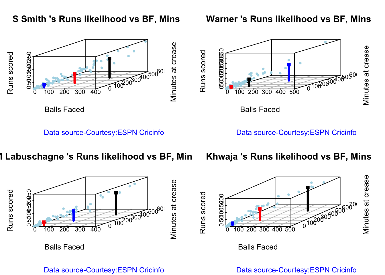
batsmanRunsLikelihood("khwajaTest.csv","Khwaja")

## Summary of  Khwaja 's runs scoring likelihood
## **************************************************
## 
## There is a 64.94 % likelihood that Khwaja  will make  14 Runs in  29 balls over 42  Minutes 
## There is a 27.27 % likelihood that Khwaja  will make  79 Runs in  148 balls over  210  Minutes 
## There is a 7.79 % likelihood that Khwaja  will make  165 Runs in  351 balls over 515  Minutes

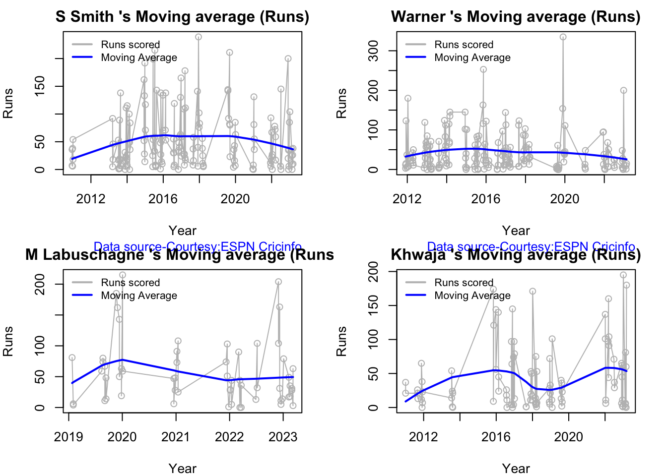
5i. Moving average of batsman

Smith and Warner’s moving average has been on a downward trend lately. Khwaja is playing well

par(mfrow=c(2,2))
par(mar=c(4,4,2,2))

batsmanMovingAverage("stevesmith.csv","S Smith")
batsmanMovingAverage("warner.csv","Warner")
batsmanMovingAverage("labuschagne.csv","M Labuschagne")
batsmanMovingAverage("khwaja.csv","Khwaja")

5j. Cumulative Average runs of batsman in career

Labuschagne, SMith and Warner havwe very good cumulative average

par(mfrow=c(2,2))
par(mar=c(4,4,2,2))

batsmanCumulativeAverageRuns("stevesmithTest.csv","S Smith")

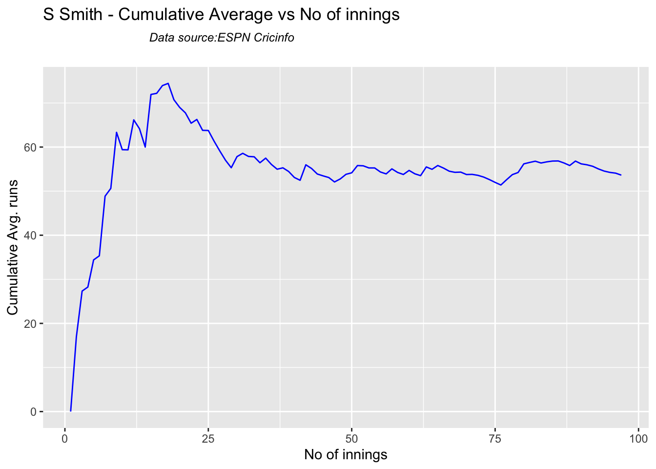
batsmanCumulativeAverageRuns("warnerTest.csv","Warner")

batsmanCumulativeAverageRuns("labuschagneTest.csv","M Labuschagne")

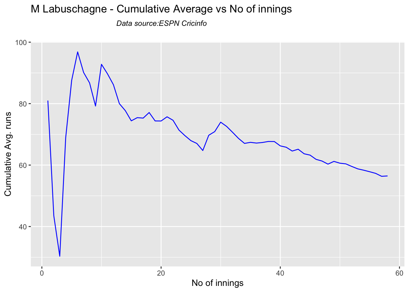
batsmanCumulativeAverageRuns("khwajaTest.csv","Khwaja")

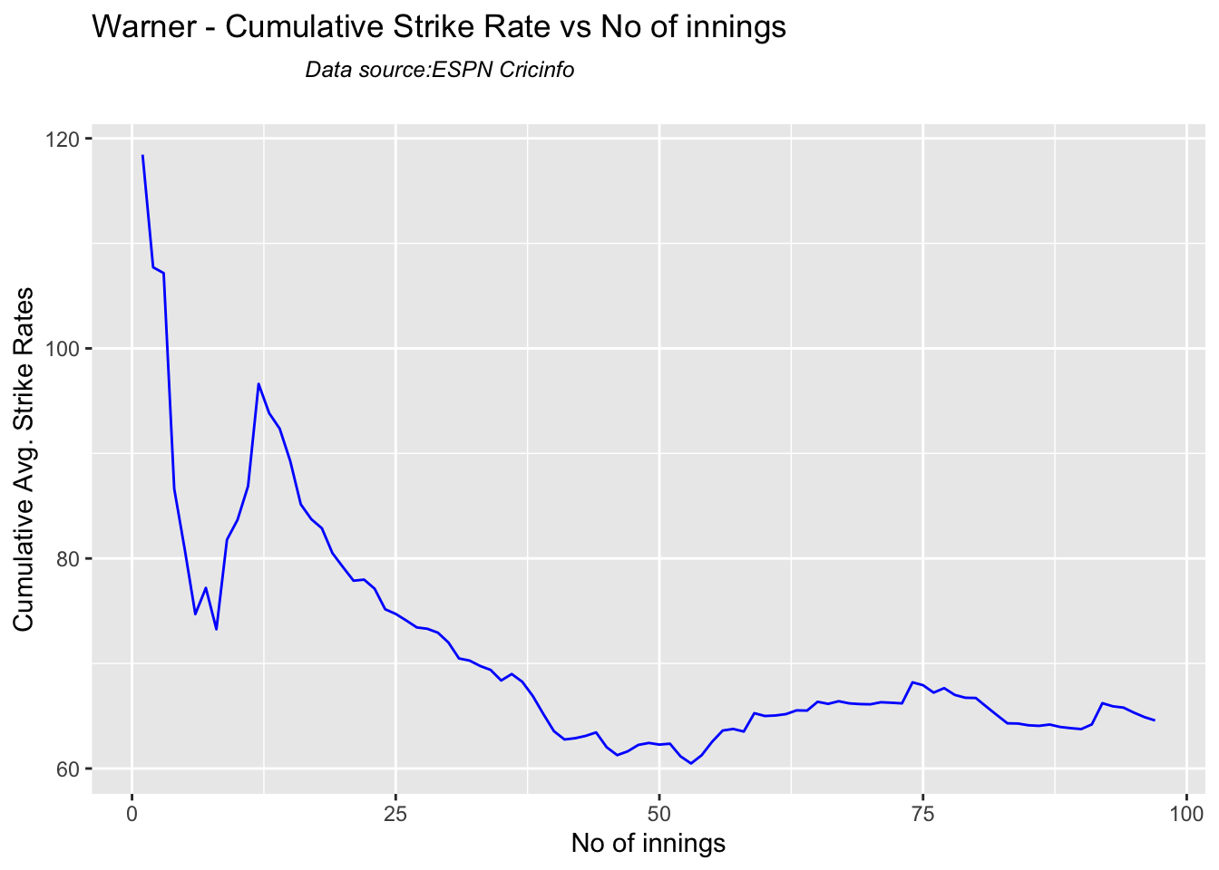
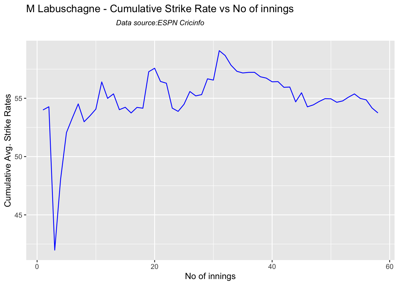
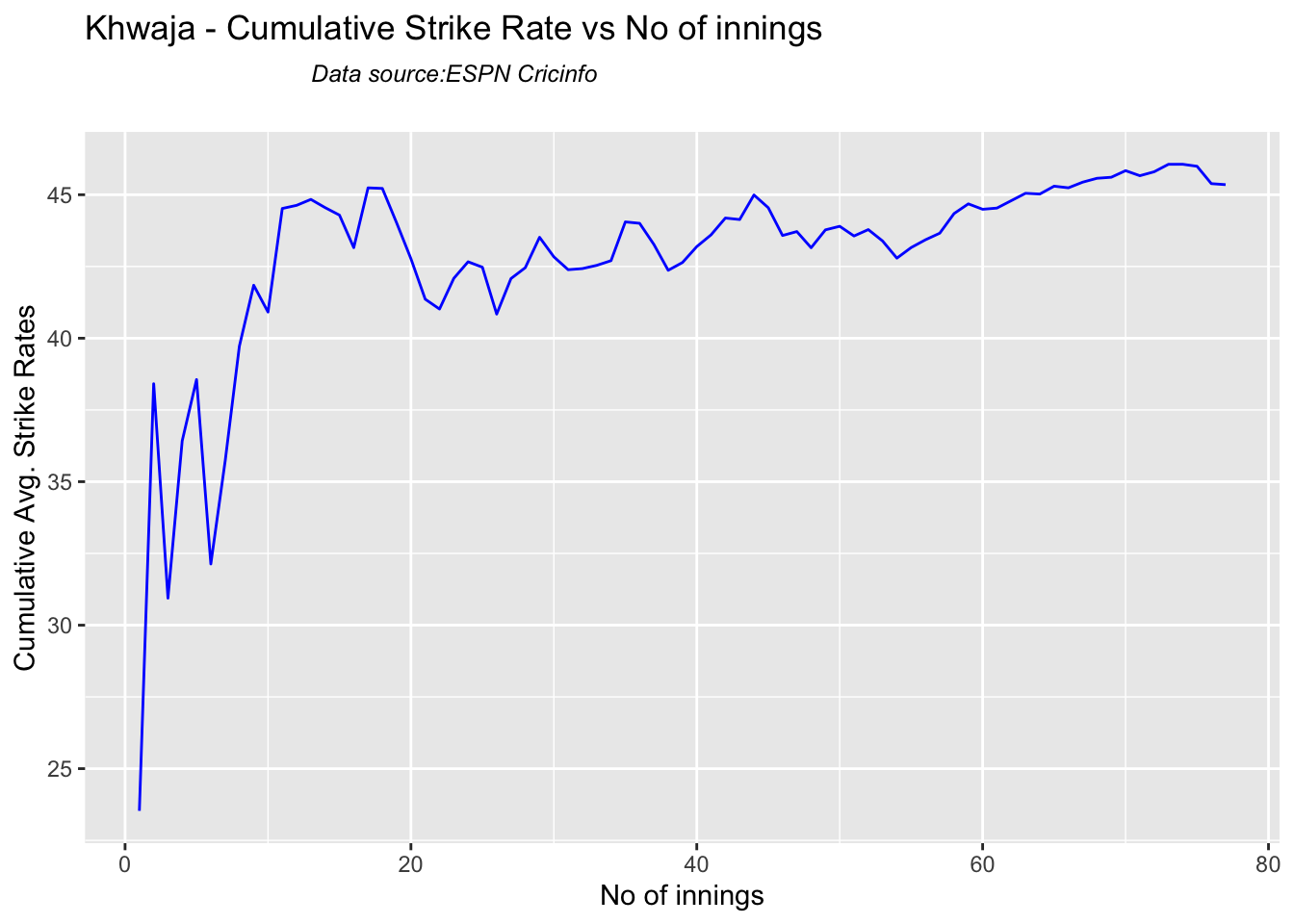
5k. Cumulative Average strike rate of batsman in career

Warner towers over the others in the cumulative strike rate, followed by Labuschagne and Smith

par(mfrow=c(2,2))
par(mar=c(4,4,2,2))

batsmanCumulativeStrikeRate("stevesmithTest.csv","S Smith")

batsmanCumulativeStrikeRate("warnerTest.csv","Warner")

batsmanCumulativeStrikeRate("labuschagneTest.csv","M Labuschagne")

batsmanCumulativeStrikeRate("khwajaTest.csv","Khwaja")

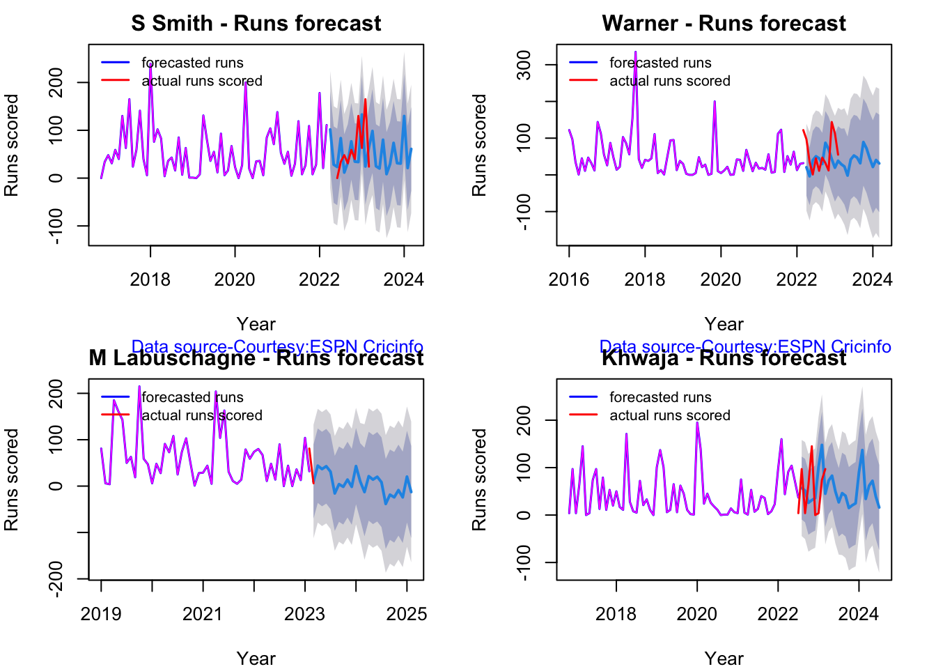
5l. Future Runs forecast

Here are plots that forecast how the batsman will perform in future. In this case 90% of the career runs trend is uses as the training set. the remaining 10% is the test set.

Take a look at the runs forecasted for the batsman below.

par(mfrow=c(2,2))
par(mar=c(4,4,2,2))

batsmanPerfForecast("stevesmithTest.csv","S Smith")
batsmanPerfForecast("warnerTest.csv","Warner")
batsmanPerfForecast("labuschagneTest.csv","M Labuschagne")
batsmanPerfForecast("khwajaTest.csv","Khwaja")

5m. Relative Mean Strike Rate plot

The plot below compares the Mean Strike Rate of the batsman for each of the runs ranges of 10 and plots them. The plot indicate the following

frames <- list("stevesmithTest.csv","warnerTest.csv","khwajaTest.csv","labuschagneTest.csv","cgreenTest.csv")
names <- list("S Smith","Warner","Khwaja","Labuschagne","C Green")
relativeBatsmanSR(frames,names)

5n. Relative Runs Frequency plot

The plot below gives the relative Runs Frequency Percetages for each 10 run bucket. The plot below show

frames <- list("stevesmithTest.csv","warnerTest.csv","khwajaTest.csv","labuschagneTest.csv","cgreenTest.csv")
names <- list("S Smith","Warner","Khwaja","Labuschagne","C Green")
relativeRunsFreqPerf(frames,names)

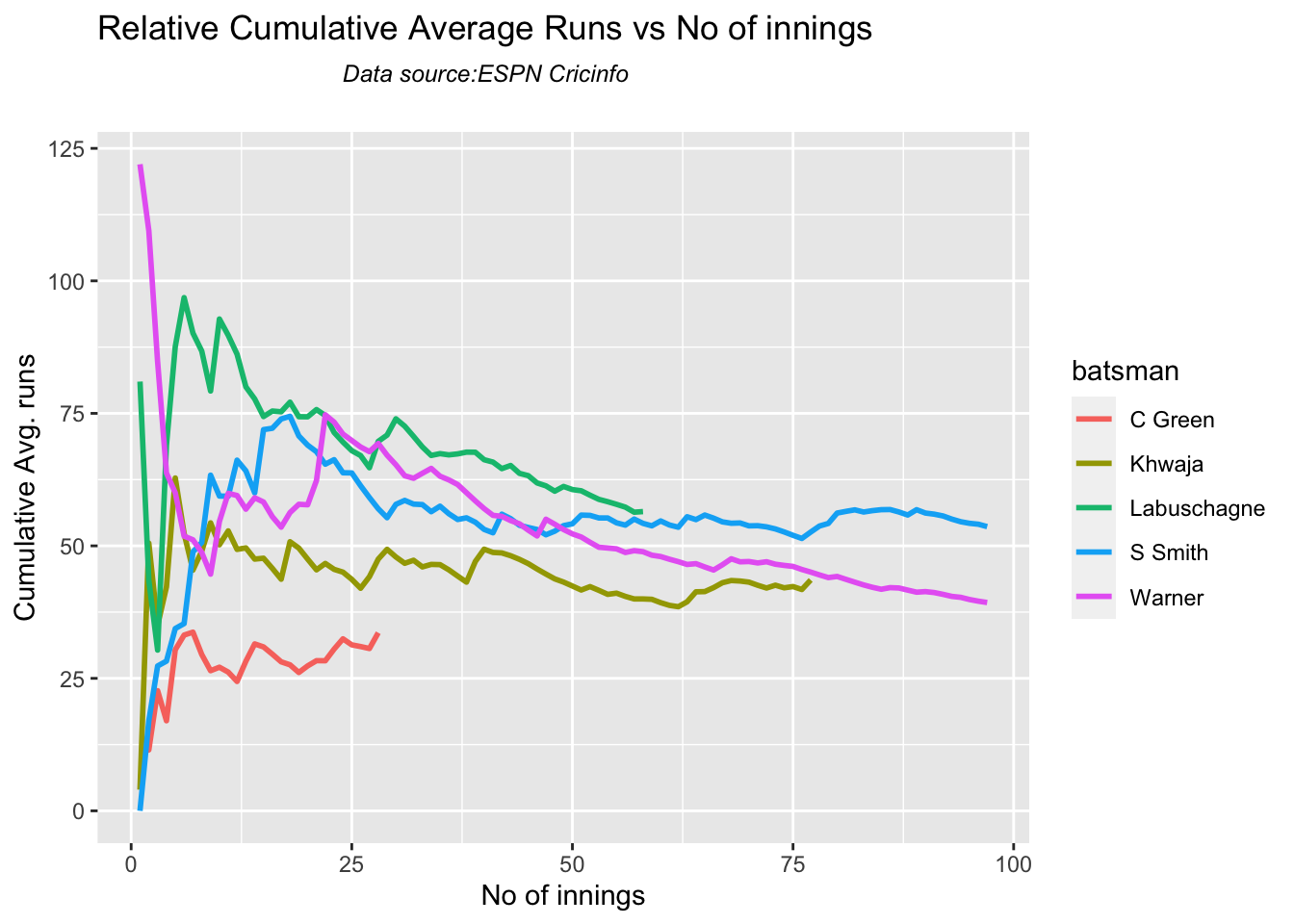
5o. Relative cumulative average runs in career

frames <- list("stevesmithTest.csv","warnerTest.csv","khwajaTest.csv","labuschagneTest.csv","cgreenTest.csv")
names <- list("S Smith","Warner","Khwaja","Labuschagne","C Green")
relativeBatsmanCumulativeAvgRuns(frames,names)

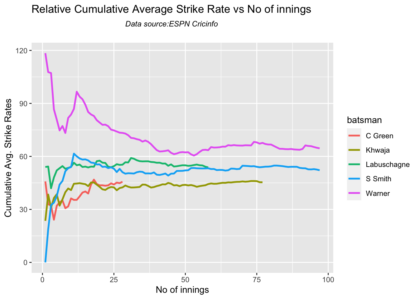
5p. Relative cumulative average strike rate in career

frames <- list("stevesmithTest.csv","warnerTest.csv","khwajaTest.csv","labuschagneTest.csv","cgreenTest.csv")
names <- list("S Smith","Warner","Khwaja","Labuschagne","C Green")
relativeBatsmanCumulativeStrikeRate(frames,names)

5q. Check Batsman In-Form or Out-of-Form

A significance value of 0.05 is chosen and p-value us computed If p-value >= .05 – Batsman In-Form If p-value < 0.05 – Batsman Out-of-Form

This is done for the Top 4 batsman

checkBatsmanInForm("stevesmith.csv","S Smith")

## [1] "**************************** Form status of S Smith ****************************\n\n Population size: 144  Mean of population: 53.76 \n Sample size: 17  Mean of sample: 45.65 SD of sample: 56.4 \n\n Null hypothesis H0 : S Smith 's sample average is within 95% confidence interval of population average\n Alternative hypothesis Ha : S Smith 's sample average is below the 95% confidence interval of population average\n\n S Smith 's Form Status: In-Form because the p value: 0.280533  is greater than alpha=  0.05 \n *******************************************************************************************\n\n"

checkBatsmanInForm("warner.csv","Warner")

## [1] "**************************** Form status of Warner ****************************\n\n Population size: 164  Mean of population: 45.2 \n Sample size: 19  Mean of sample: 26.63 SD of sample: 44.62 \n\n Null hypothesis H0 : Warner 's sample average is within 95% confidence interval of population average\n Alternative hypothesis Ha : Warner 's sample average is below the 95% confidence interval of population average\n\n Warner 's Form Status: Out-of-Form because the p value: 0.042744  is less than alpha=  0.05 \n *******************************************************************************************\n\n"

checkBatsmanInForm("labuschagne.csv","M Labuschagne")

## [1] "**************************** Form status of M Labuschagne ****************************\n\n Population size: 52  Mean of population: 59.56 \n Sample size: 6  Mean of sample: 29.67 SD of sample: 19.96 \n\n Null hypothesis H0 : M Labuschagne 's sample average is within 95% confidence interval of population average\n Alternative hypothesis Ha : M Labuschagne 's sample average is below the 95% confidence interval of population average\n\n M Labuschagne 's Form Status: Out-of-Form because the p value: 0.005239  is less than alpha=  0.05 \n *******************************************************************************************\n\n"

checkBatsmanInForm("khwaja.csv","Khwaja")

## [1] "**************************** Form status of Khwaja ****************************\n\n Population size: 89  Mean of population: 41.62 \n Sample size: 10  Mean of sample: 53.1 SD of sample: 76.34 \n\n Null hypothesis H0 : Khwaja 's sample average is within 95% confidence interval of population average\n Alternative hypothesis Ha : Khwaja 's sample average is below the 95% confidence interval of population average\n\n Khwaja 's Form Status: In-Form because the p value: 0.677691  is greater than alpha=  0.05 \n *******************************************************************************************\n\n"

5r. Predicting Runs given Balls Faced and Minutes at Crease

A multi-variate regression plane is fitted between Runs and Balls faced +Minutes at crease.

BF <- seq( 10, 400,length=15)
Mins <- seq(30,600,length=15)
newDF <- data.frame(BF,Mins)
ssmith1 <- batsmanRunsPredict("stevesmith.csv","S Smith",newdataframe=newDF)

warner1 <- batsmanRunsPredict("warner.csv","Warner",newdataframe=newDF)

khwaja1 <- batsmanRunsPredict("khwaja.csv","Khwaja",newdataframe=newDF)
labuschagne1 <- batsmanRunsPredict("labuschagne.csv","Labuschagne",newdataframe=newDF)

cgreen1 <- batsmanRunsPredict("cgreen.csv","C Green",newdataframe=newDF)

batsmen <-cbind(round(ssmith1$Runs),round(warner1$Runs),round(khwaja1$Runs),round(labuschagne1$Runs),round(cgreen1$Runs))
colnames(batsmen) <- c("S Smith","Warner","Khwaja","Labuschagne","C Green")
newDF <- data.frame(round(newDF$BF),round(newDF$Mins))
colnames(newDF) <- c("BallsFaced","MinsAtCrease")
predictedRuns <- cbind(newDF,batsmen)
predictedRuns

##    BallsFaced MinsAtCrease S Smith Warner Khwaja Labuschagne C Green
## 1          10           30       7     10     10           9      13
## 2          38           71      23     30     24          24      29
## 3          66          111      38     50     38          40      44
## 4          94          152      53     70     53          55      60
## 5         121          193      69     90     67          70      75
## 6         149          234      84    110     81          85      91
## 7         177          274     100    130     95         100     106
## 8         205          315     115    150    109         116     122
## 9         233          356     130    170    123         131     137
## 10        261          396     146    190    137         146     153
## 11        289          437     161    210    151         161     168
## 12        316          478     177    230    165         176     184
## 13        344          519     192    250    179         192     199
## 14        372          559     207    270    193         207     215
## 15        400          600     223    290    207         222     230

6. Analysis of Australia WTC batsmen from Jan 2016 – May 2023 against India

6a. Relative cumulative average runs in career

Labuschagne, Smith and C Green have good records against India

frames <- list("stevesmithTestInd.csv","warnerTestInd.csv","khwajaTestInd.csv","labuschagneTestInd.csv","cgreenTestInd.csv")
names <- list("S Smith","Warner","Khwaja","Labuschagne","C Green")
relativeBatsmanCumulativeAvgRuns(frames,names)

6b. Relative cumulative average strike rate in career

Warner, Labuschagne and Smith have a good strike rate against India

frames <- list("stevesmithTestInd.csv","warnerTestInd.csv","khwajaTestInd.csv","labuschagneTestInd.csv","cgreenTestInd.csv")
names <- list("S Smith","Warner","Khwaja","Labuschagne","C Green")
relativeBatsmanCumulativeStrikeRate(frames,names)

7. Analysis of India WTC bowlers from Jan 2016 – May 2023

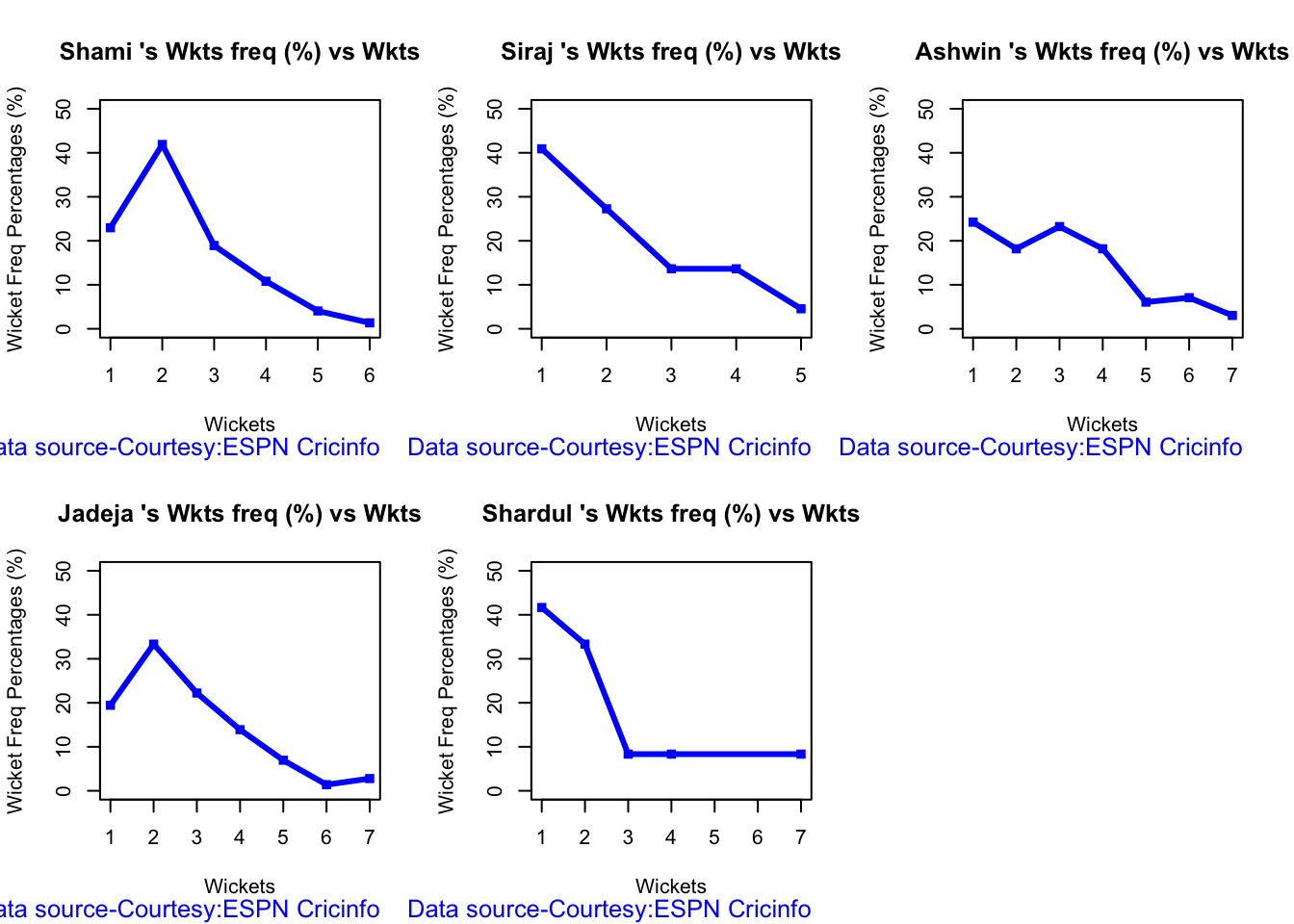
7a Wickets frequency chart

par(mfrow=c(2,3))
par(mar=c(4,4,2,2))
bowlerWktsFreqPercent("shamiTest.csv","Shami")
bowlerWktsFreqPercent("sirajTest.csv","Siraj")
bowlerWktsFreqPercent("ashwinTest.csv","Ashwin")
bowlerWktsFreqPercent("jadejaTest.csv","Jadeja")
bowlerWktsFreqPercent("shardulTest.csv","Shardul")

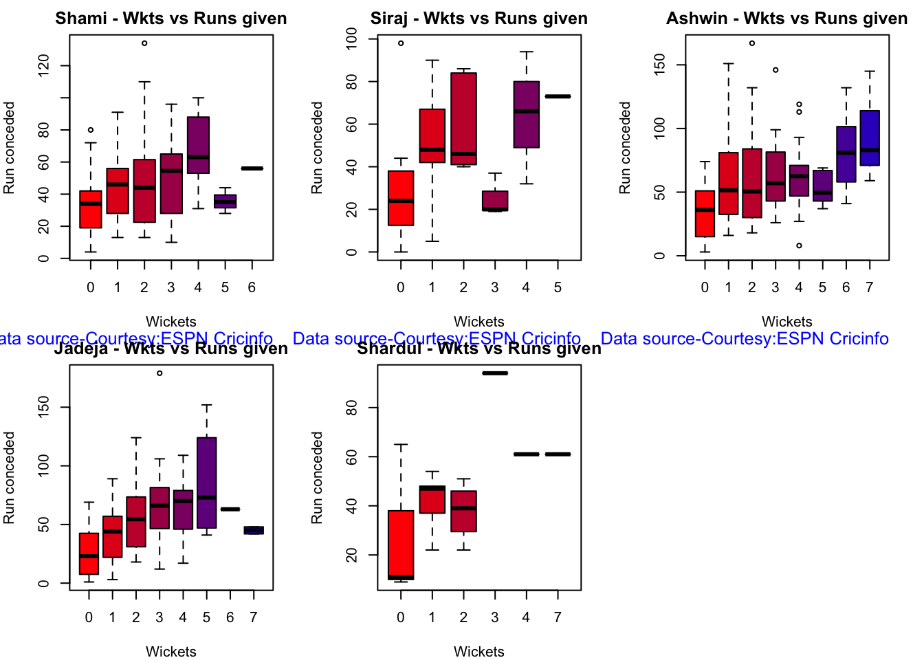
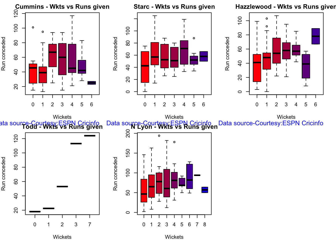
7b Wickets Runs chart

par(mfrow=c(2,3))
par(mar=c(4,4,2,2))

bowlerWktsRunsPlot("shamiTest.csv","Shami")
bowlerWktsRunsPlot("sirajTest.csv","Siraj")
bowlerWktsRunsPlot("ashwinTest.csv","Ashwin")
bowlerWktsRunsPlot("jadejaTest.csv","Jadeja")
bowlerWktsRunsPlot("shardulTest.csv","Shardul")

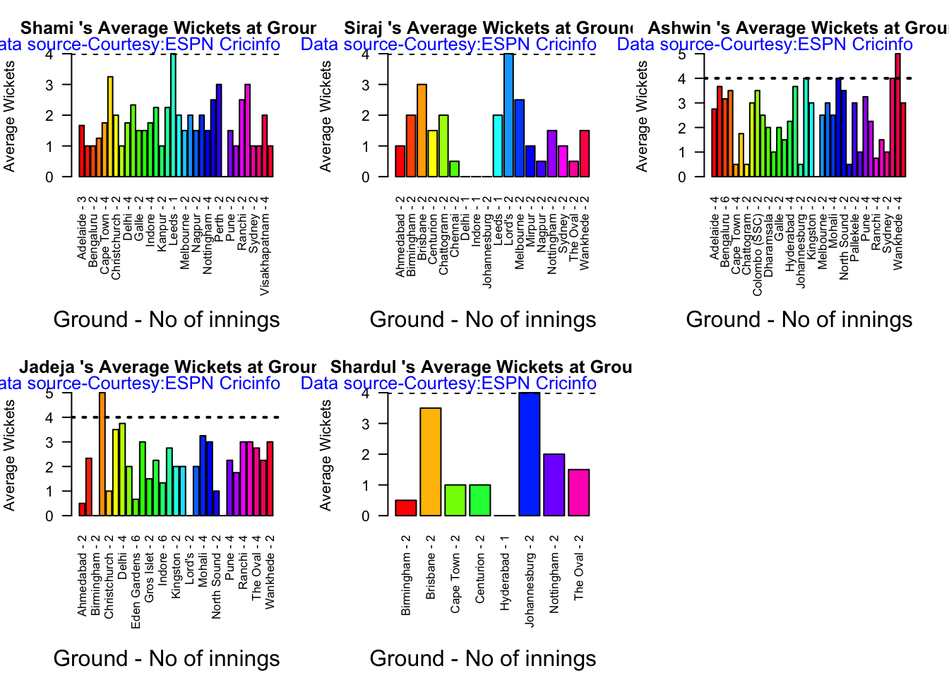
7c. Average wickets at different venues

par(mfrow=c(2,3))
par(mar=c(4,4,2,2))

bowlerAvgWktsGround("shamiTest.csv","Shami")
bowlerAvgWktsGround("sirajTest.csv","Siraj")
bowlerAvgWktsGround("ashwinTest.csv","Ashwin")
bowlerAvgWktsGround("jadejaTest.csv","Jadeja")
bowlerAvgWktsGround("shardulTest.csv","Shardul")

7d Average wickets against different opposition

par(mfrow=c(2,3))
par(mar=c(4,4,2,2))

bowlerAvgWktsOpposition("shamiTest.csv","Shami")
bowlerAvgWktsOpposition("sirajTest.csv","Siraj")
bowlerAvgWktsOpposition("ashwinTest.csv","Ashwin")
bowlerAvgWktsOpposition("jadejaTest.csv","Jadeja")
bowlerAvgWktsOpposition("shardulTest.csv","Shardul")

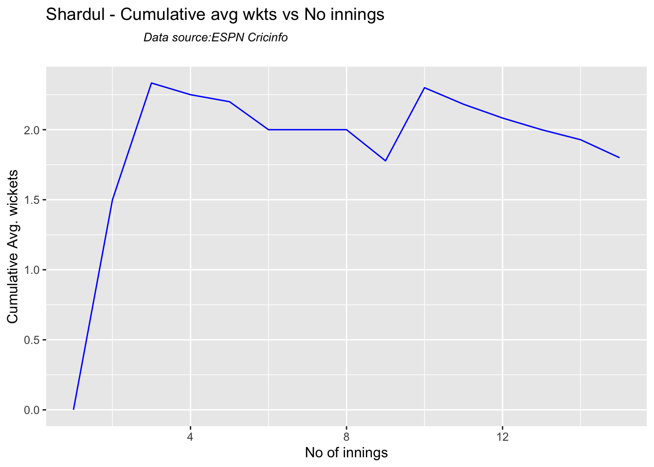
7e Cumulative average wickets taken

Ashwin’s performance has dropped over the years, while Siraj has been becoming better

par(mfrow=c(2,2))
par(mar=c(4,4,2,2))

bowlerCumulativeAvgWickets("shamiTest.csv","Shami")

bowlerCumulativeAvgWickets("sirajTest.csv","Siraj")

bowlerCumulativeAvgWickets("ashwinTest.csv","Ashwin")

bowlerCumulativeAvgWickets("jadejaTest.csv","Jadeja")

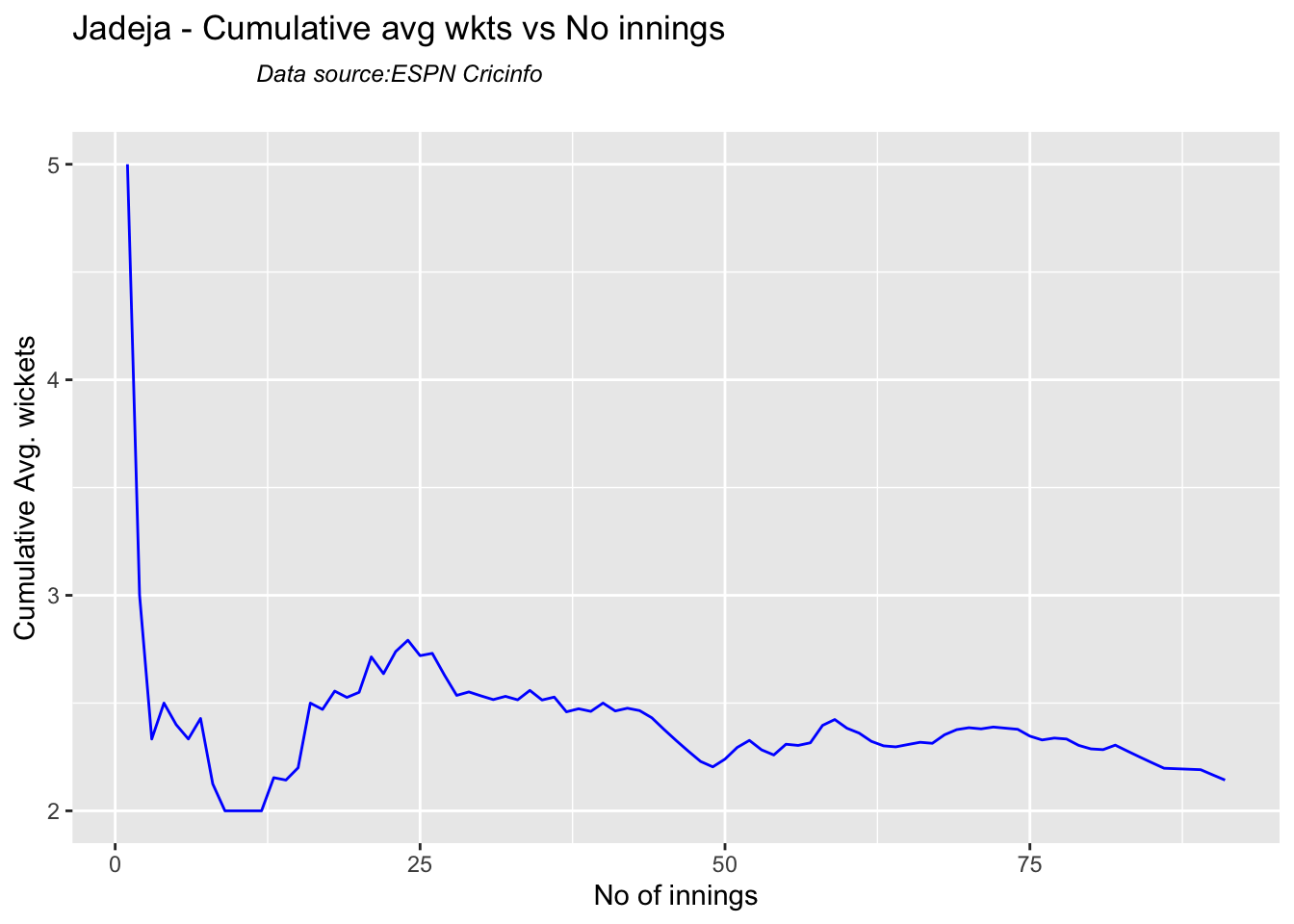
bowlerCumulativeAvgWickets("shardulTest.csv","Shardul")

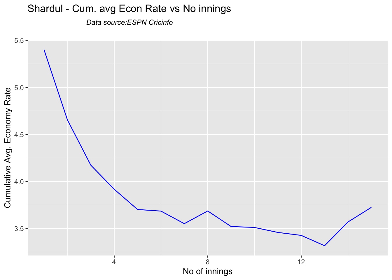
7g Cumulative average economy rate

par(mfrow=c(2,3))
par(mar=c(4,4,2,2))

bowlerCumulativeAvgEconRate("shamiTest.csv","Shami")

bowlerCumulativeAvgEconRate("sirajTest.csv","Siraj")

bowlerCumulativeAvgEconRate("ashwinTest.csv","Ashwin")

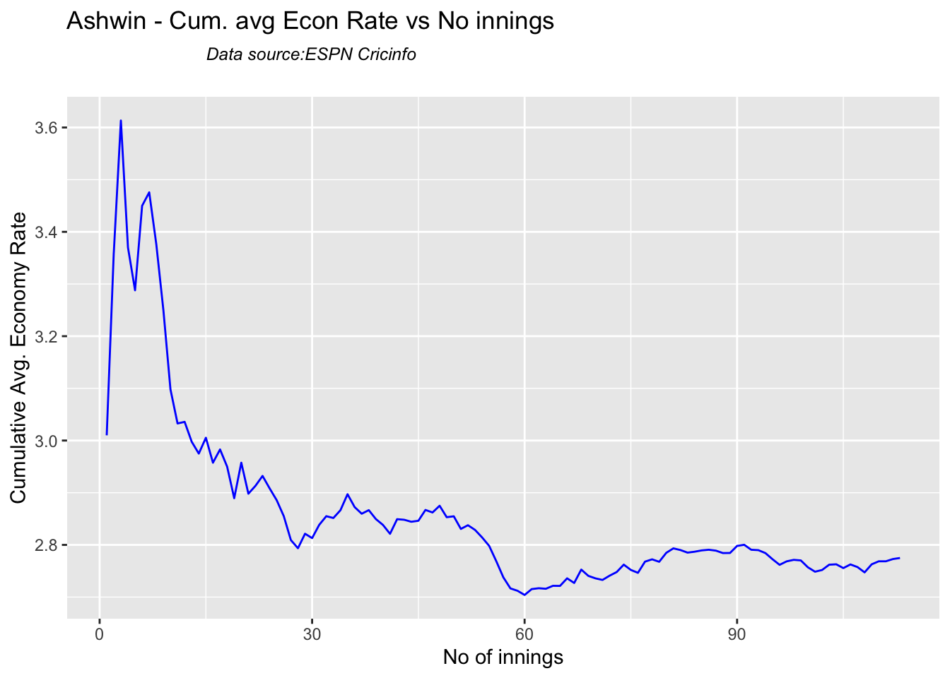
bowlerCumulativeAvgEconRate("jadejaTest.csv","Jadeja")

bowlerCumulativeAvgEconRate("shardulTest.csv","Shardul")

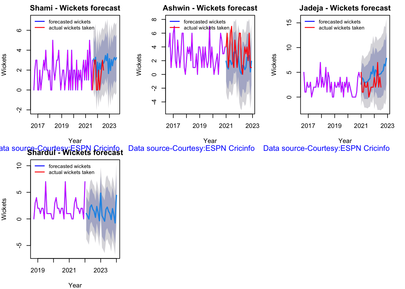
7h Wicket forecast

Here are plots that forecast how the bowler will perform in future. In this case 90% of the career wickets trend is used as the training set. the remaining 10% is the test set.

A Holt-Winters forecasting model is used to forecast future performance based on the 90% training set. The forecasted wickets trend is plotted. The test set is also plotted to see how close the forecast and the actual matches

par(mfrow=c(2,3))
par(mar=c(4,4,2,2))

bowlerPerfForecast("shamiTest.csv","Shami")
#bowlerPerfForecast("sirajTest.csv","Siraj")
bowlerPerfForecast("ashwinTest.csv","Ashwin")
bowlerPerfForecast("jadejaTest.csv","Jadeja")
bowlerPerfForecast("shardulTest.csv","Shardul")

7i Relative Wickets Frequency Percentage

frames <- list("shamiTest.csv","sirajTest.csv","ashwinTest.csv","jadejaTest.csv","shardulTest.csv")
names <- list("Shami","Siraj","Ashwin","Jadeja","Shardul")
relativeBowlingPerf(frames,names)

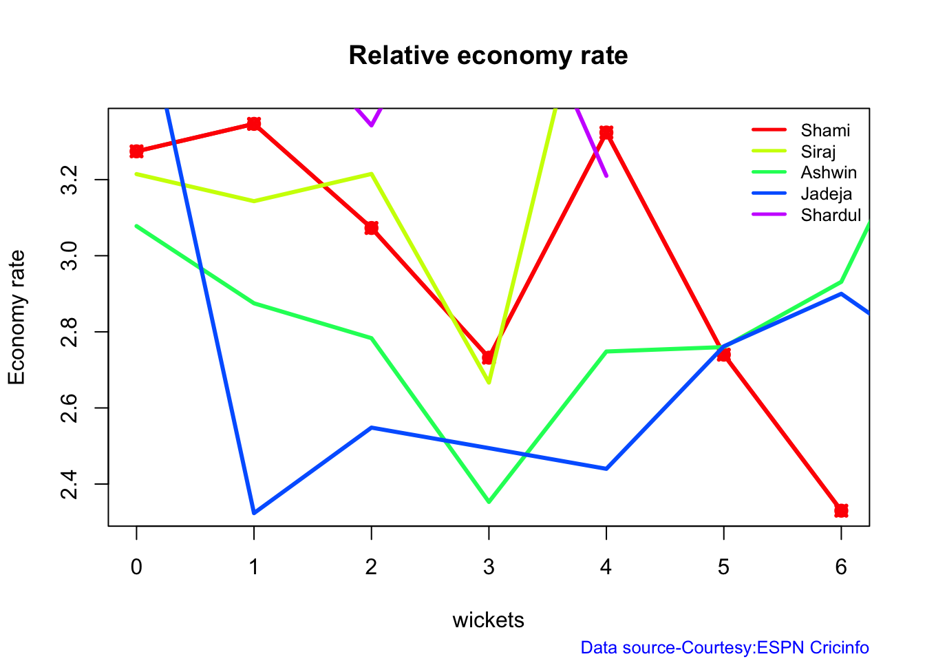
7j Relative Economy Rate against wickets taken

frames <- list("shamiTest.csv","sirajTest.csv","ashwinTest.csv","jadejaTest.csv","shardulTest.csv")
names <- list("Shami","Siraj","Ashwin","Jadeja","Shardul")
relativeBowlingER(frames,names)

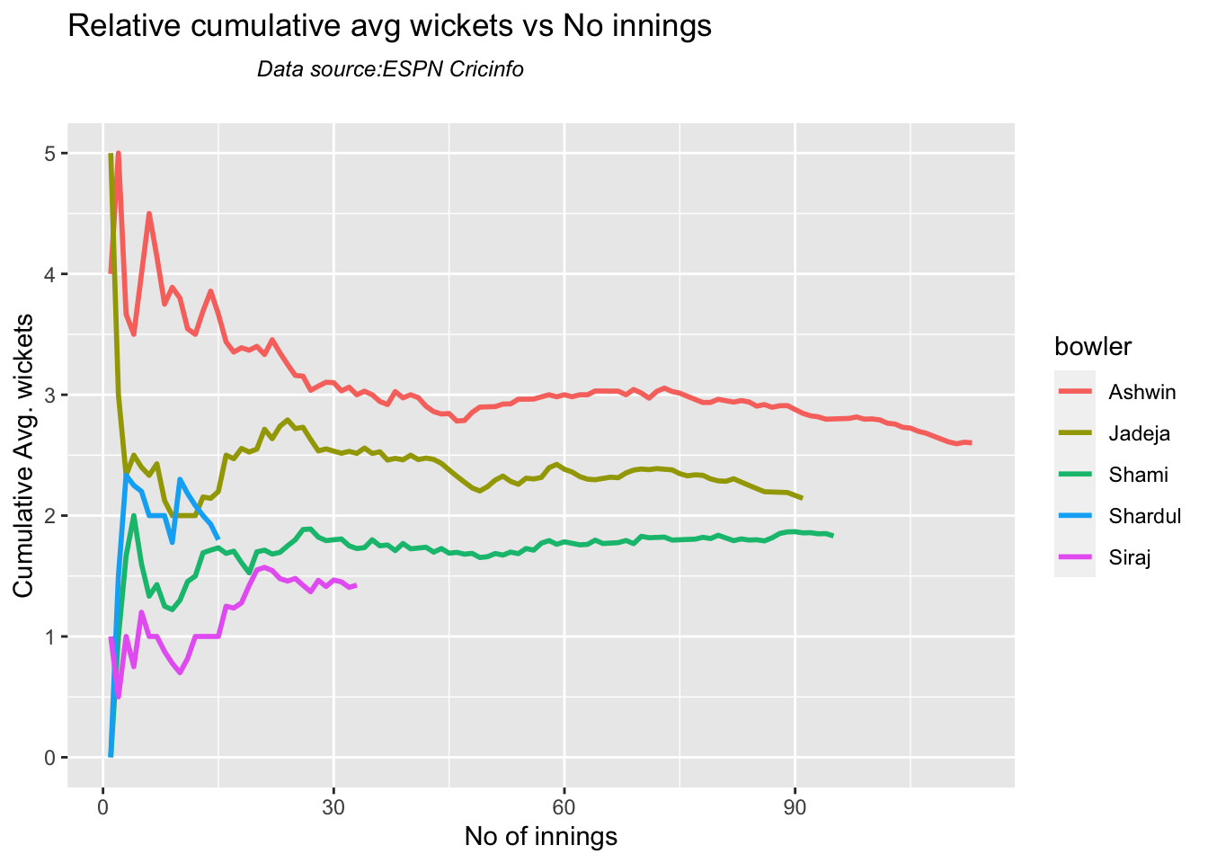
7k Relative cumulative average wickets of bowlers in career

Ashwin has the highest wickets followed by Jadeja against all teams

frames <- list("shamiTest.csv","sirajTest.csv","ashwinTest.csv","jadejaTest.csv","shardulTest.csv")
names <- list("Shami","Siraj","Ashwin","Jadeja","Shardul")
relativeBowlerCumulativeAvgWickets(frames,names)

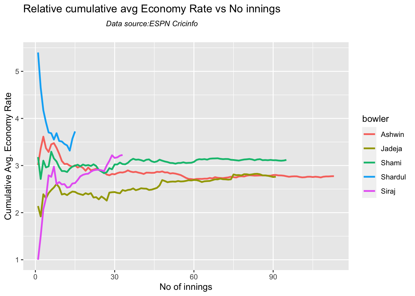
7l Relative cumulative average economy rate of bowlers

Jadeja has the best economy rate followed by Ashwin

frames <- list("shamiTest.csv","sirajTest.csv","ashwinTest.csv","jadejaTest.csv","shardulTest.csv")
names <- list("Shami","Siraj","Ashwin","Jadeja","Shardul")
relativeBowlerCumulativeAvgEconRate(frames,names)

7m Check for bowler in-form/out-of-form

The below computation uses Null Hypothesis testing and p-value to determine if the bowler is in-form or out-of-form. For this 90% of the career wickets is chosen as the population and the mean computed. The last 10% is chosen to be the sample set and the sample Mean and the sample Standard Deviation are caculated.

The Null Hypothesis (H0) assumes that the bowler continues to stay in-form where the sample mean is within 95% confidence interval of population mean The Alternative (Ha) assumes that the bowler is out of form the sample mean is beyond the 95% confidence interval of the population mean.

A significance value of 0.05 is chosen and p-value us computed If p-value >= .05 – Batsman In-Form If p-value < 0.05 – Batsman Out-of-Form

Note: The check for the form status of the bowlers indicate

checkBowlerInForm("shami.csv","Shami")

## [1] "**************************** Form status of Shami ****************************\n\n Population size: 106  Mean of population: 1.93 \n Sample size: 12  Mean of sample: 1.33 SD of sample: 1.23 \n\n Null hypothesis H0 : Shami 's sample average is within 95% confidence interval \n        of population average\n Alternative hypothesis Ha : Shami 's sample average is below the 95% confidence\n        interval of population average\n\n Shami 's Form Status: In-Form because the p value: 0.058427  is greater than alpha=  0.05 \n *******************************************************************************************\n\n"

checkBowlerInForm("siraj.csv","Siraj")

## [1] "**************************** Form status of Siraj ****************************\n\n Population size: 29  Mean of population: 1.59 \n Sample size: 4  Mean of sample: 0.25 SD of sample: 0.5 \n\n Null hypothesis H0 : Siraj 's sample average is within 95% confidence interval \n        of population average\n Alternative hypothesis Ha : Siraj 's sample average is below the 95% confidence\n        interval of population average\n\n Siraj 's Form Status: Out-of-Form because the p value: 0.002923  is less than alpha=  0.05 \n *******************************************************************************************\n\n"

checkBowlerInForm("ashwin.csv","Ashwin")

## [1] "**************************** Form status of Ashwin ****************************\n\n Population size: 154  Mean of population: 2.77 \n Sample size: 18  Mean of sample: 2.44 SD of sample: 1.76 \n\n Null hypothesis H0 : Ashwin 's sample average is within 95% confidence interval \n        of population average\n Alternative hypothesis Ha : Ashwin 's sample average is below the 95% confidence\n        interval of population average\n\n Ashwin 's Form Status: In-Form because the p value: 0.218345  is greater than alpha=  0.05 \n *******************************************************************************************\n\n"

checkBowlerInForm("jadeja.csv","Jadeja")

## [1] "**************************** Form status of Jadeja ****************************\n\n Population size: 108  Mean of population: 2.22 \n Sample size: 12  Mean of sample: 1.92 SD of sample: 2.35 \n\n Null hypothesis H0 : Jadeja 's sample average is within 95% confidence interval \n        of population average\n Alternative hypothesis Ha : Jadeja 's sample average is below the 95% confidence\n        interval of population average\n\n Jadeja 's Form Status: In-Form because the p value: 0.333095  is greater than alpha=  0.05 \n *******************************************************************************************\n\n"

checkBowlerInForm("shardul.csv","Shardul")

## [1] "**************************** Form status of Shardul ****************************\n\n Population size: 13  Mean of population: 2 \n Sample size: 2  Mean of sample: 0.5 SD of sample: 0.71 \n\n Null hypothesis H0 : Shardul 's sample average is within 95% confidence interval \n        of population average\n Alternative hypothesis Ha : Shardul 's sample average is below the 95% confidence\n        interval of population average\n\n Shardul 's Form Status: Out-of-Form because the p value: 0.04807  is less than alpha=  0.05 \n *******************************************************************************************\n\n"

8. Analysis of India WTC bowlers from Jan 2016 – May 2023 against Australia

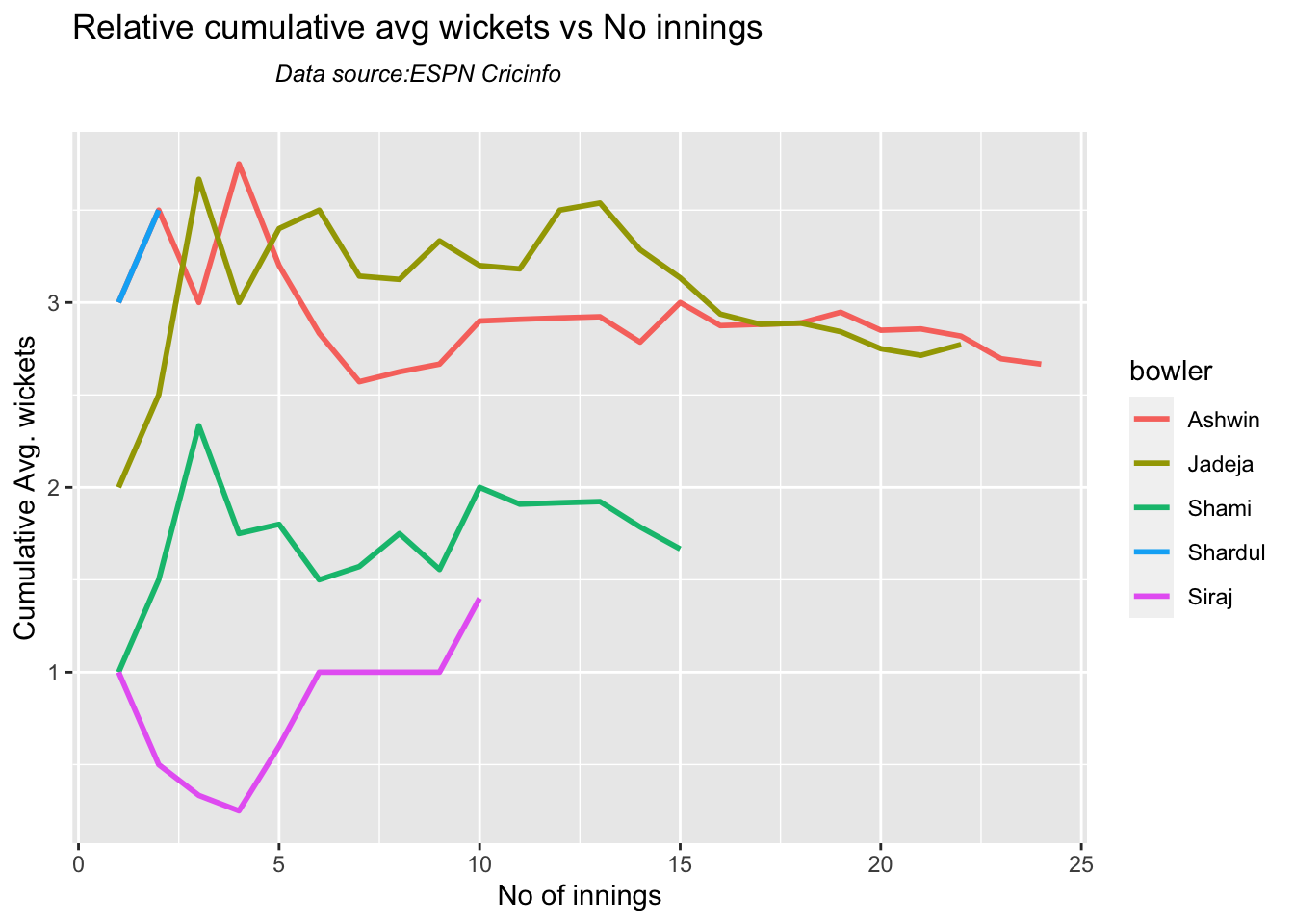
8a Relative cumulative average wickets of bowlers in career

Against Australia specifically Jadeja has the best record followed by Ashwin

frames <- list("shamiTestAus.csv","sirajTestAus.csv","ashwinTestAus.csv","jadejaTestAus.csv","shardulTestAus.csv")
names <- list("Shami","Siraj","Ashwin","Jadeja","Shardul")
relativeBowlerCumulativeAvgWickets(frames,names)

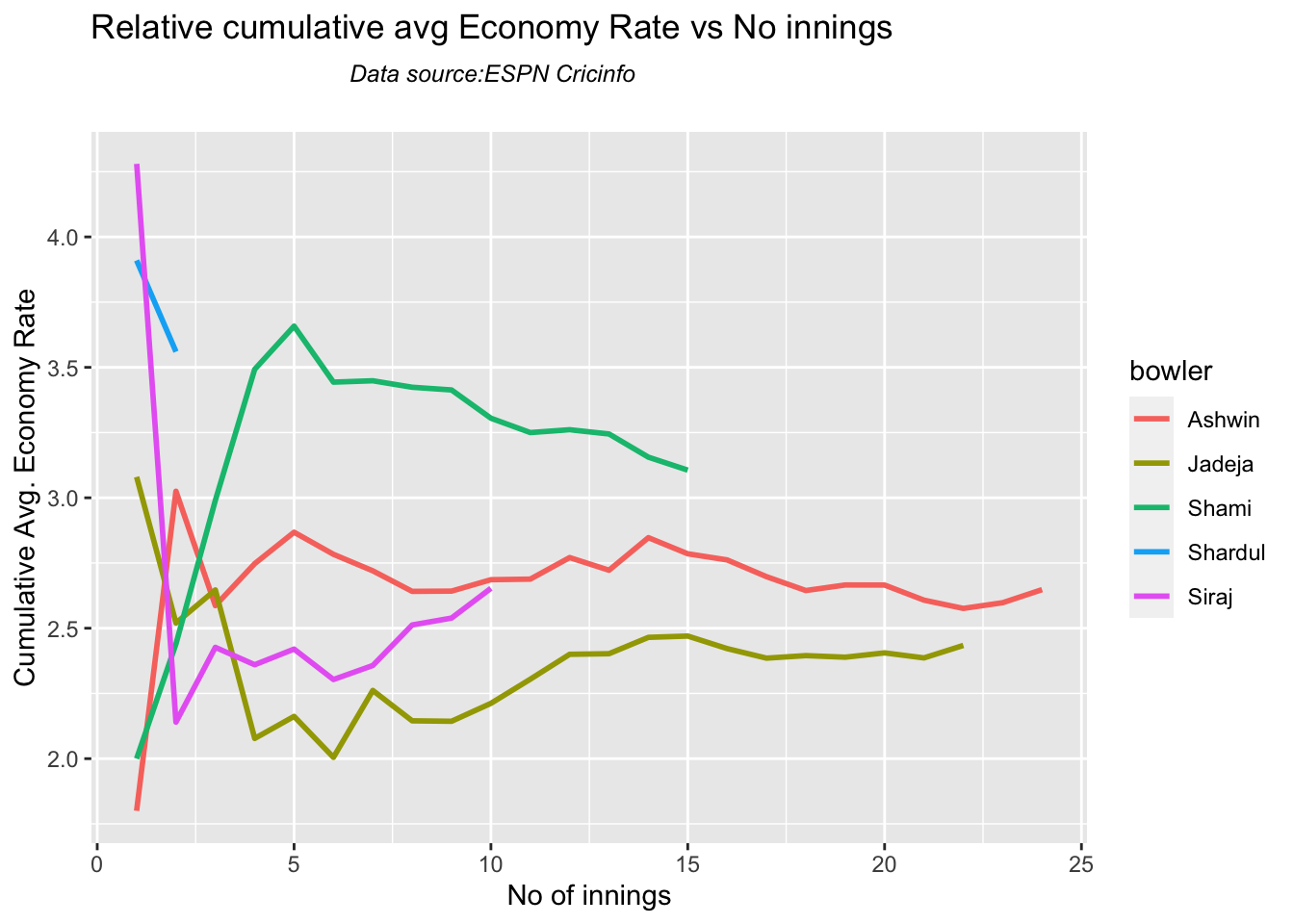
8b Relative cumulative average economy rate of bowlers

Jadeja has the best economy followed by Siraj, then Ashwin

frames <- list("shamiTestAus.csv","sirajTestAus.csv","ashwinTestAus.csv","jadejaTestAus.csv","shardulTestAus.csv")
names <- list("Shami","Siraj","Ashwin","Jadeja","Shardul")
relativeBowlerCumulativeAvgEconRate(frames,names)

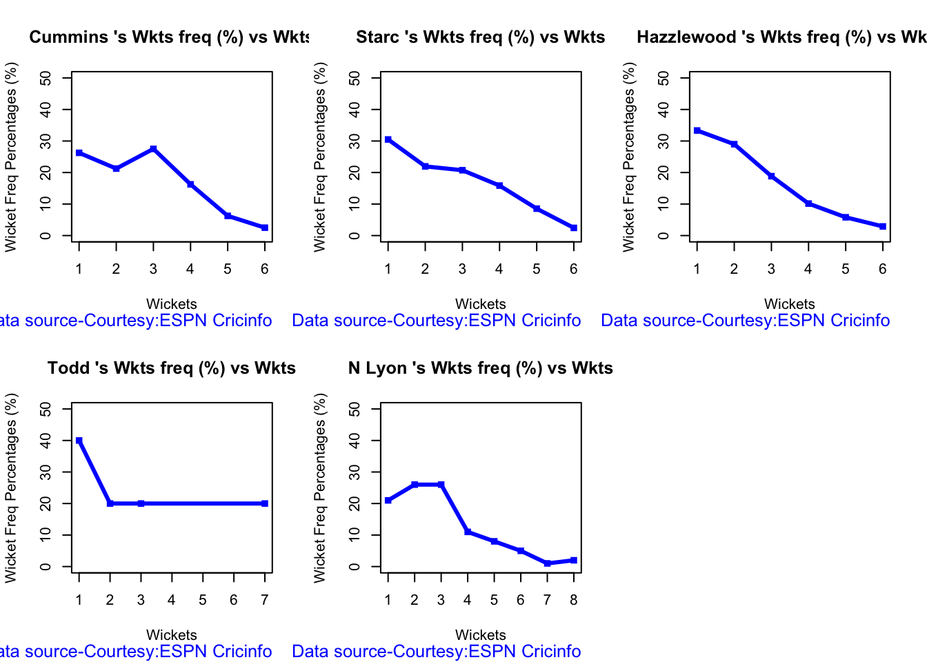
8. Analysis of India WTC bowlers from Jan 2016 – May 2023

8a. Wickets frequency chart

par(mfrow=c(2,3))
par(mar=c(4,4,2,2))
bowlerWktsFreqPercent("cumminsTest.csv","Cummins")
bowlerWktsFreqPercent("starcTest.csv","Starc")
bowlerWktsFreqPercent("hazzlewoodTest.csv","Hazzlewood")
bowlerWktsFreqPercent("todd.csv","Todd")
bowlerWktsFreqPercent("lyonTest.csv","N Lyon")

8b. Wickets frequency chart

par(mfrow=c(2,3))
par(mar=c(4,4,2,2))

bowlerWktsRunsPlot("cumminsTest.csv","Cummins")
bowlerWktsRunsPlot("starcTest.csv","Starc")
bowlerWktsRunsPlot("hazzlewoodTest.csv","Hazzlewood")
bowlerWktsRunsPlot("todd.csv","Todd")
bowlerWktsRunsPlot("lyonTest.csv","N Lyon")

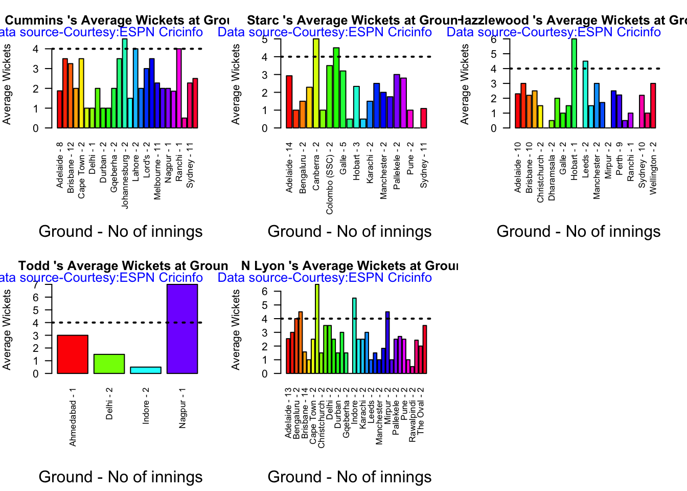
8c. Average wickets at different venues

par(mfrow=c(2,3))
par(mar=c(4,4,2,2))

bowlerAvgWktsGround("cumminsTest.csv","Cummins")
bowlerAvgWktsGround("starcTest.csv","Starc")
bowlerAvgWktsGround("hazzlewoodTest.csv","Hazzlewood")
bowlerAvgWktsGround("todd.csv","Todd")
bowlerAvgWktsGround("lyonTest.csv","N Lyon")

8d Average wickets against different opposition

par(mfrow=c(2,3))
par(mar=c(4,4,2,2))

bowlerAvgWktsOpposition("cumminsTest.csv","Cummins")
bowlerAvgWktsOpposition("starcTest.csv","Starc")
bowlerAvgWktsOpposition("hazzlewoodTest.csv","Hazzlewood")
bowlerAvgWktsOpposition("todd.csv","Todd")
bowlerAvgWktsOpposition("lyonTest.csv","N Lyon")

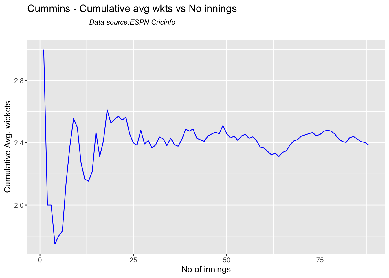
8e Cumulative average wickets taken

par(mfrow=c(2,2))
par(mar=c(4,4,2,2))

bowlerCumulativeAvgWickets("cumminsTest.csv","Cummins")

bowlerCumulativeAvgWickets("starcTest.csv","Starc")

bowlerCumulativeAvgWickets("hazzlewoodTest.csv","Hazzlewood")

bowlerCumulativeAvgWickets("todd.csv","Todd")

bowlerCumulativeAvgWickets("lyonTest.csv","N Lyon")

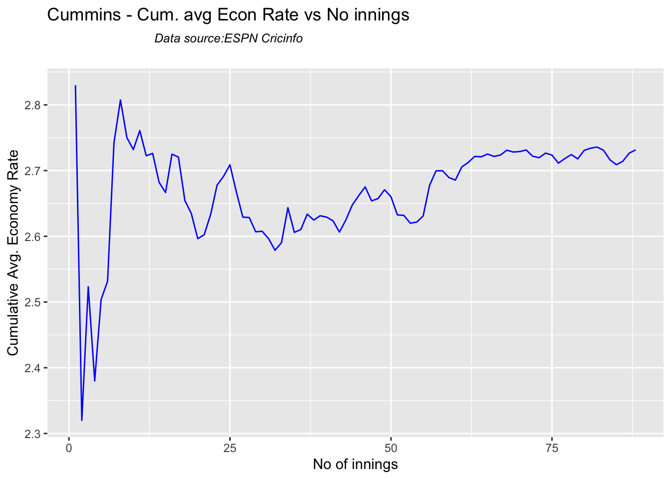
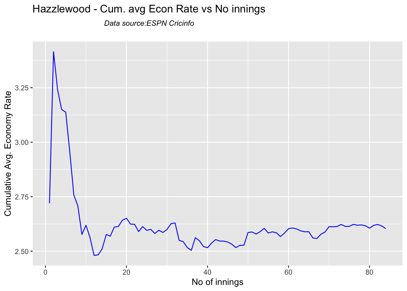
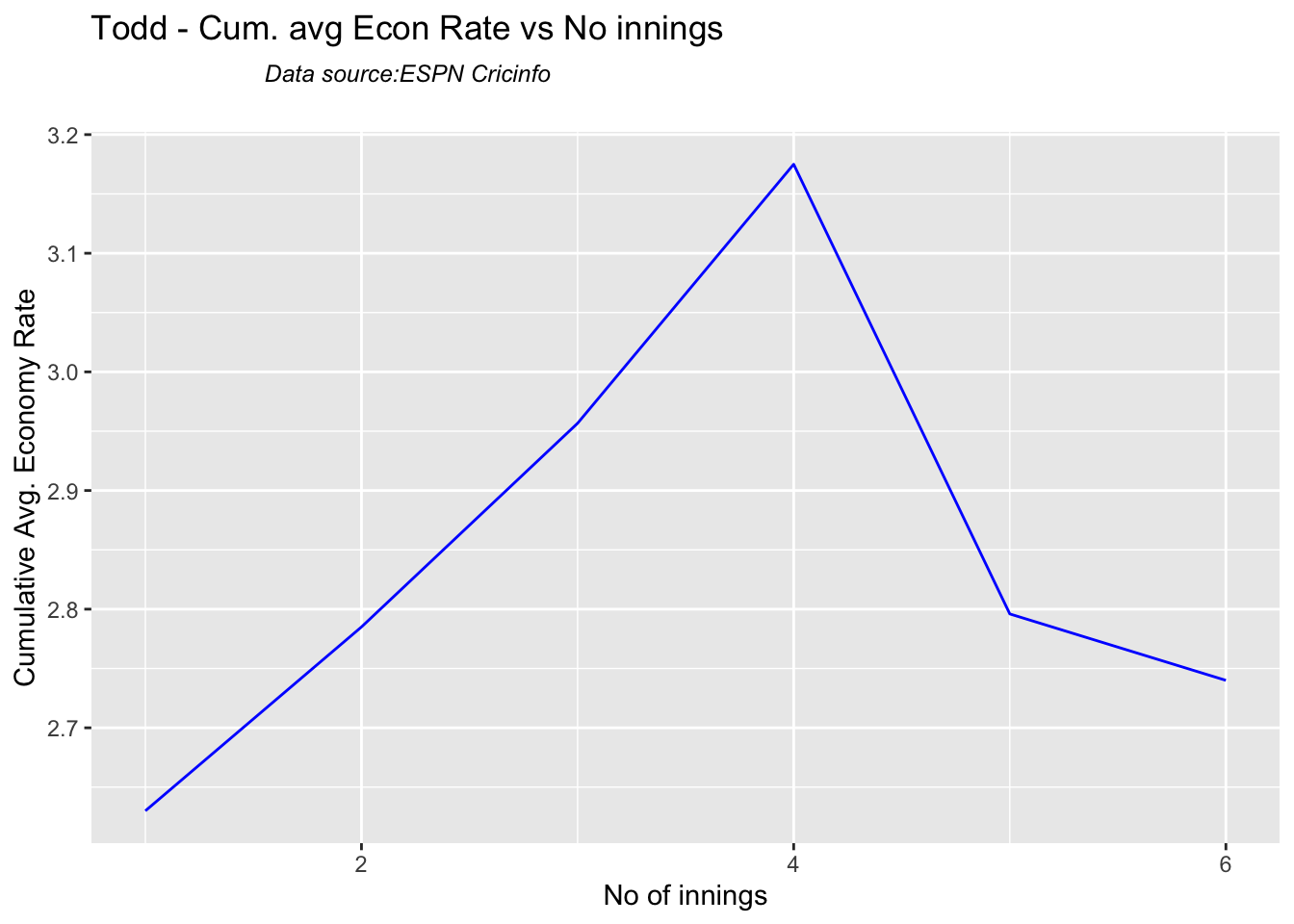
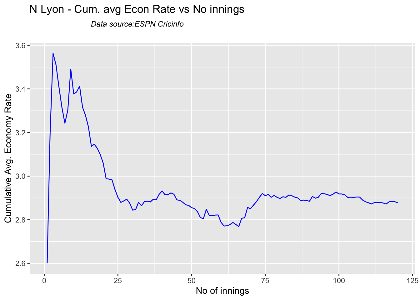
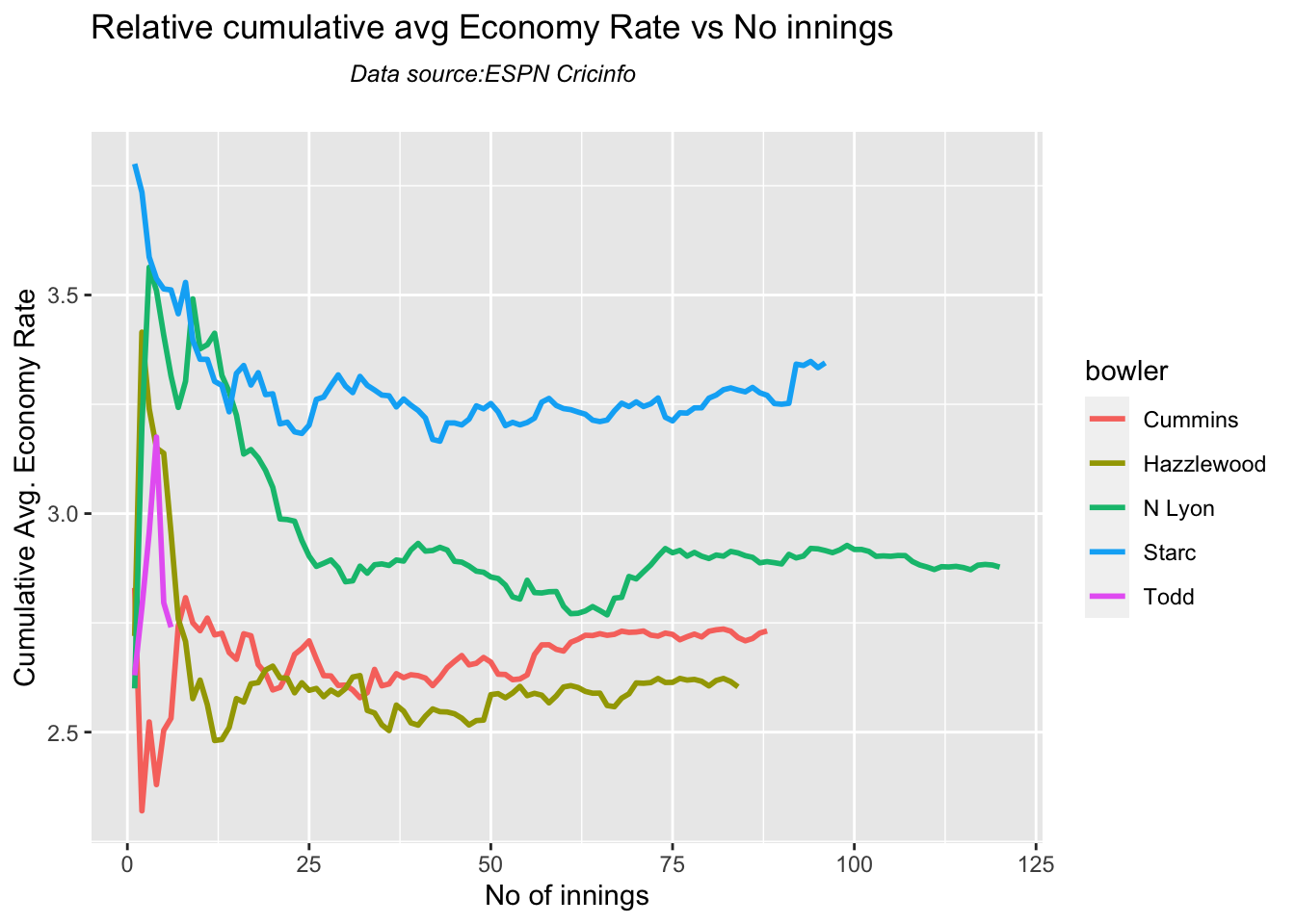
8g Cumulative average economy rate

par(mfrow=c(2,3))
par(mar=c(4,4,2,2))

bowlerCumulativeAvgEconRate("cumminsTest.csv","Cummins")

bowlerCumulativeAvgEconRate("starcTest.csv","Starc")

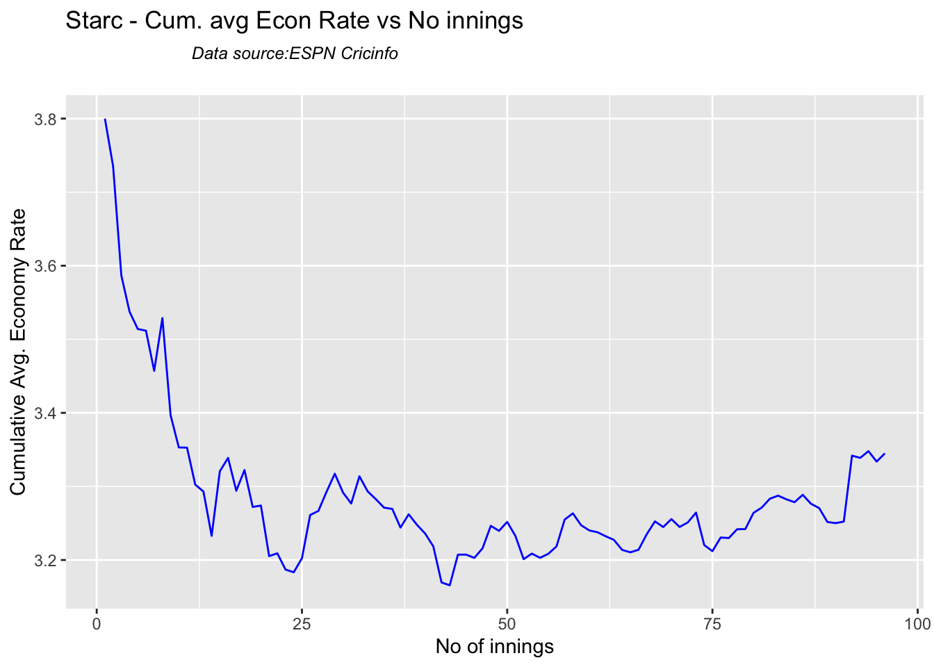
bowlerCumulativeAvgEconRate("hazzlewoodTest.csv","Hazzlewood")

bowlerCumulativeAvgEconRate("todd.csv","Todd")

bowlerCumulativeAvgEconRate("lyonTest.csv","N Lyon")

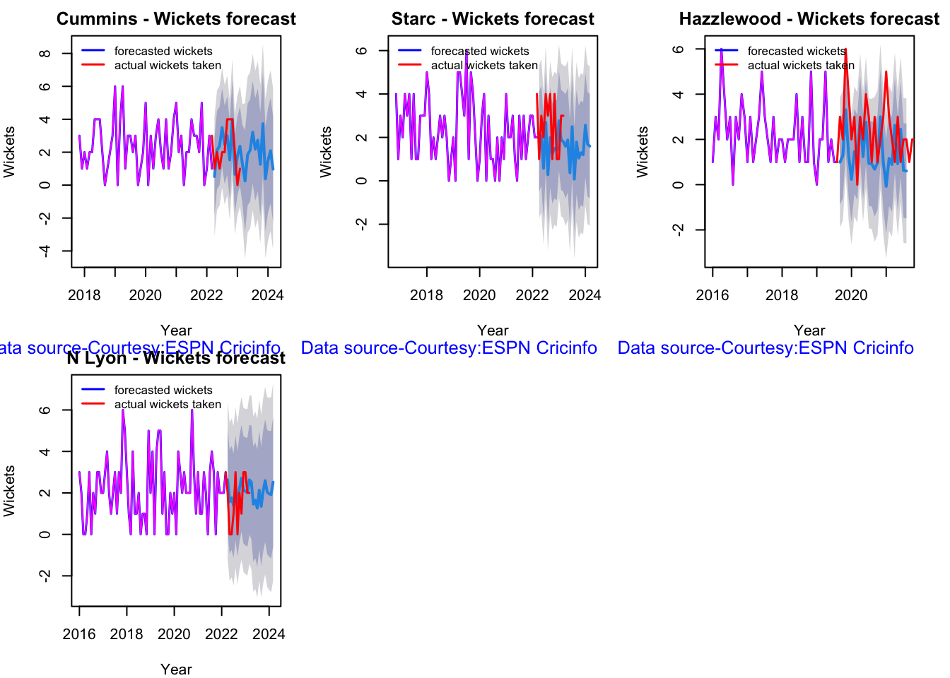
8f. Future Wickets forecast

Here are plots that forecast how the bowler will perform in future. In this case 90% of the career wickets trend is used as the training set. the remaining 10% is the test set.

A Holt-Winters forecasting model is used to forecast future performance based on the 90% training set. The forecated wickets trend is plotted. The test set is also plotted to see how close the forecast and the actual matches

par(mfrow=c(2,3))
par(mar=c(4,4,2,2))

bowlerPerfForecast("cumminsTest.csv","Cummins")
bowlerPerfForecast("starcTest.csv","Starc")
bowlerPerfForecast("hazzlewoodTest.csv","Hazzlewood")
bowlerPerfForecast("lyonTest.csv","N Lyon")

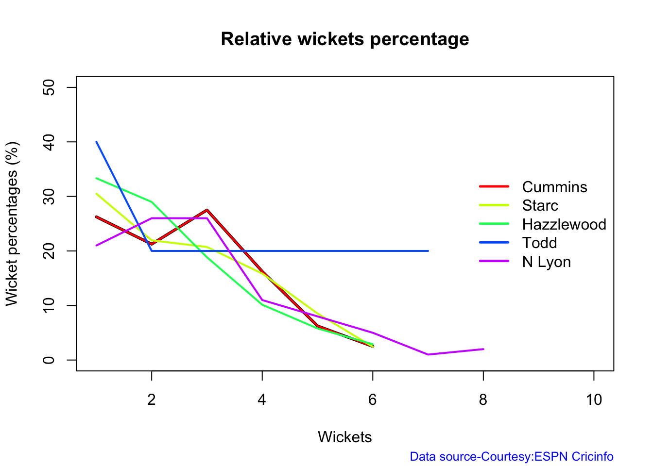
8i. Relative Wickets Frequency Percentage

frames <- list("cumminsTest.csv","starcTest.csv","hazzlewoodTest.csv","todd.csv","lyonTest.csv")
names <- list("Cummins","Starc","Hazzlewood","Todd","N Lyon")
relativeBowlingPerf(frames,names)

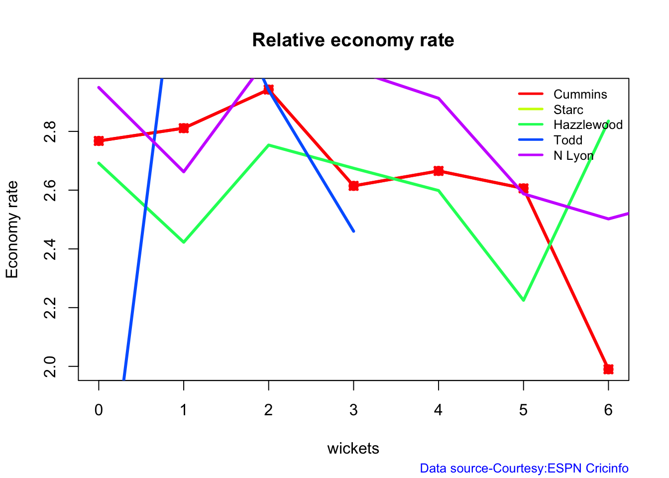
8j Relative Economy Rate against wickets taken

frames <- list("cumminsTest.csv","starcTest.csv","hazzlewoodTest.csv","todd.csv","lyonTest.csv")
names <- list("Cummins","Starc","Hazzlewood","Todd","N Lyon")
relativeBowlingER(frames,names)

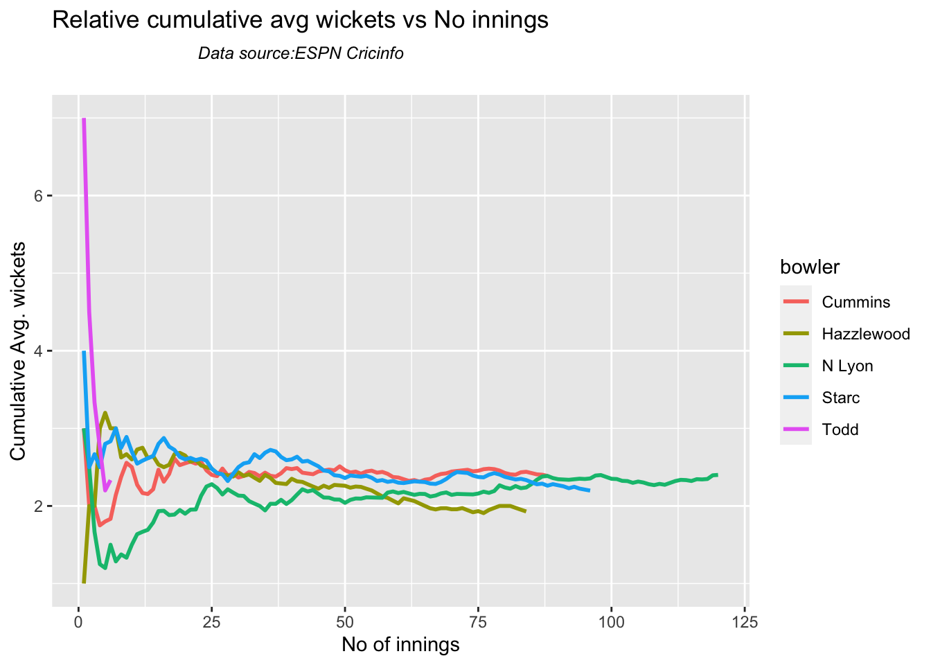
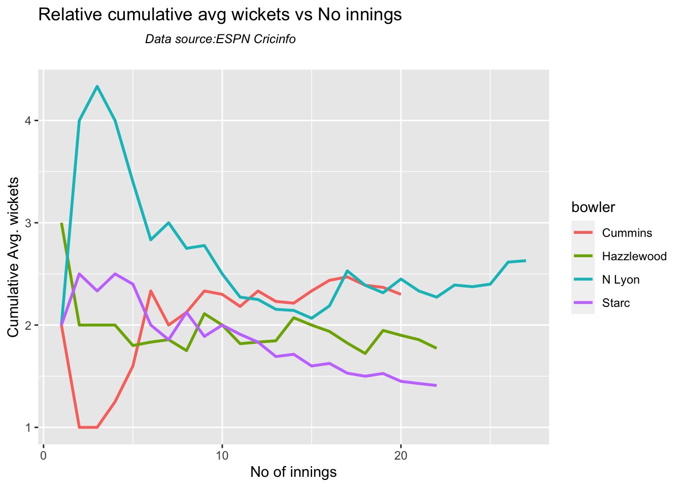
8k Relative cumulative average wickets of bowlers in career

Cummins, Starc and Lyons are the best performers

frames <- list("cumminsTest.csv","starcTest.csv","hazzlewoodTest.csv","todd.csv","lyonTest.csv")
names <- list("Cummins","Starc","Hazzlewood","Todd","N Lyon")
relativeBowlerCumulativeAvgWickets(frames,names)

8l Relative cumulative average economy rate of bowlers

Hazzlewood, Cummins have the best economy against all oppostion

frames <- list("cumminsTest.csv","starcTest.csv","hazzlewoodTest.csv","todd.csv","lyonTest.csv")
names <- list("Cummins","Starc","Hazzlewood","Todd","N Lyon")
relativeBowlerCumulativeAvgEconRate(frames,names)

8o Check for bowler in-form/out-of-form

A significance value of 0.05 is chosen and p-value us computed If p-value >= .05 – Batsman In-Form If p-value < 0.05 – Batsman Out-of-Form

Note: The check for the form status of the bowlers indicate

checkBowlerInForm("cummins.csv","Cummins")

## [1] "**************************** Form status of Cummins ****************************\n\n Population size: 81  Mean of population: 2.46 \n Sample size: 9  Mean of sample: 2 SD of sample: 1.5 \n\n Null hypothesis H0 : Cummins 's sample average is within 95% confidence interval \n        of population average\n Alternative hypothesis Ha : Cummins 's sample average is below the 95% confidence\n        interval of population average\n\n Cummins 's Form Status: In-Form because the p value: 0.190785  is greater than alpha=  0.05 \n *******************************************************************************************\n\n"

checkBowlerInForm("starc.csv","Starc")

## [1] "**************************** Form status of Starc ****************************\n\n Population size: 126  Mean of population: 2.18 \n Sample size: 15  Mean of sample: 1.67 SD of sample: 1.18 \n\n Null hypothesis H0 : Starc 's sample average is within 95% confidence interval \n        of population average\n Alternative hypothesis Ha : Starc 's sample average is below the 95% confidence\n        interval of population average\n\n Starc 's Form Status: In-Form because the p value: 0.057433  is greater than alpha=  0.05 \n *******************************************************************************************\n\n"

checkBowlerInForm("hazzlewood.csv","Hazzlewood")

## [1] "**************************** Form status of Hazzlewood ****************************\n\n Population size: 99  Mean of population: 2.04 \n Sample size: 12  Mean of sample: 1.67 SD of sample: 1.5 \n\n Null hypothesis H0 : Hazzlewood 's sample average is within 95% confidence interval \n        of population average\n Alternative hypothesis Ha : Hazzlewood 's sample average is below the 95% confidence\n        interval of population average\n\n Hazzlewood 's Form Status: In-Form because the p value: 0.204787  is greater than alpha=  0.05 \n *******************************************************************************************\n\n"

checkBowlerInForm("lyon.csv","N Lyon")

## [1] "**************************** Form status of N Lyon ****************************\n\n Population size: 193  Mean of population: 2.08 \n Sample size: 22  Mean of sample: 2.95 SD of sample: 1.96 \n\n Null hypothesis H0 : N Lyon 's sample average is within 95% confidence interval \n        of population average\n Alternative hypothesis Ha : N Lyon 's sample average is below the 95% confidence\n        interval of population average\n\n N Lyon 's Form Status: In-Form because the p value: 0.975407  is greater than alpha=  0.05 \n *******************************************************************************************\n\n"

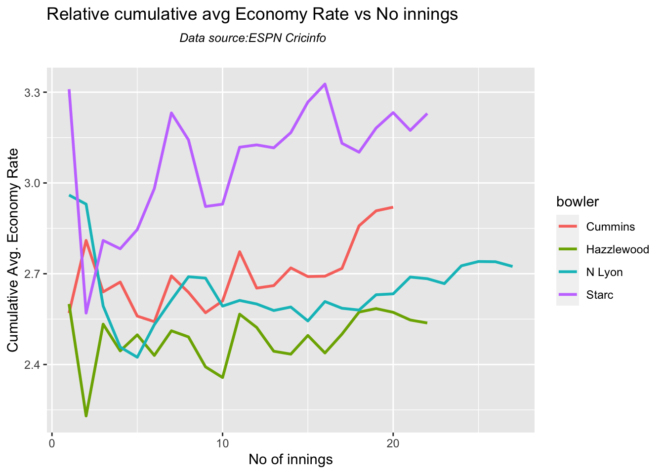
9. Analysis of Australia WTC bowlers from Jan 2016 – May 2023 against India

9a Relative cumulative average wickets of bowlers in career

Against India Lyon, Cummins and Hazzlewood have performed well

frames <- list("cumminsTestInd.csv","starcTestInd.csv","hazzlewoodTestInd.csv","lyonTestInd.csv")
names <- list("Cummins","Starc","Hazzlewood","N Lyon")
relativeBowlerCumulativeAvgWickets(frames,names)

9b Relative cumulative average economy rate of bowlers

Hazzlewood, Lyon have a good economy rate against India

frames <- list("cumminsTestInd.csv","starcTestInd.csv","hazzlewoodTestInd.csv","lyonTestInd.csv")
names <- list("Cummins","Starc","Hazzlewood","N Lyon")
relativeBowlerCumulativeAvgEconRate(frames,names)

10 Analysis of teams – India, Australia

#The data for India & Australia teams were obtained with the following calls

#indiaTest <-getTeamDataHomeAway(dir=".",teamView="bat",matchType="Test",file="indiaTest.csv",save=TRUE,teamName="India")
#australiaTest <- getTeamDataHomeAway(matchType="Test",file="australiaTest.csv",save=TRUE,teamName="Australia")

10a. Win-loss of India against all oppositions in Test cricket

Against Australia India has won 17 times, lost 60 and drawn 22 in Australia. At home India won 42, tied 2, lost 28 and drawn 24

teamWinLossStatusVsOpposition("indiaTest.csv",teamName="India",opposition=c("all"),homeOrAway=c("all"),matchType="Test",plot=TRUE)

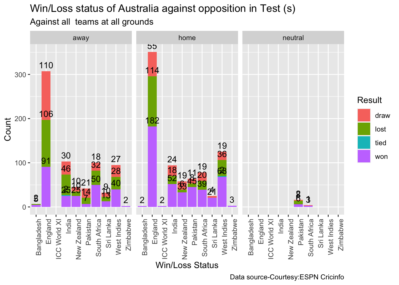
10b. Win-loss of Australia against all oppositions in Test cricket

teamWinLossStatusVsOpposition("australiaTest.csv",teamName="Australia",opposition=c("all"),homeOrAway=c("all"),matchType="Test",plot=TRUE)

10c. Win-loss of India against Australia in Test cricket

Against Australia India has won 17 times, lost 60 and drawn 22 in Australia. At home India won 42, tied 2, lost 28 and drawn 24

teamWinLossStatusVsOpposition("indiaTest.csv",teamName="India",opposition=c("Australia"),homeOrAway=c("all"),matchType="Test",plot=TRUE)

10d. Win-loss of India at all away venues

At the Oval where WTC is going to be held India has won 4, lost 10 and drawn 10.

teamWinLossStatusAtGrounds("indiaTest.csv",teamName="India",opposition=c("all"),homeOrAway=c("away"),matchType="Test",plot=TRUE)

10d. Timeline of win-loss of India against Australia in Test cricket

plotTimelineofWinsLosses("indiaTest.csv",team="India",opposition=c("Australia"),
                         homeOrAway=c("away","neutral"), startDate="2016-01-01",endDate="2023-05-01")

11. Conclusion

The above analysis performs various analysis of India and Australia in home and away matches. While we know the performance of the player at India or Australia, we cannot judge how the match will progress in the neutral, swinging conditions of the Oval. Let us hope for a good match!

Feel free to try out your own analysis with cricketr. Have fun with cricketr!!

Also see

To see all posts click Index of posts

GooglyPlusPlus: Computing T20 player’s Win Probability Contribution

In this post, I compute each batsman’s or bowler’s Win Probability Contribution (WPC) in a T20 match. This metric captures by how much the player (batsman or bowler) changed/impacted the Win Probability of the T20 match. For this computation I use my machine learning models, I had created earlier, which predicts the ball-by-ball win probability as the T20 match progresses through the 2 innings of the match.

In the picture snippet below, you can see how the win probability changes ball-by-ball for each batsman for a T20 match between CSK vs LSG- 31 Mar 2022

In my previous posts I had created several Machine Learning models. In order to compute the player’s Win Probability contribution in this post, I have used the following ML models

Logistic Regression model – glmnet : accuracy – 0.728 and roc_auc – 0.81 – Boosting Win Probability accuracy with player embeddings
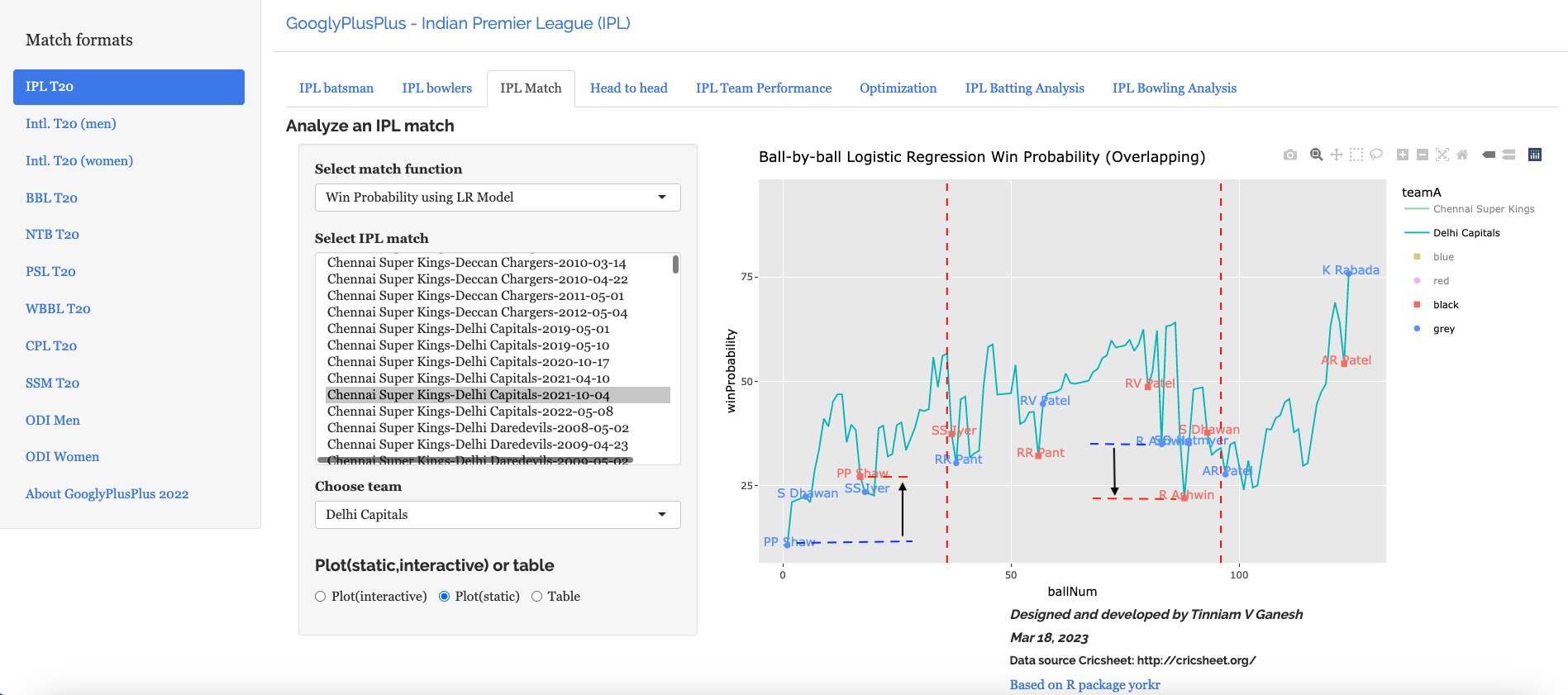
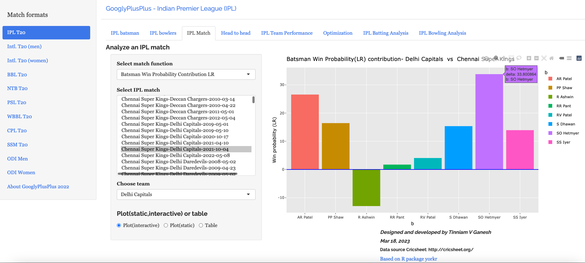
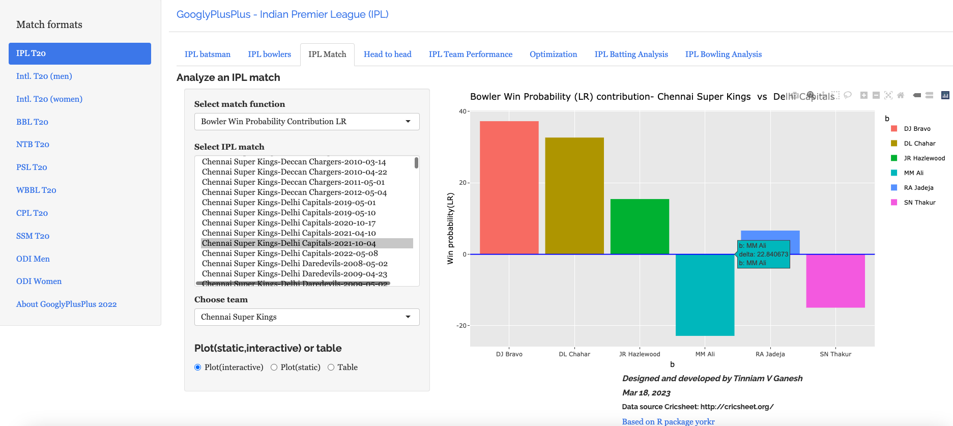
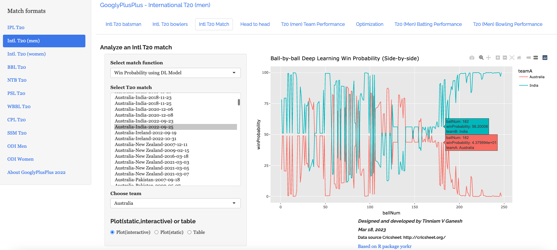
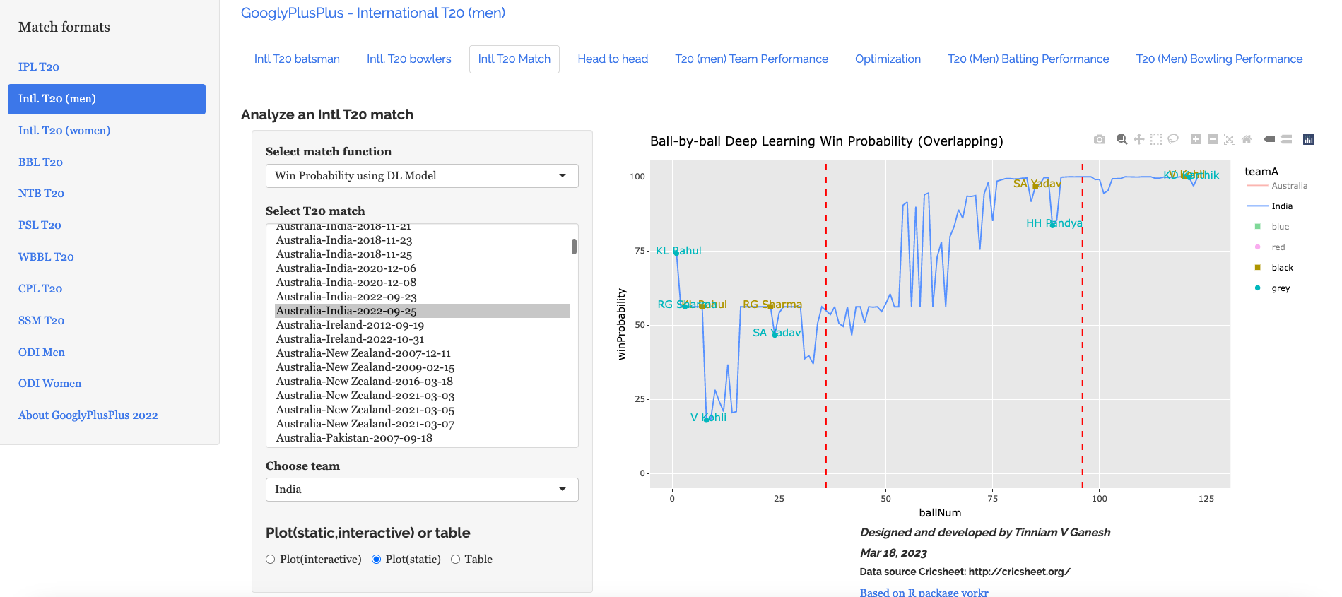
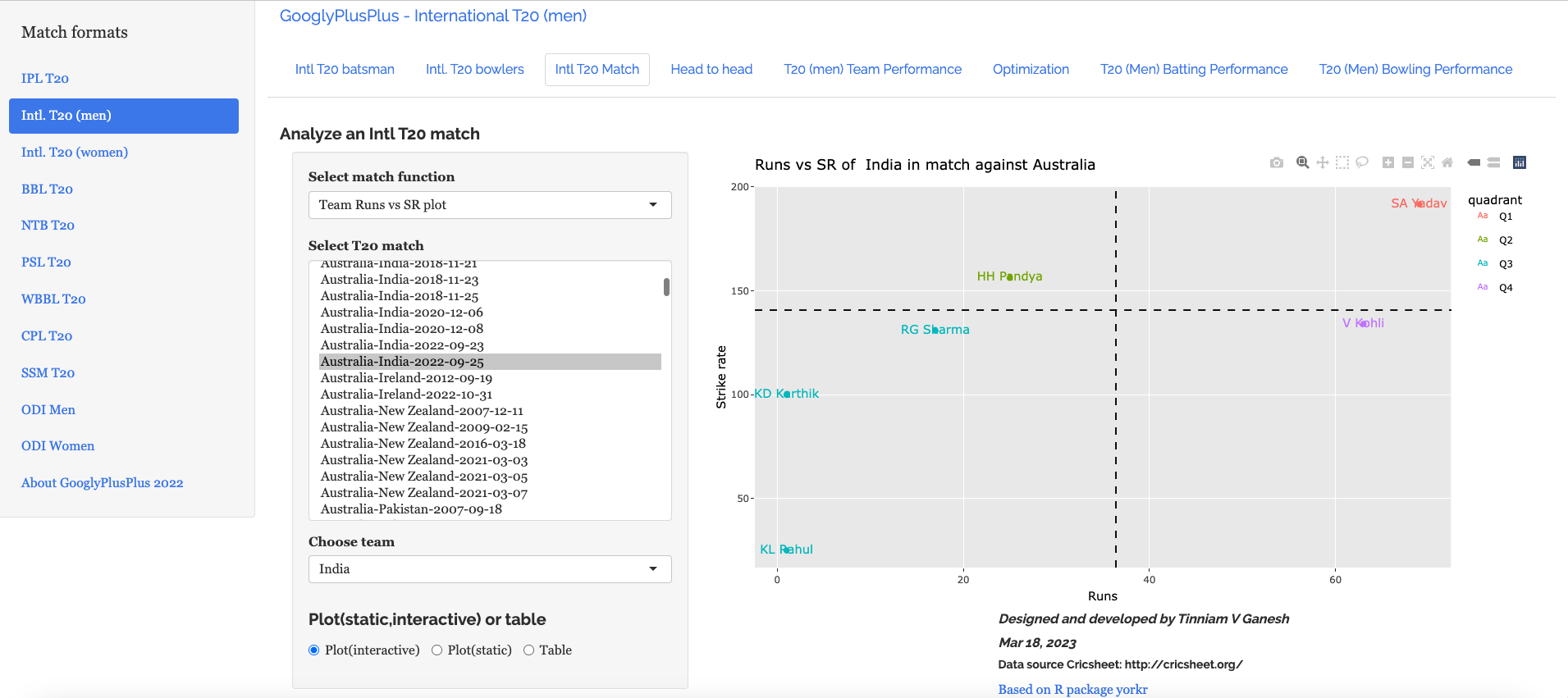
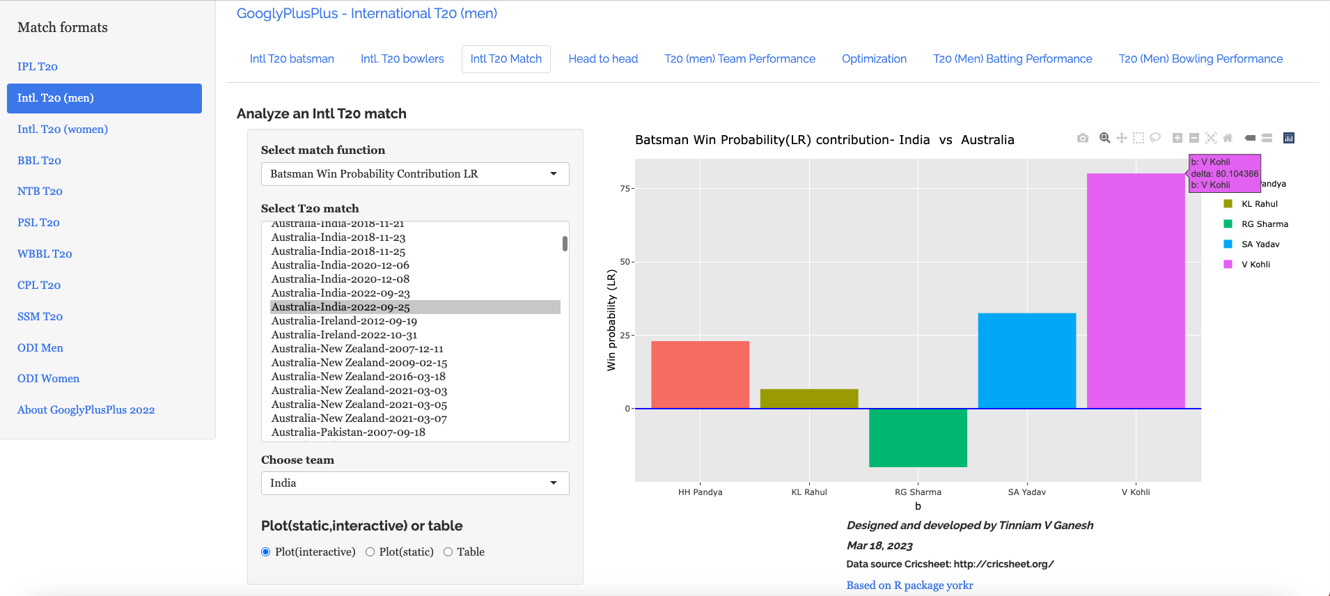
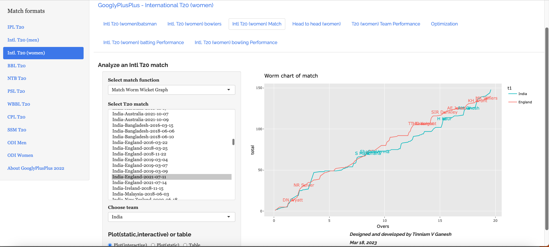
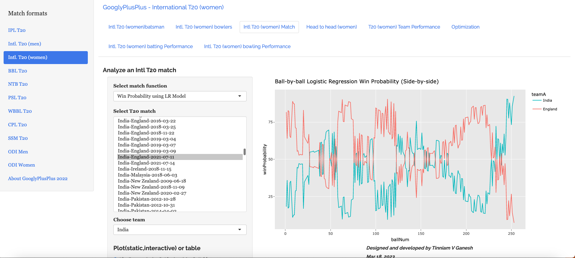
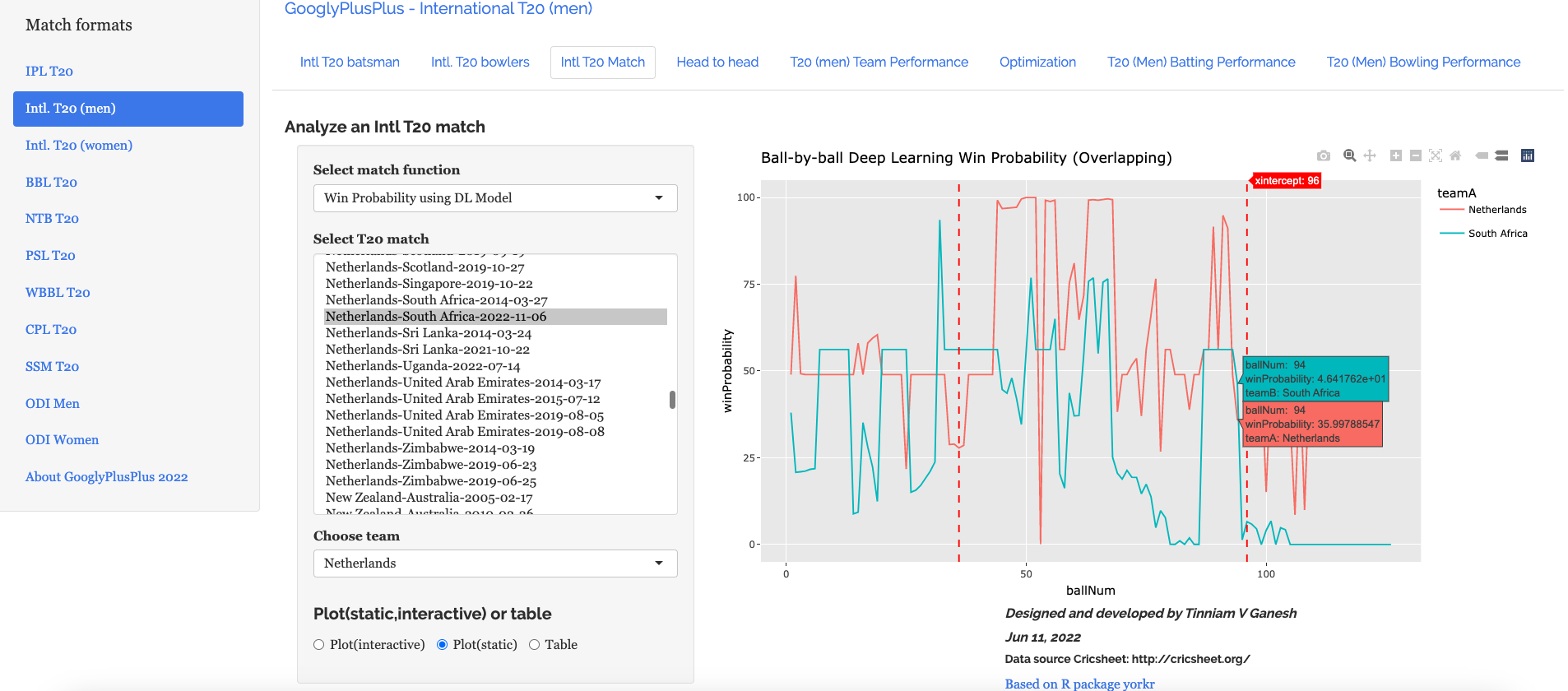
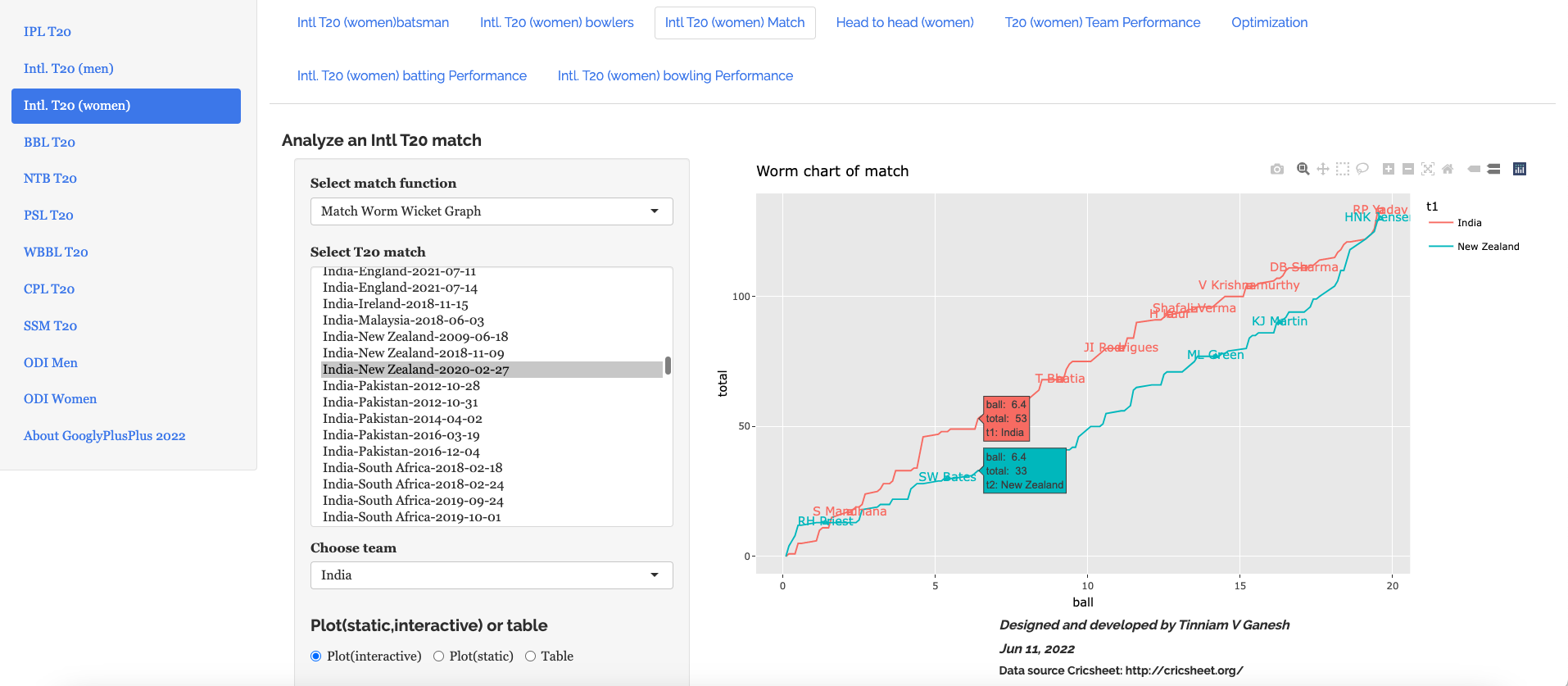
Deep Learning model – DL – accuracy – 0.8639 and roc_auc – 0.946 – GooglyPlusPlus: Win Probability using Deep Learning and player embeddings

The batsman’s or bowler’s win probability contribution changes ball-by=ball. The player’s contribution is calculated as the difference in win probability when the batsman faces the 1st ball in his innings and the last ball either when is out or the innings comes to an end. If the difference is +ve the the player has had a positive impact, and likewise for negative contribution. Similarly, for a bowler, it is the win probability when he/she comes into bowl till, the last delivery he/she bowls

Note: The Win Probability Contribution does not have any relation to the how much runs or at what strike rate the batsman scored the runs. Rather the model computes different win probability for each player, based on his/her embedding, the ball in the innings and six other feature vectors like runs, run rate, runsMomentum etc. These values change for every ball as seen in the table above. Also, this is not continuous. The 2 ML models determine the Win Probability for a specific player, ball and the context in the match.

This metric is similar to Win Probability Added (WPA) used in Sabermetrics for baseball. Here is the definition of WPA from Fangraphs “Win Probability Added (WPA) captures the change in Win Expectancy from one plate appearance to the next and credits or debits the player based on how much their action increased their team’s odds of winning.” This article in Fangraphs explains in detail how this computation is done.

In this post I have added 4 new function to my R package yorkr.

batsmanWinProbLR – batsman’s win probability contribution based on glmnet (Logistic Regression)
bowlerWinProbLR – bowler’s win probability contribution based on glmnet (Logistic Regression)
batsmanWinProbDL – batsman’s win probability contribution based on Deep Learning Model
bowlerWinProbDL – bowlerWinProbLR – bowler’s win probability contribution based on Deep Learning

Hence there are 4 additional features in GooglyPlusPlus based on the above 4 functions. In addition I have also updated

-winProbLR (overLap) function to include the names of batsman when they come to bat and when they get out or the innings comes to an end, based on Logistic Regression

-winProbDL(overLap) function to include the names of batsman when they come to bat and when they get out based on Deep Learning

Hence there are 6 new features in this version of GooglyPlusPlus.

Note: All these new 6 features are available for all 9 formats of T20 in GooglyPlusPlus namely

a) IPL b) BBL c) NTB d) PSL e) Intl, T20 (men) f) Intl. T20 (women) g) WBB h) CSL i) SSM

Check out the latest version of GooglyPlusPlus at gpp2023-2

Note: The data for GooglyPlusPlus comes from Cricsheet and the Shiny app is based on my R package yorkr

A) Chennai SuperKings vs Delhi Capitals – 04 Oct 2021

To understand Win Probability Contribution better let us look at Chennai Super Kings vs Delhi Capitals match on 04 Oct 2021

This was closely fought match with fortunes swinging wildly. If we take a look at the Worm wicket chart of this match

a) Worm Wicket chart – CSK vs DC – 04 Oct 2021

Delhi Capitals finally win the match

b) Win Probability Logistic Regression (side-by-side) – CSK vs DC – 4 Oct 2021

Plotting how win probability changes over the course of the match using Logistic Regression Model

In this match Delhi Capitals won. The batting scorecard of Delhi Capitals

c) Batting Scorecard of Delhi Capitals – CSK vs DC – 4 Oct 2021

d) Win Probability Logistic Regression (Overlapping) – CSK vs DC – 4 Oct 2021

The Win Probability LR (overlapping) shows the probability function of both teams superimposed over one another. The plot includes when a batsman came into to play and when he got out. This is for both teams. This looks a little noisy, but there is a way to selectively display the change in Win Probability for each team. This can be done , by clicking the 3 arrows (orange or blue) from top to bottom. First double-click the team CSK or DC, then click the next 2 items (blue,red or black,grey) Sorry the legends don’t match the colors! 😦

Below we can see how the win probability changed for Delhi Capitals during their innings, as batsmen came into to play. See below

e) Batsman Win Probability contribution:DC – CSK vs DC – 4 Oct 2021

Computing the individual batsman’s Win Contribution and plotting we have. Hetmeyer has a higher Win Probability contribution than Shikhar Dhawan depsite scoring fewer runs

f) Bowler’s Win Probability contribution :CSK – CSK vs DC – 4 Oct 2021

We can also check the Win Probability of the bowlers. So for e.g the CSK bowlers and which bowlers had the most impact. Moeen Ali has the least impact in this match

B) Intl. T20 (men) Australia vs India – 25 Sep 2022

a) Worm wicket chart – Australia vs India – 25 Sep 2022

This was another close match in which India won with the penultimate ball

b) Win Probability based on Deep Learning model (side-by-side) – Australia vs India – 25 Sep 2022

c) Win Probability based on Deep Learning model (overlapping) – Australia vs India – 25 Sep 2022

The plot below shows how the Win Probability of the teams varied across the 20 overs. The 2 Win Probability distributions are superimposed over each other

d) Batsman Win Probability Contribution : India – Australia vs India – 25 Sep 2022

Selectively choosing the India Win Probability plot by double-clicking legend ‘India’ on the right , followed by single click of black, grey legend we have

We see that Kohli, Suryakumar Yadav have good contribution to the Win Probability

e) Plotting the Runs vs Strike Rate:India – Australia vs India – 25 Sep 2022

f) Batsman’s Win Probability Contribution- Australia vs India – 25 Sep 2022

Finally plotting the Batsman’s Win Probability Contribution

Interestingly, Kohli has a greater Win Probability Contribution than SKY, though SKY scored more runs at a better strike rate. As mentioned above, the Win Probability is context dependent and also depends on past performances of the player (batsman, bowler)

Finally let us look at

C) India vs England Intll T20 Women (11 July 2021)

a) Worm wicket chart – India vs England Intl. T20 Women (11 July 2021)

India won this T20 match by 8 runs

b) Win Probability using the Logistic Regression Model – India vs England Intl. T20 Women (11 July 2021)

c) Win Probability with the DL model – India vs England Intl. T20 Women (11 July 2021)

d) Bowler Win Probability Contribution with the LR model – India vs England Intl. T20 Women (11 July 2021)

e) Bowler Win Contribution with the DL model – India vs England Intl. T20 Women (11 July 2021)

Go ahead and try out the latest version of GooglyPlusPlus

Also see my other posts

To see all posts click Index of posts

GooglyPlusPlus: Win Probability using Deep Learning and player embeddings

In my last post ‘GooglyPlusPlus now with Win Probability Analysis for all T20 matches‘ I had discussed the performance of my ML models, created with and without player embeddings, in computing the Win Probability of T20 matches. With batsman & bowler embeddings I got much better performance than without the embeddings

glmnet – Accuracy – 0.73
Random Forest (RF) – Accuracy – 0.92

While the Random Forest gave excellent accuracy, it was bulky and also took an unusually long time to predict the Win Probability of a single T20 match. The above 2 ML models were built using R’s Tidymodels. glmnet was fast, but I wanted to see if I could create a ML model that was better, lighter and faster. I had initially tried to use Tensorflow, Keras in Python but then abandoned it, since I did not know how to port the Deep Learning model to R and use in my app GooglyPlusPlus.

But later, since I was stuck with a bulky Random Forest model, I decided to again explore options for saving the Keras Deep Learning model and loading it in R. I found out that saving the model as .h5, we can load it in R and use it for predictions. Hence, I rebuilt a Deep Learning model using Keras, Python with player embeddings and I got excellent performance. The DL model was light and had an accuracy 0.8639 with an ROC_AUC of 0.964 which was great!

GooglyPlusPlus uses data from Cricsheet and is based on my R package yorkr

You can try out this latest version of GooglyPlusPlus at gpp2023-1

Here are the steps

A. Build a Keras Deep Learning model

a. Import necessary packages

import pandas as pd
import numpy as np
from zipfile import ZipFile
import tensorflow as tf
from tensorflow import keras
from tensorflow.keras import layers
from tensorflow.keras import regularizers
from pathlib import Path
import matplotlib.pyplot as plt

b, Upload the data of all 9 T20 leagues (BBL, CPL, IPL, T20 (men) , T20(women), NTB, CPL, SSM, WBB)

# Read all T20 leagues 
df1=pd.read_csv('t20.csv')
print("Shape of dataframe=",df1.shape)

# Create training and test data set
train_dataset = df1.sample(frac=0.8,random_state=0)
test_dataset = df1.drop(train_dataset.index)
train_dataset1 = train_dataset[['batsmanIdx','bowlerIdx','ballNum','ballsRemaining','runs','runRate','numWickets','runsMomentum','perfIndex']]
test_dataset1 = test_dataset[['batsmanIdx','bowlerIdx','ballNum','ballsRemaining','runs','runRate','numWickets','runsMomentum','perfIndex']]
train_dataset1

# Set the target data
train_labels = train_dataset.pop('isWinner')
test_labels = test_dataset.pop('isWinner')
train_dataset1

a=train_dataset1.describe()
stats=a.transpose
a

c. Create a Deep Learning ML model using batsman & bowler embeddings

import pandas as pd
import numpy as np
from keras.layers import Input, Embedding, Flatten, Dense
from keras.models import Model
from keras.layers import Input, Embedding, Flatten, Dense, Reshape, Concatenate, Dropout
from keras.models import Model

# Set seed
tf.random.set_seed(432)

# create input layers for each of the predictors
batsmanIdx_input = Input(shape=(1,), name='batsmanIdx')
bowlerIdx_input = Input(shape=(1,), name='bowlerIdx')
ballNum_input = Input(shape=(1,), name='ballNum')
ballsRemaining_input = Input(shape=(1,), name='ballsRemaining')
runs_input = Input(shape=(1,), name='runs')
runRate_input = Input(shape=(1,), name='runRate')
numWickets_input = Input(shape=(1,), name='numWickets')
runsMomentum_input = Input(shape=(1,), name='runsMomentum')
perfIndex_input = Input(shape=(1,), name='perfIndex')

# Set the embedding size as the 4th root of unique batsmen, bowlers
no_of_unique_batman=len(df1["batsmanIdx"].unique()) 
no_of_unique_bowler=len(df1["bowlerIdx"].unique()) 
embedding_size_bat = no_of_unique_batman ** (1/4)
embedding_size_bwl = no_of_unique_bowler ** (1/4)


# create embedding layer for the categorical predictor
batsmanIdx_embedding = Embedding(input_dim=no_of_unique_batman+1, output_dim=16,input_length=1)(batsmanIdx_input)
batsmanIdx_flatten = Flatten()(batsmanIdx_embedding)
bowlerIdx_embedding = Embedding(input_dim=no_of_unique_bowler+1, output_dim=16,input_length=1)(bowlerIdx_input)
bowlerIdx_flatten = Flatten()(bowlerIdx_embedding)

# concatenate all the predictors
x = keras.layers.concatenate([batsmanIdx_flatten,bowlerIdx_flatten, ballNum_input, ballsRemaining_input, runs_input, runRate_input, numWickets_input, runsMomentum_input, perfIndex_input])

# add hidden layers
# Use dropouts for regularisation
x = Dense(64, activation='relu')(x)
x = Dropout(0.1)(x)
x = Dense(32, activation='relu')(x)
x = Dropout(0.1)(x)
x = Dense(16, activation='relu')(x)
x = Dropout(0.1)(x)
x = Dense(8, activation='relu')(x)
x = Dropout(0.1)(x)

# add output layer
output = Dense(1, activation='sigmoid', name='output')(x)
print(output.shape)

# create a DL model
model = Model(inputs=[batsmanIdx_input,bowlerIdx_input, ballNum_input, ballsRemaining_input, runs_input, runRate_input, numWickets_input, runsMomentum_input, perfIndex_input], outputs=output)
model.summary()

# compile model
optimizer=keras.optimizers.Adam(learning_rate=.01, beta_1=0.9, beta_2=0.999, epsilon=1e-07, decay=0.0, amsgrad=True)

model.compile(optimizer=optimizer, loss='binary_crossentropy', metrics=['accuracy'])

# train the model
history=model.fit([train_dataset1['batsmanIdx'],train_dataset1['bowlerIdx'],train_dataset1['ballNum'],train_dataset1['ballsRemaining'],train_dataset1['runs'],
           train_dataset1['runRate'],train_dataset1['numWickets'],train_dataset1['runsMomentum'],train_dataset1['perfIndex']], train_labels, epochs=40, batch_size=1024,
          validation_data = ([test_dataset1['batsmanIdx'],test_dataset1['bowlerIdx'],test_dataset1['ballNum'],test_dataset1['ballsRemaining'],test_dataset1['runs'],
           test_dataset1['runRate'],test_dataset1['numWickets'],test_dataset1['runsMomentum'],test_dataset1['perfIndex']],test_labels), verbose=1)

plt.plot(history.history["loss"])
plt.plot(history.history["val_loss"])
plt.title("model loss")
plt.ylabel("loss")
plt.xlabel("epoch")
plt.legend(["train", "test"], loc="upper left")
plt.show()

Model: "model_5"
__________________________________________________________________________________________________
 Layer (type)                   Output Shape         Param #     Connected to                     
==================================================================================================
 batsmanIdx (InputLayer)        [(None, 1)]          0           []                               
                                                                                                  
 bowlerIdx (InputLayer)         [(None, 1)]          0           []                               
                                                                                                  
 embedding_10 (Embedding)       (None, 1, 16)        75888       ['batsmanIdx[0][0]']             
                                                                                                  
 embedding_11 (Embedding)       (None, 1, 16)        55808       ['bowlerIdx[0][0]']              
                                                                                                  
 flatten_10 (Flatten)           (None, 16)           0           ['embedding_10[0][0]']           
                                                                                                  
 flatten_11 (Flatten)           (None, 16)           0           ['embedding_11[0][0]']           
                                                                                                  
 ballNum (InputLayer)           [(None, 1)]          0           []                               
                                                                                                  
 ballsRemaining (InputLayer)    [(None, 1)]          0           []                               
                                                                                                  
 runs (InputLayer)              [(None, 1)]          0           []                               
                                                                                                  
 runRate (InputLayer)           [(None, 1)]          0           []                               
                                                                                                  
 numWickets (InputLayer)        [(None, 1)]          0           []                               
                                                                                                  
 runsMomentum (InputLayer)      [(None, 1)]          0           []                               
                                                                                                  
 perfIndex (InputLayer)         [(None, 1)]          0           []                               
                                                                                                  
 concatenate_5 (Concatenate)    (None, 39)           0           ['flatten_10[0][0]',             
                                                                  'flatten_11[0][0]',             
                                                                  'ballNum[0][0]',                
                                                                  'ballsRemaining[0][0]',         
                                                                  'runs[0][0]',                   
                                                                  'runRate[0][0]',                
                                                                  'numWickets[0][0]',             
                                                                  'runsMomentum[0][0]',           
                                                                  'perfIndex[0][0]']              
                                                                                                  
 dense_19 (Dense)               (None, 64)           2560        ['concatenate_5[0][0]']          
                                                                                                  
 dropout_19 (Dropout)           (None, 64)           0           ['dense_19[0][0]']               
                                                                                                  
 dense_20 (Dense)               (None, 32)           2080        ['dropout_19[0][0]']             
                                                                                                  
 dropout_20 (Dropout)           (None, 32)           0           ['dense_20[0][0]']               
                                                                                                  
 dense_21 (Dense)               (None, 16)           528         ['dropout_20[0][0]']             
                                                                                                  
 dropout_21 (Dropout)           (None, 16)           0           ['dense_21[0][0]']               
                                                                                                  
 dense_22 (Dense)               (None, 8)            136         ['dropout_21[0][0]']             
                                                                                                  
 dropout_22 (Dropout)           (None, 8)            0           ['dense_22[0][0]']               
                                                                                                  
 output (Dense)                 (None, 1)            9           ['dropout_22[0][0]']             
                                                                                                  
==================================================================================================
Total params: 137,009
Trainable params: 137,009
Non-trainable params: 0
__________________________________________________________________________________________________
Epoch 1/40
937/937 [==============================] - 11s 10ms/step - loss: 0.5683 - accuracy: 0.6968 - val_loss: 0.4480 - val_accuracy: 0.7708
Epoch 2/40
937/937 [==============================] - 9s 10ms/step - loss: 0.4477 - accuracy: 0.7721 - val_loss: 0.4305 - val_accuracy: 0.7833
Epoch 3/40
937/937 [==============================] - 9s 10ms/step - loss: 0.4229 - accuracy: 0.7832 - val_loss: 0.3984 - val_accuracy: 0.7936
...
...
937/937 [==============================] - 10s 10ms/step - loss: 0.2909 - accuracy: 0.8627 - val_loss: 0.2943 - val_accuracy: 0.8613
Epoch 38/40
937/937 [==============================] - 10s 10ms/step - loss: 0.2892 - accuracy: 0.8633 - val_loss: 0.2933 - val_accuracy: 0.8621
Epoch 39/40
937/937 [==============================] - 10s 10ms/step - loss: 0.2889 - accuracy: 0.8638 - val_loss: 0.2941 - val_accuracy: 0.8620
Epoch 40/40
937/937 [==============================] - 10s 11ms/step - loss: 0.2886 - accuracy: 0.8639 - val_loss: 0.2929 - val_accuracy: 0.8621

d. Compute and plot the ROC-AUC for the above model

from sklearn.metrics import roc_curve

# Select a random sample set
tf.random.set_seed(59)
train = df1.sample(frac=0.9,random_state=0)
test = df1.drop(train_dataset.index)
test_dataset1 = test[['batsmanIdx','bowlerIdx','ballNum','ballsRemaining','runs','runRate','numWickets','runsMomentum','perfIndex']]
test_labels = test.pop('isWinner')

# Compute the predicted values
y_pred_keras = model.predict([test_dataset1['batsmanIdx'],test_dataset1['bowlerIdx'],test_dataset1['ballNum'],test_dataset1['ballsRemaining'],test_dataset1['runs'],
           test_dataset1['runRate'],test_dataset1['numWickets'],test_dataset1['runsMomentum'],test_dataset1['perfIndex']]).ravel()

# Compute TPR & FPR
fpr_keras, tpr_keras, thresholds_keras = roc_curve(test_labels, y_pred_keras)

fpr_keras, tpr_keras, thresholds_keras = roc_curve(test_labels, y_pred_keras)
from sklearn.metrics import auc

# Plot the Area Under the Curve (AUC)
auc_keras = auc(fpr_keras, tpr_keras)
plt.figure(1)
plt.plot([0, 1], [0, 1], 'k--')
plt.plot(fpr_keras, tpr_keras, label='Keras (area = {:.3f})'.format(auc_keras))
plt.xlabel('False positive rate')
plt.ylabel('True positive rate')
plt.title('ROC curve')
plt.legend(loc='best')
plt.show()

The ROC_AUC for the Deep Learning Model is 0.946 as seen below

e. Save the Keras model for use in Python

from keras.models import Model
model.save("wpDL.h5")

f. Load the model in R using rhdf5 package for use in GooglyPlusPlus

library(rhdf5)
dl_model <- load_model_hdf5('wpDL.h5')

This was a huge success for me to be able to create the Deep Learning model in Python and use it in my Shiny app GooglyPlusPlus. The Deep Learning Keras model is light-weight and extremely fast.

The Deep Learning model has now been integrated into GooglyPlusPlus. Now you can check the Win Probability using both a) glmnet (Logistic Regression with lasso regularisation) b) Keras Deep Learning model with dropouts as regularisation

In addition I have created 2 features based on Win Probability (WP)

i) Win Probability (Side-by-side – Plot(interactive) : With this functionality the 1st and 2nd innings will be side-by-side. When the 1st innings is played by team 1, the Win Probability of team 2 = 100 – WP (team1). Similarly, when the 2nd innings is being played by team 2, the Win Probability of team1 = 100 – WP (team 2)

ii) Win Probability (Overlapping) – Plot (static): With this functionality the Win Probabilities of both team1(1st innings) & team 2 (2nd innings) are displayed overlapping, so that we can see how the probabilities vary ball-by-ball.

Note: Since the same UI is used for all match functions I had to re-use the Plot(interactive) and Plot(static) radio buttons for Win Probability (Side-by-side) and Win Probability(Overlapping) respectively

Here are screenshots using both ML models with both functionality for some random matches

B) ICC T20 Men World Cup – Netherland-South Africa- 2022-11-06

i) Match Worm wicket chart

ii) Win Probability with LR (Side-by-Side- Plot(interactive))

iii) Win Probability LR (Overlapping- Plot(static))

iv) Win Probability Deep Learning (Side-by-side – Plot(interactive)

In the 213th ball of the innings South Africa was slightly ahead of Netherlands. After that they crashed and burned!

v) Win Probability Deep Learning (Overlapping – Plot (static)

It can be seen that in the 94th ball of both innings South Africa was ahead of Netherlands before the eventual slump.

C) Intl. T20 (Women) India – New Zealand – 2020 – 02 – 27

Here is an interesting match between India and New Zealand T20 Women’s teams. NZ successfully chased the India’s total in a wildly swinging fortunes. See the charts below

i) Match Worm Wicket chart

ii) Win Probability with LR (Side-by-side – Plot (interactive)

iii) Win Probability with LR (Overlapping – Plot (static)

iv) Win Probability with DL model (Side-by-side – Plot (interactive))

v) Win Probability with DL model (Overlapping – Plot (static))

The above functionality in plotting the Win Probability using LR or DL with both options (Side-by-side or Overlapping) is available for all 9 T20 leagues currently supported by GooglyPlusPlus.

Go ahead and give gpp2023-1 a try!!!

Do also check out my other posts’

To see all posts click Index of posts

Near Real-time Analytics of ICC Men’s T20 World Cup with GooglyPlusPlus

In my last post GooglyPlusPlus gets ready for ICC Men’s T20 World Cup, I had mentioned that GooglyPlusPlus was preparing for the big event the ICC Men’s T20 World cup. Now that the T20 World cup is underway, my Shiny app in R, GooglyPlusPlus ,will be generating near real-time analytics of matches completed the previous day. Besides the app can also do historical analysis of players, teams and matches.

The whole process is automated. A cron job will execute every day, in the morning, which will automatically download the matches of the previous day from Cricsheet, unzip them, start a pipeline which will transform and process the match data into necessary folders and finally upload the newly acquired data into my Shiny app. Hence, you will be able to access all the breathless, pulsating cricketing action in timeless, interactive plots and tables which will capture all aspects of Men’s T20 matches, namely batsman, bowler performance, match analysis, team-vs-team, team-vs-all teams besides ranking of batsmen & bowlers. Since the data is cumulative, all the analytics are historical and current.

Check out GooglyPlusPlus!!

The data for GooglyPlusPlus is taken from Cricsheet

Interest in cricket, has mushroomed in recent times around the world, with the addition of new formats which started with ODI, T20, T10, 100 ball and so on. There are leagues which host these matches at different levels around the world. While GooglyPlusPlus, provides near real-time analytics of Men’s T20 World cup, we can clearly envision a big data platform which ingests matches daily from multiple cricket formats, leagues around the world generating real-time and near real-time analytics which are essential these days to selection of teams at different levels through auctions. For more discussion on this see my posts

We could imagine a Data Lake, into which are ingested data from the different cricket formats, leagues through appropriate technology connectors. Once the data is ingested, we could have data pipelines, based on Azure ADF, Apache NiFi, Apache Airflow or Amazon EMR etc., to transform, process and enhance the data, generating real-time analytics on the fly. Recent formats like T20, T10 require more urgency in strategic thinking based on scoring within limited overs, or containing batsmen from going on a rampage within the set of overs, the analytics on a fly may help the coach to modify the batting or bowling lineup at points in match. In this context see my earlier post Using Linear Programming (LP) for optimizing bowling change or batting lineup in T20 cricket

All of these are not just possible, but are likely to become reality as more and more formats, leagues and cricket data proliferate around the world.

This post, focuses on generating near-real time analytics for ICC Men’s T20 World Cup using GooglyPlusPlus. Included below, is a sampling of the analytics that you can perform for analysing the matches. In addition you can do all the analysis included in my post GooglyPlusPlus gets ready for ICC Men’s T20 World Cup

Namibia-Sri Lanka-16 Oct 2022 : Match Worm graph

The opening match between Namibia vs Sri Lanka resulted in an upset. We can see this in the match worm-wicket graph below

2. Scotland vs West Indies – 17 Oct 2022: Batsmen vs Bowlers

George Munsey was the top scorer for Scotland and was instrumental in the win against WI. His performance against West Indies bowlers is shown below. Note, the charts are interactive

3. Zimbabwe vs Ireland – 17 Oct 2022 : Team Runs vs SR

Sikander Raza of Zimbabwe with 82 runs with the strike rate ~ 170

4. United Arab Emirates vs Netherlands – 16 Oct 2022: Team runs across 20 overs

UAE pipped Netherlands in the middle overs and were able to win by 1 ball and 3 wickets

5. Scotland vs Ireland – 19 Oct 2022 : Team Runs vs SR Middle overs plot

Curtis Campher snatched the game away from Scotland with his stellar performance in middle and death overs

6. UAE vs Namibia : 20 Oct 2022 : Team Wickets vs ER plot

Basoor Hameed and Zahoor Khan got 2 wickets apiece with an economy rate of ~5.00 but still they were not able to stop UAE from stealing a win

7. Overall Runs vs SR in T20 World Cup 2022

It is too early to rank the players, nevertheless in the current T20 World Cup, MP O’Dowd (Netherlands), BKG Mendis (Sri Lanka) and JN Frylinck(Namibia) are the top 3 batsmen with good runs and Strike Rate

8. Overall Wickets over ER in T20 World Cup 2022

The top 3 bowlers so far in T20 World Cup 2022 are a) BFW de Leede (Netherlands) b) PWH De Silva (Sri Lanka) c) KP Meiyappan (UAE) with a total of 7,7, and 6 wickets respectively

Note: Besides the match analysis GooglyPlusPlus also provides detailed analysis of batsmen, bowlers, matches as above, team-vs-team, team-vs-all teams, ranking of batsmen & bowlers etc. For more details see my post GooglyPlusPlus gets ready for ICC Men’s T20 World Cup

Do visit GooglyPlusPlus everyday to check out the cricketing actions of matches gone by. You can also follow me on twitter @tvganesh_85 for daily highlights.

GooglyPlusPlus gets ready for ICC Men’s T20 World Cup

It is time!! So last weekend, I turned the wheels, moved the levers and listened to the hiss of steam, as I cranked up my Shiny app GooglyPlusPlus. The ICC Men’s T20 World Cup is just around the corner, and it was time to prepare for this event. This latest GooglyPlusPlus is current with the latest Intl. men’s T20 match data, give or take a few. GooglyPlusPlus can analyze batsmen, bowlers, matches, team-vs-team, team-vs-all teams, besides also ranking batsmen, bowlers and plot performances in Powerplay, middle and death overs.

In this post, I include a quick refresher of some of features of my app GooglyPlusPlus. Note: This is a random sampling of the functions available. There are more than 120+ features available in the app.

Check out your favourite players and your country’s team with GooglyPlusPlus

Note 1: All charts are interactive

Note 2: You can choose a date range for your analysis

Note 3: The data for this app is taken from Cricsheet

T20 Batsman tab

This tab includes functions pertaining to individual batsmen. Functions include Runs vs Deliveries, moving average runs, cumulative average run, cumulative average strike rate, runs against opposition, runs at venue etc.

For e.g.

a) Suryakumar Yadav’s (India) cumulative strike rate

b) Mohammed Rizwan’s (Pakistan) performance against opposition

2. T20 Bowler’s Tab

The bowlers tab has functions for computing mean economy rate, moving average wickets, cumulative average wicks, cumulative economy rate, bowlers performance against opposition, bowlers performance in venue, predict wickets and others

A random function is shown below

a) Predict wickets for Wanindu Hasaranga of Sri Lanka

3. T20 Match tab

The match tab has functions that can compute match batting & bowling scorecard, batting partnerships, batsmen performance vs bowlers, bowler’s wicket kind, bowler’s wicket match, match worm graph, match worm wicket graph, team runs across 20 overs, team wickets in 20 overs, teams runs or wickets in powerplay, middle and death overs

Here are a couple of functions from this tab

a) Afghanistan vs Ireland – 2022-08-15

b) Australia vs Sri Lanka – 2019-11-01 – Runs across 20 overs

4. T20 Head-to-head tab

This tab provides the analysis of all combination of T20 teams (countries) in different aspects. This tab can compute the overall batting, bowling scorecard in all matches between 2 countries, batsmen partnerships, performances against bowlers, bowlers vs batsmen, runs, strike rate, wickets, economy rate across 20 overs, runs vs SR plot and wicket vs ER plot in all matches between team and so on. Here are a couple of examples from this tab

a) Bangladesh vs West Indies – Batting scorecard from 2019-01-01 to 2022-07-07

b) Wickets vs ER plot – England vs New Zealand – 2019-01-01 to 2021-11-10

5. T20 Team performance overall tab

This tab provides detailed analysis of the team’s performance against all other teams. As in the previous tab there are functions to compute the overall batting, bowling scorecard of a team against all other teams for any specific interval of time. This can help in picking out the most consistent batsmen, bowlers. Besides there are functions to compute overall batting partnerships, bowler vs batsmen, runs, wickets across 20 overs, run vs SR and wickets vs ER etc.

a) Batsmen vs Bowlers (Rank 1- V Kohli 2019-01-01 to 2022-09-25)

b) team Runs vs SR in Death overs (India) (2019-01-01 to 2022-09-25)

6) Optimisation tab

In the optimisation tab we can check the performance of a specific batsmen against specific bowlers or bowlers against batsmen

a) Batsmen vs Bowlers

b) Bowlers vs batsmen

7) T20 Batting Performance tab

This tab performs various analytics like ranking batsmen based on Run over SR and SR over Runs. Also you can plot overall Runs vs SR, and more specifically Runs vs SR in Powerplay, Middle and Death overs. All of this can be done for a specific date range. Here are some examples. The data includes all of T20 (all countries all matches)

a) Rank batsmen (Runs over SR, minimum matches played=33, date range=2019-01-01 to 2022-09-27)

The top 3 batsmen are Mohamen Rizwan, V Kohli and Babar Azam

b) Overall runs vs SR plot (2019-01-01 to 2022-09-27)

c) Overall Runs vs SR in Powerplay (all teams- 2019-01-01-2022-09-27)

This plot will be crowded. However, we can zoom into an area of interest. The controls for interacting with the plot are in the top of the plot as shown

Zooming in and panning to the area we can see the best performers in powerplay are as below

8) T20 Bowling Performance tab

This tab computes and ranks bowlers on Wickets over Economy and Economy rate over wickets. We can also compute and plot the Wickets vs ER in all matches , besides the Wickets vs ER in powerplay, middle and death overs with data from all countries

a) Rank Bowlers (Wickets over ER, minimum matches=28, 2019-01-01 to 2022-09-27)

b) Wickets vs ER plot

S Lamichhane (NEP), Hasaranga (SL) and Shamsi (SA) are excellent bowlers with high wickets and low ER as seen in the plot below

c) Wickets vs ER in death overs (2019-01-01 to 2022-09-27, min matches=24)

Zooming in and panning we see the best performers in death overs are MR Adair (IRE), Haris Rauf(PAK) and Chris Jordan (ENG)

With the excitement building up, it is time you checked out how your country will perform and the players who will do well.

Go ahead give GooglyPlusPlus a spin !!!

Also see

To see all posts click Index of posts

Then, Now(IPL 2022), Beyond : Insights from GooglyPlusPlus

IPL 2022 has just concluded and yet again, it is has thrown a lot of promising and potential youngsters in its wake, while established players have fallen! With IPL 2022, we realise that “Sceptre and Crown must tumble down” and that ‘the glories‘ of form and class like everything else are “shadows not substantial things” (Death the Leveller by James Shirley).

So King Kohli had to kneel, and hitman’ himself got hit. Rishabh Pant, Jadeja also had a poor season. On the contrary there were several youngsters who shone like Abhishek Sharma, Tilak Verma, Umran Malik or a Mohsin Khan

This post is about my potential T20 Indian players for the World Cup 2022 and beyond.

The post below includes my own analysis and thoughts. Feel free to try out my Shiny app GooglyPlusPlus and draw your own conclusions.

You can also view the analyais as a youtube video at Insights from GooglyPlusPlus

How often we hear that data by itself is useless, unless we can draw insights from it? This is a prevailing theme in the corporate world and everybody uses all sorts of tools to analyse and subsequently draw insights. Data analysis can be done in many ways as data can be sliced, diced, chopped in a zillion ways. There are many facets and perspectives to analysing data. Creating insights is easy, but arriving at actionable insights is anything but. So, the problem of selecting the best 11 is difficult as there are so many ways to look at the analysis. My Shiny app GooglyPlusPlus based on my R package yorkr can analyse data in several ways namely

Batsman analysis
Bowler analysis
Match analysis
Team vs team analysis
Team vs all teams analysis
Batsman vs bowler and vice versa
Analysis of in 3,4,5 in power play, middle and death overs

GooglyPlusPlus uses my R package yorkr which has ~ 160 functions some which have several options. So, we can say roughly there are ~500 different ways that analysis can be done or in other words we can gather almost roughly 500+ different insights, not to mention that there are so many combinations of head-on matches and one-vs-all matches.

So generating insights or different ways of analysis data alone is not enough. The question is whether we can get a consolidated view from the different insights. In this post, I try to identify the best contenders for the Indian T20 team. This is far more difficult than it looks. Do you select players on past historical performance or do you choose from the newer crop of players, who have excelled in the recent IPL season. I think this boils down the typical situation in any domain. In engineering, we have tradeoffs – processing power vs memory tradeoff, throughput vs latency tradeoff or in the financial domain it is cost vs benefit or risk vs reward tradeoff. For team selection, the quandary is, whether to choose seasoned players with good historical performance but a poor performances in recent times or go with youngsters who have played with great courage and flair in this latest episode of IPL 2022. Hence there is a tradeoff between reliable but below average performance or risky but superlative performances of new players.

For this I base my potential list from

Then (past history of batsmen & bowlers) – I have chosen the performance of batsmen and bowlers in the last 3 years. With we can arrive at those who have had reasonably reliable performance for the last 3 years
Now (IPL 2022) – Performance in the current season IPL 2022

A. Then (Jan 2020 – May 2022) – Batsmen analysis

In this section I analyse the performances of batsmen and bowlers from Jan 2022 – May 2022. This is done based on ranking, and plots of Runs vs Strike Rate in Power Play, Middle and Death overs

Also I analyse bowlers based on the overall rank from Jan 2022- May 2022. Further more analysis is done on Wickets vs Economy Rate overall and in Power Play, Middle and Death overs

a. Ranks of batsmen (Runs over Strike Rate) : Jan 2020 – May 2022

The top batsmen consistency wise

[KL Rahul, Shikhar Dhawan, Ruturaj Gaikwad, Ishan Kishan, Shubman Gill, Suryakumar Yadav, Sanju Samson, Mayank Agarwal, Prithvi Shaw, Devdutt Padikkal, Nitish Rana, Virat Kohli, Shreyas Iyer, Ambati Rayadu, Rahul Tripathi, Rishabh Pant, Rohit Sharma, Hardik Pandya]

b. Ranks of batsmen (Strike Rate over Runs) : Jan 2020 – May 2022

The most consistent players from the Strike Rate perspective are

The batsmen with best Strike Rate in the last 3 years are

[Dinesh Karthik, Prithvi Shaw, Hardik Pandya, Rishabh Pant, Sanju Samson, Rahul Tripathi, Suryakumar Yadav, Nitish Rana, Mayank Agarwal, Krunal Pandya, MS Dhoni, Shikhar Dhawan, Ishan Kishan, KL Rahul]

c.Best Batsmen Runs vs SR : Jan 2020 – May 2022

The best batsmen should have a reasonable combination of Runs and SR. The best batsmen are

[KL Rahul, Shikhar Dhawan, Ruturaj Gaikwad, Ishan Kishan, Shubman Gill , Sanju Samson, Suryakumar Yadav, Shubman Gill, Mayank Agarwal, Prithvi Shaw, Nitish Rana, Hardik Pandya, Rishabh Pant, Rahul Tripathi,

d. Best batsmen Runs vs SR in Powerplay: Jan 2020 – May 2022

The best players in Power play

The best players in Power play in the last 3 years are

[KL Rahul, Prithvi Shaw, Rohit Sharma, Devdutt Padikkal, Mayank Agarwal, Virat Kohli, Ishan Kishan, Yashashvi Jaiswal, Wriddhiman Saha, Rahul Tripathi, Sanju Samson, Robin Uthappa, Venkatesh Iyer, Nitish Rana,Suryakumar Yadav, Abhishek Sharma Shreyas Iyer ]

e. Best batsmen Runs vs SR in Middleovers: Jan 2020 – May 2022

The most consistent players in the last 3 years in the middle overs are

[KL Rahul, Sanju Samson, Shikhar Dhawan, Rishabh Pant, Nitish Rana, Shreyas Iyer, Shubman Gill, Ishan Kishan, Devdutt Padikkal, Rahul Tripathi, Ruturaj Gaikwad, Shivam Dube, Hardik Pandya]

f. Best batsmen Runs vs SR in Death overs: Jan 2020 – May 2022

The best batsmen in death overs are

[Dinesh Karthik, Ravindra Jadeja, Hardik Pandya, Rahul Tewatia, MS Dhoni, KL Rahul, Rishabh Pant, Suryakumar Yadav, Ambati Rayadu, Virat Kohli, Nitish Rana, Shikhar Dhawan, Ruturaj Gaikwad, Ishan Kishan]

B) Now (IPL 2022) – Batsmen analysis

IPL 2022 just finished and clearly brings out the batsmen who are in great nick. It is always going to be a judgment call of whether to go for ‘old reliable’ or ‘new and awesome’.

a. Ranks of batsmen (Runs over Strike Rate) : IPL 2022

The best batsmen this season in Runs over Strike rate are

The best batsmen are

[KL Rahul, Shikhar Dhawan, Hardik Pandya, Deepak Hooda, Shubman Gill, Rahul Tripathi, Abhishek Sharma, Ishan Kishan, Wriddhiman Saha, Shreyas Iyer, Tilak Verma, Ruturaj Gaikwad, Sanju Samson, Shivam Dube]

b. Ranks of batsmen (Strike Rate over Runs) : IPL 2022

The batsmen with the best strike rate are

[Dinesh Karthik, Rishabh Pant, Rahul Tewathia, Rahul Tripathi, Sanju Samson, R Ashwin, Deepak Hooda, MS Dhoni, Nitish Rana, Riyan Parag, Shreya Iyer]

c.Best Batsmen Runs vs SR :IPL 2022

From an overall performance the following batsmen shone this season

[KL Rahul, Shikhar Dhawan, Shubman Gill, Hardik Pandya, Abhishel Sharma, Deepak Hooda, Rahul Tripathi, Tilak Verma, Shreya Iyer, Nitish Rana, Sanju Samson, Rishabh Pant]

d. Best batsmen Runs vs SR in Powerplay: IPL 2022

Top batsmen in Power play in IPL 2022

[Abhishek Sharma, Shikhar Dhawan, Rohit Sharma, Ishan Kishan, Shubman Gill, Prithvi Shaw, Wriddhiman Saha, Ishan Kishan, KL Rahul, Ruturaj Gaikwad, Virat Kohli, Yashasvi Jaiswal, Mayank Agarwal, Robin Uthappa, Sanju Samson, Nitish Rana]

e. Best batsmen Runs vs SR in Middleovers: IPL 2022

Best batsmen in middle overs in IPL 2022

[Deepak Hooda, Hardik Pandya, Tilak Verma, KL Rahul, Sanju Samson, Rishabh Pant, Shubman Gill, Ambati Rayudu, Suryaprakash Yadav, Shikhar Dhawan, Ruturaj Gaikwad]

f. Best batsmen Runs vs SR in Death overs: IPL 2022

Top batsmen in death overs in IPL 2022

[Dinesh Karthik, Rahul Tewatia, MS Dhoni, KL Rahul, Azar Patel, Washington Sundar, R Ashwin, Hardik Pandya, Ayush Badoni, Shivam Dube, Suryakumar Yadav, Ravindra Jadeja, Sanju Samson]

Overall Batting Performance in season

Kohli peaked in 2016 and from then on it has been a downward slide (see below)

Taking a look at Kohli’s moving average it is clear that he is past his prime and it will take a herculean effort to regain his lost glory

Similarly, Rohit Sharma’s moving average is constantly around ~30 as seen below

The cumulative average of Rohit Sharma is shown below

Comparing KL Rahul, Shikhar Dhawan, Rohit Sharma and V Kohli we see that KL Rahul and Shikhar Dhawan have had a much superior performance in the last 2-3 years. Rohit has averaged about ~25 runs every season.

Comparing the 4 wicket-keeper batsmen Sanju Samson, Rishabh Pant, Ishan Kishan and Dinesh Karthik from 2016

i) Runs over Strike Rate

We see that Pant peaked in 2018 but has not performed as well since. In the last 2 years Sanju Samson and Ishan Kishan have done well

ii) Strike Rate over Runs

For the last couple of seasons Rishabh Pant and Dinesh Kartik top the strike rate over the other 2

Similar analysis can be done other combinations of batsmen

Choosing the best batsmen from the above, my top 5 batsmen would be

KL Rahul
Shikhar Dhawan
Prithvi Shaw, Ruturaj Gaikwad, Ishan Kishan
Sanju Samson, Shreyas Iyer, Shubman Gill, Shivam Dube,
Abhishek Sharma, Tilak Verma, Rahul Tripathi, Suryakumar Yadav, Deepak Hooda
Rishabh Pant, Dinesh Karthik

Personally, I feel Ishan Kishan and Shreyas Iyer are a little tardy while playing express speeds, as compared to Sanju Samson or Rishabh Pant.

If you notice, I have not included both Virat Kohli or Rohit Sharma who have been below par for some time

C. Then (Jan 2020 – May 2022) – Bowler analysis

This section I analyse the performances of bowlers from Jan 2022 – May 2022. This is done based on ranking, and plots of Wickets vs Economy Rate in Power Play, Middle and Death overs

a. Ranks of bowlers (Wickets over Economy Rate) : Jan 2020 – May 2022

The most consistent bowlers Wickets over Economy Rate for the last 3 years are

[YS Chahal, Jasprit Bumrah, Mohammed Dhami, Harshal Patel, Shardul Thakur, Arshdeep Singh, Rahul Chahar, Varun Chakravarthy, Ravi Bishnoi, Prasidh Krishna, R Ashwon, Axar Patel, Mohammed Siraj, Ravindra Jadeja, Krunal Pandya, Rahul Tewatia]

b. Ranks of bowlers (Economy Rate over Wickets) : Jan 2020 – May 2022

The most economical bowlers since 2020 are

[Axar Patel, Krunal Pandya, Jasprit Bumrah, CV Varun, R Ashwin, Ravi Bishnoi, Rahul Chahar, YS Chahal, Ravindra Jadeja, Harshal Patel, Mohammed Shami, Mohammed Siraj, Rahul Tewatia, Arshdeep Singh, Prasidh Krishna, Shardul Thakur]

c.Best Bowlers Wickets vs ER : Jan 2020 – May 2022

The best bowlers Wickets vs ER will be in the bottom right quadrant. The most consistent and reliable bowlers are

[YS Chahal, Jasprit Bumrah, Mohammed Shami, Harshal Patel, CV Arun, Ravi Bishnoi, Rahul Chahar, R Ashwin, Axar Patel]

d. Best bowlers Wickets vs ER in Powerplay: Jan 2020 – May 2022

The best bowlers in Powerplay are

[Mohammed Shami, Deepak Chahar, Mohammed Siraj, Arshdeep Singh, Jasprit Bumrah, Avesh Khan, Mukesh Choudhary, Shardul Thakur, T Natarajan, Bhuvaneshwar Kumar, WashingtonSundar, Shivam Mavi]

e. Best bowlers Wickets vs ER in Middle overs : Jan 2020 – May 2022

The most reliable performers in middle overs from 2020-2022 are

[YS Chahal, Rahul Chahr, Ravi Bishnoi, Harshal Patel, Axar Patel, Jasprit Bumrah, Umran Malik, R Ashwin, Avesh Khan, Shardul Thakur, Kuldeep Yadav]

f. Best bowlers Wickets vs ER in Death overs : Jan 2020 – May 2022

The most reliable bowlers are

[Harshal Patel, Mohammed Shami, Jasprit Bumrah, Arshdeep Singh, T Natarajan, Avesh Khan, Shardul Thakur, Bhuvaneshwar Kumar, Shivam Mavi, YS Chahal, Prasidh Krishna, Mohammed Siraj, Chetan Sakariya]

B) Now (IPL 2022) – Bowler analysis

a. Ranks of bowlers (Wickets over Economy Rate) : IPL 2022

The best bowlers in IPL 2022 when considering Wickets over Economy Rate

[YS Chahal, Umran Malik, Prasidh Krishna, Mohammed Shami, Kuldeep Yadav, Harshal Patel, T Natarajan, Avesh Khan, Shardul Thakur, Mukesh Choudhary, Jasprit Bumrah, Ravi Bishnoi]

a. Ranks of bowlers (Economy Rate over Wickets) : IPL 2022

The most economical bowlers in IPL 2022 are

[Axar Patel, Jasprit Bumrah, Krunal Pandya, Umesh Yadav, Bhuvaneshwar Kumar, Rahul Chahr, Harshal Patel, Arshdeep Singh, R Ashwion, Umran Malik, Kuldeep Yadav, YS Chahal, Mohammed Shami, Avesh Khan, Prasidh Krishna]

c.Best Bowlers Wickets vs ER : IPL 2022

The overall best bowlers in IPL 2022 are

[YS Chahal, Umran Malik, Harshal Patel, Prasidh Krishna, Mohammed Shami, Kuldeep Yadav, Avesh Khan, Jasprit Bumrah, Umesh Yadav, Bhuvaneshwar Kumar, Arshdeep Singh, R Ashwin, Rahul Chahar, Krunal Pandya]

d. Best bowlers Wickets vs ER in Powerplay: IPL 2022

The best bowlers in IPL 2022 in Power play are

[Mukesh Choudhary, Mohammed Shami, Prasidh Krishna, Umesh Yadav, Avesh Khan, Mohsin Khan, T Natarajan, Jasprit Bumrah, Yash Dayal, Mohammed Siraj]

d. Best bowlers Wickets vs ER in Middle overs: IPL 2022

The best bowlers in IPL 2022 during middle overs

The best bowlers are

[YS Chahal, Umran Malik, Kuldeep Yadav, Harshal Patel, Ravi Bishnoi, R Ashwin]

e. Best bowlers Wickets vs ER in Death overs: IPL 2022

The best bowlers in death overs in IPL 2022 are

[T Natarajan, Harshal Patel, Bhuvaneshwar Kumar, Mohammed Shami, Jasprit Bumrah, Shardul Thakur, YS Chahal, Prasidh Krishna, Avesh Khan, Mohsin Khan, Yash Dayal, Umran Malik, Arshdeep Singh]

Typically in a team we would need a combination of 4 bowlers (2 fast & 2 spinner or 3 fast and 1 spinner) with an additional player who is all rounder.

For 4 bowlers we could have

JJ Bumrah
Mohammed Shami, Umran Malik, Bhuvaneshwar Kumar, Umesh Yadav
Arshdeep Singh, Avesh Khan, Mohsin Khan, Harshal Patel
YS Chahal, Ravi Bishnoi, Rahul Chahar, Axar Patel
Ravindra Jadeja, Hardik Pandya, Rahul Tewathia, R Ashwin

i) Performance comparison (Wickets over Economy Rate)

Bumrah had the best season in 2020. He has been doing quite well and has been among the wickets

ii) Performance comparison (Economy Rate over Wickets)

Bumrah has the best Economy Rate

We can do a wicket prediction of bowlers. So for example for Bumrah it is

iii) Performance evaluation (Wickets over Economy Rate)

Harshal Patel followed by Avesh Khan had a good season last year, but Umran Malik pipped them this year (see below)

iv) Performance analysis of spinners

a. Wickets over Economy Rate: 2022

Chahal has the best season followed by Bishnoi and Chahar this season

b) Economy Rate over WIckets

Axar Patel has the best economy rate followed by Rahul Chahar

Conclusion

The above post identified the best candidates for the Indian team in the future and beyond. In my T20 list, I have neither included Virat Kohli or Rohit Sharma. The data in T20 clearly indicates that they have had their days. There is a lot more talent around. The tradeoff is a little risk for a greater potential performance. My list would be

KL Rahul
Shikhar Dhawan
Ruturaj Gaikwad, Prithvi Shaw, Rahul Tripathi
Suryakumar Yadav, Shreyas Iyer, Abhishek Sharma, Deepak Hooda
Sanju Samson (Wicket keeper/captain)/ Rishabh Pant/Dinesh Karthik
Hardik Pandya, Ravindra Jadeja, Rahul Tewathia
Jasprit Bumrah
Mohammed Shami, Bhuvaneshwar Kumar, Umran Malik
Arshdeep Singh, Avesh Khan, Harshal Patel
YS Chahal
Axar Patel, Ravi Bishnoi, Rahul Chahar

You may agree/ disagree with my list. Feel free to do your analysis with GooglyPlusPlus and come to your own conclusions

This analysis is also available on youtube Insights from GooglyPlusPlus

Player Performance Estimation using AI Collaborative Filtering

1. Introduction

Often times before crucial matches, or in general, we would like to know the performance of a batsman against a bowler or vice-versa, but we may not have the data. We generally have data where different batsmen would have faced different sets of bowlers with certain performance data like ballsFaced, totalRuns, fours, sixes, strike rate and timesOut. Similarly different bowlers would have performance figures(deliveries, runsConceded, economyRate and wicketTaken) against different sets of batsmen. We will never have the data for all batsmen against all bowlers. However, it would be good estimate the performance of batsmen against a bowler, even though we do not have the performance data. This could be done using collaborative filtering which identifies and computes based on the similarity between batsmen vs bowlers & bowlers vs batsmen.

This post shows an approach whereby we can estimate a batsman’s performance against bowlers even though the batsman may not have faced those bowlers, based on his/her performance against other bowlers. It also estimates the performance of bowlers against batsmen using the same approach. This is based on the recommender algorithm which is used to recommend products to customers based on their rating on other products.

This idea came to me while generating the performance of batsmen vs bowlers & vice-versa for 2 IPL teams in this IPL 2022 with my Shiny app GooglyPlusPlus in the optimization tab, I found that there were some batsmen for which there was no data against certain bowlers, probably because they are playing for the first time in their team or because they were new (see picture below)

In the picture above there is no data for Dewald Brevis against Jasprit Bumrah and YS Chahal. Wouldn’t be great to estimate the performance of Brevis against Bumrah or vice-versa? Can we estimate this performance?

While pondering on this problem, I realized that this problem formulation is similar to the problem formulation for the famous Netflix movie recommendation problem, in which user’s ratings for certain movies are known and based on these ratings, the recommender engine can generate ratings for movies not yet seen.

This post estimates a player’s (batsman/bowler) using the recommender engine This post is based on R package recommenderlab

“Michael Hahsler (2021). recommenderlab: Lab for Developing and Testing Recommender Algorithms. R package version 0.2-7. https://github.com/mhahsler/recommenderlab”

Note 1: Thw data for this analysis is taken from Cricsheet after being processed by my R package yorkr.

You can also read this post in RPubs at Player Performance Estimation using AI Collaborative Filtering

A PDF copy of this post is available at Player Performance Estimation using AI Collaborative Filtering.pdf

You can download this R Markdown file and the associated data and perform the analysis yourself using any other recommender engine from Github at playerPerformanceEstimation

Problem statement

In the table below we see a set of bowlers vs a set of batsmen and the number of times the bowlers got these batsmen out.
By knowing the performance of the bowlers against some of the batsmen we can use collaborative filter to determine the missing values. This is done using the recommender engine.

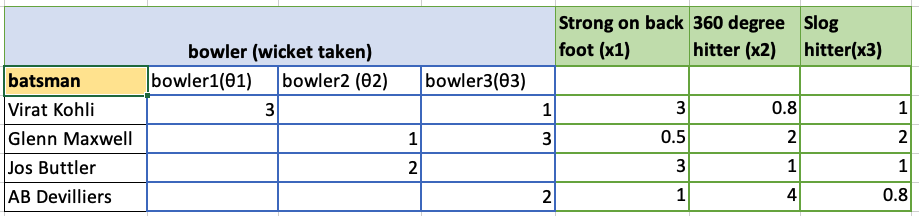
The Recommender Engine works as follows. Let us say that there are feature vectors $x^1$ , $x^2$ and $x^3$ for the 3 bowlers which identify the characteristics of these bowlers (“fast”, “lateral drift through the air”, “movement off the pitch”). Let each batsman be identified by parameter vectors $\theta^1$ , $\theta^2$ and so on

For e.g. consider the following table

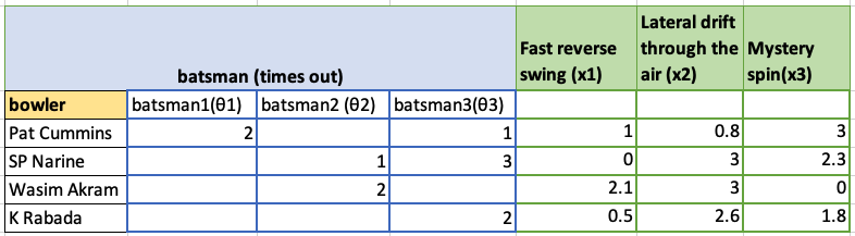
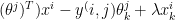
Then by assuming an initial estimate for the parameter vector $\theta$ and the feature vector xx we can formulate this as an optimization problem which tries to minimize the error for $\theta^T*x$ This can work very well as the algorithm can determine features which cannot be captured. So for e.g. some particular bowler may have very impressive figures. This could be due to some aspect of the bowling which cannot be captured by the data for e.g. let’s say the bowler uses the ‘scrambled seam’ when he is most effective, with a slightly different arc to the flight. Though the algorithm cannot identify the feature as we know it, but the ML algorithm should pick up intricacies which cannot be captured in data.

Hence the algorithm can be quite effective.

Note: The recommender lab performance is not very good and the Mean Square Error is quite high. Also, the ROC and AUC curves show that not in aLL cases the algorithm is doing a clean job of separating the True positives (TPR) from the False Positives (FPR)

Note: This is similar to the recommendation problem

The collaborative optimization object can be considered as a minimization of both $\theta$ and the features x and can be written as

J( $x^{(1)},x^{(2)},..x^{(n_{u})}$ , $\theta^{(1)},\theta^{(2)},..,\theta^{(n_{m})}$ }= 1/2 $\sum(\theta^{j})^{T}x^{i}- y^{(i,j)})^{2} + \lambda\sum\sum (x_{k}^{i})^{2} + \lambda\sum\sum (_\theta{k}^{j})^{2}$

The collaborative filtering algorithm can be summarized as follows

Initialize $\theta^1$ , $\theta^2$ … $\theta^{n_{u}}$ and the set of features be $x^1$ , $x^2$ , … , $x^{n_{m}}$ to small random values
Minimize J( $\theta^1$ , $\theta^2$ … $\theta^{n_{u}}$ , $x^1$ , $x^2$ , … , $x^{n_{m}}$ ) using gradient descent. For every
j=1,2, … $n_{u}$ , i= 1,2,.., $n_{m}$
$x_{k}^{i}$ := $x_{k}^{i}$ – $\alpha$ ( $\sigma$ $(\theta^j)^T$ ) $x^i$ – $y^(i,j)\theta_{k}^{j} + \lambda x_{k}^i$

&

$\theta_{k}^{i}$ := $\theta_{k}^{i}$ – $\alpha$ ( $\sigma$ $(\theta^j)^T)x^i - y^(i,j)\theta_{k}^{j} + \lambda x_{k}^i$
Hence for a batsman with parameters $\theta$ and a bowler with (learned) features x, predict the “times out” for the player where the value is not known using $\theta^Tx$

The above derivation for the recommender problem is taken from Machine Learning by Prof Andrew Ng at Coursera from the lecture Collaborative filtering

There are 2 main types of Collaborative Filtering(CF) approaches

User based Collaborative Filtering User-based CF is a memory-based algorithm which tries to mimics word-of-mouth by analyzing rating data from many individuals. The assumption is that users with similar preferences will rate items similarly.
Item based Collaborative Filtering Item-based CF is a model-based approach which produces recommendations based on the relationship between items inferred from the rating matrix. The assumption behind this approach is that users will prefer items that are similar to other items they like.

1a. A note on ROC and Precision-Recall curves

A small note on interpreting ROC & Precision-Recall curves in the post below

ROC Curve: The ROC curve plots the True Positive Rate (TPR) against the False Positive Rate (FPR). Ideally the TPR should increase faster than the FPR and the AUC (area under the curve) should be close to 1

Precision-Recall: The precision-recall curve shows the tradeoff between precision and recall for different threshold. A high area under the curve represents both high recall and high precision, where high precision relates to a low false positive rate, and high recall relates to a low false negative rate

library(reshape2)
library(dplyr)
library(ggplot2)
library(recommenderlab)
library(tidyr)
load("recom_data/batsmenVsBowler20_22.rdata")

2. Define recommender lab helper functions

Helper functions for the RMarkdown notebook are created

eval – Gives details of RMSE, MSE and MAE of ML algorithm
evalRecomMethods – Evaluates different recommender methods and plot the ROC and Precision-Recall curves

# This function returns the error for the chosen algorithm and also predicts the estimates
# for the given data
eval <- function(data, train1, k1,given1,goodRating1,recomType1="UBCF"){
  set.seed(2022)
  e<- evaluationScheme(data,
                       method = "split",
                       train = train1,
                       k = k1,
                       given = given1,
                       goodRating = goodRating1)
  
  r1 <- Recommender(getData(e, "train"), recomType1)
  print(r1)
  
  p1 <- predict(r1, getData(e, "known"), type="ratings")
  print(p1)
  
  error = calcPredictionAccuracy(p1, getData(e, "unknown"))
  
  print(error)
  p2 <- predict(r1, data, type="ratingMatrix")
  p2
}
# This function will evaluate the different recommender algorithms and plot the AUC and ROC curves
evalRecomMethods <- function(data,k1,given1,goodRating1){
  set.seed(2022)
  e<- evaluationScheme(data,
                       method = "cross",
                       k = k1,
                       given = given1,
                       goodRating = goodRating1)
  
  models_to_evaluate <- list(
    `IBCF Cosinus` = list(name = "IBCF", 
                          param = list(method = "cosine")),
    `IBCF Pearson` = list(name = "IBCF", 
                          param = list(method = "pearson")),
    `UBCF Cosinus` = list(name = "UBCF",
                          param = list(method = "cosine")),
    `UBCF Pearson` = list(name = "UBCF",
                          param = list(method = "pearson")),
    `Zufälliger Vorschlag` = list(name = "RANDOM", param=NULL)
  )
  
  n_recommendations <- c(1, 5, seq(10, 100, 10))
  list_results <- evaluate(x = e, 
                           method = models_to_evaluate, 
                           n = n_recommendations)
  plot(list_results, annotate=c(1,3), legend="bottomright")
  plot(list_results, "prec/rec", annotate=3, legend="topleft")
}

3. Batsman performance estimation

The section below regenerates the performance for batsmen based on incomplete data for the different fields in the data frame namely balls faced, fours, sixes, strike rate, times out. The recommender lab allows one to test several different algorithms all at once namely

User based – Cosine similarity method, Pearson similarity
Item based – Cosine similarity method, Pearson similarity
Popular
Random
SVD and a few others

3a. Batting dataframe

head(df)

##   batsman1         bowler1 ballsFaced totalRuns fours sixes  SR timesOut
## 1 A Badoni        A Mishra          0         0     0     0 NaN        0
## 2 A Badoni        A Nortje          0         0     0     0 NaN        0
## 3 A Badoni         A Zampa          0         0     0     0 NaN        0
## 4 A Badoni     Abdul Samad          0         0     0     0 NaN        0
## 5 A Badoni Abhishek Sharma          0         0     0     0 NaN        0
## 6 A Badoni      AD Russell          0         0     0     0 NaN        0

3b Data set and data preparation

For this analysis the data from Cricsheet has been processed using my R package yorkr to obtain the following 2 data sets – batsmenVsBowler – This dataset will contain the performance of the batsmen against the bowler and will capture a) ballsFaced b) totalRuns c) Fours d) Sixes e) SR f) timesOut – bowlerVsBatsmen – This data set will contain the performance of the bowler against the difference batsmen and will include a) deliveries b) runsConceded c) EconomyRate d) wicketsTaken

Obviously many rows/columns will be empty

This is a large data set and hence I have filtered for the period > Jan 2020 and < Dec 2022 which gives 2 datasets a) batsmanVsBowler20_22.rdata b) bowlerVsBatsman20_22.rdata

I also have 2 other datasets of all batsmen and bowlers in these 2 dataset in the files c) all-batsmen20_22.rds d) all-bowlers20_22.rds

You can download the data and this RMarkdown notebook from Github at PlayerPerformanceEstimation

Feel free to download and analyze the data and use any recommendation engine you choose

3c. Exploratory analysis

Initially an exploratory analysis is done on the data

df3 <- select(df, batsman1,bowler1,timesOut)
df6 <- xtabs(timesOut ~ ., df3)
df7 <- as.data.frame.matrix(df6)
df8 <- data.matrix(df7)
df8[df8 == 0] <- NA
print(df8[1:10,1:10])

##                 A Mishra A Nortje A Zampa Abdul Samad Abhishek Sharma
## A Badoni              NA       NA      NA          NA              NA
## A Manohar             NA       NA      NA          NA              NA
## A Nortje              NA       NA      NA          NA              NA
## AB de Villiers        NA        4       3          NA              NA
## Abdul Samad           NA       NA      NA          NA              NA
## Abhishek Sharma       NA       NA      NA          NA              NA
## AD Russell             1       NA      NA          NA              NA
## AF Milne              NA       NA      NA          NA              NA
## AJ Finch              NA       NA      NA          NA               3
## AJ Tye                NA       NA      NA          NA              NA
##                 AD Russell AF Milne AJ Tye AK Markram Akash Deep
## A Badoni                NA       NA     NA         NA         NA
## A Manohar               NA       NA     NA         NA         NA
## A Nortje                NA       NA     NA         NA         NA
## AB de Villiers           3       NA      3         NA         NA
## Abdul Samad             NA       NA     NA         NA         NA
## Abhishek Sharma         NA       NA     NA         NA         NA
## AD Russell              NA       NA      6         NA         NA
## AF Milne                NA       NA     NA         NA         NA
## AJ Finch                NA       NA     NA         NA         NA
## AJ Tye                  NA       NA     NA         NA         NA

The dots below represent data for which there is no performance data. These cells need to be estimated by the algorithm

set.seed(2022)
r <- as(df8,"realRatingMatrix")
getRatingMatrix(r)[1:15,1:15]

## 15 x 15 sparse Matrix of class "dgCMatrix"

##    [[ suppressing 15 column names 'A Mishra', 'A Nortje', 'A Zampa' ... ]]

##                                               
## A Badoni         . . . . . . . . . . . . . . .
## A Manohar        . . . . . . . . . . . . . . .
## A Nortje         . . . . . . . . . . . . . . .
## AB de Villiers   . 4 3 . . 3 . 3 . . . 4 3 . .
## Abdul Samad      . . . . . . . . . . . . . . .
## Abhishek Sharma  . . . . . . . . . . . 1 . . .
## AD Russell       1 . . . . . . 6 . . . 3 3 3 .
## AF Milne         . . . . . . . . . . . . . . .
## AJ Finch         . . . . 3 . . . . . . 1 . . .
## AJ Tye           . . . . . . . . . . . 1 . . .
## AK Markram       . . . 3 . . . . . . . . . . .
## AM Rahane        9 . . . . 3 . 3 . . . 3 3 . .
## Anmolpreet Singh . . . . . . . . . . . . . . .
## Anuj Rawat       . . . . . . . . . . . . . . .
## AR Patel         . . . . . . . 1 . . . . . . .

r0=r[(rowCounts(r) > 10),]
getRatingMatrix(r0)[1:15,1:15]

## 15 x 15 sparse Matrix of class "dgCMatrix"

##    [[ suppressing 15 column names 'A Mishra', 'A Nortje', 'A Zampa' ... ]]

##                                              
## AB de Villiers  . 4 3 . . 3 . 3 . . . 4 3 . .
## Abdul Samad     . . . . . . . . . . . . . . .
## Abhishek Sharma . . . . . . . . . . . 1 . . .
## AD Russell      1 . . . . . . 6 . . . 3 3 3 .
## AJ Finch        . . . . 3 . . . . . . 1 . . .
## AM Rahane       9 . . . . 3 . 3 . . . 3 3 . .
## AR Patel        . . . . . . . 1 . . . . . . .
## AT Rayudu       2 . . . . . 1 . . . . 3 . . .
## B Kumar         3 . 3 . . . . . . . . . . 3 .
## BA Stokes       . . . . . . 3 4 . . . 3 . . .
## CA Lynn         . . . . . . . 9 . . . 3 . . .
## CH Gayle        . . . . . 6 . 3 . . . 6 . . .
## CH Morris       . 3 . . . . . . . . . 3 . . .
## D Padikkal      . 4 . . . 3 . . . . . . 3 . .
## DA Miller       . . . . . 3 . . . . . 3 . . .

# Get the summary of the data
summary(getRatings(r0))

##    Min. 1st Qu.  Median    Mean 3rd Qu.    Max. 
##   1.000   3.000   3.000   3.463   4.000  21.000

# Normalize the data
r0_m <- normalize(r0)
getRatingMatrix(r0_m)[1:15,1:15]

## 15 x 15 sparse Matrix of class "dgCMatrix"

##    [[ suppressing 15 column names 'A Mishra', 'A Nortje', 'A Zampa' ... ]]

##                                                                       
## AB de Villiers   .         -0.7857143 -1.7857143 .  .       -1.7857143
## Abdul Samad      .          .          .         .  .        .        
## Abhishek Sharma  .          .          .         .  .        .        
## AD Russell      -2.6562500  .          .         .  .        .        
## AJ Finch         .          .          .         . -0.03125  .        
## AM Rahane        4.6041667  .          .         .  .       -1.3958333
## AR Patel         .          .          .         .  .        .        
## AT Rayudu       -2.1363636  .          .         .  .        .        
## B Kumar          0.3636364  .          0.3636364 .  .        .        
## BA Stokes        .          .          .         .  .        .        
## CA Lynn          .          .          .         .  .        .        
## CH Gayle         .          .          .         .  .        1.5476190
## CH Morris        .          0.3500000  .         .  .        .        
## D Padikkal       .          0.6250000  .         .  .       -0.3750000
## DA Miller        .          .          .         .  .       -0.7037037
##                                                                              
## AB de Villiers   .         -1.7857143 . . . -0.7857143 -1.785714  .         .
## Abdul Samad      .          .         . . .  .          .         .         .
## Abhishek Sharma  .          .         . . . -1.6000000  .         .         .
## AD Russell       .          2.3437500 . . . -0.6562500 -0.656250 -0.6562500 .
## AJ Finch         .          .         . . . -2.0312500  .         .         .
## AM Rahane        .         -1.3958333 . . . -1.3958333 -1.395833  .         .
## AR Patel         .         -2.3333333 . . .  .          .         .         .
## AT Rayudu       -3.1363636  .         . . . -1.1363636  .         .         .
## B Kumar          .          .         . . .  .          .         0.3636364 .
## BA Stokes       -0.6086957  0.3913043 . . . -0.6086957  .         .         .
## CA Lynn          .          5.3200000 . . . -0.6800000  .         .         .
## CH Gayle         .         -1.4523810 . . .  1.5476190  .         .         .
## CH Morris        .          .         . . .  0.3500000  .         .         .
## D Padikkal       .          .         . . .  .         -0.375000  .         .
## DA Miller        .          .         . . . -0.7037037  .         .         .

4. Create a visual representation of the rating data before and after the normalization

The histograms show the bias in the data is removed after normalization

r0=r[(m=rowCounts(r) > 10),]
getRatingMatrix(r0)[1:15,1:10]

## 15 x 10 sparse Matrix of class "dgCMatrix"

##    [[ suppressing 10 column names 'A Mishra', 'A Nortje', 'A Zampa' ... ]]

##                                    
## AB de Villiers  . 4 3 . . 3 . 3 . .
## Abdul Samad     . . . . . . . . . .
## Abhishek Sharma . . . . . . . . . .
## AD Russell      1 . . . . . . 6 . .
## AJ Finch        . . . . 3 . . . . .
## AM Rahane       9 . . . . 3 . 3 . .
## AR Patel        . . . . . . . 1 . .
## AT Rayudu       2 . . . . . 1 . . .
## B Kumar         3 . 3 . . . . . . .
## BA Stokes       . . . . . . 3 4 . .
## CA Lynn         . . . . . . . 9 . .
## CH Gayle        . . . . . 6 . 3 . .
## CH Morris       . 3 . . . . . . . .
## D Padikkal      . 4 . . . 3 . . . .
## DA Miller       . . . . . 3 . . . .

#Plot ratings
image(r0, main = "Raw Ratings")

#Plot normalized ratings
r0_m <- normalize(r0)
getRatingMatrix(r0_m)[1:15,1:15]

## 15 x 15 sparse Matrix of class "dgCMatrix"

##    [[ suppressing 15 column names 'A Mishra', 'A Nortje', 'A Zampa' ... ]]

##                                                                       
## AB de Villiers   .         -0.7857143 -1.7857143 .  .       -1.7857143
## Abdul Samad      .          .          .         .  .        .        
## Abhishek Sharma  .          .          .         .  .        .        
## AD Russell      -2.6562500  .          .         .  .        .        
## AJ Finch         .          .          .         . -0.03125  .        
## AM Rahane        4.6041667  .          .         .  .       -1.3958333
## AR Patel         .          .          .         .  .        .        
## AT Rayudu       -2.1363636  .          .         .  .        .        
## B Kumar          0.3636364  .          0.3636364 .  .        .        
## BA Stokes        .          .          .         .  .        .        
## CA Lynn          .          .          .         .  .        .        
## CH Gayle         .          .          .         .  .        1.5476190
## CH Morris        .          0.3500000  .         .  .        .        
## D Padikkal       .          0.6250000  .         .  .       -0.3750000
## DA Miller        .          .          .         .  .       -0.7037037
##                                                                              
## AB de Villiers   .         -1.7857143 . . . -0.7857143 -1.785714  .         .
## Abdul Samad      .          .         . . .  .          .         .         .
## Abhishek Sharma  .          .         . . . -1.6000000  .         .         .
## AD Russell       .          2.3437500 . . . -0.6562500 -0.656250 -0.6562500 .
## AJ Finch         .          .         . . . -2.0312500  .         .         .
## AM Rahane        .         -1.3958333 . . . -1.3958333 -1.395833  .         .
## AR Patel         .         -2.3333333 . . .  .          .         .         .
## AT Rayudu       -3.1363636  .         . . . -1.1363636  .         .         .
## B Kumar          .          .         . . .  .          .         0.3636364 .
## BA Stokes       -0.6086957  0.3913043 . . . -0.6086957  .         .         .
## CA Lynn          .          5.3200000 . . . -0.6800000  .         .         .
## CH Gayle         .         -1.4523810 . . .  1.5476190  .         .         .
## CH Morris        .          .         . . .  0.3500000  .         .         .
## D Padikkal       .          .         . . .  .         -0.375000  .         .
## DA Miller        .          .         . . . -0.7037037  .         .         .

image(r0_m, main = "Normalized Ratings")

set.seed(1234)
hist(getRatings(r0), breaks=25)

hist(getRatings(r0_m), breaks=25)

4a. Data for analysis

The data frame of the batsman vs bowlers from the period 2020 -2022 is read as a dataframe. To remove rows with very low number of ratings(timesOut, SR, Fours, Sixes etc), the rows are filtered so that there are at least more 10 values in the row. For the player estimation the dataframe is converted into a wide-format as a matrix (m x n) of batsman x bowler with each of the columns of the dataframe i.e. timesOut, SR, fours or sixes. These different matrices can be considered as a rating matrix for estimation.

A similar approach is taken for estimating bowler performance. Here a wide form matrix (m x n) of bowler x batsman is created for each of the columns of deliveries, runsConceded, ER, wicketsTaken

5. Batsman’s times Out

The code below estimates the number of times the batsmen would lose his/her wicket to the bowler. As discussed in the algorithm above, the recommendation engine will make an initial estimate features for the bowler and an initial estimate for the parameter vector for the batsmen. Then using gradient descent the recommender engine will determine the feature and parameter values such that the over Mean Squared Error is minimum

From the plot for the different algorithms it can be seen that UBCF performs the best. However the AUC & ROC curves are not optimal and the AUC> 0.5

df3 <- select(df, batsman1,bowler1,timesOut)
df6 <- xtabs(timesOut ~ ., df3)
df7 <- as.data.frame.matrix(df6)
df8 <- data.matrix(df7)
df8[df8 == 0] <- NA
r <- as(df8,"realRatingMatrix")
# Filter only rows where the row count is > 10
r0=r[(rowCounts(r) > 10),]
getRatingMatrix(r0)[1:10,1:10]

## 10 x 10 sparse Matrix of class "dgCMatrix"

##    [[ suppressing 10 column names 'A Mishra', 'A Nortje', 'A Zampa' ... ]]

##                                    
## AB de Villiers  . 4 3 . . 3 . 3 . .
## Abdul Samad     . . . . . . . . . .
## Abhishek Sharma . . . . . . . . . .
## AD Russell      1 . . . . . . 6 . .
## AJ Finch        . . . . 3 . . . . .
## AM Rahane       9 . . . . 3 . 3 . .
## AR Patel        . . . . . . . 1 . .
## AT Rayudu       2 . . . . . 1 . . .
## B Kumar         3 . 3 . . . . . . .
## BA Stokes       . . . . . . 3 4 . .

summary(getRatings(r0))

##    Min. 1st Qu.  Median    Mean 3rd Qu.    Max. 
##   1.000   3.000   3.000   3.463   4.000  21.000

# Evaluate the different plotting methods
evalRecomMethods(r0[1:dim(r0)[1]],k1=5,given=7,goodRating1=median(getRatings(r0)))

#Evaluate the error
a=eval(r0[1:dim(r0)[1]],0.8,k1=5,given1=7,goodRating1=median(getRatings(r0)),"UBCF")

## Recommender of type 'UBCF' for 'realRatingMatrix' 
## learned using 70 users.
## 18 x 145 rating matrix of class 'realRatingMatrix' with 1755 ratings.
##     RMSE      MSE      MAE 
## 2.069027 4.280872 1.496388

b=round(as(a,"matrix")[1:10,1:10])
c <- as(b,"realRatingMatrix")
m=as(c,"data.frame")
names(m) =c("batsman","bowler","TimesOut")

6. Batsman’s Strike rate

This section deals with the Strike rate of batsmen versus bowlers and estimates the values for those where the data is incomplete using UBCF method.

Even here all the algorithms do not perform too efficiently. I did try out a few variations but could not lower the error (suggestions welcome!!)

df3 <- select(df, batsman1,bowler1,SR)
df6 <- xtabs(SR ~ ., df3)
df7 <- as.data.frame.matrix(df6)
df8 <- data.matrix(df7)
df8[df8 == 0] <- NA
r <- as(df8,"realRatingMatrix")
r0=r[(rowCounts(r) > 10),]
getRatingMatrix(r0)[1:10,1:10]

## 10 x 10 sparse Matrix of class "dgCMatrix"

##    [[ suppressing 10 column names 'A Mishra', 'A Nortje', 'A Zampa' ... ]]

##                                                                           
## AB de Villiers   96.8254 171.4286  33.33333  . 66.66667 223.07692   .     
## Abdul Samad       .      228.0000   .        .  .       100.00000   .     
## Abhishek Sharma 150.0000   .        .        .  .        66.66667   .     
## AD Russell      111.4286   .        .        .  .         .         .     
## AJ Finch        250.0000 116.6667   .        . 50.00000  85.71429 112.5000
## AJ Tye            .        .        .        .  .         .       100.0000
## AK Markram        .        .        .       50  .         .         .     
## AM Rahane       121.1111   .        .        .  .       113.82979 117.9487
## AR Patel        183.3333   .      200.00000  .  .       433.33333   .     
## AT Rayudu       126.5432 200.0000 122.22222  .  .       105.55556   .     
##                                
## AB de Villiers  109.52381 .   .
## Abdul Samad       .       .   .
## Abhishek Sharma   .       .   .
## AD Russell      195.45455 .   .
## AJ Finch          .       .   .
## AJ Tye            .       .   .
## AK Markram        .       .   .
## AM Rahane        33.33333 . 200
## AR Patel        171.42857 .   .
## AT Rayudu       204.76190 .   .

summary(getRatings(r0))

##    Min. 1st Qu.  Median    Mean 3rd Qu.    Max. 
##   5.882  85.714 116.667 128.529 160.606 600.000

evalRecomMethods(r0[1:dim(r0)[1]],k1=5,given=7,goodRating1=median(getRatings(r0)))

a=eval(r0[1:dim(r0)[1]],0.8, k1=5,given1=7,goodRating1=median(getRatings(r0)),"UBCF")

## Recommender of type 'UBCF' for 'realRatingMatrix' 
## learned using 105 users.
## 27 x 145 rating matrix of class 'realRatingMatrix' with 3220 ratings.
##       RMSE        MSE        MAE 
##   77.71979 6040.36508   58.58484

b=round(as(a,"matrix")[1:10,1:10])
c <- as(b,"realRatingMatrix")
n=as(c,"data.frame")
names(n) =c("batsman","bowler","SR")

7. Batsman’s Sixes

The snippet of code estimes the sixes of the batsman against bowlers. The ROC and AUC curve for UBCF looks a lot better here, as it significantly greater than 0.5

df3 <- select(df, batsman1,bowler1,sixes)
df6 <- xtabs(sixes ~ ., df3)
df7 <- as.data.frame.matrix(df6)
df8 <- data.matrix(df7)
df8[df8 == 0] <- NA
r <- as(df8,"realRatingMatrix")
r0=r[(rowCounts(r) > 10),]
getRatingMatrix(r0)[1:10,1:10]

## 10 x 10 sparse Matrix of class "dgCMatrix"

##    [[ suppressing 10 column names 'A Mishra', 'A Nortje', 'A Zampa' ... ]]

##                                      
## AB de Villiers  3 3 . . . 18 .  3 . .
## AD Russell      3 . . . .  . . 12 . .
## AJ Finch        2 . . . .  . .  . . .
## AM Rahane       7 . . . .  3 1  . . .
## AR Patel        4 . 3 . .  6 .  1 . .
## AT Rayudu       5 2 . . .  . .  1 . .
## BA Stokes       . . . . .  . .  . . .
## CA Lynn         . . . . .  . .  9 . .
## CH Gayle       17 . . . . 17 .  . . .
## CH Morris       . . 3 . .  . .  . . .

summary(getRatings(r0))

##    Min. 1st Qu.  Median    Mean 3rd Qu.    Max. 
##    1.00    3.00    3.00    4.68    6.00   33.00

evalRecomMethods(r0[1:dim(r0)[1]],k1=5,given=7,goodRating1=median(getRatings(r0)))

## Timing stopped at: 0.003 0 0.002

a=eval(r0[1:dim(r0)[1]],0.8, k1=5,given1=7,goodRating1=median(getRatings(r0)),"UBCF")

## Recommender of type 'UBCF' for 'realRatingMatrix' 
## learned using 52 users.
## 14 x 145 rating matrix of class 'realRatingMatrix' with 1634 ratings.
##      RMSE       MSE       MAE 
##  3.529922 12.460350  2.532122

b=round(as(a,"matrix")[1:10,1:10])
c <- as(b,"realRatingMatrix")
o=as(c,"data.frame")
names(o) =c("batsman","bowler","Sixes")

8. Batsman’s Fours

The code below estimates 4s for the batsmen

df3 <- select(df, batsman1,bowler1,fours)
df6 <- xtabs(fours ~ ., df3)
df7 <- as.data.frame.matrix(df6)
df8 <- data.matrix(df7)
df8[df8 == 0] <- NA
r <- as(df8,"realRatingMatrix")
r0=r[(rowCounts(r) > 10),]
getRatingMatrix(r0)[1:10,1:10]

## 10 x 10 sparse Matrix of class "dgCMatrix"

##    [[ suppressing 10 column names 'A Mishra', 'A Nortje', 'A Zampa' ... ]]

##                                      
## AB de Villiers   . 1 . . . 24 . 3 . .
## Abhishek Sharma  . . . . .  . . . . .
## AD Russell       1 . . . .  . . 9 . .
## AJ Finch         . 1 . . .  3 2 . . .
## AK Markram       . . . . .  . . . . .
## AM Rahane       11 . . . .  8 7 . . 3
## AR Patel         . . . . .  . . 3 . .
## AT Rayudu       11 2 3 . .  6 . 6 . .
## BA Stokes        1 . . . .  . . . . .
## CA Lynn          . . . . .  . . 6 . .

summary(getRatings(r0))

##    Min. 1st Qu.  Median    Mean 3rd Qu.    Max. 
##   1.000   3.000   4.000   6.339   9.000  55.000

evalRecomMethods(r0[1:dim(r0)[1]],k1=5,given=7,goodRating1=median(getRatings(r0)))

## Timing stopped at: 0.008 0 0.008

## Warning in .local(x, method, ...): 
##   Recommender 'UBCF Pearson' has failed and has been removed from the results!

a=eval(r0[1:dim(r0)[1]],0.8, k1=5,given1=7,goodRating1=median(getRatings(r0)),"UBCF")

## Recommender of type 'UBCF' for 'realRatingMatrix' 
## learned using 67 users.
## 17 x 145 rating matrix of class 'realRatingMatrix' with 2083 ratings.
##      RMSE       MSE       MAE 
##  5.486661 30.103447  4.060990

b=round(as(a,"matrix")[1:10,1:10])
c <- as(b,"realRatingMatrix")
p=as(c,"data.frame")
names(p) =c("batsman","bowler","Fours")

9. Batsman’s Total Runs

The code below estimates the total runs that would have scored by the batsman against different bowlers

df3 <- select(df, batsman1,bowler1,totalRuns)
df6 <- xtabs(totalRuns ~ ., df3)
df7 <- as.data.frame.matrix(df6)
df8 <- data.matrix(df7)
df8[df8 == 0] <- NA
r <- as(df8,"realRatingMatrix")
r0=r[(rowCounts(r) > 10),]
getRatingMatrix(r)[1:10,1:10]

## 10 x 10 sparse Matrix of class "dgCMatrix"

##    [[ suppressing 10 column names 'A Mishra', 'A Nortje', 'A Zampa' ... ]]

##                                          
## A Badoni         .  . . . .   . .   . . .
## A Manohar        .  . . . .   . .   . . .
## A Nortje         .  . . . .   . .   . . .
## AB de Villiers  61 36 3 . 6 261 .  69 . .
## Abdul Samad      . 57 . . .  12 .   . . .
## Abhishek Sharma  3  . . . .   6 .   . . .
## AD Russell      39  . . . .   . . 129 . .
## AF Milne         .  . . . .   . .   . . .
## AJ Finch        15  7 . . 3  18 9   . . .
## AJ Tye           .  . . . .   . 4   . . .

summary(getRatings(r0))

##    Min. 1st Qu.  Median    Mean 3rd Qu.    Max. 
##    1.00    9.00   24.00   41.36   54.00  452.00

evalRecomMethods(r0[1:dim(r0)[1]],k1=5,given1=7,goodRating1=median(getRatings(r0)))

a=eval(r0[1:dim(r0)[1]],0.8, k1=5,given1=7,goodRating1=median(getRatings(r0)),"UBCF")

## Recommender of type 'UBCF' for 'realRatingMatrix' 
## learned using 105 users.
## 27 x 145 rating matrix of class 'realRatingMatrix' with 3256 ratings.
##       RMSE        MSE        MAE 
##   41.50985 1723.06788   29.52958

b=round(as(a,"matrix")[1:10,1:10])
c <- as(b,"realRatingMatrix")
q=as(c,"data.frame")
names(q) =c("batsman","bowler","TotalRuns")

10. Batsman’s Balls Faced

The snippet estimates the balls faced by batsmen versus bowlers

df3 <- select(df, batsman1,bowler1,ballsFaced)
df6 <- xtabs(ballsFaced ~ ., df3)
df7 <- as.data.frame.matrix(df6)
df8 <- data.matrix(df7)
df8[df8 == 0] <- NA
r <- as(df8,"realRatingMatrix")
r0=r[(rowCounts(r) > 10),]
getRatingMatrix(r)[1:10,1:10]

## 10 x 10 sparse Matrix of class "dgCMatrix"

##    [[ suppressing 10 column names 'A Mishra', 'A Nortje', 'A Zampa' ... ]]

##                                         
## A Badoni         .  . . . .   . .  . . .
## A Manohar        .  . . . .   . .  . . .
## A Nortje         .  . . . .   . .  . . .
## AB de Villiers  63 21 9 . 9 117 . 63 . .
## Abdul Samad      . 25 . . .  12 .  . . .
## Abhishek Sharma  2  . . . .   9 .  . . .
## AD Russell      35  . . . .   . . 66 . .
## AF Milne         .  . . . .   . .  . . .
## AJ Finch         6  6 . . 6  21 8  . . .
## AJ Tye           .  . . . .   9 4  . . .

summary(getRatings(r0))

##    Min. 1st Qu.  Median    Mean 3rd Qu.    Max. 
##    1.00    9.00   18.00   30.21   39.00  384.00

evalRecomMethods(r0[1:dim(r0)[1]],k1=5,given=7,goodRating1=median(getRatings(r0)))

a=eval(r0[1:dim(r0)[1]],0.8, k1=5,given1=7,goodRating1=median(getRatings(r0)),"UBCF")

## Recommender of type 'UBCF' for 'realRatingMatrix' 
## learned using 112 users.
## 28 x 145 rating matrix of class 'realRatingMatrix' with 3378 ratings.
##       RMSE        MSE        MAE 
##   33.91251 1150.05835   23.39439

b=round(as(a,"matrix")[1:10,1:10])
c <- as(b,"realRatingMatrix")
r=as(c,"data.frame")
names(r) =c("batsman","bowler","BallsFaced")

11. Generate the Batsmen Performance Estimate

This code generates the estimated dataframe with known and ‘predicted’ values

a1=merge(m,n,by=c("batsman","bowler"))
a2=merge(a1,o,by=c("batsman","bowler"))
a3=merge(a2,p,by=c("batsman","bowler"))
a4=merge(a3,q,by=c("batsman","bowler"))
a5=merge(a4,r,by=c("batsman","bowler"))
a6= select(a5, batsman,bowler,BallsFaced,TotalRuns,Fours, Sixes, SR,TimesOut)
head(a6)

##          batsman          bowler BallsFaced TotalRuns Fours Sixes  SR TimesOut
## 1 AB de Villiers        A Mishra         94       124     7     5 144        5
## 2 AB de Villiers        A Nortje         26        42     4     3 148        3
## 3 AB de Villiers         A Zampa         28        42     5     7 106        4
## 4 AB de Villiers Abhishek Sharma         22        28     0    10 136        5
## 5 AB de Villiers      AD Russell         70       135    14    12 207        4
## 6 AB de Villiers        AF Milne         31        45     6     6 130        3

12. Bowler analysis

Just like the batsman performance estimation we can consider the bowler’s performances also for estimation. Consider the following table

As in the batsman analysis, for every batsman a set of features like (“strong backfoot player”, “360 degree player”,“Power hitter”) can be estimated with a set of initial values. Also every bowler will have an associated parameter vector θθ. Different bowlers will have performance data for different set of batsmen. Based on the initial estimate of the features and the parameters, gradient descent can be used to minimize actual values {for e.g. wicketsTaken(ratings)}.

load("recom_data/bowlerVsBatsman20_22.rdata")

12a. Bowler dataframe

Inspecting the bowler dataframe

head(df2)

##    bowler1        batsman1 balls runsConceded       ER wicketTaken
## 1 A Mishra        A Badoni     0            0 0.000000           0
## 2 A Mishra       A Manohar     0            0 0.000000           0
## 3 A Mishra        A Nortje     0            0 0.000000           0
## 4 A Mishra  AB de Villiers    63           61 5.809524           0
## 5 A Mishra     Abdul Samad     0            0 0.000000           0
## 6 A Mishra Abhishek Sharma     2            3 9.000000           0

names(df2)

## [1] "bowler1"      "batsman1"     "balls"        "runsConceded" "ER"          
## [6] "wicketTaken"

13. Balls bowled by bowler

The below section estimates the balls bowled for each bowler. We can see that UBCF Pearson and UBCF Cosine both perform well

df3 <- select(df2, bowler1,batsman1,balls)
df6 <- xtabs(balls ~ ., df3)
df7 <- as.data.frame.matrix(df6)
df8 <- data.matrix(df7)
df8[df8 == 0] <- NA
r <- as(df8,"realRatingMatrix")
r0=r[(rowCounts(r) > 10),]
getRatingMatrix(r0)[1:10,1:10]

## 10 x 10 sparse Matrix of class "dgCMatrix"

##    [[ suppressing 10 column names 'A Badoni', 'A Manohar', 'A Nortje' ... ]]

##                                          
## A Mishra        . . .  63  .  2 35 .  6 .
## A Nortje        . . .  21 25  .  . .  6 .
## A Zampa         . . .   9  .  .  . .  . .
## Abhishek Sharma . . .   9  .  .  . .  6 .
## AD Russell      . . . 117 12  9  . . 21 9
## AF Milne        . . .   .  .  .  . .  8 4
## AJ Tye          . . .  63  .  . 66 .  . .
## Akash Deep      . . .   .  .  .  . .  . .
## AR Patel        . . . 188  5  1 84 . 29 5
## Arshdeep Singh  . . .   6  6 24 18 . 12 .

summary(getRatings(r0))

##    Min. 1st Qu.  Median    Mean 3rd Qu.    Max. 
##    1.00    9.00   18.00   29.61   36.00  384.00

evalRecomMethods(r0[1:dim(r0)[1]],k1=5,given=7,goodRating1=median(getRatings(r0)))

a=eval(r0[1:dim(r0)[1]],0.8,k1=5,given1=7,goodRating1=median(getRatings(r0)),"UBCF")

## Recommender of type 'UBCF' for 'realRatingMatrix' 
## learned using 96 users.
## 24 x 195 rating matrix of class 'realRatingMatrix' with 3954 ratings.
##      RMSE       MSE       MAE 
##  30.72284 943.89294  19.89204

b=round(as(a,"matrix")[1:10,1:10])
c <- as(b,"realRatingMatrix")
s=as(c,"data.frame")
names(s) =c("bowler","batsman","BallsBowled")

14. Runs conceded by bowler

This section estimates the runs conceded by the bowler. The UBCF Cosinus algorithm performs the best with TPR increasing fastewr than FPR

df3 <- select(df2, bowler1,batsman1,runsConceded)
df6 <- xtabs(runsConceded ~ ., df3)
df7 <- as.data.frame.matrix(df6)
df8 <- data.matrix(df7)
df8[df8 == 0] <- NA
r <- as(df8,"realRatingMatrix")
r0=r[(rowCounts(r) > 10),]
getRatingMatrix(r0)[1:10,1:10]

## 10 x 10 sparse Matrix of class "dgCMatrix"

##    [[ suppressing 10 column names 'A Badoni', 'A Manohar', 'A Nortje' ... ]]

##                                            
## A Mishra        . . .  61  .  3  41 . 15  .
## A Nortje        . . .  36 57  .   . .  8  .
## A Zampa         . . .   3  .  .   . .  .  .
## Abhishek Sharma . . .   6  .  .   . .  3  .
## AD Russell      . . . 276 12  6   . . 21  .
## AF Milne        . . .   .  .  .   . . 10  4
## AJ Tye          . . .  69  .  . 138 .  .  .
## Akash Deep      . . .   .  .  .   . .  .  .
## AR Patel        . . . 205  5  . 165 . 33 13
## Arshdeep Singh  . . .  18  3 51  51 .  6  .

summary(getRatings(r0))

##    Min. 1st Qu.  Median    Mean 3rd Qu.    Max. 
##    1.00    9.00   24.00   41.34   54.00  458.00

evalRecomMethods(r0[1:dim(r0)[1]],k1=5,given=7,goodRating1=median(getRatings(r0)))

## Timing stopped at: 0.004 0 0.004

## Warning in .local(x, method, ...): 
##   Recommender 'UBCF Pearson' has failed and has been removed from the results!

a=eval(r0[1:dim(r0)[1]],0.8,k1=5,given1=7,goodRating1=median(getRatings(r0)),"UBCF")

## Recommender of type 'UBCF' for 'realRatingMatrix' 
## learned using 95 users.
## 24 x 195 rating matrix of class 'realRatingMatrix' with 3820 ratings.
##       RMSE        MSE        MAE 
##   43.16674 1863.36749   30.32709

b=round(as(a,"matrix")[1:10,1:10])
c <- as(b,"realRatingMatrix")
t=as(c,"data.frame")
names(t) =c("bowler","batsman","RunsConceded")

15. Economy Rate of the bowler

This section computes the economy rate of the bowler. The performance is not all that good

df3 <- select(df2, bowler1,batsman1,ER)
df6 <- xtabs(ER ~ ., df3)
df7 <- as.data.frame.matrix(df6)
df8 <- data.matrix(df7)
df8[df8 == 0] <- NA
r <- as(df8,"realRatingMatrix")
r0=r[(rowCounts(r) > 10),]
getRatingMatrix(r0)[1:10,1:10]

## 10 x 10 sparse Matrix of class "dgCMatrix"

##    [[ suppressing 10 column names 'A Badoni', 'A Manohar', 'A Nortje' ... ]]

##                                                                       
## A Mishra        . . .  5.809524  .     9.00  7.028571 . 15.000000  .  
## A Nortje        . . . 10.285714 13.68  .     .        .  8.000000  .  
## A Zampa         . . .  2.000000  .     .     .        .  .         .  
## Abhishek Sharma . . .  4.000000  .     .     .        .  3.000000  .  
## AD Russell      . . . 14.153846  6.00  4.00  .        .  6.000000  .  
## AF Milne        . . .  .         .     .     .        .  7.500000  6.0
## AJ Tye          . . .  6.571429  .     .    12.545455 .  .         .  
## Akash Deep      . . .  .         .     .     .        .  .         .  
## AR Patel        . . .  6.542553  6.00  .    11.785714 .  6.827586 15.6
## Arshdeep Singh  . . . 18.000000  3.00 12.75 17.000000 .  3.000000  .

summary(getRatings(r0))

##    Min. 1st Qu.  Median    Mean 3rd Qu.    Max. 
##  0.3529  5.2500  7.1126  7.8139  9.8000 36.0000

evalRecomMethods(r0[1:dim(r0)[1]],k1=5,given=7,goodRating1=median(getRatings(r0)))

## Timing stopped at: 0.003 0 0.004

## Warning in .local(x, method, ...): 
##   Recommender 'UBCF Pearson' has failed and has been removed from the results!

a=eval(r0[1:dim(r0)[1]],0.8,k1=5,given1=7,goodRating1=median(getRatings(r0)),"UBCF")

## Recommender of type 'UBCF' for 'realRatingMatrix' 
## learned using 95 users.
## 24 x 195 rating matrix of class 'realRatingMatrix' with 3839 ratings.
##      RMSE       MSE       MAE 
##  4.380680 19.190356  3.316556

b=round(as(a,"matrix")[1:10,1:10])
c <- as(b,"realRatingMatrix")
u=as(c,"data.frame")
names(u) =c("bowler","batsman","EconomyRate")

16. Wickets Taken by bowler

The code below computes the wickets taken by the bowler versus different batsmen

df3 <- select(df2, bowler1,batsman1,wicketTaken)
df6 <- xtabs(wicketTaken ~ ., df3)
df7 <- as.data.frame.matrix(df6)
df8 <- data.matrix(df7)
df8[df8 == 0] <- NA
r <- as(df8,"realRatingMatrix")
r0=r[(rowCounts(r) > 10),]
getRatingMatrix(r0)[1:10,1:10]

## 10 x 10 sparse Matrix of class "dgCMatrix"

##    [[ suppressing 10 column names 'A Badoni', 'A Manohar', 'A Nortje' ... ]]

##                                   
## A Mishra       . . . . . . 1 . . .
## A Nortje       . . . 4 . . . . . .
## A Zampa        . . . 3 . . . . . .
## AD Russell     . . . 3 . . . . . .
## AJ Tye         . . . 3 . . 6 . . .
## AR Patel       . . . 4 . 1 3 . 1 1
## Arshdeep Singh . . . 3 . . 3 . . .
## AS Rajpoot     . . . . . . 3 . . .
## Avesh Khan     . . . . . . 1 . 3 .
## B Kumar        . . . 9 . . 3 . 1 .

summary(getRatings(r0))

##    Min. 1st Qu.  Median    Mean 3rd Qu.    Max. 
##   1.000   3.000   3.000   3.423   3.000  21.000

evalRecomMethods(r0[1:dim(r0)[1]],k1=5,given=7,goodRating1=median(getRatings(r0)))

## Timing stopped at: 0.003 0 0.003

## Warning in .local(x, method, ...): 
##   Recommender 'UBCF Pearson' has failed and has been removed from the results!

a=eval(r0[1:dim(r0)[1]],0.8,k1=5,given1=7,goodRating1=median(getRatings(r0)),"UBCF")

## Recommender of type 'UBCF' for 'realRatingMatrix' 
## learned using 64 users.
## 16 x 195 rating matrix of class 'realRatingMatrix' with 1908 ratings.
##     RMSE      MSE      MAE 
## 2.672677 7.143203 1.956934

b=round(as(a,"matrix")[1:10,1:10])
c <- as(b,"realRatingMatrix")
v=as(c,"data.frame")
names(v) =c("bowler","batsman","WicketTaken")

17. Generate the Bowler Performance estmiate

The entire dataframe is regenerated with known and ‘predicted’ values

r1=merge(s,t,by=c("bowler","batsman"))
r2=merge(r1,u,by=c("bowler","batsman"))
r3=merge(r2,v,by=c("bowler","batsman"))
r4= select(r3,bowler, batsman, BallsBowled,RunsConceded,EconomyRate, WicketTaken)
head(r4)

##     bowler         batsman BallsBowled RunsConceded EconomyRate WicketTaken
## 1 A Mishra  AB de Villiers         102          144           8           4
## 2 A Mishra     Abdul Samad          13           20           7           4
## 3 A Mishra Abhishek Sharma          14           26           8           2
## 4 A Mishra      AD Russell          47           85           9           3
## 5 A Mishra        AJ Finch          45           61          11           4
## 6 A Mishra          AJ Tye          14           20           5           4

18. Conclusion

This post showed an approach for performing the Batsmen Performance Estimate & Bowler Performance Estimate. The performance of the recommender engine could have been better. In any case, I think this approach will work for player estimation provided the recommender algorithm is able to achieve a high degree of accuracy. This will be a good way to estimate as the algorithm will be able to determine features and nuances of batsmen and bowlers which cannot be captured by data.

References

Also see

To see all posts click Index of posts

IPL 2022: Near real-time analytics with GooglyPlusPlus!!!

It is that time of the year when there is “a song in the air, the lark’s on the wing, and the snail’s on the the thorn“. Yes, it is the that time of year when the grand gala event of IPL 2022 is underway. So, I managed to wake myself from my Covid-induced slumber, worked up my ‘creaking bones‘ and cranked up the GooglyPlusPlus machinery.

So now, every morning, a scheduled CRON tab entry will automatically download the previous night’s match data from Cricsheet, unzip, process and transform it into the necessary format required by my R package yorkr, and make it available to my Shiny app GooglyPlusPlus. Hence the data is current and you have access to ‘analytics-in-the-now’!.

As you know in 2021, I added a lot of new features to GooglyPlusPlus, new tabs to do even more. analytics – or in other words there is “more GooglyPlusPlus per click!!”. So now, you have the following

Batsman tab: For detailed analysis of batsmen
Bowler tab: For detailed analysis of bowlers
Match tab: Analysis of individual matches, plot of Runs vs SR, Wickets vs ER in power play, middle and death overs
Head-to-head tab: Detailed analysis of team-vs-team batting/bowling scorecard, batting, bowling performances, performances in power play, middle and death overs
Team performance tab: Analysis of team-vs-all other teams with batting /bowling scorecard, batting, bowling performances, performances in power play, middle and death overs
Optimisation tab: Allows one to pit batsmen vs bowlers and vice-versa. This tab also uses integer programming to optimise batting and bowling lineup
Batting analysis tab: Ranks batsmen using Runs or SR. Also plots performances of batsmen in power play, middle and death overs and plots them in a 4×4 grid
Bowling analysis tab: Ranks bowlers based on Wickets or ER. Also plots performances of bowlers in power play, middle and death overs and plots them in a 4×4 grid

Also note all these tabs and features are available for all T20 formats namely IPL, Intl. T20 (men, women), BBL, NTB, PSL, CPL, SSM.

Note: All charts are interactive, which means that you can hover, zoom-in, zoom-out, pan etc on the charts

The latest avatar of GooglyPlusPlus2022 is based on my R package yorkr with data from Cricsheet.

Go ahead, give GooglyPlusPlus a try!!!

To know all the new features and how to use them, check out these posts

Ranking of batsmen, bowlers – GooglyPlusPlus2021 interactively ranks T20 batsmen and bowlers!!!
Interactive charts – GooglyPlusPlus2021 is now fully interactive!!!
Detailed batsmen/bowler analytics – GooglyPlusPlus2021 enhanced with drill-down batsman, bowler analytics
Addition of Date Range picker to charts – GooglyPlusPlus2021 adds new bells and whistles!!
Analysis of power play, middle and death overs across players, teams – GooglyPlusPlus2021 now with power play, middle and death over analysis
Analysis based on 4 x 4 grid of players – GooglyPlusPlus2021: Towards more picturesque analytics!
Optimisation of batsmen/bowlers – GooglyPlusPlus2022 optimizes batting/bowling lineup

Here are some random analysis that can be done by GooglyPlusPlus across the tabs. Note the app will be updated daily and the analytics will be current throughout the season of IPL 2022

A) Match tab

a) GT vs DC – 2 Apr 2022

Runs vs SR – Gujarat Titans

b) CSK vs LSG – 31 Mar 2022

Runs across 20 overs

c) KKR vs PBKS -Match wicket worm chart – 1 Apr 2022

B) Batsmen tab

a) Faf Du Plessis – Runs vs Deliveries

b) Sanju Samson – Runs against opposition

C) Bowler’s tab

a) D J Bravo – No of deliveries to wicket

b) Trent Boult – Wickets at Venues

D) Head-to-head tab

a) DC vs MI – Mar -2019 till date : Batting scorecard

b) CSK vs KKR – Jan 2019 till date : Runs vs SR

E) Team vs All Teams tab

a) Punjab Kings vs all Teams – Wickets vs ER in Power play

b) Rajasthan Royals vs all Teams : Jan 2019 till date : Runs vs SR in Power play

F) Optimisation tab

a) Batsmen vs Bowlers

b) Bowlers vs batsmen

G) Batting analysis

This tab is for ranking batsmen

a) Batsmen rank from 2019 till date (Runs over SR)

b) Overall Runs vs SR (Jan 2020 till date)

Best batsmen in top right quadrant

zooming in on the above (right-most)

H) Bowling analysis tab

a) Best middle over bowlers in IPL (2019 onwards)

The bottom right quadrant are the best bowlers

b) Best bowlers in death overs (bottom-right)

Check out GooglyPlusPlus!!!

Also see

To see all posts click Index of posts

GooglyPlusPlus2022 optimizes batting/bowling lineup

GooglyPlusPlus2022 is the new avatar of last year’s GooglyPlusPlus2021. Roughly, about 5 years back I had written a post on Using linear programming to optimize T20 batting and bowling line up. This post has been on the back of my mind for a long time and I decided to pay this post a revisit. This requires computing performance of individual batsmen vs bowlers and vice-versa for performing the optimization. So in this latest incarnation, there are 4 new functions

batsmanVsBowlerPerf – Performance of batsmen against chosen bowlers
bowlerVsBatsmanPerf – Performance of bowlers versus specific batsmen
battingOptimization – Optimizing batting line up based on strike rates ad remaining overs
bowlingOptimization – Optimizing bowling line up based on economy rates and remaining overs

These 4 functions have been incorporated in all the supported 9 T20 formats namely a. IPL b. Intl. T20(men) c. Intl. T20 (women) d. BBL e. NTB f. PSL g. WBB h. CPL i. SSM

Check out GooglyPlusPlus2022!!

You can clone/fork the code for GooglyPlusPlus2022 from Github from gpp2022-1

With this latest update you can do a myriad of analyses of batsmen, bowlers, teams, matches. This is just-in-time for the IPL Mega-auction!! Do check out these other posts of GooglyPlusPlus for other detailed analysis

A) Batsman Vs Bowlers – This option computes the performance of individual batsman against individual bowlers

a) IPL Batsmen vs Bowlers

Included below are the performances of Dhoni, Raina and Kohli against Malinga, Ashwin and Bumrah. Note: The last 2 text box input are not required for this.

b) Intl. T20 (men) Batsmen vs Bowlers

Note: You can type the name and choose from the drop down list

B) Bowler vs Batsmen – You can check the performance of specific bowlers against specific batsmen

a) Intl. T20 (women) India vs Australia

b) PSL Bowlers vs Batsmen

C) Strategy for optimizing batting and bowling line up

From the above 2 tabs, it is obvious, that different bowlers have different ER and wicket rate against different batsmen. In other words, the effectiveness of the bowlers varies by batsmen. Conversely, batsmen are more comfortable with certain bowlers versus others and this shows up in different strike rates.

Hence during the death overs, when trying to restrict batsmen to a certain score or on the flip side when the batting side needs to score a target within certain overs, we need to take advantage of the relative effectiveness of bowlers vs batsmen for optimising bowling and aggressiveness of batsmen versus bowlers to quickly reach the target.

This is the approach that is used for bowling and batting optimisation. For optimising bowling, we need to formulate a minimisation problem based on ER rates and for optimising batting, a maximisation strategy is chosen based on SR. ‘Integer programming’ is used to compute during the last set of overs

This latest version includes optimization using “integer programming” based on R package lpSolve.

Here are the 2 formulations

Assume there are 3 bowlers – $bwlr_{1},bwlr_{2},bwlr_{3}$
and there are 3 batsmen – $bman_{1},bman_{2},bman_{3}$

I) LP Formulation for bowling order

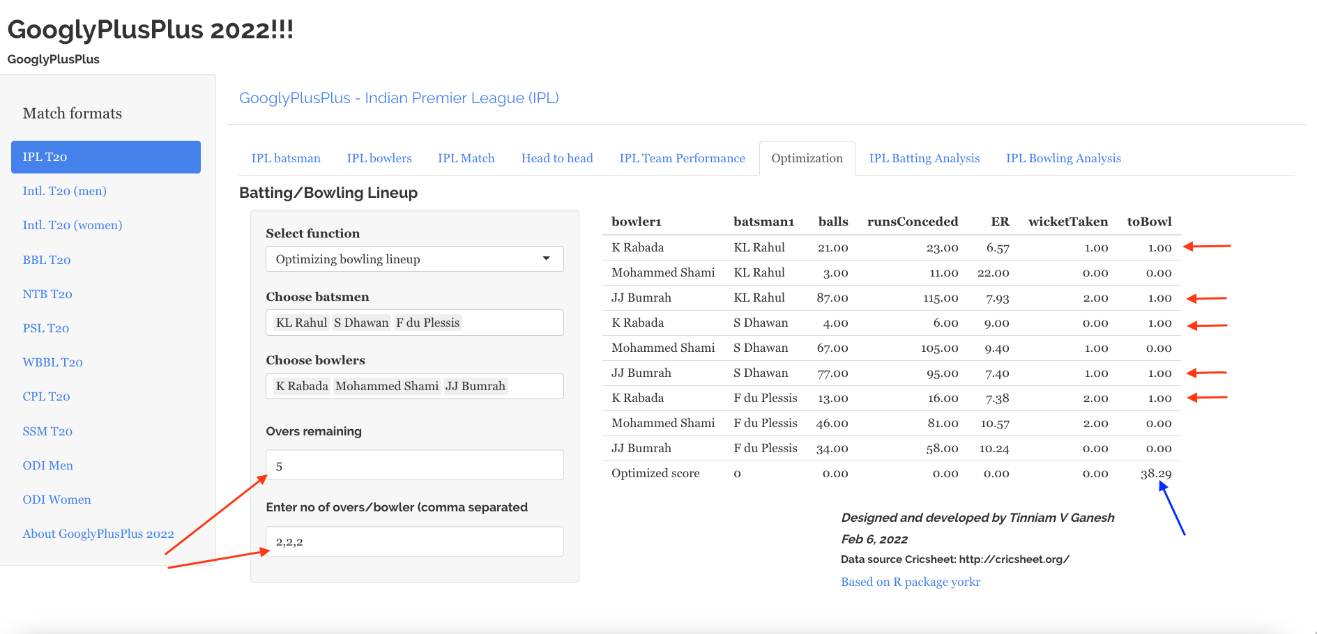
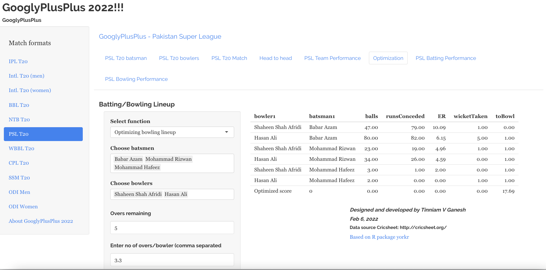
Let the economy rate $er_{ij}$ be the Economy Rate of the jth bowler to the ith batsman. Also if remaining overs for the bowlers are $o_{1},o_{2},o_{3}$
and the total number of overs left to be bowled are
$o_{1}+o_{2}+o_{3} = N$

Let the economy rate $er_{ij}$ be the Economy Rate of the jth bowler to the ith batsman.
Objective function : Minimize –
$er_{11}*o_{11} + er_{12}*o_{12} +..+er_{1n}*o_{1n}+ er_{21}*o_{21} + er_{22}*o_{22}+.. + er_{22}*o_{2n}+ er_{m1}*o_{m1}+..+ er_{mn}*o_{mn}$
i.e.
$\sum_{i=1}^{i=m}\sum_{j=1}^{i=n}er_{ij}*o_{ij}$
Constraints
Where $o_{j}$ is the number of overs remaining for the jth bowler against ‘k’ batsmen
$o_{j1} + o_{j2} + .. o_{jk} < o_{j}$
and if the total number of overs remaining to be bowled is N then
$o_{1} + o_{2} +...+ o_{k} = N$ or
$\sum_{j=1}^{j=k} o_{j} =N$
The overs that any bowler can bowl is $o_{j} >=0$

II) LP Formulation for batting lineup

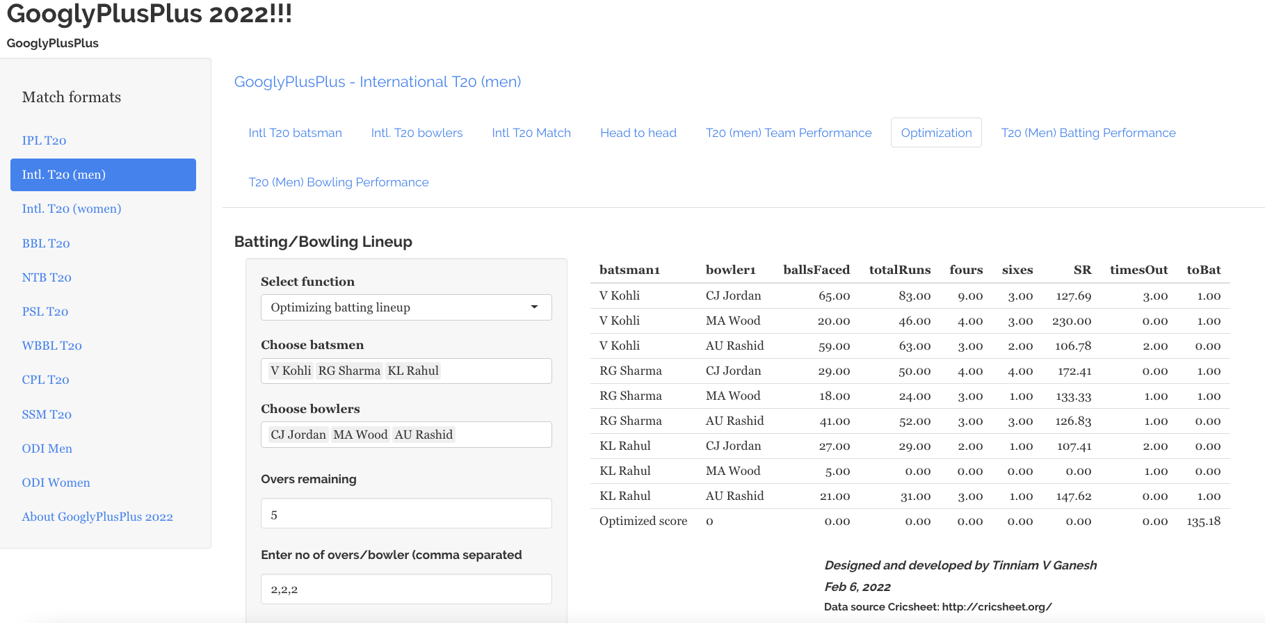
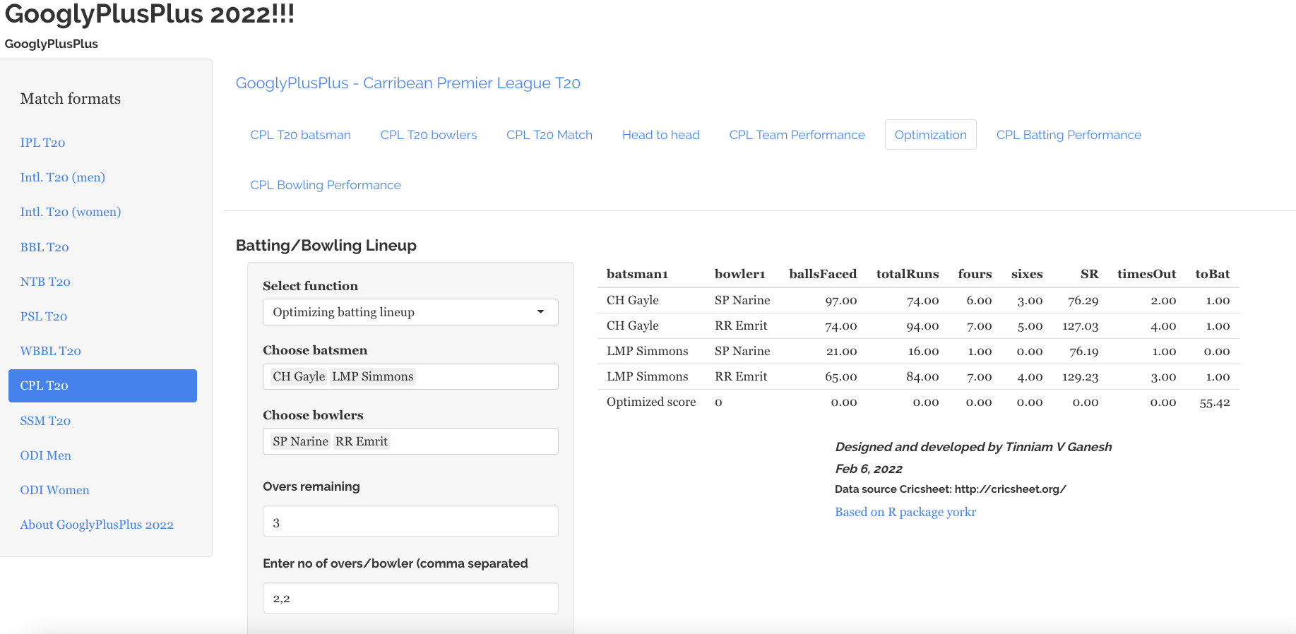
Let the strike rate $sr_{ij}$ be the Strike Rate of the ith batsman to the jth bowler
Objective function : Maximize –
$sr_{11}*o_{11} + sr_{12}*o_{12} +..+ sr_{1n}*o_{1n}+ sr_{21}*o_{21} + sr_{22}*o_{22}+.. sr_{2n}*o_{2n}+ sr_{m1}*o_{m1}+..+ sr_{mn}*o_{mn}$
i.e.
$\sum_{i=1}^{i=4}\sum_{j=1}^{i=3}sr_{ij}*o_{ij}$
Constraints
Where $o_{j}$ is the number of overs remaining for the jth bowler against ‘k’ batsmen
$o_{j1} + o_{j2} + .. o_{jk} < o_{j}$
and the total number of overs remaining to be bowled is N then
$o_{1} + o_{2} +...+ o_{k} = N$ or
$\sum_{j=1}^{j=k} o_{j} =N$
The overs that any bowler can bowl is
$o_{j} >=0$

C) Optimized bowling lineup

a) IPL – Optimizing bowling line up

Note: For computing the Optimal bowling lineup, the total number of overs remaining and the number of overs for each bowler have to be entered.

b) PSL – Optimizing batting line up

d) Optimized batting lineup

a) Intl. T20 (men) India vs England

b) Carribean Premier League – Optimizing batting line up

Give GooglyPlusPlus2022 a spin!

You can also check the code here gpp2022-1

Hope you have a good time with GooglyPlusPlus2022!

Also see

To see all posts click Index of posts

GooglyPlusPlus2021: Towards more picturesque analytics!

Analytics for e.g. sports analytics, business analytics or analytics in e-commerce or in other domain has 2 main requirements namely a) What kind of analytics (set of parameters,function) will squeeze out the most intelligence from the data b) How to represent the analytics so that an expert can garner maximum insight?

While it may appear that the former is more important, the latter is also equally, if not, more vital to the problem. Indeed, a picture is worth a thousand words, and often times is more insightful than a large table of numbers. However, in the case of sports analytics, for e.g. in cricket a batting or bowling scorecard captures more information and can never be represented in chart.

So, my Shiny app GooglyPlusPlus includes both charts and tables for different aspects of the analysis. In this post, a newer type of chart, popular among senior management experts, namely the 4 quadrant graph is introduced, which helps in categorising batsmen and bowlers into 4 categories as shown below

a) Batting Performances – Top right quadrant (High runs, High Strike rate)

b) Bowling Performances – Bottom right quadrant( High wickets, Low Economy Rate)

I have added the following 32 functions in this latest version of GooglyPlusPlus

A. Match Tab

All the functions below are at match level

Team Runs vs SR Plot
Team Wickets vs ER Plot
Team Runs vs SR Power play plot
Team Runs vs SR Middle overs plot
Team Runs vs SR Death overs plot
Team Wickets vs ER Power Play
Team Wickets vs ER Middle overs
Team Wickets vs ER Death overs

B. Head-to-head Tab

The below functions are based on all matches between 2 teams’

Team Runs vs SR Plot all Matches
Team Wickets vs ER Plot all Matches
Team Runs vs SR Power play plot all Matches
Team Runs vs SR Middle overs plot all Matches
Team Runs vs SR Death overs plot all Matches
Team Wickets vs ER Power Play plot all Matches
Team Wickets vs ER Middle overs plot all Matches
Team Wickets vs ER Death overs plot all Matches

C. Team Performance tab

The below functions are based on a team’s performance against all other teams

Team Runs vs SR Plot overall
Team Wickets vs ER Plot overall
Team Runs vs SR Power play plot overall
Team Runs vs SR Middle overs plot overall
Team Runs vs SR Death overs plot overall
Team Wickets vs ER Power Play overall
Team Wickets vs ER Middle overs overall
Team Wickets vs ER Death overs overall

D. T20 format Batting Analysis

This analysis is at T20 format level (IPL, Intl. T20(men), Intl. T20 (women), PSL, CPL etc.)

Overall Runs vs SR plot
Overall Runs vs SR Power play plot
Overall Runs vs SR Middle overs plot
Overall Runs vs SR Death overs plot

E. T20 Bowling Analysis

This analysis is at T20 format level (IPL, Intl. T20(men), Intl. T20 (women), PSL, CPL etc.)

Overall Wickets vs ER plot
Team Wickets vs ER Power Play
Team Wickets vs ER Middle overs
Team Wickets vs ER Death overs

These 32 functions have been added to my yorkr package and so all these functions become plug-n-play in my Shiny app GooglyPlusPlus2021 which means that the 32 functions apply across all the nine T20 formats that the app supports i.e. IPL, Intl. T20 (men), Intl. T20 (women), BBL, NTB, PSL, CPL, SSM, WBB.

Hence the multiplicative factor of the new addition is 32 x 9 = 288 additional ways of exploring match, team and player data

The data for GooglyPlusPlus is taken from Cricsheet. My shiny app GooglyPlusPlus2021 is based on my R package yorkr.

You can clone/fork GooglyPlusPlus from Github at gpp2021-10

Check out my app GooglyPlusPlus2021 and analyze batsmen, bowlers, teams, overall performance. The data for all the nine T20 formats have been updated to include the latest data.

Hence, the app is just in time for the IPL mega auction. You should be able to analyse players in IPL, Intl. T20 or in any of the other formats from where they could be drawn and check out their relative standings

I am including some random plots to demonstrate the newly minted functions

Note 1: All plots are interactive. The controls are on the top right. You can hover over data, zoom-in, zoom-out, compare data etc by choosing the appropriate control. To know more about how to use the interactive charts see GooglyPlusPlus2021 is now fully interactive!!!

You can also check my short video on how to navigate interactive charts

Note 2: To know about Powerplay, Middle overs and Death over analysis see my post GooglyPlusPlus2021 now with power play, middle and death over analysis

Note 3: All tabs(except Match tab) now include Date range pickers to focus on the period of interest. See my post GooglyPlusPlus2021 enhanced with drill-down batsman, bowler analytics

I) Match tab

New Zealand vs Australia (2021-11-14)

New Zealand batting, except K Williamson, the rest did not fire as much

For Australia, Warner, Maxwell and Marsh played good knocks to wrest control

II) Head-to-head

a) Wickets vs ER during Power play of Mumbai Indians in all matches against Chennai Super Kings (IPL)

b) Karachi Kings Runs vs SR during middle overs against Multan Sultans (PSL)

c) Wickets vs ER during death overs of Barbados Tridents in all matches against Jamaica Tallawahs (CPL)

III) Teams overall batting performance

India’s best T20 performers in Power play since 2018 (Intl. T20)

e) Australia’s best performers in Death overs since Mar 2017 (Intl. T20)

f) India’s Intl. T20 (women) best Runs vs SR since 2018

g) England’s Intl. T20 (women) best bowlers in Death overs

IV) Overall Batting Performance across T20

This tab gives the batsmen’s rank and overall batting performance across the T20 format.

a) Why was Hardik Pandya chosen, and why this was in error?

Of course, it provides an insight into why Hardik Pandya was chosen in India’s World cup team despite poor performances recently. Here are the best Intl. T20 death over batsmen