Image classification using Deep Learning has been around for almost a decade. In fact, this field with the use of Convolutional Neural Networks (CNN) is quite mature and the algorithms work very well in image classification, object detection, facial recognition and self-driving cars. In this post, I use AI image classification to identify cricketing shots. While the problem falls in a well known domain, the application of image classification in identifying cricketing shots is probably new. I have selected three cricketing shots, namely, the front drive, sweep shot, and the hook shot for this purpose. My purpose was to build a proof-of-concept and not a perfect product. I have kept the dataset deliberately small (for obvious reasons) of just about 14 samples for each cricketing shot, and for a total of about 41 total samples for both training and test data. Anyway, I get a reasonable performance from the AI model.
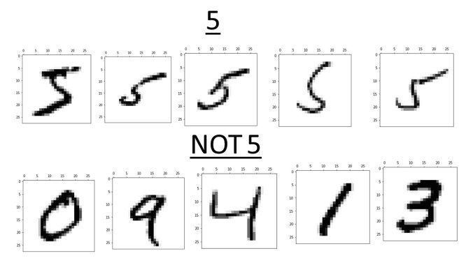
Included below are some examples of the data set
This post is based on this or on Image classification from Hugging face. Interestingly, this, the model used here is based on Vision Transformers (ViT from Google Brain) and not on Convolutional Neural Networks as is usually done.
The steps are to fine-tune ViT Transformer with the ‘strokes’ dataset are
d) Create a dictionary that maps the label name to an integer and vice versa. Display the labels
labels = df1.features["label"].names
label2id, id2label = dict(), dict()
for i, label in enumerate(labels):
label2id[label] = str(i)
id2label[str(i)] = label
labels
['front drive', 'hook shot', 'sweep shot']
e) Load ViT image processor. To apply the correct transformations, ImageProcessor is initialised with a configuration that was saved along with the pretrained model
from transformers import AutoImageProcessor
checkpoint = "google/vit-base-patch16-224-in21k"
image_processor = AutoImageProcessor.from_pretrained(checkpoint)
f) Apply image transformations to the images to make the model more robust against overfitting
from torchvision.transforms import RandomResizedCrop, Compose, Normalize, ToTensor
normalize = Normalize(mean=image_processor.image_mean, std=image_processor.image_std)
size = (
image_processor.size["shortest_edge"]
if "shortest_edge" in image_processor.size
else (image_processor.size["height"], image_processor.size["width"])
)
_transforms = Compose([RandomResizedCrop(size), ToTensor(), normalize])
g) Create a preprocessing function to apply the transforms and return pixel_values of the image as the inputs to the model – :
def transforms(examples):
examples["pixel_values"] = [_transforms(img.convert("RGB")) for img in examples["image"]]
del examples["image"]
return examples
h) Apply the preprocessing function over the entire dataset, using Hugging Face Dataset’s ‘with_transform’ method
df1 = df1.with_transform(transforms)
from transformers import DefaultDataCollator
data_collator = DefaultDataCollator()
As I mentioned before, the model should be reasonably accurate but not perfect, since my training dataset is extremely small. This is just a prototype to show that shot identification in cricket with AI is in the realm of the possible.
Ever since I started to use ChatGPT, I have been fascinated by its capabilities. To a large extent, the abilities of Large Language Models (LLMs) is quite magical – the way it answers questions, the way it summarises passages, the way it creates poems et cetera. All the LLMs need is a large corpus of data from the internet, articles, wikis, blogs, and so on.
On delving a little deeper into Generative AI, LLMs I learnt that, this is based on the principle of being able to predict the most probable word in a given sequence. It made me wonder whether the world of ideas, language and communication are actually governed by probabilities. Does what we communicate fall within the purview of statistics?
As an aside, just by extending further if we visualise a world in which every human action to a situation is assigned an embedding vector, and if we feed the responses of all humans over time in different situations, to the equivalent of a Transformer of a Large Human Reaction Model (LHRM) ;-), we can envisage the model being capable of predicting the response of human in a given situation. In my opinion, the machine would be fairly right most of the occasions as it could select the most probable choice of action, much like ‘The Machine’ in Person of Interest. However, this does not mean that the machine (AI) is actually more intelligent than humans. All it means is that the choice of humans responses are a part of a finite subset possibilities and The Machine (AI) can compute the possibilities and associated probabilities much quicker than humans. Does it mean that the world is deterministic? Possibly.
In this post, I use the T5 transformer to summarise Indian philosophy. For this task, I have fine-tuned the T5 model with a curated dataset taken from random passages on Hindu philosophy available on the internet. For each passage, I had to and hand-create the corresponding summary. This was a fairly tedious and demanding task but an enlightening one. It was interesting to understand how our ancestors, the Rishis, understood reality, the physical world, senses, the mind, the intellect, consciousness (Atman) and universal consciousness (Brahman). (Incidentally I was only able to curate only about 130 rows of philosophical snippets and manually create the corresponding summaries. Probably this is a very small dataset for fine-tuning but I just wanted to see the performance of the T5 model in a new domain.)
In this post the T5 model is fine-tuned with the curated dataset and the rouge1 and rouge2 scores are used to evaluate the model’s performance.
I have used the Hugging Face Hub for the transformer model, corresponding LLM functions and management of the dataset etc. The Hugging Face ecosystem is simply wow!!
 from huggingface_hub import notebook_login
notebook_login()

Login successful
c) Load the curated dataset on Hindu philosophy
from datasets import load_dataset
df1 = load_dataset("tvganesh/philosophy",split='train')
d) Load a T5 tokenizer to process text and summary
Prefix the input with a prompt so T5 knows this is a summarization task.
Use the keyword text_target argument when tokenizing labels.
Truncate sequences to be no longer than the maximum length set by the max_length parameter. The max_length of the text kept at 220 words and the max_length of the summary is kept at 50 words.
The ‘map’ function of the Huggingface dataset can be used to apply the pre_process function across the entire data.
DataCollatorForSeq2Seq can be used to dynamically pad the sentences to the longest length in a batch during collation, instead of padding the whole dataset to the maximum length.
from transformers import DataCollatorForSeq2Seq
data_collator = DataCollatorForSeq2Seq(tokenizer=tokenizer, model=checkpoint)
e) Evaluate performance of Model
The rouge1,rouge2 metric can be used to evaluate the performance of the model
import evaluate
rouge = evaluate.load("rouge")
f)Create a function compute_metrics that passes your predictions and labels to ‘compute’ to calculate the ROUGE metric:
import numpy as np

def compute_metrics(eval_pred):
    # evaluate predictions and labels
    predictions, labels = eval_pred
    decoded_preds = tokenizer.batch_decode(predictions, skip_special_tokens=True)
    labels = np.where(labels != -100, labels, tokenizer.pad_token_id)
    decoded_labels = tokenizer.batch_decode(labels, skip_special_tokens=True)
     # compute rouge score between the labels and predictions
    result = rouge.compute(predictions=decoded_preds, references=decoded_labels, use_stemmer=True)

    prediction_lens = [np.count_nonzero(pred != tokenizer.pad_token_id) for pred in predictions]
    result["gen_len"] = np.mean(prediction_lens)

    return {k: round(v, 4) for k, v in result.items()}
g) Split the data into training(80%) and test(20%) data set
from transformers import AutoModelForSeq2SeqLM, Seq2SeqTrainingArguments, Seq2SeqTrainer
model = AutoModelForSeq2SeqLM.from_pretrained(checkpoint)
i)
Set training hyperparameters in Seq2SeqTrainingArguments. The Adam optimization, with learning rate, beta1 & beta2 are used
Pass the training arguments to Seq2SeqTrainer along with the model, dataset, tokenizer, data collator, and compute_metrics function.
Call train() to finetune your model.
training_args = Seq2SeqTrainingArguments(
    output_dir="philosophy_model",
    evaluation_strategy="epoch",
    learning_rate= 5.6e-03,
    adam_beta1=0.9,
    adam_beta2=0.99,
    adam_epsilon=1e-06,
    per_device_train_batch_size=8,
    per_device_eval_batch_size=8,
    weight_decay=0.01,
    save_total_limit=3,
    num_train_epochs=20,
    predict_with_generate=True,
    fp16=True,
    push_to_hub=True,
)

trainer = Seq2SeqTrainer(
    model=model,
    args=training_args,
    train_dataset=train_dataset,
    eval_dataset=test_dataset,
    tokenizer=tokenizer,
    data_collator=data_collator,
    compute_metrics=compute_metrics,
)

trainer.train()

Epoch	Training Loss	Validation Loss	Rouge1	Rouge2	Rougel	Rougelsum	Gen Len
1	No log	2.246223	0.363200	0.146200	0.311400	0.312600	18.333300
2	No log	1.461140	0.459000	0.303900	0.417800	0.417800	18.566700
3	No log	0.832312	0.546500	0.425900	0.524700	0.520800	17.133300
4	No log	0.472341	0.616100	0.517600	0.601000	0.600400	18.366700
5	No log	0.312106	0.681200	0.607800	0.674700	0.671400	18.233300
6	No log	0.154585	0.741800	0.702300	0.733800	0.731300	18.066700
7	No log	0.112100	0.783200	0.763000	0.780200	0.778900	18.500000
8	No log	0.069882	0.801400	0.788200	0.802700	0.800900	18.533300
9	No log	0.045941	0.795800	0.780500	0.794600	0.791700	18.500000
10	No log	0.051655	0.809100	0.795800	0.810500	0.809000	18.466700
11	No log	0.035792	0.799400	0.785200	0.797300	0.794600	18.500000
12	No log	0.041766	0.779900	0.754800	0.774700	0.773200	18.266700
13	No log	0.010703	0.810000	0.800400	0.810700	0.809000	18.500000
14	No log	0.006519	0.807700	0.797100	0.809400	0.807500	18.500000
15	No log	0.017779	0.808000	0.796000	0.809400	0.807500	18.366700
16	No log	0.001681	0.810000	0.800400	0.810700	0.809000	18.500000
17	No log	0.005469	0.810000	0.800400	0.810700	0.809000	18.500000
18	No log	0.002003	0.810000	0.800400	0.810700	0.809000	18.500000
19	No log	0.000638	0.810000	0.800400	0.810700	0.809000	18.500000
20	No log	0.000498	0.810000	0.800400	0.810700	0.809000	18.500000
TrainOutput(global_step=260, training_loss=0.6491916949932391, metrics={'train_runtime': 57.99, 'train_samples_per_second': 34.489, 'train_steps_per_second': 4.484, 'total_flos': 101132046434304.0, 'train_loss': 0.6491916949932391, 'epoch': 20.0})
As we can see the rouge1 to rouge2 scores are fairly good. Anything above 0.5 is considered good. Maybe this is because the T5 model has already been pre-trained on a fairly large philosophical dataset
j) Push to hub
trainer.push_to_hub()
k) Summarise using pipeline
text = "summarize: A seeker who has the necessary qualifications, in order that he may be redeemed from his inner weaknesses, attachments, animalisms and false values is advised to serve with devotion a Teacher who is well- established in the experience of the Self."

from transformers import pipeline

summarizer = pipeline("summarization", model="tvganesh/philosophy_model")
summarizer(text)

[{'summary_text': 'A seeker who has the necessary qualifications will be able to free oneself of sense objects, and one cannot expect this to happen without any mental tossing'}]
l) Summarise using model generate
from transformers import AutoTokenizer

tokenizer = AutoTokenizer.from_pretrained("tvganesh/philosophy_model")
inputs = tokenizer(text, return_tensors="pt").input_ids

from transformers import AutoModelForSeq2SeqLM

model = AutoModelForSeq2SeqLM.from_pretrained("tvganesh/philosophy_model")
outputs = model.generate(inputs, max_new_tokens=70, do_sample=False)

tokenizer.decode(outputs[0], skip_special_tokens=True)

'A seeker who has the necessary qualifications will help in his journey to redeem himself'
l) Number of beams
summary_ids = model.generate(inputs,
                                    num_beams=10,
                                    no_repeat_ngram_size=3,
                                    min_length=20,
                                    max_length=70,
                                    early_stopping=True)
output = tokenizer.decode(summary_ids[0], skip_special_tokens=True)
output

'A seeker who has the necessary qualifications will be able to free himself of sense objects and false values'
I also tried Facebook’s BART Large model but the performance was not good at all.
You can try out the model at the following link philosophy_model
This should be my last post on computing T20 Win Probability. In this post I compute Win Probability using Augmented Data with the help of Conditional Tabular Generative Adversarial Networks (CTGANs).
A.Introduction
I started the computation of T20 match Win Probability in my earlier post
This was lightweight and could be easily deployed in my Shiny GooglyPlusPlus app as opposed to the Tidymodel’s Random Forest, which was bulky and slow.
d) Finally I decided to try and improve the accuracy of my Deep Learning Model using Synthetic data. Towards this end, my explorations led me to Conditional Tabular Generative Adversarial Networks (CTGANs). CTGAN are GAN networks that can be used with Tabular data as GAN models are not useful with tabular data. However, the best performance I got for
DL Keras Model + Synthetic data : accuracy =0.77
The poorer accuracy was because CTGAN requires enormous computing power (GPUs) and RAM. The free version of Colab, Kaggle kept crashing when I tried with even 0.1 % of my 1.2 million dataset size. Finally, I tried with just 0.05% and was able to generate synthetic data. Most likely, it is the small sample size and the smaller number of epochs could be the reason for the poor result. In any case, it was worth trying and this approach would possibly work with sufficient computing resources.
B.Generative Adversarial Networks (GANs)
Generative Adversarial Networks (GANs) was the brain child of Ian Goodfellow who demonstrated it in 2014. GANs are capable of generating synthetic text, tables, images, videos using available data. In Adversarial nets framework, the generative model is pitted against an adversary: a discriminative model that learns to determine whether a sample is from the model distribution or the data distribution.
GANs have 2 Deep Neural Networks , the Generator and Discriminator which compete against other
The Generator (Counterfeiter) takes random noise as input and generates fake images, tables, text. The generator learns to generate plausible data. The generated instances become negative training examples for the discriminator.
The Discriminator (Police) which tries to distinguish between the real and fake images, text. The discriminator learns to distinguish the generator’s fake data from real data. The discriminator penalises the generator for producing implausible results.
A pictorial representation of the GAN model can be shown below
Theoretically best performance of GANs are supposed to happen when the network reaches the ‘Nash equilibrium‘, i.e. when the Generator produces near fake images and the Discriminator’s loss is f ~0.5 i.e. the discriminator is unable to distinguish between real and fake images.
Note: Though I have mentioned T20 data in the above GAN model, the T20 tabular data is actually used in CTGAN which is slightly different from the above. See Reference 2) below.
C. Conditional Tabular Generative Adversial Networks (CTGANs)
“Modeling the probability distribution of rows in tabular data and generating realistic synthetic data is a non-trivial task. Tabular data usually contains a mix of discrete and continuous columns. Continuous columns may have multiple modes whereas discrete columns are sometimes imbalanced making the modeling difficult.” CTGANs handle these challenges.
I came upon CTGAN after spending some time exploring GANs via blogs, videos etc. For building the model I use real T20 match data. However, CTGAN requires immense raw computing power and a lot of RAM. My initial attempts on Colab, my Mac (12 core, 32GB RAM), took forever before eventually crashing, I switched to Kaggle and used GPUs. Still I was only able to use only a miniscule part of my T20 dataset. My match data has 1.2 million rows, hoanything > 0.05% resulted in Kaggle crashing. Since I was able to use only a fraction, I executed the CTGAN model over several iterations, each iteration with a random 0.05% sample of the dataset. At the end of each iterations I also generate synthetic dataset. Over 12 iterations, I generate close 360K of ‘synthetic‘ T20 match data.
I then augment the 1.2 million rows of ‘real‘ T20 match data with the generated ‘synthetic T20 match data to run my Deep Learning model
Here the quality of the synthetic data set is evaluated.
a) Statistical evaluation
Read the real T20 match data
Read the generated T20 synthetic match data
import pandas as pd

# Read the T20 match and synthetic match data
df = pd.read_csv('/kaggle/input/cricket1/t20.csv').  #1.2 million rows
synthetic=pd.read_csv('/kaggle/input/synthetic/synthetic.csv')   #300K

# Randomly sample 1000 rows, and generate stats
df1=df.sample(n=1000)
real=df1.describe()
realData_stats=real.transpose
print(realData_stats)

synthetic1=synthetic.sample(n=1000)
synthetic=synthetic1.describe()
syntheticData_stats=synthetic.transpose
syntheticData_stats
import pandas as pd

# CTGAN prints out a new line for each epoch
epochs_output = str(output).split('\n')

# CTGAN separates the values with commas
raw_values = [line.split(',') for line in epochs_output]
loss_values = pd.DataFrame(raw_values)[:-1] # convert to df and delete last row (empty)

# Rename columns
loss_values.columns = ['Epoch', 'Generator Loss', 'Discriminator Loss']

# Extract the numbers from each column
loss_values['Epoch'] = loss_values['Epoch'].str.extract('(\d+)').astype(int)
loss_values['Generator Loss'] = loss_values['Generator Loss'].str.extract('([-+]?\d*\.\d+|\d+)').astype(float)
loss_values['Discriminator Loss'] = loss_values['Discriminator Loss'].str.extract('([-+]?\d*\.\d+|\d+)').astype(float)

# the result is a row for each epoch that contains the generator and discriminator loss
loss_values.head()
import plotly.graph_objects as go

# Plot loss function
fig = go.Figure(data=[go.Scatter(x=loss_values['Epoch'], y=loss_values['Generator Loss'], name='Generator Loss'),
                      go.Scatter(x=loss_values['Epoch'], y=loss_values['Discriminator Loss'], name='Discriminator Loss')])


# Update the layout for best viewing
fig.update_layout(template='plotly_white',
                    legend_orientation="h",
                    legend=dict(x=0, y=1.1))

title = 'CTGAN loss function for T20 dataset - '
fig.update_layout(title=title, xaxis_title='Epoch', yaxis_title='Loss')
fig.show()
G. Qualitative evaluation of Synthetic data
a) Quality of continuous columns in synthetic data
KSComplement -This metric computes the similarity of a real column vs. a synthetic column in terms of the column shapes.The KSComplement uses the Kolmogorov-Smirnov statistic. Closer to 1.0 is good and 0 is worst
The performance is decent but not excellent. I was unable to execute more epochs as it it required larger than the memory allowed
c) Correlation similarity
This metric measures the correlation between a pair of numerical columns and computes the similarity between the real and synthetic data – it compares the trends of 2D distributions. Best 1.0 and 0.0 is worst
In this final part I augment my T20 match data set with the generated synthetic T20 data set.
import pandas as pd
from numpy import savetxt
import tensorflow as tf
from tensorflow import keras
import pandas as pd
import numpy as np


from keras.layers import Input, Embedding, Flatten, Dense, Reshape, Concatenate, Dropout
from keras.models import Model
import matplotlib.pyplot as plt

# Read real and synthetic data
df = pd.read_csv('/kaggle/input/cricket1/t20.csv')
synthetic=pd.read_csv('/kaggle/input/synthetic/synthetic.csv')

# Augment the data. Concatenate real & synthetic data
df1=pd.concat([df,synthetic])

# Create training and test samples
print("Shape of dataframe=",df1.shape)
train_dataset = df1.sample(frac=0.8,random_state=0)
test_dataset = df1.drop(train_dataset.index)
train_dataset1 = train_dataset[['batsmanIdx','bowlerIdx','ballNum','ballsRemaining','runs','runRate','numWickets','runsMomentum','perfIndex']]
test_dataset1 = test_dataset[['batsmanIdx','bowlerIdx','ballNum','ballsRemaining','runs','runRate','numWickets','runsMomentum','perfIndex']]
train_dataset1
train_labels = train_dataset.pop('isWinner')
test_labels = test_dataset.pop('isWinner')
print(train_dataset1.shape)

a=train_dataset1.describe()
stats=a.transpose
print(a)
As can be seen the accuracy with augmented dataset is around 0.77, while without it I was getting 0.867 with just the real data. This degradation is probably due to the folllowing reasons
Only a fraction of the dataset was used for training. This was not representative of the data distribution for CTGAN to correctly synthesise data
The number of epochs had to be kept low to prevent Kaggle/Colab from crashing
I. Conclusion
This post shows how we can generate synthetic T20 match data to augment real T20 match data. Assuming we have sufficient processing power we should be able to generate synthetic data for augmenting our data set. This should improve the accuracy of the Win Probabily Deep Learning model.
Often times before crucial matches, or in general, we would like to know the performance of a batsman against a bowler or vice-versa, but we may not have the data. We generally have data where different batsmen would have faced different sets of bowlers with certain performance data like ballsFaced, totalRuns, fours, sixes, strike rate and timesOut. Similarly different bowlers would have performance figures(deliveries, runsConceded, economyRate and wicketTaken) against different sets of batsmen. We will never have the data for all batsmen against all bowlers. However, it would be good estimate the performance of batsmen against a bowler, even though we do not have the performance data. This could be done using collaborative filtering which identifies and computes based on the similarity between batsmen vs bowlers & bowlers vs batsmen.
This post shows an approach whereby we can estimate a batsman’s performance against bowlers even though the batsman may not have faced those bowlers, based on his/her performance against other bowlers. It also estimates the performance of bowlers against batsmen using the same approach. This is based on the recommender algorithm which is used to recommend products to customers based on their rating on other products.
This idea came to me while generating the performance of batsmen vs bowlers & vice-versa for 2 IPL teams in this IPL 2022 with my Shiny app GooglyPlusPlus in the optimization tab, I found that there were some batsmen for which there was no data against certain bowlers, probably because they are playing for the first time in their team or because they were new (see picture below)
In the picture above there is no data for Dewald Brevis against Jasprit Bumrah and YS Chahal. Wouldn’t be great to estimate the performance of Brevis against Bumrah or vice-versa? Can we estimate this performance?
While pondering on this problem, I realized that this problem formulation is similar to the problem formulation for the famous Netflix movie recommendation problem, in which user’s ratings for certain movies are known and based on these ratings, the recommender engine can generate ratings for movies not yet seen.
This post estimates a player’s (batsman/bowler) using the recommender engine This post is based on R package recommenderlab
You can download this R Markdown file and the associated data and perform the analysis yourself using any other recommender engine from Github at playerPerformanceEstimation
Problem statement
In the table below we see a set of bowlers vs a set of batsmen and the number of times the bowlers got these batsmen out. By knowing the performance of the bowlers against some of the batsmen we can use collaborative filter to determine the missing values. This is done using the recommender engine.
The Recommender Engine works as follows. Let us say that there are feature vectors , and for the 3 bowlers which identify the characteristics of these bowlers (“fast”, “lateral drift through the air”, “movement off the pitch”). Let each batsman be identified by parameter vectors , and so on
For e.g. consider the following table
Then by assuming an initial estimate for the parameter vector and the feature vector xx we can formulate this as an optimization problem which tries to minimize the error for This can work very well as the algorithm can determine features which cannot be captured. So for e.g. some particular bowler may have very impressive figures. This could be due to some aspect of the bowling which cannot be captured by the data for e.g. let’s say the bowler uses the ‘scrambled seam’ when he is most effective, with a slightly different arc to the flight. Though the algorithm cannot identify the feature as we know it, but the ML algorithm should pick up intricacies which cannot be captured in data.
Hence the algorithm can be quite effective.
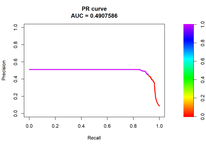
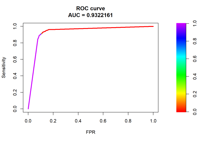
Note: The recommender lab performance is not very good and the Mean Square Error is quite high. Also, the ROC and AUC curves show that not in aLL cases the algorithm is doing a clean job of separating the True positives (TPR) from the False Positives (FPR)
Note: This is similar to the recommendation problem
The collaborative optimization object can be considered as a minimization of both and the features x and can be written as
J(, }= 1/2
The collaborative filtering algorithm can be summarized as follows
Initialize , … and the set of features be ,, … , to small random values
Minimize J(, … ,, , … ,) using gradient descent. For every j=1,2, …, i= 1,2,..,
:= – ( ) –
&
:= – (
Hence for a batsman with parameters and a bowler with (learned) features x, predict the “times out” for the player where the value is not known using
The above derivation for the recommender problem is taken from Machine Learning by Prof Andrew Ng at Coursera from the lecture Collaborative filtering
There are 2 main types of Collaborative Filtering(CF) approaches
User based Collaborative Filtering User-based CF is a memory-based algorithm which tries to mimics word-of-mouth by analyzing rating data from many individuals. The assumption is that users with similar preferences will rate items similarly.
Item based Collaborative Filtering Item-based CF is a model-based approach which produces recommendations based on the relationship between items inferred from the rating matrix. The assumption behind this approach is that users will prefer items that are similar to other items they like.
1a. A note on ROC and Precision-Recall curves
A small note on interpreting ROC & Precision-Recall curves in the post below
ROC Curve: The ROC curve plots the True Positive Rate (TPR) against the False Positive Rate (FPR). Ideally the TPR should increase faster than the FPR and the AUC (area under the curve) should be close to 1
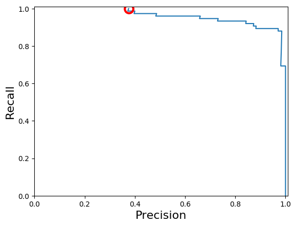
Precision-Recall: The precision-recall curve shows the tradeoff between precision and recall for different threshold. A high area under the curve represents both high recall and high precision, where high precision relates to a low false positive rate, and high recall relates to a low false negative rate
Helper functions for the RMarkdown notebook are created
eval – Gives details of RMSE, MSE and MAE of ML algorithm
evalRecomMethods – Evaluates different recommender methods and plot the ROC and Precision-Recall curves
# This function returns the error for the chosen algorithm and also predicts the estimates
# for the given data
eval <- function(data, train1, k1,given1,goodRating1,recomType1="UBCF"){
  set.seed(2022)
  e<- evaluationScheme(data,
                       method = "split",
                       train = train1,
                       k = k1,
                       given = given1,
                       goodRating = goodRating1)

  r1 <- Recommender(getData(e, "train"), recomType1)
  print(r1)

  p1 <- predict(r1, getData(e, "known"), type="ratings")
  print(p1)

  error = calcPredictionAccuracy(p1, getData(e, "unknown"))

  print(error)
  p2 <- predict(r1, data, type="ratingMatrix")
  p2
}
# This function will evaluate the different recommender algorithms and plot the AUC and ROC curves
evalRecomMethods <- function(data,k1,given1,goodRating1){
  set.seed(2022)
  e<- evaluationScheme(data,
                       method = "cross",
                       k = k1,
                       given = given1,
                       goodRating = goodRating1)

  models_to_evaluate <- list(
    `IBCF Cosinus` = list(name = "IBCF",
                          param = list(method = "cosine")),
    `IBCF Pearson` = list(name = "IBCF",
                          param = list(method = "pearson")),
    `UBCF Cosinus` = list(name = "UBCF",
                          param = list(method = "cosine")),
    `UBCF Pearson` = list(name = "UBCF",
                          param = list(method = "pearson")),
    `Zufälliger Vorschlag` = list(name = "RANDOM", param=NULL)
  )

  n_recommendations <- c(1, 5, seq(10, 100, 10))
  list_results <- evaluate(x = e,
                           method = models_to_evaluate,
                           n = n_recommendations)
  plot(list_results, annotate=c(1,3), legend="bottomright")
  plot(list_results, "prec/rec", annotate=3, legend="topleft")
}
3. Batsman performance estimation
The section below regenerates the performance for batsmen based on incomplete data for the different fields in the data frame namely balls faced, fours, sixes, strike rate, times out. The recommender lab allows one to test several different algorithms all at once namely
User based – Cosine similarity method, Pearson similarity
Item based – Cosine similarity method, Pearson similarity
Popular
Random
SVD and a few others
3a. Batting dataframe
head(df)
##   batsman1         bowler1 ballsFaced totalRuns fours sixes  SR timesOut
## 1 A Badoni        A Mishra          0         0     0     0 NaN        0
## 2 A Badoni        A Nortje          0         0     0     0 NaN        0
## 3 A Badoni         A Zampa          0         0     0     0 NaN        0
## 4 A Badoni     Abdul Samad          0         0     0     0 NaN        0
## 5 A Badoni Abhishek Sharma          0         0     0     0 NaN        0
## 6 A Badoni      AD Russell          0         0     0     0 NaN        0
3b Data set and data preparation
For this analysis the data from Cricsheet has been processed using my R package yorkr to obtain the following 2 data sets – batsmenVsBowler – This dataset will contain the performance of the batsmen against the bowler and will capture a) ballsFaced b) totalRuns c) Fours d) Sixes e) SR f) timesOut – bowlerVsBatsmen – This data set will contain the performance of the bowler against the difference batsmen and will include a) deliveries b) runsConceded c) EconomyRate d) wicketsTaken
Obviously many rows/columns will be empty
This is a large data set and hence I have filtered for the period > Jan 2020 and < Dec 2022 which gives 2 datasets a) batsmanVsBowler20_22.rdata b) bowlerVsBatsman20_22.rdata
I also have 2 other datasets of all batsmen and bowlers in these 2 dataset in the files c) all-batsmen20_22.rds d) all-bowlers20_22.rds
##                 A Mishra A Nortje A Zampa Abdul Samad Abhishek Sharma
## A Badoni              NA       NA      NA          NA              NA
## A Manohar             NA       NA      NA          NA              NA
## A Nortje              NA       NA      NA          NA              NA
## AB de Villiers        NA        4       3          NA              NA
## Abdul Samad           NA       NA      NA          NA              NA
## Abhishek Sharma       NA       NA      NA          NA              NA
## AD Russell             1       NA      NA          NA              NA
## AF Milne              NA       NA      NA          NA              NA
## AJ Finch              NA       NA      NA          NA               3
## AJ Tye                NA       NA      NA          NA              NA
##                 AD Russell AF Milne AJ Tye AK Markram Akash Deep
## A Badoni                NA       NA     NA         NA         NA
## A Manohar               NA       NA     NA         NA         NA
## A Nortje                NA       NA     NA         NA         NA
## AB de Villiers           3       NA      3         NA         NA
## Abdul Samad             NA       NA     NA         NA         NA
## Abhishek Sharma         NA       NA     NA         NA         NA
## AD Russell              NA       NA      6         NA         NA
## AF Milne                NA       NA     NA         NA         NA
## AJ Finch                NA       NA     NA         NA         NA
## AJ Tye                  NA       NA     NA         NA         NA
The dots below represent data for which there is no performance data. These cells need to be estimated by the algorithm
set.seed(2022)
r <- as(df8,"realRatingMatrix")
getRatingMatrix(r)[1:15,1:15]
## 15 x 15 sparse Matrix of class "dgCMatrix"
## [[ suppressing 15 column names 'A Mishra', 'A Nortje', 'A Zampa' ... ]]
The data frame of the batsman vs bowlers from the period 2020 -2022 is read as a dataframe. To remove rows with very low number of ratings(timesOut, SR, Fours, Sixes etc), the rows are filtered so that there are at least more 10 values in the row. For the player estimation the dataframe is converted into a wide-format as a matrix (m x n) of batsman x bowler with each of the columns of the dataframe i.e. timesOut, SR, fours or sixes. These different matrices can be considered as a rating matrix for estimation.
A similar approach is taken for estimating bowler performance. Here a wide form matrix (m x n) of bowler x batsman is created for each of the columns of deliveries, runsConceded, ER, wicketsTaken
5. Batsman’s times Out
The code below estimates the number of times the batsmen would lose his/her wicket to the bowler. As discussed in the algorithm above, the recommendation engine will make an initial estimate features for the bowler and an initial estimate for the parameter vector for the batsmen. Then using gradient descent the recommender engine will determine the feature and parameter values such that the over Mean Squared Error is minimum
From the plot for the different algorithms it can be seen that UBCF performs the best. However the AUC & ROC curves are not optimal and the AUC> 0.5
df3 <- select(df, batsman1,bowler1,timesOut)
df6 <- xtabs(timesOut ~ ., df3)
df7 <- as.data.frame.matrix(df6)
df8 <- data.matrix(df7)
df8[df8 == 0] <- NA
r <- as(df8,"realRatingMatrix")
# Filter only rows where the row count is > 10
r0=r[(rowCounts(r) > 10),]
getRatingMatrix(r0)[1:10,1:10]
## 10 x 10 sparse Matrix of class "dgCMatrix"
## [[ suppressing 10 column names 'A Mishra', 'A Nortje', 'A Zampa' ... ]]
##    Min. 1st Qu.  Median    Mean 3rd Qu.    Max.
##   1.000   3.000   3.000   3.463   4.000  21.000
# Evaluate the different plotting methods
evalRecomMethods(r0[1:dim(r0)[1]],k1=5,given=7,goodRating1=median(getRatings(r0)))
#Evaluate the error
a=eval(r0[1:dim(r0)[1]],0.8,k1=5,given1=7,goodRating1=median(getRatings(r0)),"UBCF")
## Recommender of type 'UBCF' for 'realRatingMatrix'
## learned using 70 users.
## 18 x 145 rating matrix of class 'realRatingMatrix' with 1755 ratings.
##     RMSE      MSE      MAE
## 2.069027 4.280872 1.496388
b=round(as(a,"matrix")[1:10,1:10])
c <- as(b,"realRatingMatrix")
m=as(c,"data.frame")
names(m) =c("batsman","bowler","TimesOut")
6. Batsman’s Strike rate
This section deals with the Strike rate of batsmen versus bowlers and estimates the values for those where the data is incomplete using UBCF method.
Even here all the algorithms do not perform too efficiently. I did try out a few variations but could not lower the error (suggestions welcome!!)
## Recommender of type 'UBCF' for 'realRatingMatrix'
## learned using 105 users.
## 27 x 145 rating matrix of class 'realRatingMatrix' with 3220 ratings.
##       RMSE        MSE        MAE
##   77.71979 6040.36508   58.58484
b=round(as(a,"matrix")[1:10,1:10])
c <- as(b,"realRatingMatrix")
n=as(c,"data.frame")
names(n) =c("batsman","bowler","SR")
7. Batsman’s Sixes
The snippet of code estimes the sixes of the batsman against bowlers. The ROC and AUC curve for UBCF looks a lot better here, as it significantly greater than 0.5
## Recommender of type 'UBCF' for 'realRatingMatrix'
## learned using 52 users.
## 14 x 145 rating matrix of class 'realRatingMatrix' with 1634 ratings.
##      RMSE       MSE       MAE
##  3.529922 12.460350  2.532122
b=round(as(a,"matrix")[1:10,1:10])
c <- as(b,"realRatingMatrix")
o=as(c,"data.frame")
names(o) =c("batsman","bowler","Sixes")
## Recommender of type 'UBCF' for 'realRatingMatrix'
## learned using 67 users.
## 17 x 145 rating matrix of class 'realRatingMatrix' with 2083 ratings.
##      RMSE       MSE       MAE
##  5.486661 30.103447  4.060990
b=round(as(a,"matrix")[1:10,1:10])
c <- as(b,"realRatingMatrix")
p=as(c,"data.frame")
names(p) =c("batsman","bowler","Fours")
9. Batsman’s Total Runs
The code below estimates the total runs that would have scored by the batsman against different bowlers
## Recommender of type 'UBCF' for 'realRatingMatrix'
## learned using 105 users.
## 27 x 145 rating matrix of class 'realRatingMatrix' with 3256 ratings.
##       RMSE        MSE        MAE
##   41.50985 1723.06788   29.52958
b=round(as(a,"matrix")[1:10,1:10])
c <- as(b,"realRatingMatrix")
q=as(c,"data.frame")
names(q) =c("batsman","bowler","TotalRuns")
10. Batsman’s Balls Faced
The snippet estimates the balls faced by batsmen versus bowlers
## Recommender of type 'UBCF' for 'realRatingMatrix'
## learned using 112 users.
## 28 x 145 rating matrix of class 'realRatingMatrix' with 3378 ratings.
##       RMSE        MSE        MAE
##   33.91251 1150.05835   23.39439
b=round(as(a,"matrix")[1:10,1:10])
c <- as(b,"realRatingMatrix")
r=as(c,"data.frame")
names(r) =c("batsman","bowler","BallsFaced")
11. Generate the Batsmen Performance Estimate
This code generates the estimated dataframe with known and ‘predicted’ values
##          batsman          bowler BallsFaced TotalRuns Fours Sixes  SR TimesOut
## 1 AB de Villiers        A Mishra         94       124     7     5 144        5
## 2 AB de Villiers        A Nortje         26        42     4     3 148        3
## 3 AB de Villiers         A Zampa         28        42     5     7 106        4
## 4 AB de Villiers Abhishek Sharma         22        28     0    10 136        5
## 5 AB de Villiers      AD Russell         70       135    14    12 207        4
## 6 AB de Villiers        AF Milne         31        45     6     6 130        3
12. Bowler analysis
Just like the batsman performance estimation we can consider the bowler’s performances also for estimation. Consider the following table
As in the batsman analysis, for every batsman a set of features like (“strong backfoot player”, “360 degree player”,“Power hitter”) can be estimated with a set of initial values. Also every bowler will have an associated parameter vector θθ. Different bowlers will have performance data for different set of batsmen. Based on the initial estimate of the features and the parameters, gradient descent can be used to minimize actual values {for e.g. wicketsTaken(ratings)}.
load("recom_data/bowlerVsBatsman20_22.rdata")
12a. Bowler dataframe
Inspecting the bowler dataframe
head(df2)
##    bowler1        batsman1 balls runsConceded       ER wicketTaken
## 1 A Mishra        A Badoni     0            0 0.000000           0
## 2 A Mishra       A Manohar     0            0 0.000000           0
## 3 A Mishra        A Nortje     0            0 0.000000           0
## 4 A Mishra  AB de Villiers    63           61 5.809524           0
## 5 A Mishra     Abdul Samad     0            0 0.000000           0
## 6 A Mishra Abhishek Sharma     2            3 9.000000           0
## Recommender of type 'UBCF' for 'realRatingMatrix'
## learned using 96 users.
## 24 x 195 rating matrix of class 'realRatingMatrix' with 3954 ratings.
##      RMSE       MSE       MAE
##  30.72284 943.89294  19.89204
b=round(as(a,"matrix")[1:10,1:10])
c <- as(b,"realRatingMatrix")
s=as(c,"data.frame")
names(s) =c("bowler","batsman","BallsBowled")
14. Runs conceded by bowler
This section estimates the runs conceded by the bowler. The UBCF Cosinus algorithm performs the best with TPR increasing fastewr than FPR
## Recommender of type 'UBCF' for 'realRatingMatrix'
## learned using 95 users.
## 24 x 195 rating matrix of class 'realRatingMatrix' with 3820 ratings.
##       RMSE        MSE        MAE
##   43.16674 1863.36749   30.32709
b=round(as(a,"matrix")[1:10,1:10])
c <- as(b,"realRatingMatrix")
t=as(c,"data.frame")
names(t) =c("bowler","batsman","RunsConceded")
15. Economy Rate of the bowler
This section computes the economy rate of the bowler. The performance is not all that good
## Recommender of type 'UBCF' for 'realRatingMatrix'
## learned using 95 users.
## 24 x 195 rating matrix of class 'realRatingMatrix' with 3839 ratings.
##      RMSE       MSE       MAE
##  4.380680 19.190356  3.316556
b=round(as(a,"matrix")[1:10,1:10])
c <- as(b,"realRatingMatrix")
u=as(c,"data.frame")
names(u) =c("bowler","batsman","EconomyRate")
16. Wickets Taken by bowler
The code below computes the wickets taken by the bowler versus different batsmen
## Recommender of type 'UBCF' for 'realRatingMatrix'
## learned using 64 users.
## 16 x 195 rating matrix of class 'realRatingMatrix' with 1908 ratings.
##     RMSE      MSE      MAE
## 2.672677 7.143203 1.956934
b=round(as(a,"matrix")[1:10,1:10])
c <- as(b,"realRatingMatrix")
v=as(c,"data.frame")
names(v) =c("bowler","batsman","WicketTaken")
17. Generate the Bowler Performance estmiate
The entire dataframe is regenerated with known and ‘predicted’ values
##     bowler         batsman BallsBowled RunsConceded EconomyRate WicketTaken
## 1 A Mishra  AB de Villiers         102          144           8           4
## 2 A Mishra     Abdul Samad          13           20           7           4
## 3 A Mishra Abhishek Sharma          14           26           8           2
## 4 A Mishra      AD Russell          47           85           9           3
## 5 A Mishra        AJ Finch          45           61          11           4
## 6 A Mishra          AJ Tye          14           20           5           4
18. Conclusion
This post showed an approach for performing the Batsmen Performance Estimate & Bowler Performance Estimate. The performance of the recommender engine could have been better. In any case, I think this approach will work for player estimation provided the recommender algorithm is able to achieve a high degree of accuracy. This will be a good way to estimate as the algorithm will be able to determine features and nuances of batsmen and bowlers which cannot be captured by data.
Neural Style Transfer (NST) is a fascinating area of Deep Learning and Convolutional Neural Networks. NST is an interesting technique, in which the style from an image, known as the ‘style image’ is transferred to another image ‘content image’ and we get a third a image which is a generated image which has the content of the original image and the style of another image.
NST can be used to reimagine how famous painters like Van Gogh, Claude Monet or a Picasso would have visualised a scenery or architecture. NST uses Convolutional Neural Networks (CNNs) to achieve this artistic style transfer from one image to another. NST was originally implemented by Gati et al., in their paper Neural Algorithm of Artistic Style. Convolutional Neural Networks have been very successful in image classification image recognition et cetera. CNN networks have also been have also generated very interesting pictures using Neural Style Transfer which will be shown in this post. An interesting aspect of CNN’s is that the first couple of layers in the CNN capture basic features of the image like edges and pixel values. But as we go deeper into the CNN, the network captures higher level features of the input image.
To get started with Neural Style transfer we will be using the VGG19 pre-trained network. The VGG19 CNN is a compact pre-trained your network which can be used for performing the NST. However, we could have also used Resnet or InceptionV3 networks for this purpose but these are very large networks. The idea of using a network trained on a different task and applying it to a new task is called transfer learning.
What needs to be done to transfer the style from one of the image to another image. This brings us to the question – What is ‘style’? What is it that distinguishes Van Gogh’s painting or Picasso’s cubist art. Convolutional Neural Networks capture basic features in the lower layers and much more complex features in the deeper layers. Style can be computed by taking the correlation of the feature maps in a layer L. This is my interpretation of how style is captured. Since style is intrinsic to the image, it implies that the style feature would exist across all the filters in a layer. Hence, to pick up this style we would need to get the correlation of the filters across channels of a lawyer. This is computed mathematically, using the Gram matrix which calculates the correlation of the activation of a the filter by the style image and generated image
To transfer the style from one image to the content image we need to do two parallel operations while doing forward propagation
– Compute the content loss between the source image and the generated image
– Compute the style loss between the style image and the generated image
– Finally we need to compute the total loss
In order to get transfer the style from the ‘style’ image to the ‘content ‘image resulting in a ‘generated’ image the total loss has to be minimised. Therefore backward propagation with gradient descent is done to minimise the total loss comprising of the content and style loss.
Initially we make the Generated Image ‘G’ the same as the source image ‘S’
The content loss at layer ‘l’
where and represent the activations at layer ‘l’ in a filter i, at position ‘j’. The intuition is that the activations will be same for similar source and generated image. We need to minimise the content loss so that the generated stylized image is as close to the original image as possible. An intermediate layer of VGG19 block5_conv2 is used
The Style layers that are are used are
style_layers = [‘block1_conv1’,
‘block2_conv1’,
‘block3_conv1’,
‘block4_conv1’,
‘block5_conv1’]
To compute the Style Loss the Gram matrix needs to be computed. The Gram Matrix is computed by unrolling the filters as shown below (source: Convolutional Neural Networks by Prof Andrew Ng, Coursera). The result is a matrix of size x where is the number of channels
The above diagram shows the filters of height and width with channels
The contribution of layer ‘l’ to style loss is given by
where and are the Gram matrices of the style and generated images respectively. By minimising the distance in the gram matrices of the style and generated image we can ensure that generated image is a stylized version of the original image similar to the style image
The total loss is given by
Back propagation with gradient descent works to minimise the content loss between the source and generated image, while the style loss tries to minimise the discrepancies in the style of the style image and generated image. Running through forward and backpropagation through several epochs successfully transfers the style from the style image to the source image.
Note: The code in this notebook is largely based on the Neural Style Transfer tutorial from Tensorflow, though I may have taken some changes from other blogs. I also made a few changes to the code in this tutorial, like removing the scaling factor, or the class definition (Personally, I belong to the old school (C language) and am not much in love with the ‘self.”..All references are included below
Note: Here is a interesting thought. Could we do a Neural Style Transfer in music? Imagine Carlos Santana playing ‘Hotel California’ or Brian May style in ‘Another brick in the wall’. While our first reaction would be that it may not sound good as we are used to style of these songs, we may be surprised by a possible style transfer. This is definitely music to the ears!
Here are few runs from this
A) Run 1
1. Neural Style Transfer – a) Content Image – My portrait. b) Style Image – Wassily Kadinsky Oil on canvas, 1913, Vassily Kadinsky’s composition
2. Result of Neural Style Transfer
2) Run 2
a) Content Image – Portrait of my parents b) Style Image – Vincent Van Gogh’s ,Starry Night Oil on canvas 1889
2. Result of Neural Style Transfer
Run 3
1. Content Image – Caesar 2 (Masai Mara- 20 Jun 2018). Style Image – The Great Wave at Kanagawa – Katsushika Hokosai, 1826-1833
2. Result of Neural Style Transfer
Run 4
1. Content Image – Junagarh Fort , Rajasthan Sep 2016 b) Style Image – Le Pont Japonais by Claude Monet, Oil on canvas, 1920
2. Result of Neural Style Transfer
Neural Style Transfer is a very ingenious idea which shows that we can segregate the style of a painting and transfer to another image.
“Take up one idea. Make that one idea your life — think of it, dream of it, live on that idea. Let the brain, muscles, nerves, every part of your body, be full of that idea, and just leave every other idea alone. This is the way to success.”
– Swami Vivekananda
“Be the change you want to see in the world”
– Mahatma Gandhi
“If you want to shine like the sun, first burn like the sun”
-Shri A.P.J Abdul Kalam
Reinforcement Learning
Reinforcement Learning (RL) involves decision making under uncertainty which tries to maximize return over successive states.There are four main elements of a Reinforcement Learning system: a policy, a reward signal, a value function. The policy is a mapping from the states to actions or a probability distribution of actions. Every action the agent takes results in a numerical reward. The agent’s sole purpose is to maximize the reward in the long run.
Reinforcement Learning is very different from Supervised, Unsupervised and Semi-supervised learning where the data is either labeled, unlabeled or partially labeled and the learning algorithm tries to learn the target values from the input features which is then used either for inference or prediction. In unsupervised the intention is to extract patterns from the data. In Reinforcement Learning the agent/robot takes action in each state based on the reward it would get for a particular action in a specific state with the goal of maximizing the reward. In many ways Reinforcement Learning is similar to how human beings and animals learn. Every action we take is with the goal of increasing our overall happiness, contentment, money,fame, power over the opposite!
RL has been used very effectively in many situations, the most famous is AlphaGo from Deep Mind, the first computer program to defeat a professional Go player in the Go game, which is supposed to be extremely complex. Also AlphaZero, from DeepMind has a higher ELO rating than that of Stockfish and was able to beat Stockfish 800+ times in 1000 chess matches. Take a look at DeepMind
In this post, I use some of the basic concepts of Reinforcment Learning to solve Grids (mazes). With this we can solve mazes, with arbitrary size, shape and complexity fairly easily. The RL algorithm can find the optimal path through the maze. Incidentally, I recollect recursive algorithms in Data Structures book which take a much more complex route with a lot of back tracking to solve maze problems
Reinforcement Learning involves decision making under uncertainty which tries to maximize return over successive states.There are four main elements of a Reinforcement Learning system: a policy, a reward signal, a value function. The policy is a mapping from the states to actions or a probability distribution of actions. Every action the agent takes results in a numerical reward. The agent’s sole purpose is to maximize the reward in the long run.
The reward indicates the immediate return, a value function specifies the return in the long run. Value of a state is the expected reward that an agent can accrue.
The agent/robot takes an action in At in state St and moves to state S’t anf gets a reward Rt+1 as shown
An agent will seek to maximize the overall return as it transition across states
The expected return can be expressed as where is the expected return in time t and the discounted expected return in time t+1
A policy is a mapping from states to probabilities of selecting each possible action. If the agent is following policy at time t, then is the probability that = a if = s.
The value function of a state s under a policy , denoted , is the expected return when starting in s and following thereafter
This can be written as
=
Similarly the action value function gives the expected return when taking an action ‘a’ in state ‘s’
These are Bellman’s equation for the state value function
The Bellman equations give the equation for each of the state
The Bellman optimality equations give the optimal policy of choosing specific actions in specific states to achieve the maximum reward and reach the goal efficiently. They are given as
The Bellman equations cannot be used directly in goal directed problems and dynamic programming is used instead where the value functions are computed iteratively
n this post I solve Grids using Reinforcement Learning. In the problem below the Maze has 2 end states as shown in the corner. There are four possible actions in each state up, down, right and left. If an action in a state takes it out of the grid then the agent remains in the same state. All actions have a reward of -1 while the end states have a reward of 0
This is shown as
where the reward for any transition is Rt=−1Rt=−1 except the transition to the end states at the corner which have a reward of 0. The policy is a uniform policy with all actions being equi-probable with a probability of 1/4 or 0.25
You can fork/clone the code from my Github repository – Gridworld
Note: This post shows 3 different grids each with slightly more complexity and uses 3 methods
The action value provides the next state for a given action in a state and the accrued reward
In [3]:
defactionValue(initialPosition,action):ifinitialPositioninterminationStates:finalPosition=initialPositionreward=0else:#Compute final positionfinalPosition=np.array(initialPosition)+np.array(action)reward=rewardValue# If the action moves the finalPosition out of the grid, stay in same cellif-1infinalPositionorgridSizeinfinalPosition:finalPosition=initialPositionreward=rewardValue#print(finalPosition)returnfinalPosition,reward
1a. Bellman Update
In [4]:
# Initialize valueMap and valueMap1valueMap=np.zeros((gridSize,gridSize))valueMap1=np.zeros((gridSize,gridSize))states=[[i,j]foriinrange(gridSize)forjinrange(gridSize)]
The valueMap is the result of several sweeps through all the states. It can be seen that the cells in the corner state have a higher value. We can start on any cell in the grid and move in the direction which is greater than the current state and we will reach the end state
1b. Greedify
The previous alogirthm while it works is somewhat inefficient as we have to sweep over the states to compute the state value function. The approach below works on the same problem but after each computation of the value function, a greedifications takes place to ensure that the action with the highest return is selected after which the policy ππ is followed
To make the transitions clearer I also create another grid which shows the path from any cell to the end states as
‘u’ – up
‘d’ – down
‘r’ – right
‘l’ – left
Important note: If there are several alternative actions with equal value then the algorithm will break the tie randomly
# Compute the value state function for the Griddefpolicy_evaluate(states,actions,gamma,valueMap):#print("iterations=",i)forstateinstates:weightedRewards=0foractioninactions:finalPosition,reward=actionValue(state,action)weightedRewards+=1/4*(reward+gamma*valueMap[finalPosition[0],finalPosition][1])# Set the computed weighted rewards to valueMap1valueMap1[state[0],state[1]]=weightedRewards# Copy to original valueMapvalueMap=np.copy(valueMap1)return(valueMap)
In [9]:
defargmax(q_values):idx=np.argmax(q_values)return(np.random.choice(np.where(a==a[idx])[0].tolist()))# Compute the best action in each statedefgreedify_policy(state,pi,pi1,gamma,valueMap):q_values=np.zeros(len(actions))foridx,actioninenumerate(actions):finalPosition,reward=actionValue(state,action)q_values[idx]+=1/4*(reward+gamma*valueMap[finalPosition[0],finalPosition][1])# Find the index of the action for which the q_value is idx=q_values.argmax()pi[state[0],state[1]]=idxif(idx==0):pi1[state[0],state[1]]='u'elif(idx==1):pi1[state[0],state[1]]='d'elif(idx==2):pi1[state[0],state[1]]='r'elif(idx==3):pi1[state[0],state[1]]='l'
In [10]:
defimprove_policy(pi,pi1,gamma,valueMap):policy_stable=Trueforstateinstates:old=pi[state].copy()# Greedify policy for stategreedify_policy(state,pi,pi1,gamma,valueMap)ifnotnp.array_equal(pi[state],old):policy_stable=Falseprint(pi)print(pi1)returnpi,pi1,policy_stable
defbellman_optimality_update(valueMap,state,gamma):q_values=np.zeros(len(actions))foridx,actioninenumerate(actions):finalPosition,reward=actionValue(state,action)q_values[idx]+=1/4*(reward+gamma*valueMap[finalPosition[0],finalPosition][1])# Find the index of the action for which the q_value is idx=q_values.argmax()max=np.argmax(q_values)valueMap[state[0],state[1]]=q_values[max]#print(q_values[max])
The above valueMap shows the optimal path from any state
2.Gridworld 2
To make the problem more interesting, I created a 2nd grid which has more interesting structure as shown below <img src=”fig5.png”
The end state is the grey cell. Transitions to the black cells have a negative reward of -10. All other transitions have a reward of -1, while the end state has a reward of 0
defactionValue(initialPosition,action):ifinitialPositioninterminationStates:finalPosition=initialPositionreward=0else:#Compute final positionfinalPosition=np.array(initialPosition)+np.array(action)# If the action moves the finalPosition out of the grid, stay in same cellif-1infinalPositionorgridSizeinfinalPosition:finalPosition=initialPositionreward=rewardValue[finalPosition[0],finalPosition[1]]else:reward=rewardValue[finalPosition[0],finalPosition[1]]#print(finalPosition)returnfinalPosition,reward
# Compute the value state function for the Griddefpolicy_evaluate(states,actions,gamma,valueMap):#print("iterations=",i)forstateinstates:weightedRewards=0foractioninactions:finalPosition,reward=actionValue(state,action)weightedRewards+=1/4*(reward+gamma*valueMap[finalPosition[0],finalPosition][1])# Set the computed weighted rewards to valueMap1valueMap1[state[0],state[1]]=weightedRewards# Copy to original valueMapvalueMap=np.copy(valueMap1)return(valueMap)
In [11]:
defargmax(q_values):idx=np.argmax(q_values)return(np.random.choice(np.where(a==a[idx])[0].tolist()))# Compute the best action in each statedefgreedify_policy(state,pi,pi1,gamma,valueMap):q_values=np.zeros(len(actions))foridx,actioninenumerate(actions):finalPosition,reward=actionValue(state,action)q_values[idx]+=1/4*(reward+gamma*valueMap[finalPosition[0],finalPosition][1])# Find the index of the action for which the q_value is idx=q_values.argmax()pi[state[0],state[1]]=idxif(idx==0):pi1[state[0],state[1]]='u'elif(idx==1):pi1[state[0],state[1]]='d'elif(idx==2):pi1[state[0],state[1]]='r'elif(idx==3):pi1[state[0],state[1]]='l'
In [12]:
defimprove_policy(pi,pi1,gamma,valueMap):policy_stable=Trueforstateinstates:old=pi[state].copy()# Greedify policy for stategreedify_policy(state,pi,pi1,gamma,valueMap)ifnotnp.array_equal(pi[state],old):policy_stable=Falseprint(pi)print(pi1)returnpi,pi1,policy_stable
defbellman_optimality_update(valueMap,state,gamma):q_values=np.zeros(len(actions))foridx,actioninenumerate(actions):finalPosition,reward=actionValue(state,action)q_values[idx]+=1/4*(reward+gamma*valueMap[finalPosition[0],finalPosition][1])# Find the index of the action for which the q_value is idx=q_values.argmax()max=np.argmax(q_values)valueMap[state[0],state[1]]=q_values[max]#print(q_values[max])
chararray([[b'u', b'l', b'd', b'd'],
           [b'u', b'l', b'l', b'l'],
           [b'u', b'u', b'u', b'u'],
           [b'r', b'r', b'r', b'u']], dtype='|S1')

Findings

The above shows the path from any cell to the stop cell as
3. Another maze
This is the third grid world which I create where the green cell is the end state and has a reward of 0. Transitions to the black cell will receive a reward of -10 and all other transitions will receive a reward of -1
defactionValue(initialPosition,action):ifinitialPositioninterminationStates:finalPosition=initialPositionreward=0else:#Compute final positionfinalPosition=np.array(initialPosition)+np.array(action)# If the action moves the finalPosition out of the grid, stay in same cellif-1infinalPositionorgridSizeinfinalPosition:finalPosition=initialPositionreward=rewardValue[finalPosition[0],finalPosition[1]]else:reward=rewardValue[finalPosition[0],finalPosition[1]]#print(finalPosition)returnfinalPosition,reward
# Compute the value state function for the Griddefpolicy_evaluate(states,actions,gamma,valueMap):#print("iterations=",i)forstateinstates:weightedRewards=0foractioninactions:finalPosition,reward=actionValue(state,action)weightedRewards+=1/4*(reward+gamma*valueMap[finalPosition[0],finalPosition][1])# Set the computed weighted rewards to valueMap1valueMap1[state[0],state[1]]=weightedRewards# Copy to original valueMapvalueMap=np.copy(valueMap1)return(valueMap)
In [10]:
defargmax(q_values):idx=np.argmax(q_values)return(np.random.choice(np.where(a==a[idx])[0].tolist()))# Compute the best action in each statedefgreedify_policy(state,pi,pi1,gamma,valueMap):q_values=np.zeros(len(actions))foridx,actioninenumerate(actions):finalPosition,reward=actionValue(state,action)q_values[idx]+=1/4*(reward+gamma*valueMap[finalPosition[0],finalPosition][1])# Find the index of the action for which the q_value is idx=q_values.argmax()pi[state[0],state[1]]=idxif(idx==0):pi1[state[0],state[1]]='u'elif(idx==1):pi1[state[0],state[1]]='d'elif(idx==2):pi1[state[0],state[1]]='r'elif(idx==3):pi1[state[0],state[1]]='l'
In [11]:
defimprove_policy(pi,pi1,gamma,valueMap):policy_stable=Trueforstateinstates:old=pi[state].copy()# Greedify policy for stategreedify_policy(state,pi,pi1,gamma,valueMap)ifnotnp.array_equal(pi[state],old):policy_stable=Falseprint(pi)print(pi1)returnpi,pi1,policy_stable
defbellman_optimality_update(valueMap,state,gamma):q_values=np.zeros(len(actions))foridx,actioninenumerate(actions):finalPosition,reward=actionValue(state,action)q_values[idx]+=1/4*(reward+gamma*valueMap[finalPosition[0],finalPosition][1])# Find the index of the action for which the q_value is idx=q_values.argmax()max=np.argmax(q_values)valueMap[state[0],state[1]]=q_values[max]#print(q_values[max])
We can see that the Bellman Optimality Update correctly finds the path the to end node which we can see from the valueMap1 above which is
Conclusion:
We can see how with the Bellman equations implemented iteratively with dynamic programming we can solve mazes of arbitrary shapes and complexities as long as we correctly choose the reward for the transitions
“From this distant vantage point, the Earth might not seem of any particular interest. But for us, it’s different. Consider again that dot. That’s here, that’s home, that’s us. On it everyone you love, everyone you know, everyone you ever heard of, every human being who ever was, lived out their lives. The aggregate of our joy and suffering, thousands of confident religions, ideologies, and economic doctrines, every hunter and forager, every hero and coward, every creator and destroyer of civilization, every king and peasant, every young couple in love, every mother and father, hopeful child, inventor and explorer, every teacher of morals, every corrupt politician, every “superstar,” every “supreme leader,” every saint and sinner in the history of our species lived there—on the mote of dust suspended in a sunbeam.”
Carl Sagan
Tensorflow and Keras are Deep Learning frameworks that really simplify a lot of things to the user. If you are familiar with Machine Learning and Deep Learning concepts then Tensorflow and Keras are really a playground to realize your ideas. In this post I show how you can get started with Tensorflow in both Python and R
Tensorflow in Python
For tensorflow in Python, I found Google’s Colab an ideal environment for running your Deep Learning code. This is an Google’s research project where you can execute your code on GPUs, TPUs etc
Tensorflow in R (RStudio)
To execute tensorflow in R (RStudio) you need to install tensorflow and keras as shown below
In this post I show how to get started with Tensorflow and Keras in R.
# Install Tensorflow in RStudio#install_tensorflow()# Install Keras#install_packages("keras")library(tensorflow)
libary(keras)
This post takes 3 different Machine Learning problems and uses the
Tensorflow/Keras framework to solve it
Checkout my book ‘Deep Learning from first principles: Second Edition – In vectorized Python, R and Octave’. My book starts with the implementation of a simple 2-layer Neural Network and works its way to a generic L-Layer Deep Learning Network, with all the bells and whistles. The derivations have been discussed in detail. The code has been extensively commented and included in its entirety in the Appendix sections. My book is available on Amazon as paperback ($14.99) and in kindle version($9.99/Rs449).
1. Multivariate regression with Tensorflow – Python
#Get the data rom the UCI Machine Learning repositorydataset=keras.utils.get_file("parkinsons_updrs.data","https://archive.ics.uci.edu/ml/machine-learning-databases/parkinsons/telemonitoring/parkinsons_updrs.data")
Downloading data from https://archive.ics.uci.edu/ml/machine-learning-databases/parkinsons/telemonitoring/parkinsons_updrs.data
917504/911261 [==============================] - 0s 0us/step
In [3]:
# Read the CSV file importpandasaspdparkinsons=pd.read_csv(dataset,na_values="?",comment='\t',sep=",",skipinitialspace=True)print(parkinsons.shape)print(parkinsons.columns)#Check if there are any NAs in the rowsparkinsons.isna().sum()
# Create a training and test data set with 80%/20%train_dataset=parkinsons2.sample(frac=0.8,random_state=0)test_dataset=parkinsons2.drop(train_dataset.index)# Select columnstrain_dataset1=train_dataset[['age','test_time','Jitter(%)','Jitter(Abs)','Jitter:RAP','Jitter:PPQ5','Jitter:DDP','Shimmer','Shimmer(dB)','Shimmer:APQ3','Shimmer:APQ5','Shimmer:APQ11','Shimmer:DDA','NHR','HNR','RPDE','DFA','PPE','sex_0','sex_1']]test_dataset1=test_dataset[['age','test_time','Jitter(%)','Jitter(Abs)','Jitter:RAP','Jitter:PPQ5','Jitter:DDP','Shimmer','Shimmer(dB)','Shimmer:APQ3','Shimmer:APQ5','Shimmer:APQ11','Shimmer:DDA','NHR','HNR','RPDE','DFA','PPE','sex_0','sex_1']]
In [7]:
# Generate the statistics of the columns for use in normalization of the datatrain_stats=train_dataset1.describe()train_stats=train_stats.transpose()train_stats
# Create the target variabletrain_labels=train_dataset.pop('motor_UPDRS')test_labels=test_dataset.pop('motor_UPDRS')
In [0]:
# Normalize the data by subtracting the mean and dividing by the standard deviationdefnormalize(x):return(x-train_stats['mean'])/train_stats['std']# Create normalized training and test datanormalized_train_data=normalize(train_dataset1)normalized_test_data=normalize(test_dataset1)
In [0]:
# Create a Deep Learning model with kerasmodel=tf.keras.Sequential([keras.layers.Dense(6,activation=tf.nn.relu,input_shape=[len(train_dataset1.keys())]),keras.layers.Dense(9,activation=tf.nn.relu),keras.layers.Dense(6,activation=tf.nn.relu),keras.layers.Dense(1)])# Use the Adam optimizer with a learning rate of 0.01optimizer=keras.optimizers.Adam(lr=.01,beta_1=0.9,beta_2=0.999,epsilon=None,decay=0.0,amsgrad=False)# Set the metrics required to be Mean Absolute Error and Mean Squared Error.For regression, the loss is mean_squared_errormodel.compile(loss='mean_squared_error',optimizer=optimizer,metrics=['mean_absolute_error','mean_squared_error'])
In [0]:
# Create a modelhistory=model.fit(normalized_train_data,train_labels,epochs=1000,validation_data=(normalized_test_data,test_labels),verbose=0)
It can be seen that the mean absolute error is on an average about +/- 4.0. The validation error also is about the same. This can be reduced by playing around with the hyperparamaters and increasing the number of iterations
1a. Multivariate Regression in Tensorflow – R
# Install Tensorflow in RStudio#install_tensorflow()# Install Keras#install_packages("keras")library(tensorflow)
# Download the Parkinson's data from UCI Machine Learning repository
dataset <- read.csv("https://archive.ics.uci.edu/ml/machine-learning-databases/parkinsons/telemonitoring/parkinsons_updrs.data")
# Set the column names
names(dataset) <- c("subject","age", "sex", "test_time","motor_UPDRS","total_UPDRS","Jitter","Jitter.Abs",
"Jitter.RAP","Jitter.PPQ5","Jitter.DDP","Shimmer", "Shimmer.dB", "Shimmer.APQ3",
"Shimmer.APQ5","Shimmer.APQ11","Shimmer.DDA", "NHR","HNR", "RPDE", "DFA","PPE")
# Remove the column 'subject' as it is not relevant to analysis
dataset1 <- subset(dataset, select = -c(subject))
# Make the column 'sex' as a factor for using dummies
dataset1$sex=as.factor(dataset1$sex)
# Add dummy variables for categorical cariable 'sex'
dataset2 <- dummy.data.frame(dataset1, sep = ".")
## Split data 80% training and 20% test
sample_size <- floor(0.8 * nrow(dataset3))
## set the seed to make your partition reproducible
set.seed(12)
train_index <- sample(seq_len(nrow(dataset3)), size = sample_size)
train_dataset <- dataset3[train_index, ]
test_dataset <- dataset3[-train_index, ]
train_data <- train_dataset %>% select(sex.0,sex.1,age, test_time,Jitter,Jitter.Abs,Jitter.PPQ5,Jitter.DDP,
Shimmer, Shimmer.dB,Shimmer.APQ3,Shimmer.APQ11,
Shimmer.DDA,NHR,HNR,RPDE,DFA,PPE)
train_labels <- select(train_dataset,motor_UPDRS)
test_data <- test_dataset %>% select(sex.0,sex.1,age, test_time,Jitter,Jitter.Abs,Jitter.PPQ5,Jitter.DDP,
Shimmer, Shimmer.dB,Shimmer.APQ3,Shimmer.APQ11,
Shimmer.DDA,NHR,HNR,RPDE,DFA,PPE)
test_labels <- select(test_dataset,motor_UPDRS)
Normalize the data
# Normalize the data by subtracting the mean and dividing by the standard deviation
normalize<-function(x) {
y<-(x - mean(x)) / sd(x)
return(y)
}
normalized_train_data <-apply(train_data,2,normalize)
# Convert to matrix
train_labels <- as.matrix(train_labels)
normalized_test_data <- apply(test_data,2,normalize)
test_labels <- as.matrix(test_labels)
Create the Deep Learning Model
model <- keras_model_sequential()
model %>%
layer_dense(units = 6, activation = 'relu', input_shape = dim(normalized_train_data)[2]) %>%
layer_dense(units = 9, activation = 'relu') %>%
layer_dense(units = 6, activation = 'relu') %>%
layer_dense(units = 1)
# Set the metrics required to be Mean Absolute Error and Mean Squared Error.For regression, the loss is # mean_squared_error
model %>% compile(
loss = 'mean_squared_error',
optimizer = optimizer_rmsprop(),
metrics = c('mean_absolute_error','mean_squared_error')
)
# Fit the model# Use the test data for validation
history <- model %>% fit(
normalized_train_data, train_labels,
epochs = 30, batch_size = 128,
validation_data = list(normalized_test_data,test_labels)
)
Plot mean squared error, mean absolute error and loss for training data and test data
plot(history)
Fig1
2. Binary classification in Tensorflow – Python
This is a simple binary classification problem from UCI Machine Learning repository and deals with data on Breast cancer from the Univ. of Wisconsin Breast Cancer Wisconsin (Diagnostic) Data Setbold text
In [31]:
importtensorflowastffromtensorflowimportkerasimportpandasaspd# Read the data set from UCI ML sitedataset_path=keras.utils.get_file("breast-cancer-wisconsin.data","https://archive.ics.uci.edu/ml/machine-learning-databases/breast-cancer-wisconsin/breast-cancer-wisconsin.data")raw_dataset=pd.read_csv(dataset_path,sep=",",na_values="?",skipinitialspace=True,)dataset=raw_dataset.copy()#Check for Null and dropdataset.isna().sum()dataset=dataset.dropna()dataset.isna().sum()# Set the column namesdataset.columns=["id","thickness","cellsize","cellshape","adhesion","epicellsize","barenuclei","chromatin","normalnucleoli","mitoses","class"]dataset.head()
# Create a training/test set in the ratio 80/20train_dataset=dataset.sample(frac=0.8,random_state=0)test_dataset=dataset.drop(train_dataset.index)# Set the training and test settrain_dataset1=train_dataset[['thickness','cellsize','cellshape','adhesion','epicellsize','barenuclei','chromatin','normalnucleoli','mitoses']]test_dataset1=test_dataset[['thickness','cellsize','cellshape','adhesion','epicellsize','barenuclei','chromatin','normalnucleoli','mitoses']]
In [34]:
# Generate the stats for each column to be used for normalizationtrain_stats=train_dataset1.describe()train_stats=train_stats.transpose()train_stats
# Set the target variables as 0 or 1train_labels[train_labels==2]=0# benigntrain_labels[train_labels==4]=1# malignanttest_labels[test_labels==2]=0# benigntest_labels[test_labels==4]=1# malignant
In [0]:
# Normalize by subtracting mean and dividing by standard deviationdefnormalize(x):return(x-train_stats['mean'])/train_stats['std']# Convert columns to numerictrain_dataset1=train_dataset1.apply(pd.to_numeric)test_dataset1=test_dataset1.apply(pd.to_numeric)# Normalizenormalized_train_data=normalize(train_dataset1)normalized_test_data=normalize(test_dataset1)
In [0]:
# Create a modelmodel=tf.keras.Sequential([keras.layers.Dense(6,activation=tf.nn.relu,input_shape=[len(train_dataset1.keys())]),keras.layers.Dense(9,activation=tf.nn.relu),keras.layers.Dense(6,activation=tf.nn.relu),keras.layers.Dense(1)])# Use the RMSProp optimizeroptimizer=tf.keras.optimizers.RMSprop(0.01)# Since this is binary classification use binary_crossentropymodel.compile(loss='binary_crossentropy',optimizer=optimizer,metrics=['acc'])# Fit a modelhistory=model.fit(normalized_train_data,train_labels,epochs=1000,validation_data=(normalized_test_data,test_labels),verbose=0)
# Plot training and test accuracy plt.plot(history.history['acc'])plt.plot(history.history['val_acc'])plt.title('model accuracy')plt.ylabel('accuracy')plt.xlabel('epoch')plt.legend(['train','test'],loc='upper left')plt.ylim([0.9,1])plt.show()
# Plot training and test lossplt.plot(history.history['loss'])plt.plot(history.history['val_loss'])plt.title('model loss')plt.ylabel('loss')plt.xlabel('epoch')plt.legend(['train','test'],loc='upper left')plt.ylim([0,0.5])plt.show()
2a. Binary classification in Tensorflow -R
This is a simple binary classification problem from UCI Machine Learning repository and deals with data on Breast cancer from the Univ. of Wisconsin Breast Cancer Wisconsin (Diagnostic) Data Set
# Read the data for Breast cancer (Wisconsin)
dataset <- read.csv("https://archive.ics.uci.edu/ml/machine-learning-databases/breast-cancer-wisconsin/breast-cancer-wisconsin.data")
# Rename the columns
names(dataset) <- c("id","thickness", "cellsize", "cellshape","adhesion","epicellsize",
"barenuclei","chromatin","normalnucleoli","mitoses","class")
# Remove the columns id and class
dataset1 <- subset(dataset, select = -c(id, class))
dataset2 <- na.omit(dataset1)
# Convert the column to numeric
dataset2$barenuclei <- as.numeric(dataset2$barenuclei)
Normalize the data
train_data <-apply(dataset2,2,normalize)
train_labels <- as.matrix(select(dataset,class))
# Set the target variables as 0 or 1 as it binary classification
train_labels[train_labels==2,]=0
train_labels[train_labels==4,]=1
Create the Deep Learning model
model <- keras_model_sequential()
model %>%
layer_dense(units = 6, activation = 'relu', input_shape = dim(train_data)[2]) %>%
layer_dense(units = 9, activation = 'relu') %>%
layer_dense(units = 6, activation = 'relu') %>%
layer_dense(units = 1)
# Since this is a binary classification we use binary cross entropy
model %>% compile(
loss = 'binary_crossentropy',
optimizer = optimizer_rmsprop(),
metrics = c('accuracy') # Metrics is accuracy
)
Fit the model. Use 20% of data for validation
history <- model %>% fit(
train_data, train_labels,
epochs = 30, batch_size = 128,
validation_split = 0.2
)
Plot the accuracy and loss for training and validation data
plot(history)
3. MNIST in Tensorflow – Python
This takes the famous MNIST handwritten digits . It ca be seen that Tensorflow and Keras make short work of this famous problem of the late 1980s
# Download MNIST datamnist=tf.keras.datasets.mnist# Set training and test data and labels(training_images,training_labels),(test_images,test_labels)=mnist.load_data()print(training_images.shape)print(test_images.shape)
# Normalize the images by dividing by 255.0training_images=training_images/255.0test_images=test_images/255.0# Create a Sequential Keras modelmodel=tf.keras.models.Sequential([tf.keras.layers.Flatten(),tf.keras.layers.Dense(1024,activation=tf.nn.relu),tf.keras.layers.Dense(10,activation=tf.nn.softmax)])model.compile(optimizer='adam',loss='sparse_categorical_crossentropy',metrics=['accuracy'])
In this final set of presentations I discuss initialization methods, regularization techniques including dropout. Next I also discuss gradient descent optimization methods like momentum, rmsprop, adam etc. Lastly, I briefly also touch on hyper-parameter tuning approaches. The corresponding implementations are available in vectorized R, Python and Octave are available in my book ‘Deep Learning from first principles:Second edition- In vectorized Python, R and Octave‘
1. Elements of Neural Networks and Deep Learning – Part 6
This part discusses initialization methods specifically like He and Xavier. The presentation also focuses on how to prevent over-fitting using regularization. Lastly the dropout method of regularization is also discusses
2. Elements of Neural Networks and Deep Learning – Part 7
This presentation introduces exponentially weighted moving average and shows how this is used in different approaches to gradient descent optimization. The key techniques discussed are learning rate decay, momentum method, rmsprop and adam.
Checkout my book ‘Deep Learning from first principles: Second Edition – In vectorized Python, R and Octave’. My book starts with the implementation of a simple 2-layer Neural Network and works its way to a generic L-Layer Deep Learning Network, with all the bells and whistles. The derivations have been discussed in detail. The code has been extensively commented and included in its entirety in the Appendix sections. My book is available on Amazon as paperback ($18.99) and and in kindle version($9.99/Rs449).
In this 4th post of my series on Deep Learning from first principles in Python, R and Octave – Part 4, I explore the details of creating a multi-class classifier using the Softmax activation unit in a neural network. The earlier posts in this series were
Checkout my book ‘Deep Learning from first principles: Second Edition – In vectorized Python, R and Octave’. My book starts with the implementation of a simple 2-layer Neural Network and works its way to a generic L-Layer Deep Learning Network, with all the bells and whistles. The derivations have been discussed in detail. The code has been extensively commented and included in its entirety in the Appendix sections. My book is available on Amazon as paperback ($18.99) and in kindle version($9.99/Rs449).
This 4th part takes a swing at multi-class classification and uses the Softmax as the activation unit in the output layer. Inclusion of the Softmax activation unit in the activation layer requires us to compute the derivative of Softmax, or rather the “Jacobian” of the Softmax function, besides also computing the log loss for this Softmax activation during back propagation. Since the derivation of the Jacobian of a Softmax and the computation of the Cross Entropy/log loss is very involved, I have implemented a basic neural network with just 1 hidden layer with the Softmax activation at the output layer. I also perform multi-class classification based on the ‘spiral’ data set from CS231n Convolutional Neural Networks Stanford course, to test the performance and correctness of the implementations in Python, R and Octave. You can clone download the code for the Python, R and Octave implementations from Github at Deep Learning – Part 4
Note: A detailed discussion of the derivation below can also be seen in my video presentation Neural Networks 5
The Softmax function takes an N dimensional vector as input and generates a N dimensional vector as output.
The Softmax function is given by
There is a probabilistic interpretation of the Softmax, since the sum of the Softmax values of a set of vectors will always add up to 1, given that each Softmax value is divided by the total of all values.
As mentioned earlier, the Softmax takes a vector input and returns a vector of outputs. For e.g. the Softmax of a vector a=[1, 3, 6] is another vector S=[0.0063,0.0471,0.9464]. Notice that vector output is proportional to the input vector. Also, taking the derivative of a vector by another vector, is known as the Jacobian. By the way, The Matrix Calculus You Need For Deep Learning by Terence Parr and Jeremy Howard, is very good paper that distills all the main mathematical concepts for Deep Learning in one place.
Let us take a simple 2 layered neural network with just 2 activation units in the hidden layer is shown below
and
where g'() is the activation unit in the hidden layer which can be a relu, sigmoid or a
tanh function
Note: The superscript denotes the layer. The above denotes the equation for layer 1
of the neural network. For layer 2 with the Softmax activation, the equations are
and
where S() is the Softmax activation function
The Jacobian of the softmax ‘S’ is given by – (A)
Now the ‘division-rule’ of derivatives is as follows. If u and v are functions of x, then
Using this to compute each element of the above Jacobian matrix, we see that
when i=j we have
and when
This is of the general form when i=j
and when Note: Since the Softmax essentially gives the probability the following
notation is also used when i=j
and
If you throw the “Kronecker delta” into the equation, then the above equations can be expressed even more concisely as
where when i=j and 0 when
This reduces the Jacobian of the simple 2 output softmax vectors equation (A) as
The loss of Softmax is given by
For the 2 valued Softmax output this is
Using the chain rule we can write (1)
and (2)
In expanded form this is
Also
Therefore
Since when i=j
and when
which simplifies to
Since
Similarly
In general this is of the form
For e.g if the probabilities computed were p=[0.1, 0.7, 0.2] then this implies that the class with probability 0.7 is the likely class. This would imply that the ‘One hot encoding’ for yi would be yi=[0,1,0] therefore the gradient pi-yi = [0.1,-0.3,0.2]
<strong>Note: Further, we could extend this derivation for a Softmax activation output that outputs 3 classes
We could derive which similarly reduces to
Interestingly, despite the lengthy derivations the final result is simple and intuitive!
Using the result (A) in the back propagation equations below we have Backward propagation equations layer 2 Backward propagation equations layer 1
2.0 Spiral data set
As I mentioned earlier, I will be using the ‘spiral’ data from CS231n Convolutional Neural Networks to ensure that my vectorized implementations in Python, R and Octave are correct. Here is the ‘spiral’ data set.
import numpy as np
import matplotlib.pyplot as plt
import os
os.chdir("C:/junk/dl-4/dl-4")
exec(open("././DLfunctions41.py").read())
# Create an input data set - Taken from CS231n Convolutional Neural networks# http://cs231n.github.io/neural-networks-case-study/
N = 100# number of points per class
D = 2# dimensionality
K = 3# number of classes
X = np.zeros((N*K,D)) # data matrix (each row = single example)
y = np.zeros(N*K, dtype='uint8') # class labelsfor j in range(K):
ix = range(N*j,N*(j+1))
r = np.linspace(0.0,1,N) # radius
t = np.linspace(j*4,(j+1)*4,N) + np.random.randn(N)*0.2# theta
X[ix] = np.c_[r*np.sin(t), r*np.cos(t)]
y[ix] = j
# Plot the data
plt.scatter(X[:, 0], X[:, 1], c=y, s=40, cmap=plt.cm.Spectral)
plt.savefig("fig1.png", bbox_inches='tight')
The implementations of the vectorized Python, R and Octave code are shown diagrammatically below
2.1 Multi-class classification with Softmax – Python code
A simple 2 layer Neural network with a single hidden layer , with 100 Relu activation units in the hidden layer and the Softmax activation unit in the output layer is used for multi-class classification. This Deep Learning Network, plots the non-linear boundary of the 3 classes as shown below
import numpy as np
import matplotlib.pyplot as plt
import os
os.chdir("C:/junk/dl-4/dl-4")
exec(open("././DLfunctions41.py").read())
# Read the input data
N = 100# number of points per class
D = 2# dimensionality
K = 3# number of classes
X = np.zeros((N*K,D)) # data matrix (each row = single example)
y = np.zeros(N*K, dtype='uint8') # class labelsfor j in range(K):
ix = range(N*j,N*(j+1))
r = np.linspace(0.0,1,N) # radius
t = np.linspace(j*4,(j+1)*4,N) + np.random.randn(N)*0.2# theta
X[ix] = np.c_[r*np.sin(t), r*np.cos(t)]
y[ix] = j
# Set the number of features, hidden units in hidden layer and number of classess
numHidden=100# No of hidden units in hidden layer
numFeats= 2# dimensionality
numOutput = 3# number of classes# Initialize the model
parameters=initializeModel(numFeats,numHidden,numOutput)
W1= parameters['W1']
b1= parameters['b1']
W2= parameters['W2']
b2= parameters['b2']
# Set the learning rate
learningRate=0.6# Initialize losses
losses=[]
# Perform Gradient descentfor i in range(10000):
# Forward propagation through hidden layer with Relu units
A1,cache1= layerActivationForward(X.T,W1,b1,'relu')
# Forward propagation through output layer with Softmax
A2,cache2 = layerActivationForward(A1,W2,b2,'softmax')
# No of training examples
numTraining = X.shape[0]
# Compute log probs. Take the log prob of correct class based on output y
correct_logprobs = -np.log(A2[range(numTraining),y])
# Conpute loss
loss = np.sum(correct_logprobs)/numTraining
# Print the lossif i % 1000 == 0:
print("iteration %d: loss %f" % (i, loss))
losses.append(loss)
dA=0# Backward propagation through output layer with Softmax
dA1,dW2,db2 = layerActivationBackward(dA, cache2, y, activationFunc='softmax')
# Backward propagation through hidden layer with Relu unit
dA0,dW1,db1 = layerActivationBackward(dA1.T, cache1, y, activationFunc='relu')
#Update paramaters with the learning rate
W1 += -learningRate * dW1
b1 += -learningRate * db1
W2 += -learningRate * dW2.T
b2 += -learningRate * db2.T
#Plot losses vs iterations
i=np.arange(0,10000,1000)
plt.plot(i,losses)
plt.xlabel('Iterations')
plt.ylabel('Loss')
plt.title('Losses vs Iterations')
plt.savefig("fig2.png", bbox="tight")
#Compute the multi-class Confusion Matrixfrom sklearn.metrics import confusion_matrix
from sklearn.metrics import accuracy_score, precision_score, recall_score, f1_score
# We need to determine the predicted values from the learnt data# Forward propagation through hidden layer with Relu units
A1,cache1= layerActivationForward(X.T,W1,b1,'relu')
# Forward propagation through output layer with Softmax
A2,cache2 = layerActivationForward(A1,W2,b2,'softmax')
#Compute predicted values from weights and biases
yhat=np.argmax(A2, axis=1)
a=confusion_matrix(y.T,yhat.T)
print("Multi-class Confusion Matrix")
print(a)
## iteration 0: loss 1.098507
## iteration 1000: loss 0.214611
## iteration 2000: loss 0.043622
## iteration 3000: loss 0.032525
## iteration 4000: loss 0.025108
## iteration 5000: loss 0.021365
## iteration 6000: loss 0.019046
## iteration 7000: loss 0.017475
## iteration 8000: loss 0.016359
## iteration 9000: loss 0.015703
## Multi-class Confusion Matrix
## [[ 99 1 0]
## [ 0 100 0]
## [ 0 1 99]]
Check out my compact and minimal book “Practical Machine Learning with R and Python:Second edition- Machine Learning in stereo” available in Amazon in paperback($10.99) and kindle($7.99) versions. My book includes implementations of key ML algorithms and associated measures and metrics. The book is ideal for anybody who is familiar with the concepts and would like a quick reference to the different ML algorithms that can be applied to problems and how to select the best model. Pick your copy today!!
2.2 Multi-class classification with Softmax – R code
The spiral data set created with Python was saved, and is used as the input with R code. The R Neural Network seems to perform much,much slower than both Python and Octave. Not sure why! Incidentally the computation of loss and the softmax derivative are identical for both R and Octave. yet R is much slower. To compute the softmax derivative I create matrices for the One Hot Encoded yi and then stack them before subtracting pi-yi. I am sure there is a more elegant and more efficient way to do this, much like Python. Any suggestions?
source("DLfunctions41.R")
# Read the spiral dataset
Z <- as.matrix(read.csv("spiral.csv",header=FALSE))
Z1=data.frame(Z)
#Plot the dataset
ggplot(Z1,aes(x=V1,y=V2,col=V3)) +geom_point() +
scale_colour_gradientn(colours = brewer.pal(10, "Spectral"))
# Setup the data
X <- Z[,1:2]
y <- Z[,3]
X1 <- t(X)
Y1 <- t(y)
# Initialize number of features, number of hidden units in hidden layer and# number of classes
numFeats<-2# No features
numHidden<-100# No of hidden units
numOutput<-3# No of classes# Initialize model
parameters <-initializeModel(numFeats, numHidden,numOutput)
W1 <-parameters[['W1']]
b1 <-parameters[['b1']]
W2 <-parameters[['W2']]
b2 <-parameters[['b2']]
# Set the learning rate
learningRate <- 0.5# Initialize losses
losses <- NULL# Perform gradient descentfor(i in0:9000){
# Forward propagation through hidden layer with Relu units
retvals <- layerActivationForward(X1,W1,b1,'relu')
A1 <- retvals[['A']]
cache1 <- retvals[['cache']]
forward_cache1 <- cache1[['forward_cache1']]
activation_cache <- cache1[['activation_cache']]
# Forward propagation through output layer with Softmax units
retvals = layerActivationForward(A1,W2,b2,'softmax')
A2 <- retvals[['A']]
cache2 <- retvals[['cache']]
forward_cache2 <- cache2[['forward_cache1']]
activation_cache2 <- cache2[['activation_cache']]
# No oftraining examples
numTraining <- dim(X)[1]
dA <-0# Select the elements where the y values are 0, 1 or 2 and make a vector
a=c(A2[y==0,1],A2[y==1,2],A2[y==2,3])
# Take log
correct_probs = -log(a)
# Compute loss
loss= sum(correct_probs)/numTraining
if(i %% 1000 == 0){
sprintf("iteration %d: loss %f",i, loss)
print(loss)
}
# Backward propagation through output layer with Softmax units
retvals = layerActivationBackward(dA, cache2, y, activationFunc='softmax')
dA1 = retvals[['dA_prev']]
dW2= retvals[['dW']]
db2= retvals[['db']]
# Backward propagation through hidden layer with Relu units
retvals = layerActivationBackward(t(dA1), cache1, y, activationFunc='relu')
dA0 = retvals[['dA_prev']]
dW1= retvals[['dW']]
db1= retvals[['db']]
# Update parameters
W1 <- W1 - learningRate * dW1
b1 <- b1 - learningRate * db1
W2 <- W2 - learningRate * t(dW2)
b2 <- b2 - learningRate * t(db2)
}
2.3 Multi-class classification with Softmax – Octave code
A 2 layer Neural network with the Softmax activation unit in the output layer is constructed in Octave. The same spiral data set is used for Octave also
source("DL41functions.m")
# Read the spiral data
data=csvread("spiral.csv");
# Setup the data
X=data(:,1:2);
Y=data(:,3);
# Set the number of features, number of hidden units in hidden layer and number of classes
numFeats=2; #No features
numHidden=100; # No of hidden units
numOutput=3; # No of classes
# Initialize model
[W1 b1 W2 b2] = initializeModel(numFeats,numHidden,numOutput);
# Initialize losses
losses=[]
#Initialize learningRate
learningRate=0.5;
for k =1:10000
# Forward propagation through hidden layer with Relu units
[A1,cache1 activation_cache1]= layerActivationForward(X',W1,b1,activationFunc ='relu');
# Forward propagation through output layer with Softmax units
[A2,cache2 activation_cache2] =
layerActivationForward(A1,W2,b2,activationFunc='softmax');
# No of training examples
numTraining = size(X)(1);
# Select rows where Y=0,1,and 2 and concatenate to a long vector
a=[A2(Y==0,1) ;A2(Y==1,2) ;A2(Y==2,3)];
#Select the correct column for log prob
correct_probs = -log(a);
#Compute log loss
loss= sum(correct_probs)/numTraining;
if(mod(k,1000) == 0)
disp(loss);
losses=[losses loss];
endif
dA=0;
# Backward propagation through output layer with Softmax units
[dA1 dW2 db2] = layerActivationBackward(dA, cache2, activation_cache2,Y,activationFunc='softmax');
# Backward propagation through hidden layer with Relu units
[dA0,dW1,db1] = layerActivationBackward(dA1', cache1, activation_cache1, Y, activationFunc='relu');
#Update parameters
W1 += -learningRate * dW1;
b1 += -learningRate * db1;
W2 += -learningRate * dW2';
b2 += -learningRate * db2';
endfor
# Plot Losses vs Iterations
iterations=0:1000:9000
plotCostVsIterations(iterations,losses)
# Plot the decision boundary
plotDecisionBoundary( X,Y,W1,b1,W2,b2)
The code for the Python, R and Octave implementations can be downloaded from Github at Deep Learning – Part 4
Conclusion
In this post I have implemented a 2 layer Neural Network with the Softmax classifier. In Part 3, I implemented a multi-layer Deep Learning Network. I intend to include the Softmax activation unit into the generalized multi-layer Deep Network along with the other activation units of sigmoid,tanh and relu.
“Once upon a time, I, Chuang Tzu, dreamt I was a butterfly, fluttering hither and thither, to all intents and purposes a butterfly. I was conscious only of following my fancies as a butterfly, and was unconscious of my individuality as a man. Suddenly, I awoke, and there I lay, myself again. Now I do not know whether I was then a man dreaming I was a butterfly, or whether I am now a butterfly dreaming that I am a man.”
from The Brain: The Story of you – David Eagleman
“Thought is a great big vector of neural activity”
Prof Geoffrey Hinton
Introduction
This is the third part in my series on Deep Learning from first principles in Python, R and Octave. In the first part Deep Learning from first principles in Python, R and Octave-Part 1, I implemented logistic regression as a 2 layer neural network. The 2nd part Deep Learning from first principles in Python, R and Octave-Part 2, dealt with the implementation of 3 layer Neural Networks with 1 hidden layer to perform classification tasks, where the 2 classes cannot be separated by a linear boundary. In this third part, I implement a multi-layer, Deep Learning (DL) network of arbitrary depth (any number of hidden layers) and arbitrary height (any number of activation units in each hidden layer). The implementations of these Deep Learning networks, in all the 3 parts, are based on vectorized versions in Python, R and Octave. The implementation in the 3rd part is for a L-layer Deep Netwwork, but without any regularization, early stopping, momentum or learning rate adaptation techniques. However even the barebones multi-layer DL, is a handful and has enough hyperparameters to fine-tune and adjust.
Checkout my book ‘Deep Learning from first principles: Second Edition – In vectorized Python, R and Octave’. My book starts with the implementation of a simple 2-layer Neural Network and works its way to a generic L-Layer Deep Learning Network, with all the bells and whistles. The derivations have been discussed in detail. The code has been extensively commented and included in its entirety in the Appendix sections. My book is available on Amazon as paperback ($18.99) and in kindle version($9.99/Rs449).
The implementation of the vectorized L-layer Deep Learning network in Python, R and Octave were both exhausting, and exacting!! Keeping track of the indices, layer number and matrix dimensions required quite bit of focus. While the implementation was demanding, it was also very exciting to get the code to work. The trick was to be able to shift gears between the slight quirkiness between the languages. Here are some of challenges I faced.
1. Python and Octave allow multiple return values to be unpacked in a single statement. With R, unpacking multiple return values from a list, requires the list returned, to be unpacked separately. I did see that there is a package gsubfn, which does this. I hope this feature becomes a base R feature.
2. Python and R allow dissimilar elements to be saved and returned from functions using dictionaries or lists respectively. However there is no real equivalent in Octave. The closest I got to this functionality in Octave, was the ‘cell array’. But the cell array can be accessed only by the index, and not with the key as in a Python dictionary or R list. This makes things just a bit more difficult in Octave.
3. Python and Octave include implicit broadcasting. In R, broadcasting is not implicit, but R has a nifty function, the sweep(), with which we can broadcast either by columns or by rows
4. The closest equivalent of Python’s dictionary, or R’s list, in Octave is the cell array. However I had to manage separate cell arrays for weights and biases and during gradient descent and separate gradients dW and dB
5. In Python the rank-1 numpy arrays can be annoying at times. This issue is not present in R and Octave.
Though the number of lines of code for Deep Learning functions in Python, R and Octave are about ~350 apiece, they have been some of the most difficult code I have implemented. The current vectorized implementation supports the relu, sigmoid and tanh activation functions as of now. I will be adding other activation functions like the ‘leaky relu’, ‘softmax’ and others, to the implementation in the weeks to come.
While testing with different hyper-parameters namely i) the number of hidden layers, ii) the number of activation units in each layer, iii) the activation function and iv) the number iterations, I found the L-layer Deep Learning Network to be very sensitive to these hyper-parameters. It is not easy to tune the parameters. Adding more hidden layers, or more units per layer, does not help and mostly results in gradient descent getting stuck in some local minima. It does take a fair amount of trial and error and very close observation on how the DL network performs for logical changes. We then can zero in on the most the optimal solution. Feel free to download/fork my code from Github DeepLearning-Part 3 and play around with the hyper-parameters for your own problems.
Derivation of a Multi Layer Deep Learning Network
Note: A detailed discussion of the derivation below is available in my video presentation Neural Network 4
Lets take a simple 3 layer Neural network with 3 hidden layers and an output layer
In the forward propagation cycle the equations are
and and and
The loss function is given by
and
For a binary classification the output activation function is the sigmoid function given by . It can be shown that see equation 2 in Part 1
see equation (f) in Part 1
and since because -(1a)
and -(1b) -(1c)
since
and -(1d)
because
Also
– (2a) – (2b) – (2c) – (2d)
Inspecting the above equations (1a – 1d & 2a-2d), our ‘Uber deep, bottomless’ brain can easily discern the pattern in these equations. The equation for any layer ‘l’ is of the form and
The equation for the backward propagation have the general form
Some other important results The derivatives of the activation functions in the implemented Deep Learning network
g(z) = sigmoid(z) = = a g’(z) = a(1-a) – See Part 1
g(z) = tanh(z) = a g’(z) =
g(z) = relu(z) = z when z>0 and 0 when z 0 and 0 when z <= 0
While it appears that there is a discontinuity for the derivative at 0 the small value at the discontinuity does not present a problem
The implementation of the multi layer vectorized Deep Learning Network for Python, R and Octave is included below. For all these implementations, initially I create the size and configuration of the the Deep Learning network with the layer dimennsions So for example layersDimension Vector ‘V’ of length L indicating ‘L’ layers where
V (in Python)= , …
V (in R)= , …
V (in Octave)= [ …
In all of these implementations the first element is the number of input features to the Deep Learning network and the last element is always a ‘sigmoid’ activation function since all the problems deal with binary classification.
The number of elements between the first and the last element are the number of hidden layers and the magnitude of each is the number of activation units in each hidden layer, which is specified while actually executing the Deep Learning network using the function L_Layer_DeepModel(), in all the implementations Python, R and Octave
1a. Classification with Multi layer Deep Learning Network – Relu activation(Python)
In the code below a 4 layer Neural Network is trained to generate a non-linear boundary between the classes. In the code below the ‘Relu’ Activation function is used. The number of activation units in each layer is 9. The cost vs iterations is plotted in addition to the decision boundary. Further the accuracy, precision, recall and F1 score are also computed
import os
import numpy as np
import matplotlib.pyplot as plt
import matplotlib.colors
import sklearn.linear_model
from sklearn.model_selection import train_test_split
from sklearn.datasets import make_classification, make_blobs
from matplotlib.colors import ListedColormap
import sklearn
import sklearn.datasets
#from DLfunctions import plot_decision_boundary
execfile("./DLfunctions34.py") #
os.chdir("C:\\software\\DeepLearning-Posts\\part3")
# Create clusters of 2 classes
X1, Y1 = make_blobs(n_samples = 400, n_features = 2, centers = 9,
cluster_std = 1.3, random_state = 4)
#Create 2 classes
Y1=Y1.reshape(400,1)
Y1 = Y1 % 2
X2=X1.T
Y2=Y1.T
# Set the dimensions of DL Network # Below we have # 2 - 2 input features# 9,9 - 2 hidden layers with 9 activation units per layer and# 1 - 1 sigmoid activation unit in the output layer as this is a binary classification# The activation in the hidden layer is the 'relu' specified in L_Layer_DeepModel
layersDimensions = [2, 9, 9,1] # 4-layer model
parameters = L_Layer_DeepModel(X2, Y2, layersDimensions,hiddenActivationFunc='relu', learning_rate = 0.3,num_iterations = 2500, fig="fig1.png")
#Plot the decision boundary
plot_decision_boundary(lambda x: predict(parameters, x.T), X2,Y2,str(0.3),"fig2.png")
# Compute the confusion matrix
yhat = predict(parameters,X2)
from sklearn.metrics import confusion_matrix
a=confusion_matrix(Y2.T,yhat.T)
from sklearn.metrics import accuracy_score, precision_score, recall_score, f1_score
print('Accuracy: {:.2f}'.format(accuracy_score(Y2.T, yhat.T)))
print('Precision: {:.2f}'.format(precision_score(Y2.T, yhat.T)))
print('Recall: {:.2f}'.format(recall_score(Y2.T, yhat.T)))
print('F1: {:.2f}'.format(f1_score(Y2.T, yhat.T)))
## Accuracy: 0.90
## Precision: 0.91
## Recall: 0.87
## F1: 0.89
1b. Classification with Multi layer Deep Learning Network – Relu activation(R)
In the code below, binary classification is performed on the same data set as above using the Relu activation function. The DL network is same as above
library(ggplot2)# Read the dataz<-as.matrix(read.csv("data.csv",header=FALSE))x<-z[,1:2]y<-z[,3]X1<-t(x)Y1<-t(y)# Set the dimensions of the Deep Learning network# No of input features =2, 2 hidden layers with 9 activation units and 1 output layerlayersDimensions=c(2, 9, 9,1)# Execute the Deep Learning Neural Networkretvals=L_Layer_DeepModel(X1, Y1, layersDimensions,
hiddenActivationFunc='relu',
learningRate=0.3,
numIterations=5000,
print_cost=True)
library(ggplot2)source("DLfunctions33.R")# Get the computed costscosts<-retvals[['costs']]# Create a sequence of iterationsnumIterations=5000iterations<-seq(0,numIterations,by=1000)df<-data.frame(iterations,costs)# Plot the Costs vs number of iterationsggplot(df,aes(x=iterations,y=costs))+geom_point()+geom_line(color="blue")+xlab('No of iterations')+ylab('Cost')+ggtitle("Cost vs No of iterations")
# Plot the decision boundaryplotDecisionBoundary(z,retvals,hiddenActivationFunc="relu",0.3)
library(caret)
# Predict the output for the data valuesyhat<-predict(retvals$parameters,X1,hiddenActivationFunc="relu")yhat[yhat==FALSE]=0yhat[yhat==TRUE]=1# Compute the confusion matrixconfusionMatrix(yhat,Y1)
1c. Classification with Multi layer Deep Learning Network – Relu activation(Octave)
Included below is the code for performing classification. Incidentally Octave does not seem to have implemented the confusion matrix, but confusionmat is available in Matlab.
# Read the data
data=csvread("data.csv");
X=data(:,1:2);
Y=data(:,3);
# Set layer dimensions
layersDimensions = [2 9 7 1] #tanh=-0.5(ok), #relu=0.1 best!
# Execute Deep Network
[weights biases costs]=L_Layer_DeepModel(X', Y', layersDimensions,
hiddenActivationFunc='relu',
learningRate = 0.1,
numIterations = 10000);
plotCostVsIterations(10000,costs);
plotDecisionBoundary(data,weights, biases,hiddenActivationFunc="tanh")
2a. Classification with Multi layer Deep Learning Network – Tanh activation(Python)
Below the Tanh activation function is used to perform the same classification. I found the Tanh activation required a simpler Neural Network of 3 layers.
# Tanh activationimport os
import numpy as np
import matplotlib.pyplot as plt
import matplotlib.colors
import sklearn.linear_model
from sklearn.model_selection import train_test_split
from sklearn.datasets import make_classification, make_blobs
from matplotlib.colors import ListedColormap
import sklearn
import sklearn.datasets
#from DLfunctions import plot_decision_boundary
os.chdir("C:\\software\\DeepLearning-Posts\\part3")
execfile("./DLfunctions34.py")
# Create the dataset
X1, Y1 = make_blobs(n_samples = 400, n_features = 2, centers = 9,
cluster_std = 1.3, random_state = 4)
#Create 2 classes
Y1=Y1.reshape(400,1)
Y1 = Y1 % 2
X2=X1.T
Y2=Y1.T
# Set the dimensions of the Neural Network
layersDimensions = [2, 4, 1] # 3-layer model# Compute the DL network
parameters = L_Layer_DeepModel(X2, Y2, layersDimensions, hiddenActivationFunc='tanh', learning_rate = .5,num_iterations = 2500,fig="fig3.png")
#Plot the decision boundary
plot_decision_boundary(lambda x: predict(parameters, x.T), X2,Y2,str(0.5),"fig4.png")
2b. Classification with Multi layer Deep Learning Network – Tanh activation(R)
R performs better with a Tanh activation than the Relu as can be seen below
#Set the dimensions of the Neural NetworklayersDimensions=c(2, 9, 9,1)library(ggplot2)# Read the dataz<-as.matrix(read.csv("data.csv",header=FALSE))x<-z[,1:2]y<-z[,3]X1<-t(x)Y1<-t(y)# Execute the Deep Modelretvals=L_Layer_DeepModel(X1, Y1, layersDimensions,
hiddenActivationFunc='tanh',
learningRate=0.3,
numIterations=5000,
print_cost=True)
# Get the costscosts<-retvals[['costs']]iterations<-seq(0,numIterations,by=1000)df<-data.frame(iterations,costs)# Plot Cost vs number of iterationsggplot(df,aes(x=iterations,y=costs))+geom_point()+geom_line(color="blue")+xlab('No of iterations')+ylab('Cost')+ggtitle("Cost vs No of iterations")
#Plot the decision boundaryplotDecisionBoundary(z,retvals,hiddenActivationFunc="tanh",0.3)
2c. Classification with Multi layer Deep Learning Network – Tanh activation(Octave)
The code below uses the Tanh activation in the hidden layers for Octave
# Read the data
data=csvread("data.csv");
X=data(:,1:2);
Y=data(:,3);
# Set layer dimensions
layersDimensions = [2 9 7 1] #tanh=-0.5(ok), #relu=0.1 best!
# Execute Deep Network
[weights biases costs]=L_Layer_DeepModel(X', Y', layersDimensions,
hiddenActivationFunc='tanh',
learningRate = 0.1,
numIterations = 10000);
plotCostVsIterations(10000,costs);
plotDecisionBoundary(data,weights, biases,hiddenActivationFunc="tanh")
3. Bernoulli’s Lemniscate
To make things more interesting, I create a 2D figure of the Bernoulli’s lemniscate to perform non-linear classification. The Lemniscate is given by the equation =
3a. Classifying a lemniscate with Deep Learning Network – Relu activation(Python)
import os
import numpy as np
import matplotlib.pyplot as plt
os.chdir("C:\\software\\DeepLearning-Posts\\part3")
execfile("./DLfunctions33.py")
x1=np.random.uniform(0,10,2000).reshape(2000,1)
x2=np.random.uniform(0,10,2000).reshape(2000,1)
X=np.append(x1,x2,axis=1)
X.shape
# Create a subset of values where squared is <0,4. Perform ravel() to flatten this vector# Create the equation# (x^{2} + y^{2})^2 - 2a^2*(x^{2}-y^{2}) <= 0
a=np.power(np.power(X[:,0]-5,2) + np.power(X[:,1]-5,2),2)
b=np.power(X[:,0]-5,2) - np.power(X[:,1]-5,2)
c= a - (b*np.power(4,2)) <=0
Y=c.reshape(2000,1)
# Create a scatter plot of the lemniscate
plt.scatter(X[:,0], X[:,1], c=Y, marker= 'o', s=15,cmap="viridis")
Z=np.append(X,Y,axis=1)
plt.savefig("fig50.png",bbox_inches='tight')
plt.clf()
# Set the data for classification
X2=X.T
Y2=Y.T
# These settings work the best# Set the Deep Learning layer dimensions for a Relu activation
layersDimensions = [2,7,4,1]
#Execute the DL network
parameters = L_Layer_DeepModel(X2, Y2, layersDimensions, hiddenActivationFunc='relu', learning_rate = 0.5,num_iterations = 10000, fig="fig5.png")
#Plot the decision boundary
plot_decision_boundary(lambda x: predict(parameters, x.T), X2, Y2,str(2.2),"fig6.png")
# Compute the Confusion matrix
yhat = predict(parameters,X2)
from sklearn.metrics import confusion_matrix
a=confusion_matrix(Y2.T,yhat.T)
from sklearn.metrics import accuracy_score, precision_score, recall_score, f1_score
print('Accuracy: {:.2f}'.format(accuracy_score(Y2.T, yhat.T)))
print('Precision: {:.2f}'.format(precision_score(Y2.T, yhat.T)))
print('Recall: {:.2f}'.format(recall_score(Y2.T, yhat.T)))
print('F1: {:.2f}'.format(f1_score(Y2.T, yhat.T)))
## Accuracy: 0.93
## Precision: 0.77
## Recall: 0.76
## F1: 0.76
We could get better performance by tuning further. Do play around if you fork the code. Note:: The lemniscate data is saved as a CSV and then read in R and also in Octave. I do this instead of recreating the lemniscate shape
3b. Classifying a lemniscate with Deep Learning Network – Relu activation(R code)
The R decision boundary for the Bernoulli’s lemniscate is shown below
Z<-as.matrix(read.csv("lemniscate.csv",header=FALSE))Z1=data.frame(Z)# Create a scatter plot of the lemniscateggplot(Z1,aes(x=V1,y=V2,col=V3))+geom_point()
#Set the data for the DL networkX=Z[,1:2]Y=Z[,3]X1=t(X)Y1=t(Y)# Set the layer dimensions for the tanh activation functionlayersDimensions=c(2,5,4,1)# Execute the Deep Learning network with Tanh activationretvals=L_Layer_DeepModel(X1, Y1, layersDimensions,
hiddenActivationFunc='tanh',
learningRate=0.3,
numIterations=20000, print_cost=True)
# Plot cost vs iterationcosts<-retvals[['costs']]numIterations=20000iterations<-seq(0,numIterations,by=1000)df<-data.frame(iterations,costs)ggplot(df,aes(x=iterations,y=costs))+geom_point()+geom_line(color="blue")+xlab('No of iterations')+ylab('Cost')+ggtitle("Cost vs No of iterations")
#Plot the decision boundaryplotDecisionBoundary(Z,retvals,hiddenActivationFunc="tanh",0.3)
3c. Classifying a lemniscate with Deep Learning Network – Relu activation(Octave code)
Octave is used to generate the non-linear lemniscate boundary.
# Read the data
data=csvread("lemniscate.csv");
X=data(:,1:2);
Y=data(:,3);
# Set the dimensions of the layers
layersDimensions = [2 9 7 1]
# Compute the DL network
[weights biases costs]=L_Layer_DeepModel(X', Y', layersDimensions,
hiddenActivationFunc='relu',
learningRate = 0.20,
numIterations = 10000);
plotCostVsIterations(10000,costs);
plotDecisionBoundary(data,weights, biases,hiddenActivationFunc="relu")
4a. Binary Classification using MNIST – Python code
Finally I perform a simple classification using the MNIST handwritten digits, which according to Prof Geoffrey Hinton is “the Drosophila of Deep Learning”.
The Python code for reading the MNIST data is taken from Alex Kesling’s github link MNIST.
In the Python code below, I perform a simple binary classification between the handwritten digit ‘5’ and ‘not 5’ which is all other digits. I will perform the proper classification of all digits using the Softmax classifier some time later.
import os
import numpy as np
import matplotlib.pyplot as plt
os.chdir("C:\\software\\DeepLearning-Posts\\part3")
execfile("./DLfunctions34.py")
execfile("./load_mnist.py")
training=list(read(dataset='training',path="./mnist"))
test=list(read(dataset='testing',path="./mnist"))
lbls=[]
pxls=[]
print(len(training))
# Select the first 10000 training data and the labelsfor i in range(10000):
l,p=training[i]
lbls.append(l)
pxls.append(p)
labels= np.array(lbls)
pixels=np.array(pxls)
# Sey y=1 when labels == 5 and 0 otherwise
y=(labels==5).reshape(-1,1)
X=pixels.reshape(pixels.shape[0],-1)
# Create the necessary feature and target variable
X1=X.T
Y1=y.T
# Create the layer dimensions. The number of features are 28 x 28 = 784 since the 28 x 28# pixels is flattened to single vector of length 784.
layersDimensions=[784, 15,9,7,1] # Works very well
parameters = L_Layer_DeepModel(X1, Y1, layersDimensions, hiddenActivationFunc='relu', learning_rate = 0.1,num_iterations = 1000, fig="fig7.png")
# Test data
lbls1=[]
pxls1=[]
for i in range(800):
l,p=test[i]
lbls1.append(l)
pxls1.append(p)
testLabels=np.array(lbls1)
testData=np.array(pxls1)
ytest=(testLabels==5).reshape(-1,1)
Xtest=testData.reshape(testData.shape[0],-1)
Xtest1=Xtest.T
Ytest1=ytest.T
yhat = predict(parameters,Xtest1)
from sklearn.metrics import confusion_matrix
a=confusion_matrix(Ytest1.T,yhat.T)
from sklearn.metrics import accuracy_score, precision_score, recall_score, f1_score
print('Accuracy: {:.2f}'.format(accuracy_score(Ytest1.T, yhat.T)))
print('Precision: {:.2f}'.format(precision_score(Ytest1.T, yhat.T)))
print('Recall: {:.2f}'.format(recall_score(Ytest1.T, yhat.T)))
print('F1: {:.2f}'.format(f1_score(Ytest1.T, yhat.T)))
probs=predict_proba(parameters,Xtest1)
from sklearn.metrics import precision_recall_curve
precision, recall, thresholds = precision_recall_curve(Ytest1.T, probs.T)
closest_zero = np.argmin(np.abs(thresholds))
closest_zero_p = precision[closest_zero]
closest_zero_r = recall[closest_zero]
plt.xlim([0.0, 1.01])
plt.ylim([0.0, 1.01])
plt.plot(precision, recall, label='Precision-Recall Curve')
plt.plot(closest_zero_p, closest_zero_r, 'o', markersize = 12, fillstyle = 'none', c='r', mew=3)
plt.xlabel('Precision', fontsize=16)
plt.ylabel('Recall', fontsize=16)
plt.savefig("fig8.png",bbox_inches='tight')
In addition to plotting the Cost vs Iterations, I also plot the Precision-Recall curve to show how the Precision and Recall, which are complementary to each other vary with respect to the other. To know more about Precision-Recall, please check my post Practical Machine Learning with R and Python – Part 4.
Check out my compact and minimal book “Practical Machine Learning with R and Python:Second edition- Machine Learning in stereo” available in Amazon in paperback($10.99) and kindle($7.99) versions. My book includes implementations of key ML algorithms and associated measures and metrics. The book is ideal for anybody who is familiar with the concepts and would like a quick reference to the different ML algorithms that can be applied to problems and how to select the best model. Pick your copy today!!
A physical copy of the book is much better than scrolling down a webpage. Personally, I tend to use my own book quite frequently to refer to R, Python constructs, subsetting, machine Learning function calls and the necessary parameters etc. It is useless to commit any of this to memory, and a physical copy of a book is much easier to thumb through for the relevant code snippet. Pick up your copy today!
4b. Binary Classification using MNIST – R code
In the R code below the same binary classification of the digit ‘5’ and the ‘not 5’ is performed. The code to read and display the MNIST data is taken from Brendan O’ Connor’s github link at MNIST
source("mnist.R")load_mnist()#show_digit(train$x[2,]layersDimensions=c(784, 7,7,3,1)# Works at 1500x<-t(train$x)# Choose only 5000 training datax2<-x[,1:5000]y<-train$y# Set labels for all digits that are 'not 5' to 0y[y!=5]<-0# Set labels of digit 5 as 1y[y==5]<-1# Set the datay1<-as.matrix(y)y2<-t(y1)# Choose the 1st 5000 datay3<-y2[,1:5000]#Execute the Deep Learning Modelretvals=L_Layer_DeepModel(x2, y3, layersDimensions,
hiddenActivationFunc='tanh',
learningRate=0.3,
numIterations=3000, print_cost=True)
# Plot cost vs iterationcosts<-retvals[['costs']]numIterations=3000iterations<-seq(0,numIterations,by=1000)df<-data.frame(iterations,costs)ggplot(df,aes(x=iterations,y=costs))+geom_point()+geom_line(color="blue")+xlab('No of iterations')+ylab('Cost')+ggtitle("Cost vs No of iterations")
# Compute probability scoresscores<-computeScores(retvals$parameters, x2,hiddenActivationFunc='relu')a=y3==1b=y3==0# Compute probabilities of class 0 and class 1class1=scores[a]class0=scores[b]# Plot ROC curvepr<-pr.curve(scores.class0=class1,
scores.class1=class0,
curve=T)plot(pr)
The AUC curve hugs the top left corner and hence the performance of the classifier is quite good.
4c. Binary Classification using MNIST – Octave code
This code to load MNIST data was taken from Daniel E blog.
Precision recall curves are available in Matlab but are yet to be implemented in Octave’s statistics package.
load('./mnist/mnist.txt.gz'); % load the dataset
# Subset the 'not 5' digits
a=(trainY != 5);
# Subset '5'
b=(trainY == 5);
#make a copy of trainY
#Set 'not 5' as 0 and '5' as 1
y=trainY;
y(a)=0;
y(b)=1;
X=trainX(1:5000,:);
Y=y(1:5000);
# Set the dimensions of layer
layersDimensions=[784, 7,7,3,1];
# Compute the DL network
[weights biases costs]=L_Layer_DeepModel(X', Y', layersDimensions,
hiddenActivationFunc='relu',
learningRate = 0.1,
numIterations = 5000);
Conclusion
It was quite a challenge coding a Deep Learning Network in Python, R and Octave. The Deep Learning network implementation, in this post,is the base Deep Learning network, without any of the regularization methods included. Here are some key learning that I got while playing with different multi-layer networks on different problems
a. Deep Learning Networks come with many levers, the hyper-parameters,
– learning rate
– activation unit
– number of hidden layers
– number of units per hidden layer
– number of iterations while performing gradient descent
b. Deep Networks are very sensitive. A change in any of the hyper-parameter makes it perform very differently
c. Initially I thought adding more hidden layers, or more units per hidden layer will make the DL network better at learning. On the contrary, there is a performance degradation after the optimal DL configuration
d. At a sub-optimal number of hidden layers or number of hidden units, gradient descent seems to get stuck at a local minima
e. There were occasions when the cost came down, only to increase slowly as the number of iterations were increased. Probably early stopping would have helped.
f. I also did come across situations of ‘exploding/vanishing gradient’, cost went to Inf/-Inf. Here I would think inclusion of ‘momentum method’ would have helped
I intend to add the additional hyper-parameters of L1, L2 regularization, momentum method, early stopping etc. into the code in my future posts.
Feel free to fork/clone the code from Github Deep Learning – Part 3, and take the DL network apart and play around with it.
I will be continuing this series with more hyper-parameters to handle vanishing and exploding gradients, early stopping and regularization in the weeks to come. I also intend to add some more activation functions to this basic Multi-Layer Network.
Hang around, there are more exciting things to come.
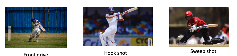
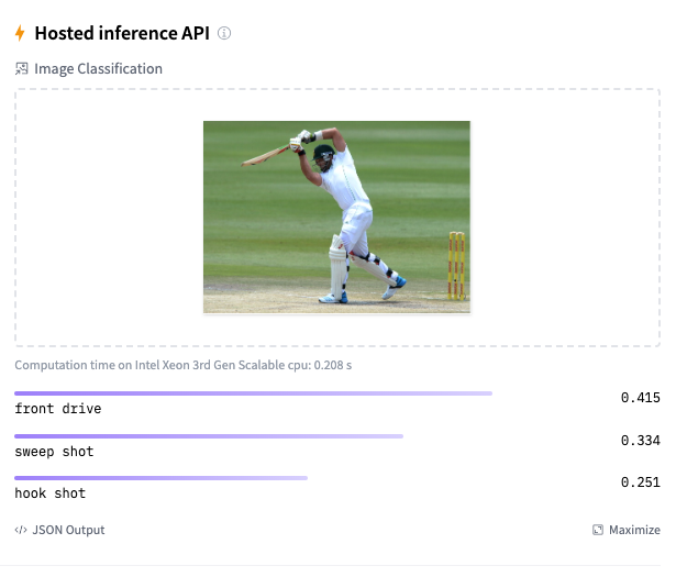
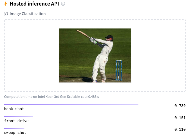


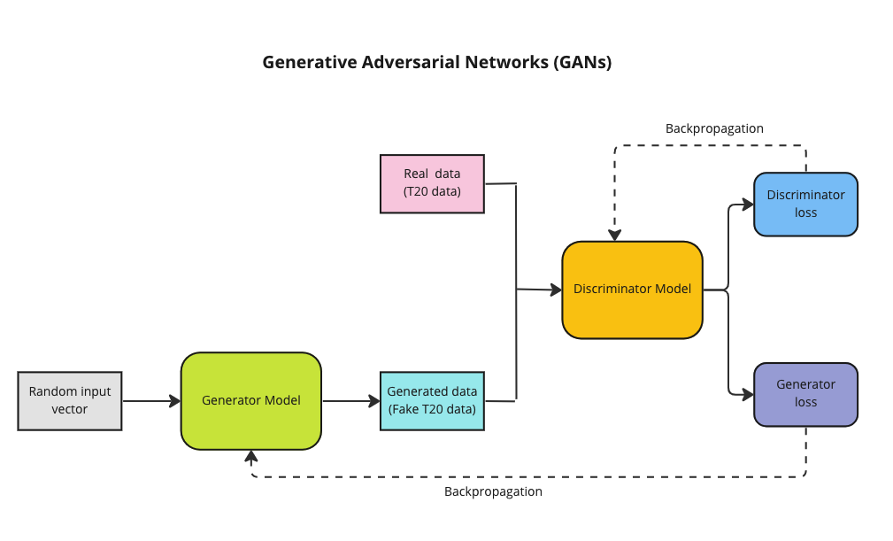
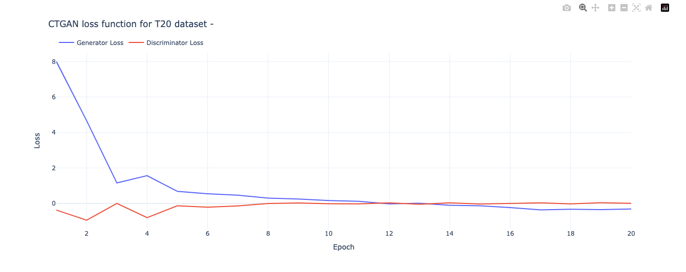
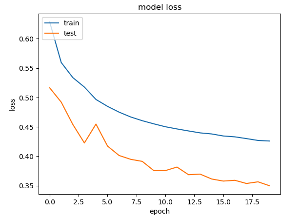

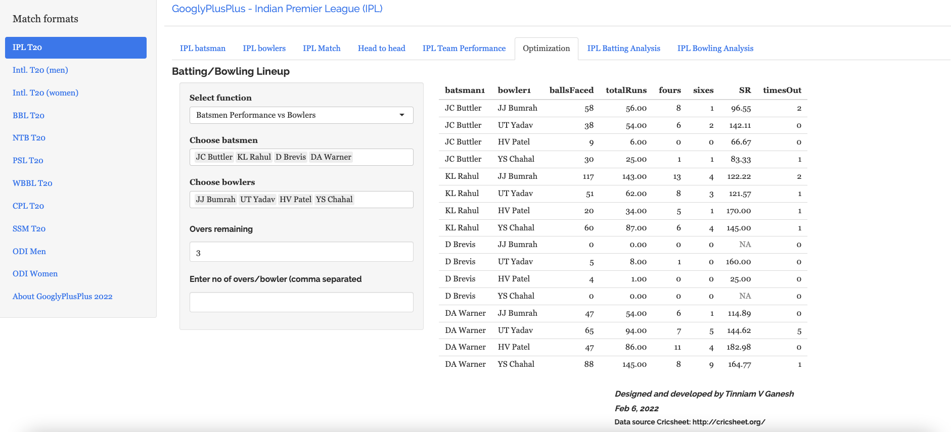
 ,
,  and
and  for the 3 bowlers which identify the characteristics of these bowlers (“fast”, “lateral drift through the air”, “movement off the pitch”). Let each batsman be identified by parameter vectors
  ,
,  and so on
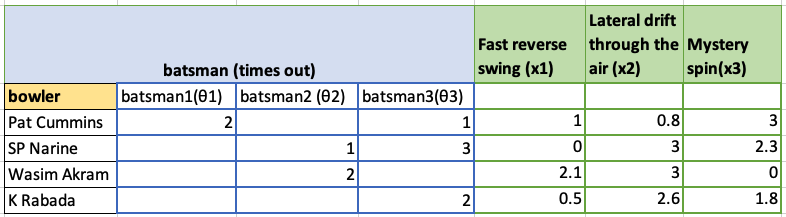
 and the feature vector xx we can formulate this as an optimization problem which tries to minimize the error for
  This can work very well as the algorithm can determine features which cannot be captured. So for e.g. some particular bowler may have very impressive figures. This could be due to some aspect of the bowling which cannot be captured by the data for e.g. let’s say the bowler uses the ‘scrambled seam’ when he is most effective, with a slightly different arc to the flight. Though the algorithm cannot identify the feature as we know it, but the ML algorithm should pick up intricacies which cannot be captured in data.
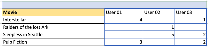
 ,
,  }= 1/2
 and the set of features be
  to small random values
 , i= 1,2,..,
 :=
:=  (
( 
 )
) –
– 
 :=
:= 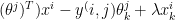

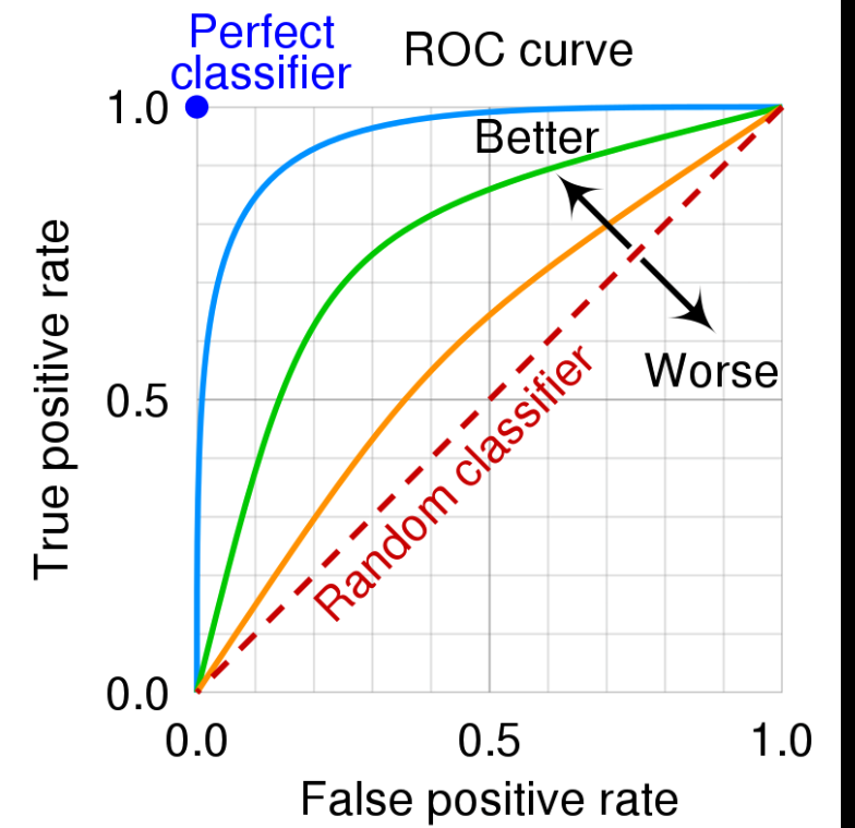
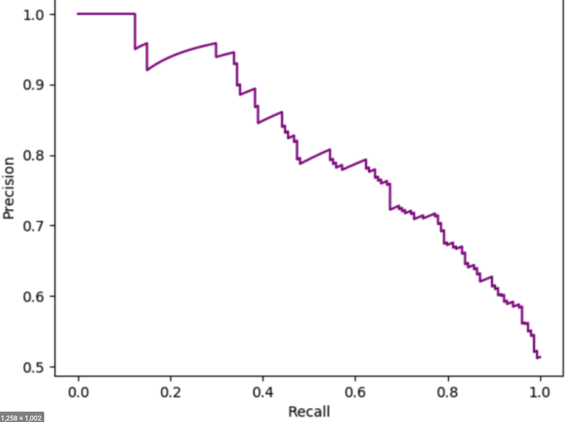
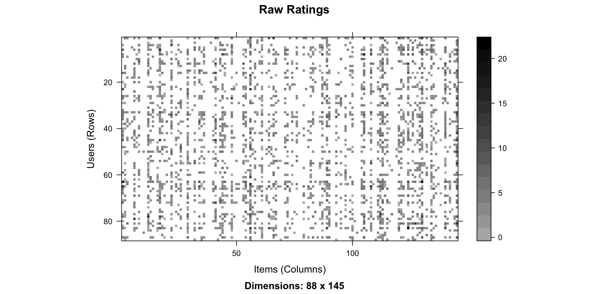
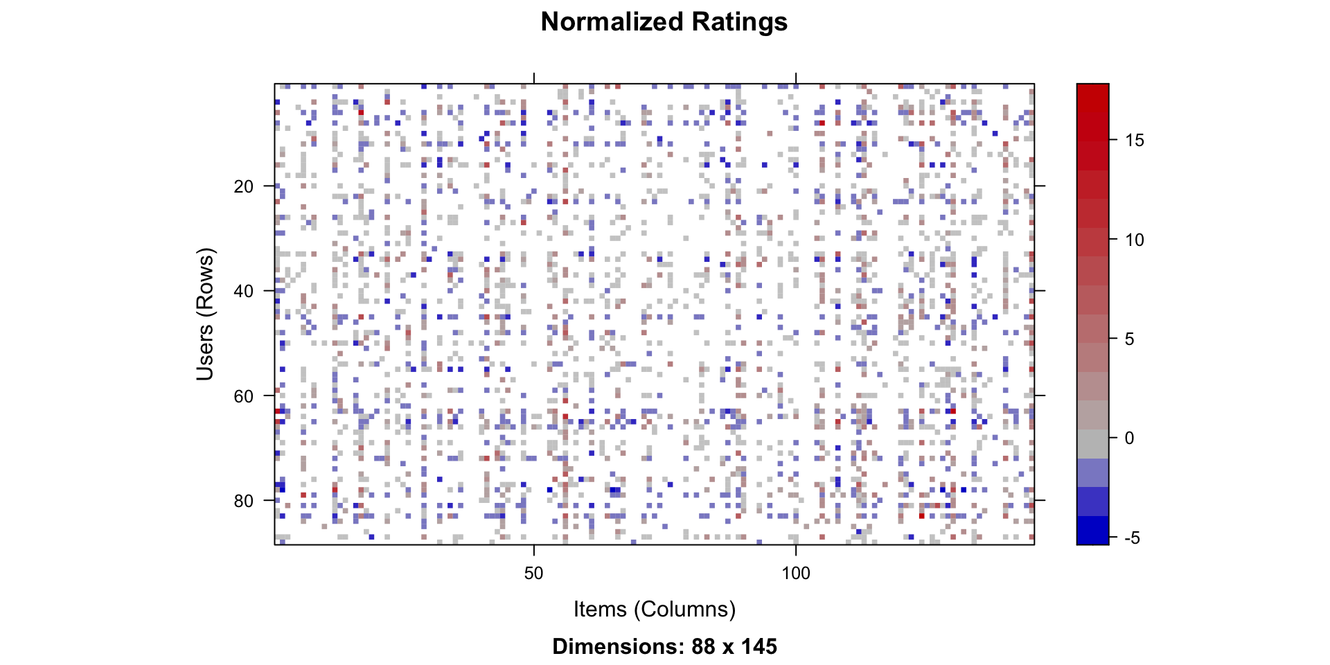
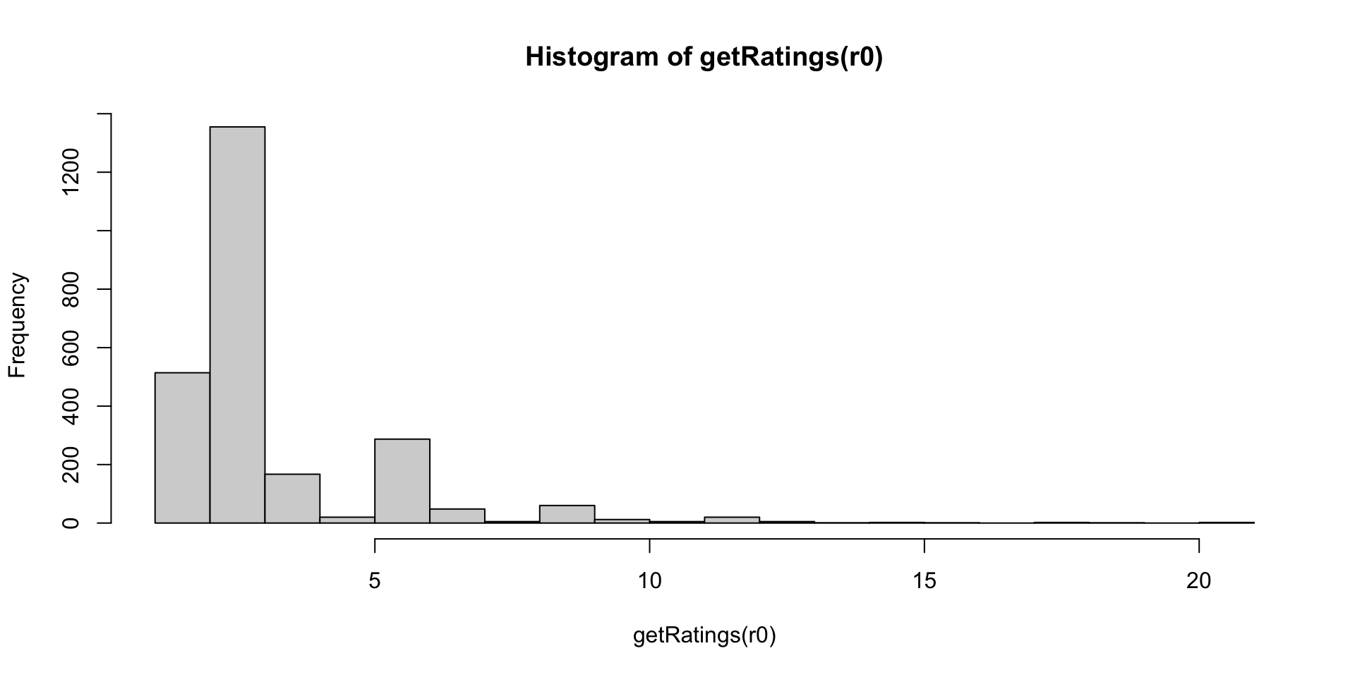
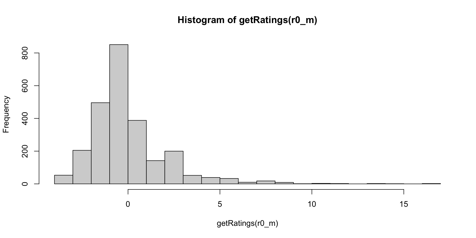
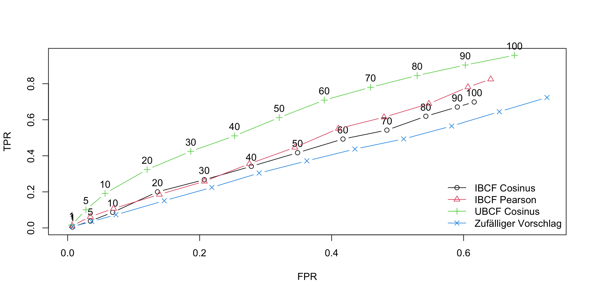


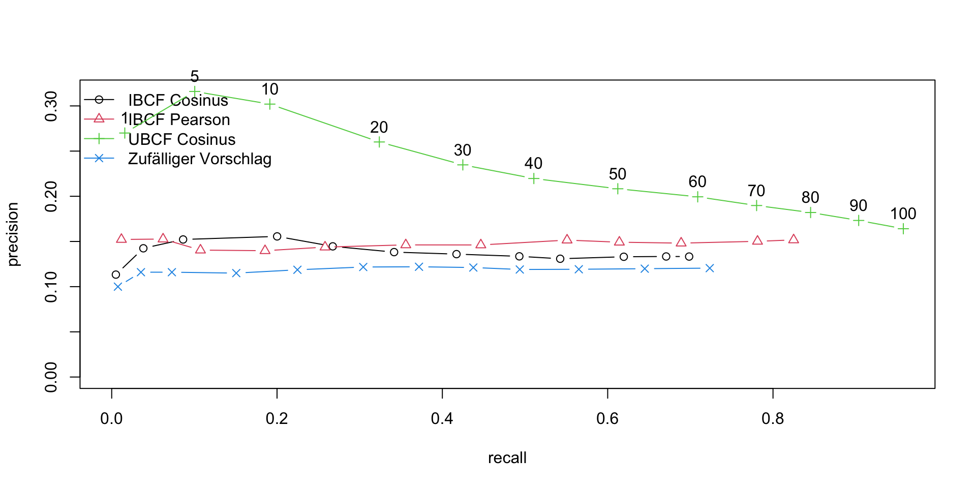
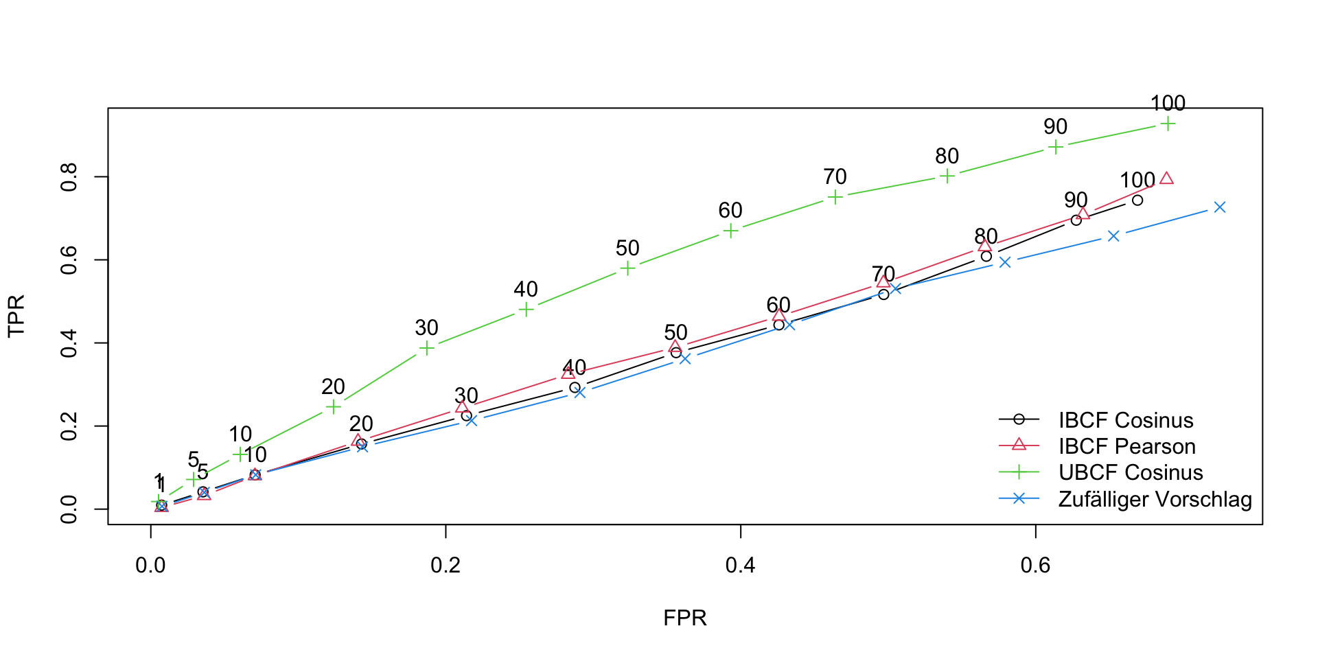
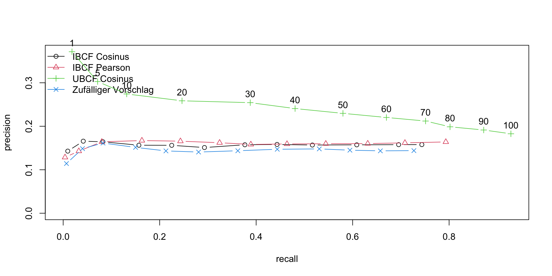
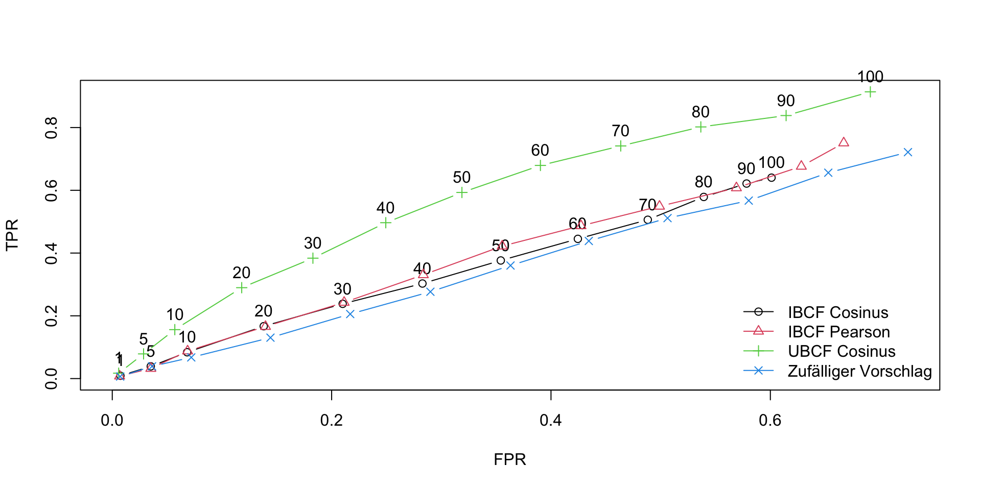
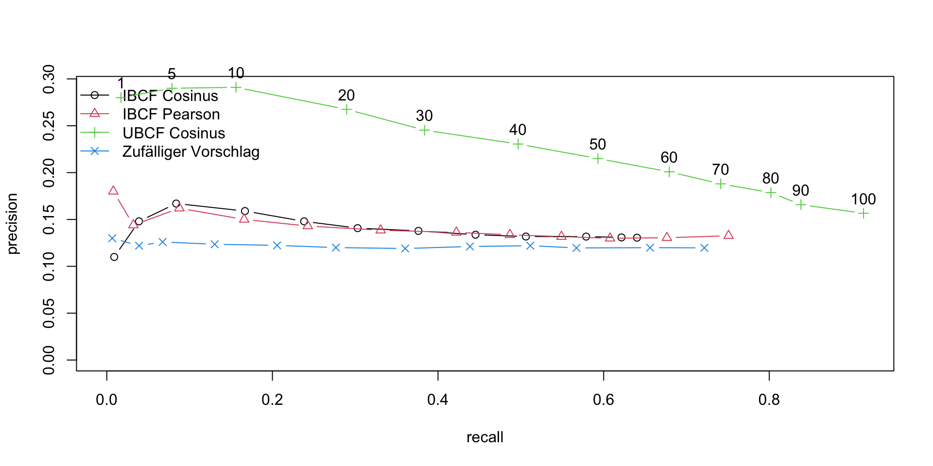
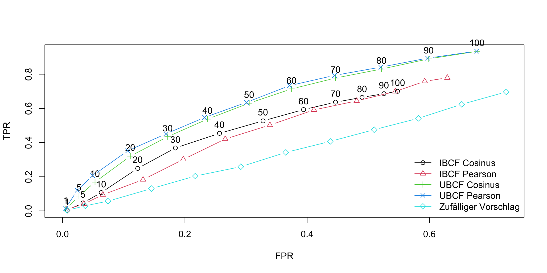
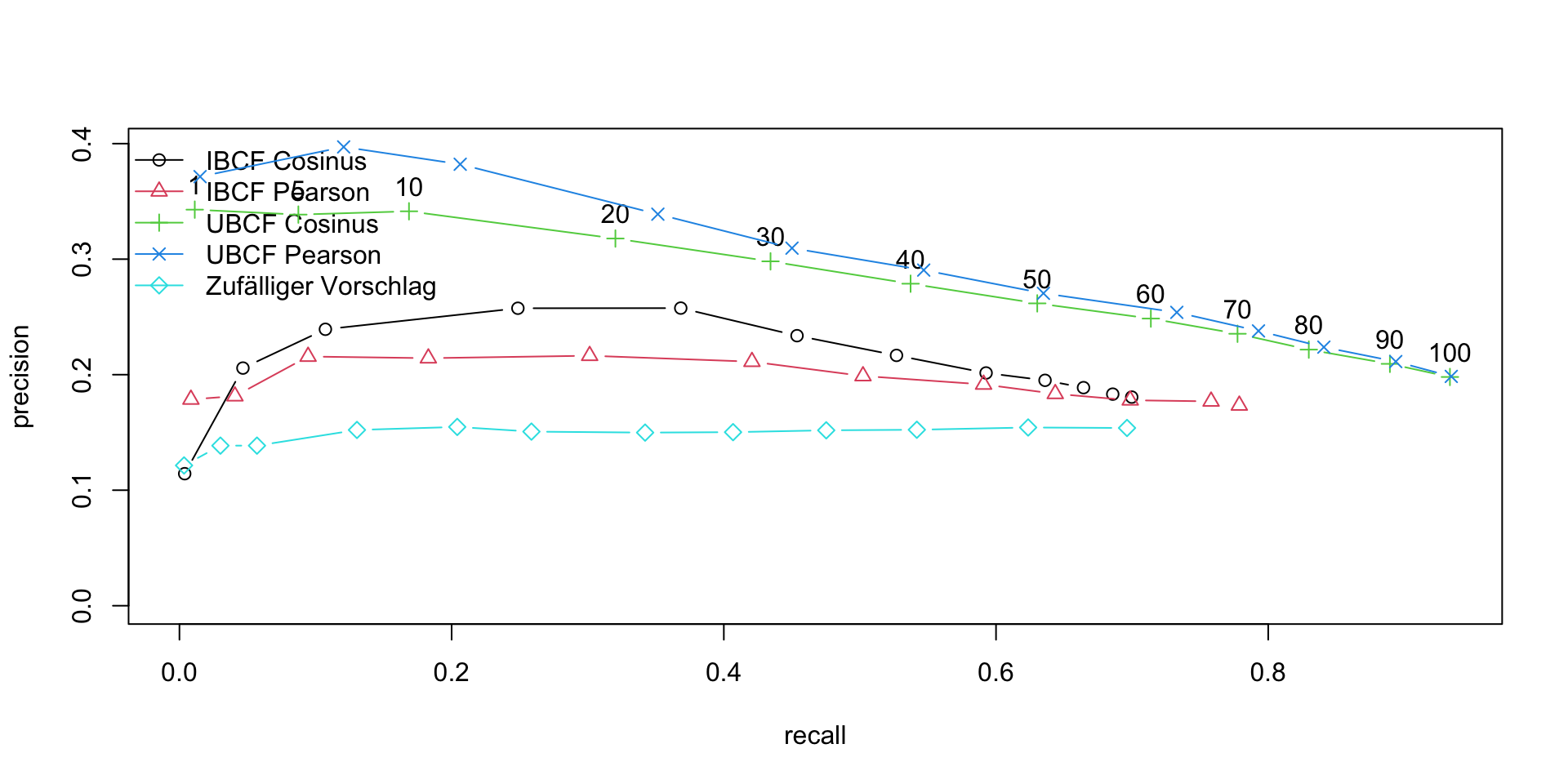
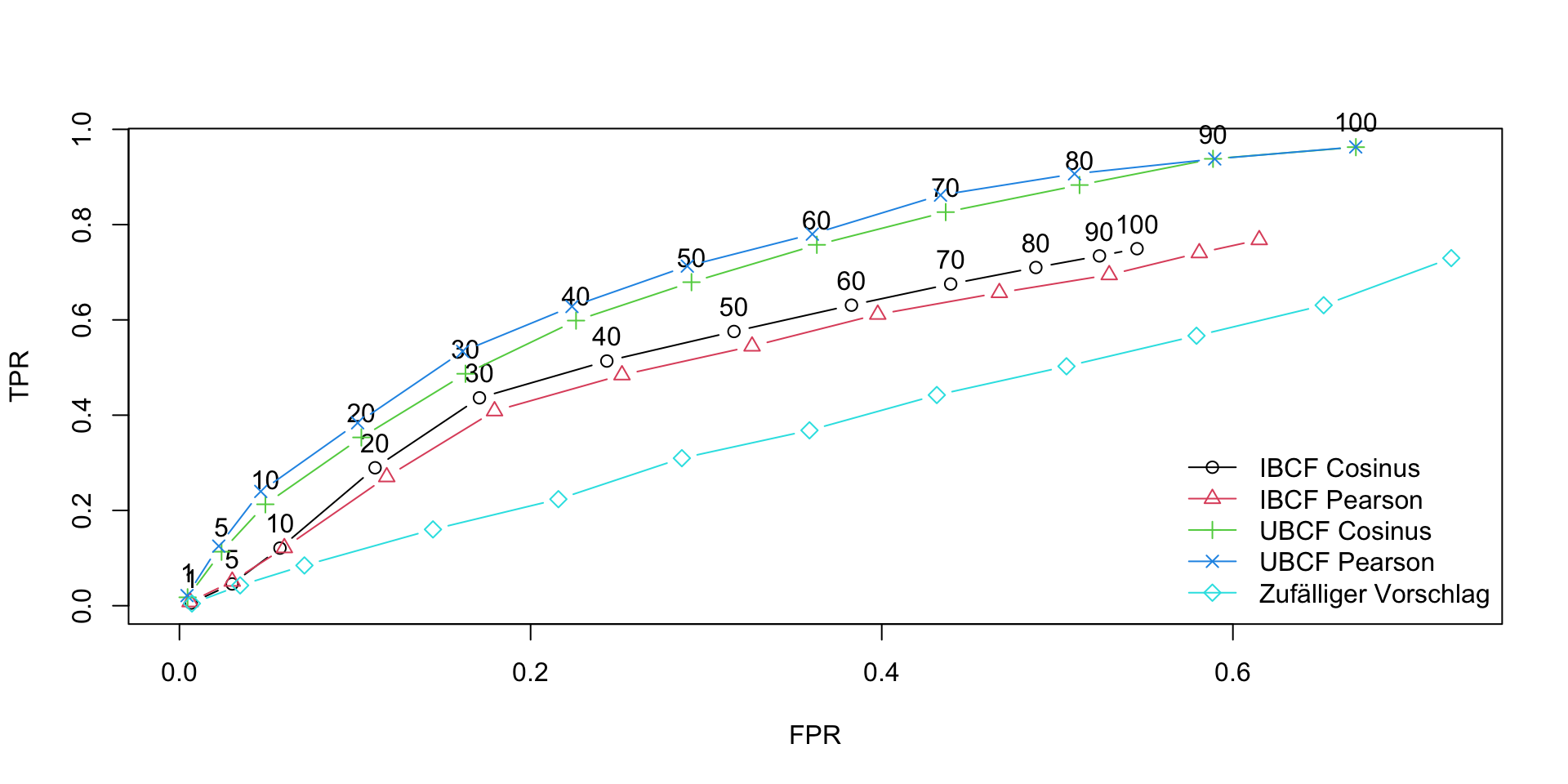
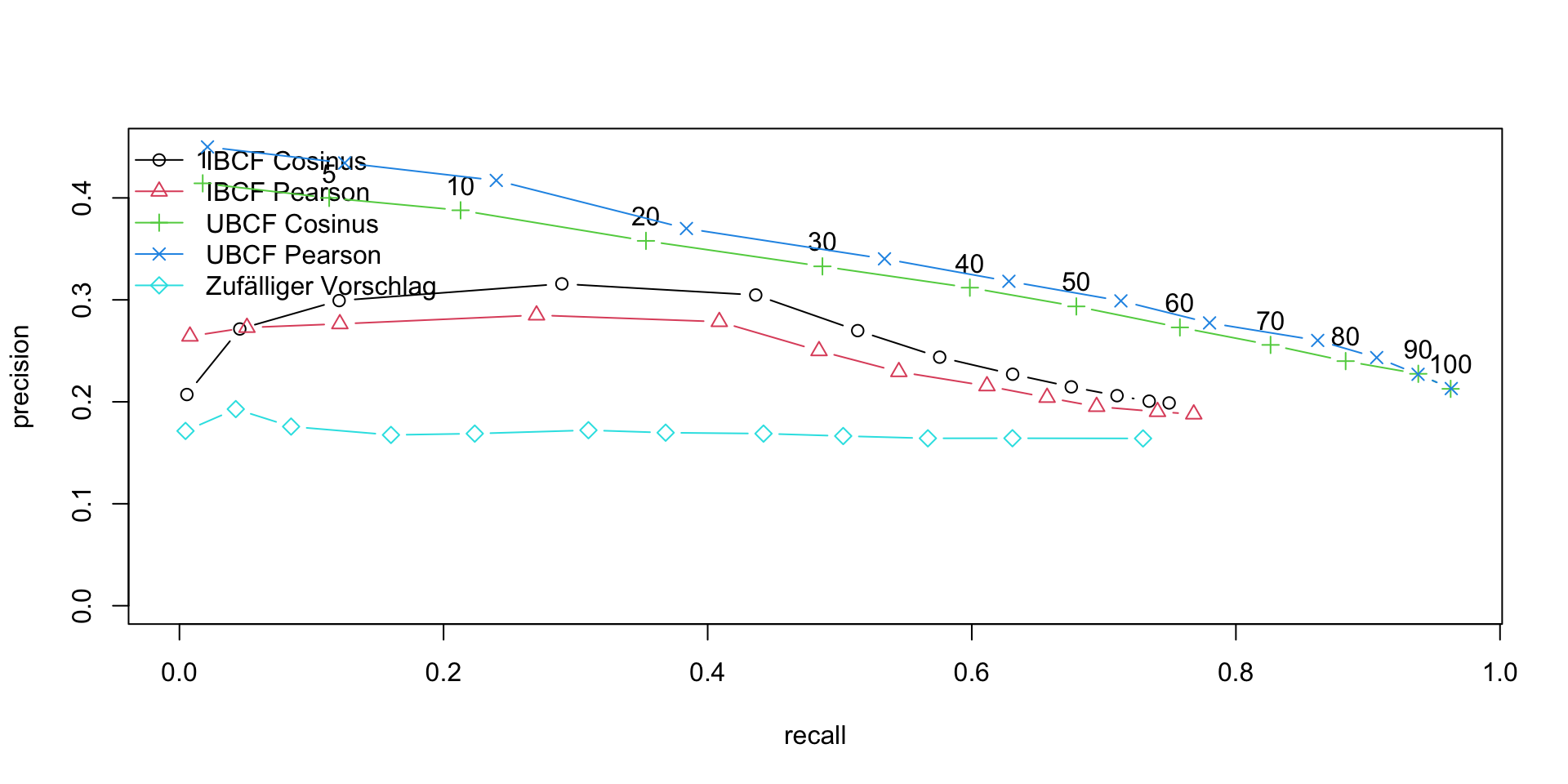
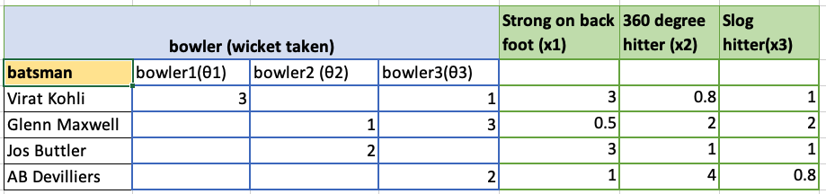
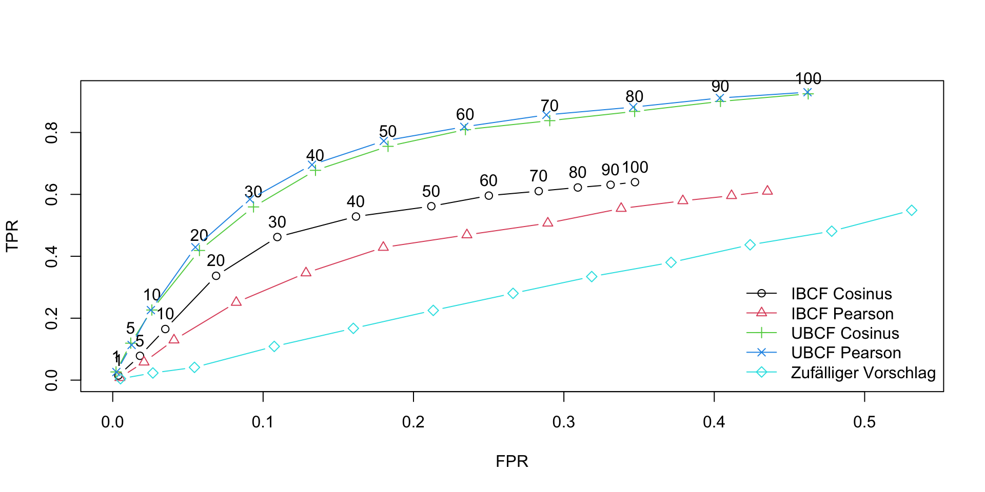
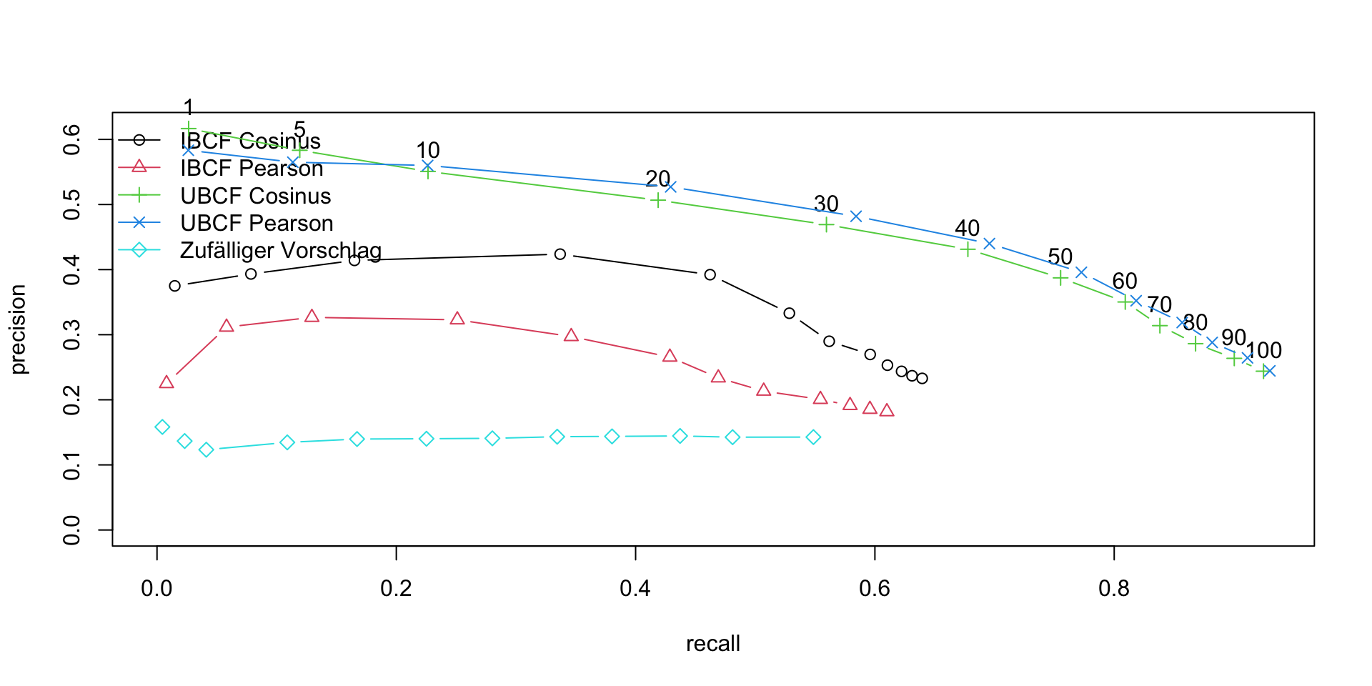
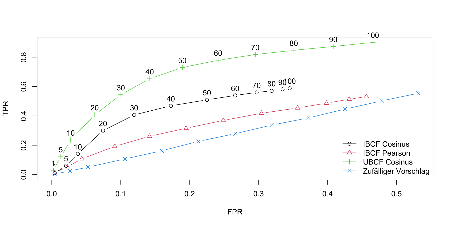
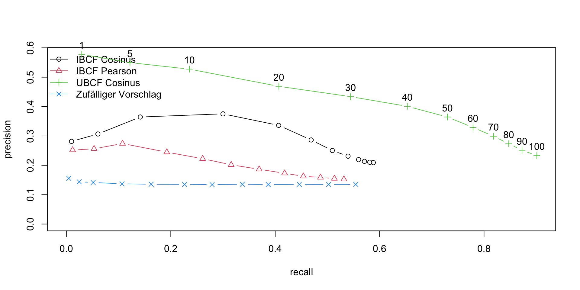
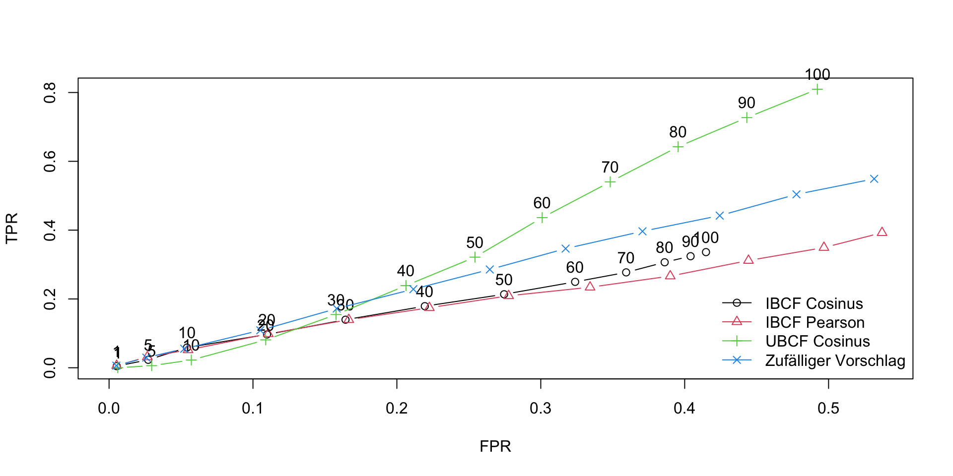
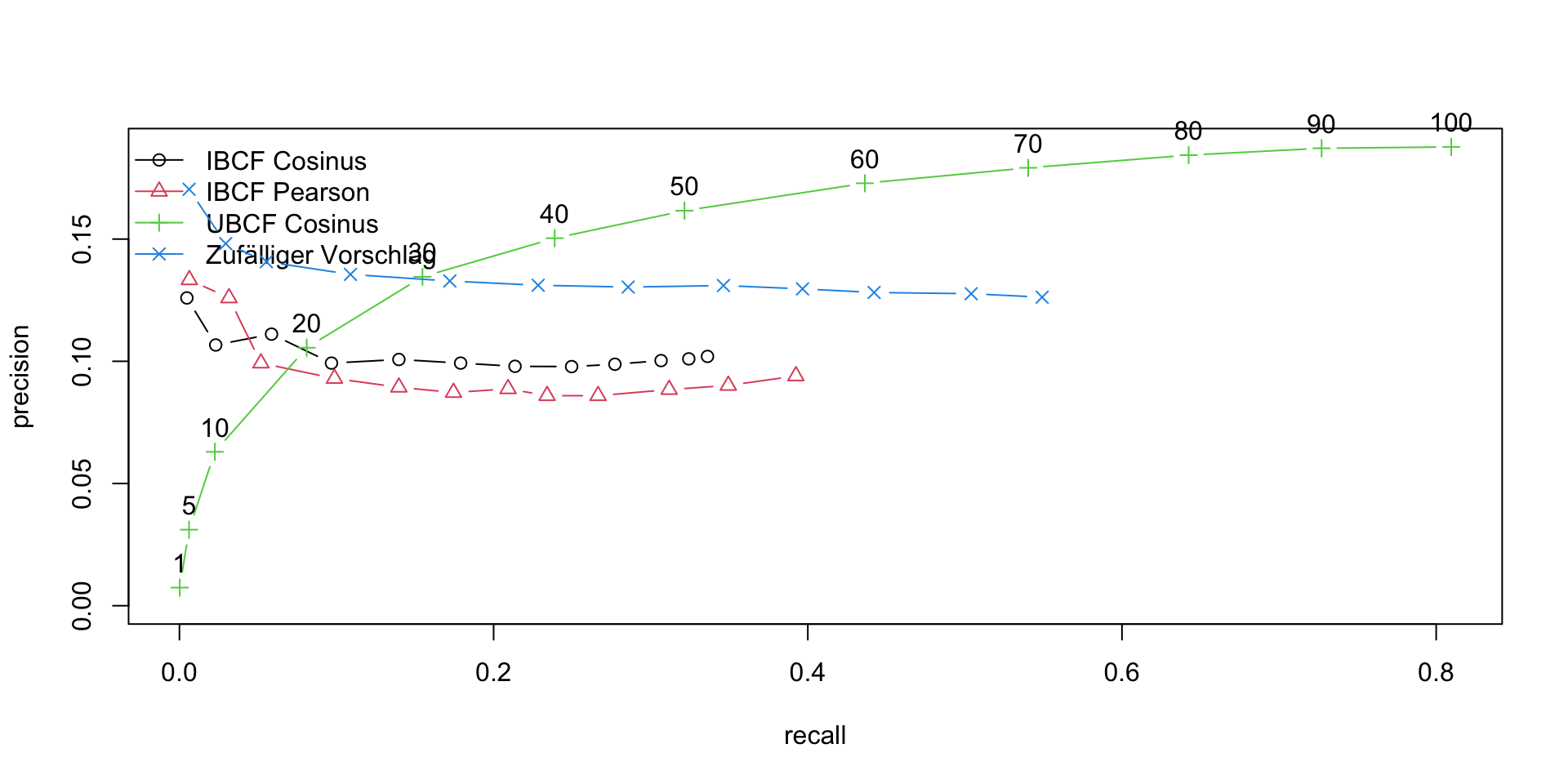
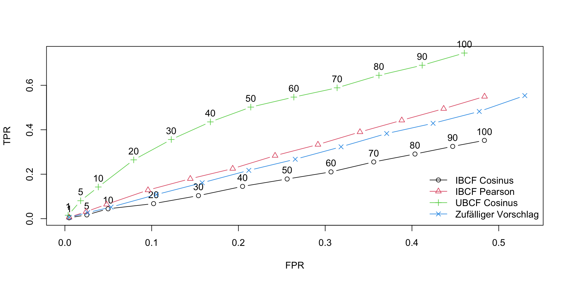
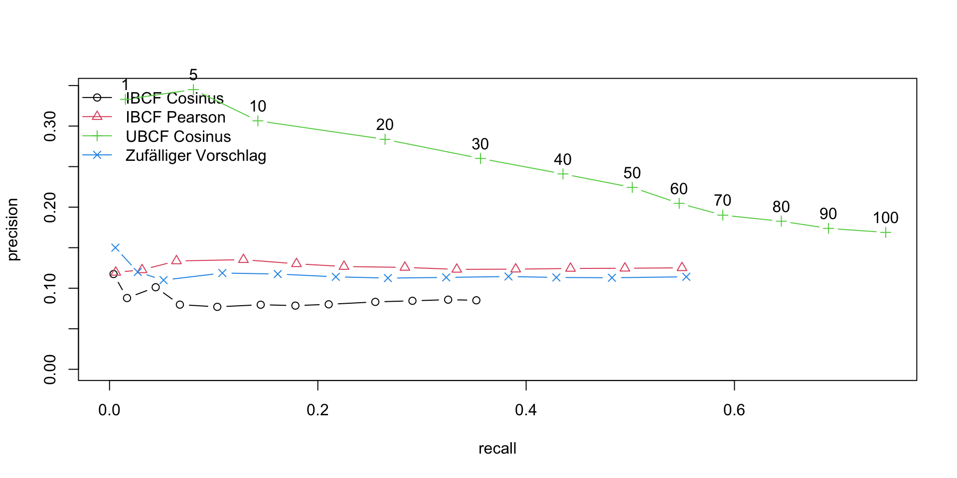


 and
and  represent the activations at layer ‘l’ in a filter i, at position ‘j’. The intuition is that the activations will be same for similar source and generated image. We need to minimise the content loss so that the generated stylized image is as close to the original image as possible. An intermediate layer of VGG19 block5_conv2 is used
 x
x 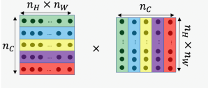
 and width
  with
with  channels
 and
and  are the Gram matrices of the style and generated images respectively. By minimising the distance in the gram matrices of the style and generated image we can ensure that generated image is a stylized version of the original image similar to the style image
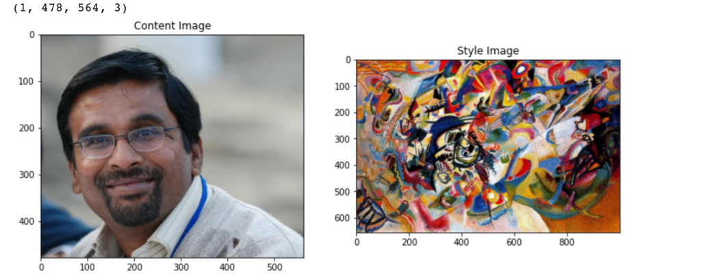


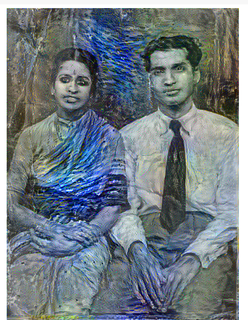
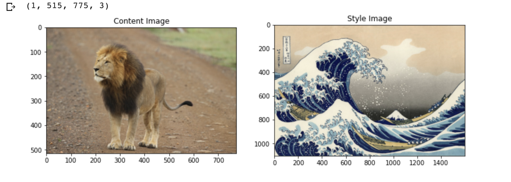
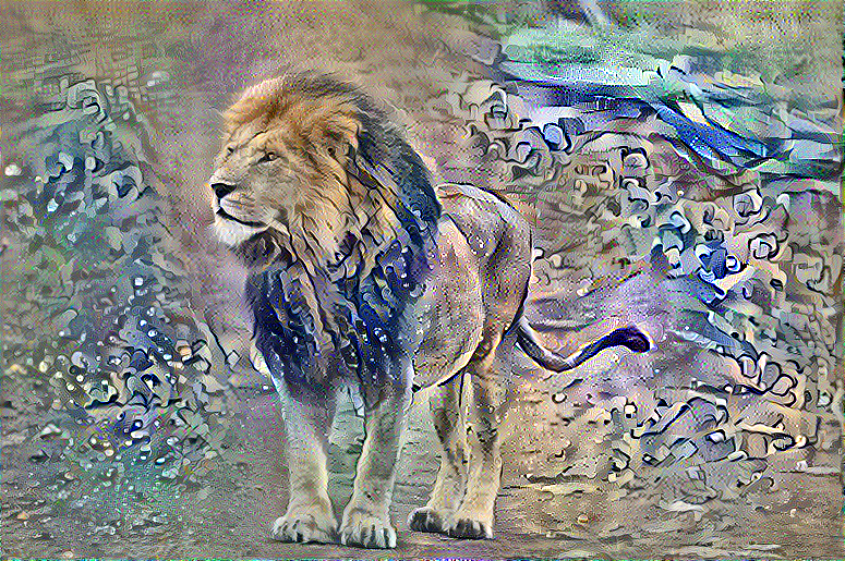
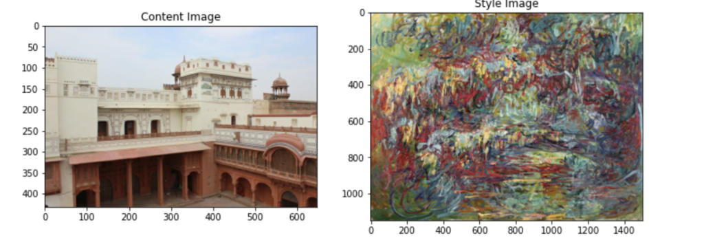
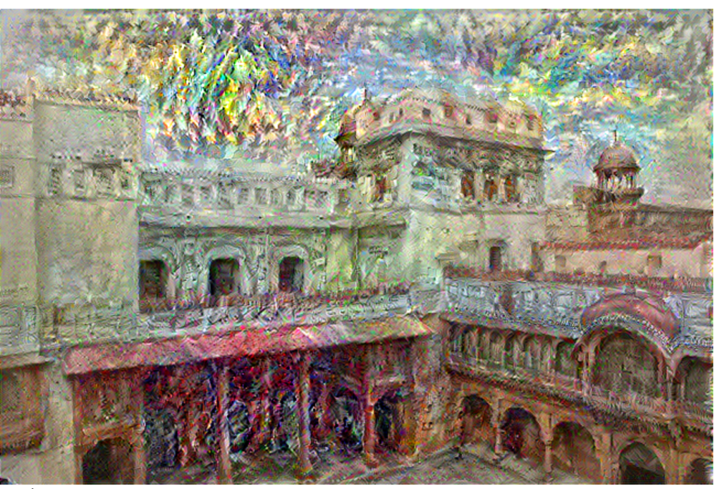

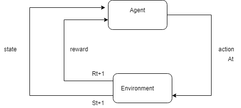
 where
where  is the expected return in time t and the discounted expected return
  in time t+1
 at time t, then
  is the probability that
  = a if
  = s.
= s. , is the expected return when starting in s and following
 ![v_{\pi}(s) = E_{\pi}[G_{t} |S_{t}=s] = E_{\pi}[\sum_{k=0}^{k=Inf} \gamma^{k}R_{t+k+1}|S_{t}=s]](https://s0.wp.com/latex.php?latex=v_%7B%5Cpi%7D%28s%29+%3D+E_%7B%5Cpi%7D%5BG_%7Bt%7D+%7CS_%7Bt%7D%3Ds%5D+%3D+E_%7B%5Cpi%7D%5B%5Csum_%7Bk%3D0%7D%5E%7Bk%3DInf%7D+%5Cgamma%5E%7Bk%7DR_%7Bt%2Bk%2B1%7D%7CS_%7Bt%7D%3Ds%5D&bg=ffffff&fg=000000&s=0&c=20201002)
![E_{\pi}[R_{t+1} + \gamma G_{t+1} |S_{t}=s]](https://s0.wp.com/latex.php?latex=E_%7B%5Cpi%7D%5BR_%7Bt%2B1%7D+%2B+%5Cgamma+G_%7Bt%2B1%7D+%7CS_%7Bt%7D%3Ds%5D&bg=ffffff&fg=000000&s=0&c=20201002)
![v_{\pi}(s)=\sum_{a} \pi(a|s) \sum_{s',r} p(s',r|s,a)[r+\gamma*v_{\pi}(s')]](https://s0.wp.com/latex.php?latex=v_%7B%5Cpi%7D%28s%29%3D%5Csum_%7Ba%7D+%5Cpi%28a%7Cs%29+%5Csum_%7Bs%27%2Cr%7D+p%28s%27%2Cr%7Cs%2Ca%29%5Br%2B%5Cgamma%2Av_%7B%5Cpi%7D%28s%27%29%5D&bg=ffffff&fg=000000&s=0&c=20201002)
![q_{\pi}(s,a)= \sum_{s',r} p(s',r|s,a)[r+\gamma*\pi(a|s)q_{\pi}(s',a')]](https://s0.wp.com/latex.php?latex=q_%7B%5Cpi%7D%28s%2Ca%29%3D+%5Csum_%7Bs%27%2Cr%7D+p%28s%27%2Cr%7Cs%2Ca%29%5Br%2B%5Cgamma%2A%5Cpi%28a%7Cs%29q_%7B%5Cpi%7D%28s%27%2Ca%27%29%5D&bg=ffffff&fg=000000&s=0&c=20201002)
![v_{*}(s)=max_{a}\sum_{s',r} p(s',r|s,a)[r+\gamma*v_{*}(s')]](https://s0.wp.com/latex.php?latex=v_%7B%2A%7D%28s%29%3Dmax_%7Ba%7D%5Csum_%7Bs%27%2Cr%7D+p%28s%27%2Cr%7Cs%2Ca%29%5Br%2B%5Cgamma%2Av_%7B%2A%7D%28s%27%29%5D&bg=ffffff&fg=000000&s=0&c=20201002)
![q_{*}(s,a)=\sum_{s',r} p(s',r|s,a)[r+\gamma*max_{a}q_{*}(s',a')]](https://s0.wp.com/latex.php?latex=q_%7B%2A%7D%28s%2Ca%29%3D%5Csum_%7Bs%27%2Cr%7D+p%28s%27%2Cr%7Cs%2Ca%29%5Br%2B%5Cgamma%2Amax_%7Ba%7Dq_%7B%2A%7D%28s%27%2Ca%27%29%5D&bg=ffffff&fg=000000&s=0&c=20201002)
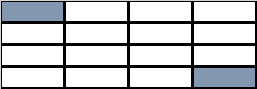
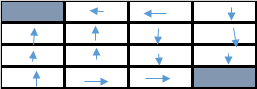

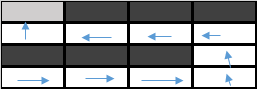
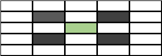
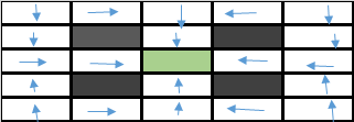

 Checkout my book ‘Deep Learning from first principles: Second Edition – In vectorized Python, R and Octave’. My book starts with the implementation of a simple 2-layer Neural Network and works its way to a generic L-Layer Deep Learning Network, with all the bells and whistles. The derivations have been discussed in detail. The code has been extensively commented and included in its entirety in the Appendix sections. My book is available on Amazon as
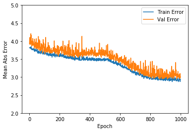


 Checkout my book ‘Deep Learning from first principles: Second Edition – In vectorized Python, R and Octave’. My book starts with the implementation of a simple 2-layer Neural Network and works its way to a generic L-Layer Deep Learning Network, with all the bells and whistles. The derivations have been discussed in detail. The code has been extensively commented and included in its entirety in the Appendix sections. My book is available on Amazon as
 Checkout my book ‘Deep Learning from first principles: Second Edition – In vectorized Python, R and Octave’. My book starts with the implementation of a simple 2-layer Neural Network and works its way to a generic L-Layer Deep Learning Network, with all the bells and whistles. The derivations have been discussed in detail. The code has been extensively commented and included in its entirety in the Appendix sections. My book is available on Amazon as


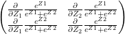 – (A)
– (A)


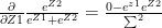
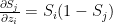 when i=j
 when
when 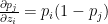 when i=j

 when i=j and 0 when


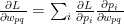 (1)
(1) (2)
(2)
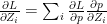


 when i=j
 when
when 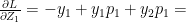


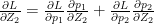

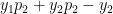
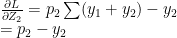


 which similarly reduces to


 and
and 
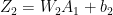 and
and 


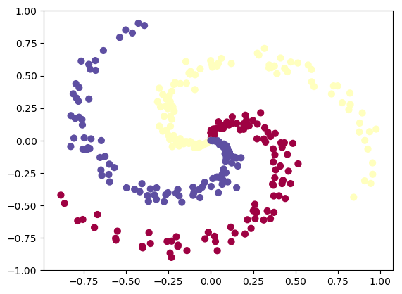

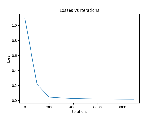
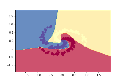

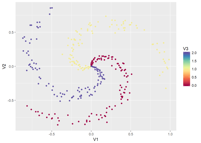
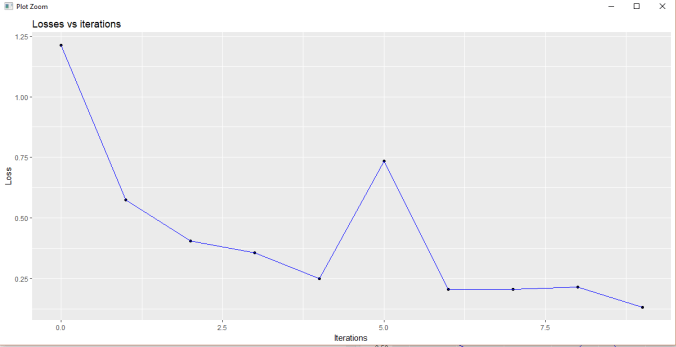
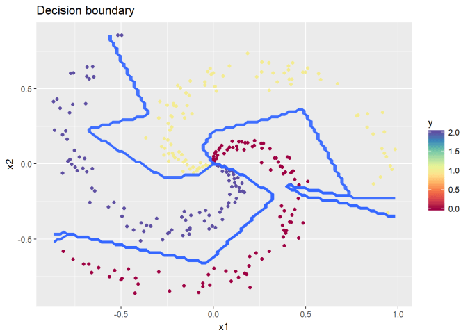
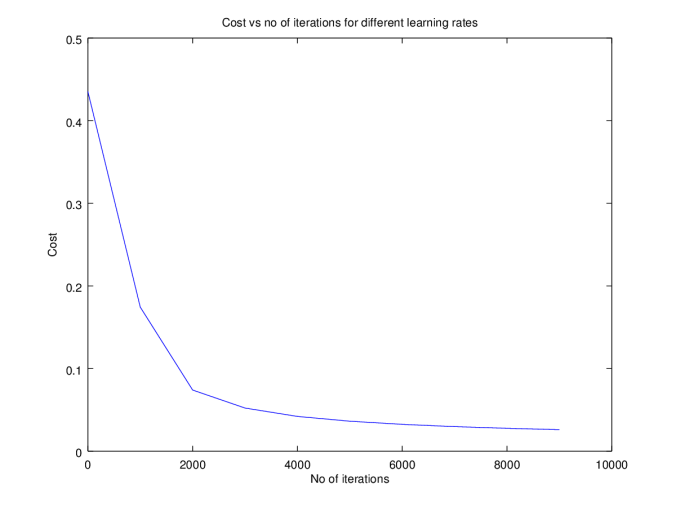
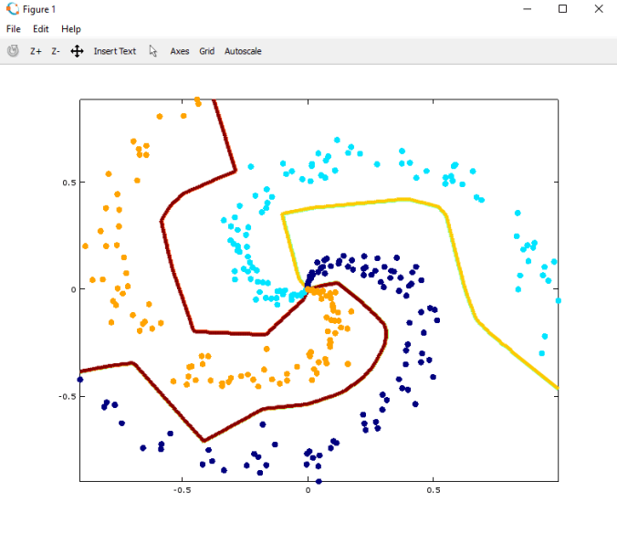


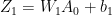 and
and 
 and
and 


 . It can be shown that
 see equation 2 in
  see equation (f) in
  because
  -(1a)
-(1a) -(1b)
-(1b) -(1c)
-(1c)
 -(1d)
-(1d)
 – (2a)
 – (2b)
 – (2c)
 – (2d)
 and
and 


 = a g’(z) = a(1-a) – See
 , …
, … ![v_{L-1}]](https://s0.wp.com/latex.php?latex=v_%7BL-1%7D%5D&bg=ffffff&fg=000000&s=0&c=20201002)
 , …
, … 
 …
… ![v_{L}]](https://s0.wp.com/latex.php?latex=v_%7BL%7D%5D&bg=ffffff&fg=000000&s=0&c=20201002)
 is the number of activation units in each hidden layer, which is specified while actually executing the Deep Learning network using the function L_Layer_DeepModel(), in all the implementations Python, R and Octave
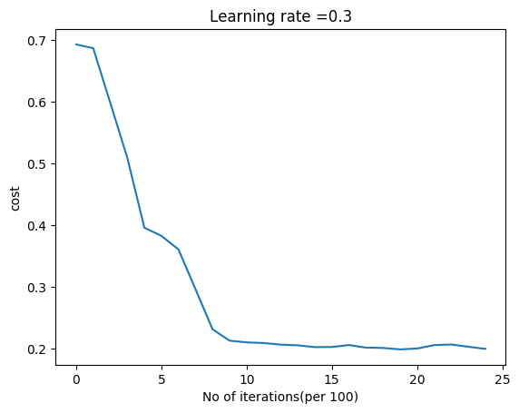
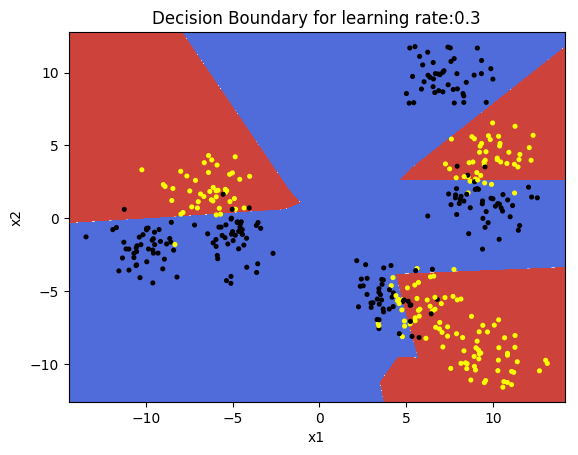

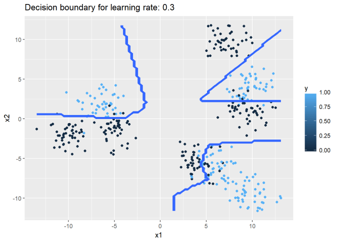
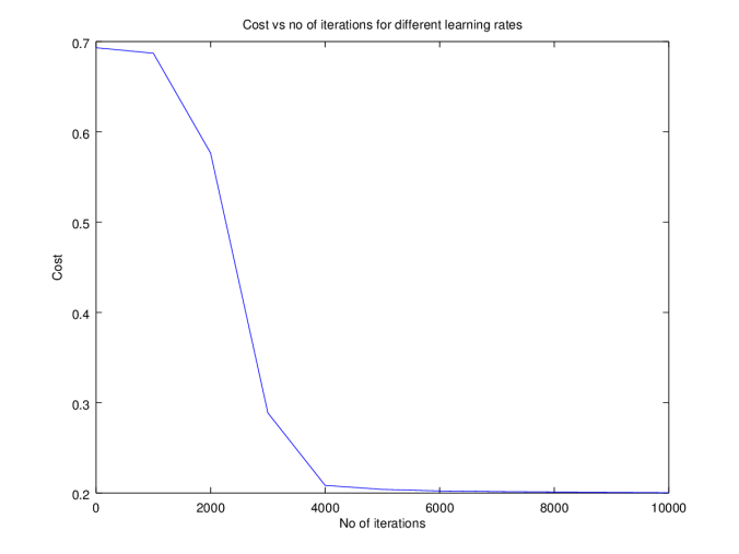

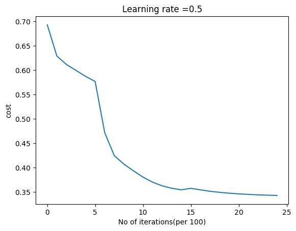
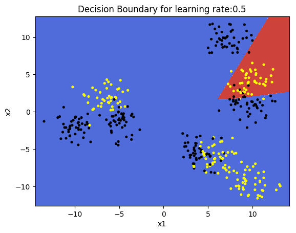

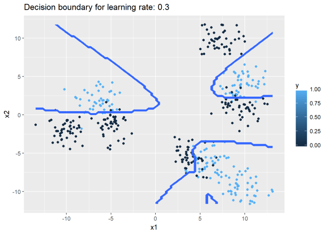
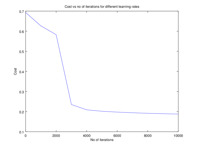
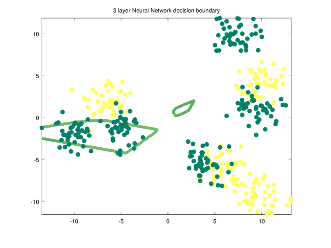
 =
=